Features of the Flow Structure in the Vicinity of the Inner Lagrangian Point in Polars

Abstract

The structures of plasma flows in close binary systems whose accretors have strong intrinsic magnetic fields are studied. A close binary system with the parameters of a typical polar is considered. The results of three dimensional numerical simulations of the material flow from the donor into the accretor Roche lobe are presented. Special attention is given to the flow structure in the vicinity of the inner Lagrangian point, where the accretion flow is formed. The interaction of the accretion flow material from the envelope of the donor with the magnetic field of the accretor results in the formation of a hierarchical structure of the magnetosphere, because less dense areas of the accretion flow are captured by the magnetic field of the white dwarf earlier than more dense regions. Taking into account this kind of magnetosphere structure can affect analysis results and interpretation of the observations.

1 Introduction

Cataclysmic variables consist of a donor star (a low mass, late type star) and an accretor star (a white dwarf) [1]. The donor’s envelope fills its Roche lobe. At the inner Lagrangian point, the pressure gradient is not balanced by the gravity. As a result, material starts to flow into the Roche lobe of the compact object. There is a wide class of cataclysmic variable in which the magnetic field can substantially influence the mass exchange and accretion processes. Magnetic cataclysmic variables can be divided into polars and intermediate polars. In intermediate polars, the magnetic field of the accretor is relatively weak ($10-1000~{}\text{kG}$), and an accretion disk can be formed in the system [2]. In polars, the magnetic field of the accretor is strong ($>1~{}\text{MG}$), and prevents the formation of the accretion disk. The material streaming from the donor forms a collimated stream that moves along the magnetic field lines and reaches one of the magnetic poles of the accretor.

The magnetic fields in a close binary system does not only influence the motion of the stream from the donor envelope, but also controls the formation of this stream [3, 4, 5]. This situation can arise in polars with strong magnetic fields (about $100~{}\text{MG}$ and higher), when the donor envelope is located partially in the magnetosphere of the white dwarf. The results of 3D numerical simulations of the flow structure in such systems [2] show that the material streaming from the donor immediately splits into several flows, which move along magnetic field lines and reach the magnetic poles of the accretor. This flow pattern does not correspond to the classical picture of the formation of a stream from the donor to the Roche lobe of the accretor through the inner Lagrangian point [6]. Taking into account the effect of the common envelope of a binary system can considerably change the flow pattern in the vicinity of the inner Lagrangian point [7]. However, this effect is apparently more strongly manifest in intermediate polars, since almost all the material from the donor envelope falls on the accretor in polars.

In earlier studies, we have developed a 3D numerical model that can be used to study accretion in semidetached binary systems taking into account the magnetic field of the accretor [8]. In our previous simulations, the material flow from the inner Lagrangian point towards the Roche lobe of the accretor was determined by the boundary conditions. This model enables us to study only the influence of a magnetic field on the already formed accretion stream. In the numerical model presented in our current study, the material flow from the donor is defined by a natural way, rather than by the imposed boundary conditions. Therefore, this model can be used to study the influence of the magnetic field on the formation of the accretion flow.

The paper is organized as follows. In Section 2, we analyze the parameters that can affect the flow structure, such as the radius of the white dwarf magnetosphere. In Section 3, we discuss the formulation of the problem and describe our numerical model. The results of the numerical simulations are presented in Section 4. We discuss our main results in the Conclusion.

2 Estimates of the Radius of the Accretor Magnetosphere

A simple way to estimate the radius of the accretor magnetosphere in polar type systems is to take it to be comparable to the corresponding Alfvèn radius $R_{\text{m}}$ [13]. Let us consider the material stream moving from the vicinity of the Lagrangian point towards the accretor. This stream is stopped by the magnetic field at some distance from the accretor. We can estimate this distance by writing the condition for equality of the magnetic and dynamical pressures:

$${\displaystyle\frac{B_{*}^{2}}{8\pi}}=\rho v^{2},$$ (1)

where $v=\sqrt{2GM_{\text{a}}/r}$ is the free-fall velocity, $G$ the gravitational constant, and $M_{\text{a}}$ the mass of the accretor. The density $\rho$ can be calculated from the mass transfer rate: $\dot{M}=S\rho v$, where $S$ is the cross section of the accretion stream. Generally, the magnetic field of the accretor in a typical polar can be described by a dipole field [14]:

$${{\bm{B}}}_{*}=\frac{\mu}{r^{3}}\left[3({\bm{d}}\cdot{\bm{n}}){\bm{n}}-{\bm{d}}\right],$$ (2)

where $\mu=B_{\text{a}}R_{\text{a}}^{3}/2$ is the magnetic moment, $B_{\text{a}}$ the magnetic field at the surface of the white dwarf, $R_{\text{a}}$ the radius of the white dwarf, and ${{\bm{d}}}$ a unit vector determined by the axis of symmetry of the dipole field. The vector magnetic moment is ${{\bm{\mu}}}=\mu{{\bm{d}}}$ and the unit vector is ${{\bm{n}}}={{\bm{r}}}/r$. Let us assume that the accretor’s center is located at the coordinate origin. The components of the magnetic moment ${\bm{\mu}}$ are

$$\mu_{x}=\mu\sin\theta\cos\phi,\quad\mu_{y}=\mu\sin\theta\sin\phi,\quad\mu_{z}=\mu\cos\theta,$$ (3)

where $\theta$ is the inclination of the vector ${\bm{\mu}}$ relative to the $z$, and $\phi$ is the angle between the projection of ${\bm{\mu}}$ onto the equatorial plane of the binary system ($xy$) and the $x$ axis. In our model, we assumed that the rotation and orbital motion of the components is synchronous, so that the phase angle $\phi$ is time independent. The magnetic field ${\bm{B}}_{*}$ is potential in the computational domain, $\nabla\times{\bm{B}}_{*}=0$, This enables us to partially exclude this field from the equations describing the structure of the magnetohydrodynamical (MHD) flows [8, 9, 10].

The cross sectional area of the stream of material from the donor in the vicinity of the inner Lagrangian point can be estimated by the expression [6, 8]:

$$S={\displaystyle\frac{\pi c_{\text{s}}^{2}}{4\Omega^{2}}}g_{y}\left(q\right)g_{z}\left(q\right),$$ (4)

where $g_{y}\left(q\right)$ and $g_{z}\left(q\right)$ are functions that depend on the component mass ratio $q=M_{\text{d}}/M_{\text{a}}$ ($M_{\text{d}}$ is the mass of the donor) that are close to the unity and determine the size of the stream along the $y$ and $z$, axis, while $\Omega$ is the orbital angular velocity of the system. Using these relations and Eq. (1), we can obtain the estimate

$$R_{\text{m}}=\left[{\displaystyle\frac{B_{\text{a}}^{4}R_{\text{a}}^{12}S^{2}}{128\pi^{2}GM_{\text{a}}\dot{M}^{2}}}\right]^{1/11}.$$ (5)

We estimated the magnetosphere radius using the parameters of a typical polar, taking as an example the orbital parameters of SS Cyg [11]. The donor (red dwarf) has the mass $M_{\text{d}}=0.56~{}M_{\odot}$ and the effective temperature $T_{\text{eff, d}}=4\,000~{}\text{K}$. The mass of the accretor is $M_{\text{a}}=0.97~{}M_{\odot}$, its radius is $R_{\text{a}}=7.3\cdot 10^{-3}~{}R_{\odot}$, and its effective temperature is $T_{\text{eff, a}}=37\,000~{}\text{K}$. The binary orbital period is $P_{\text{orb}}=2.4\cdot 10^{4}~{}\text{s}$. The distance between the binary components is $A=2.05~{}R_{\odot}$, and the inner Lagrangian point is placed at a distance $r_{\text{L}_{1}}=0.556~{}A$ from the accretor. The sound speed at the point L₁ is defined to be $c_{\text{s}}=7.4\cdot 10^{5}~{}\text{ cm/s}$, and the mass transfer rate through the vicinity of the inner Lagrangian point is $\dot{M}=10^{-10}~{}M_{\odot}/~{}\text{yr}$. Let us consider the case of a strong magnetic field, when the field at the surface of the white dwarf is $B_{\text{a}}=10^{8}~{}\text{G}$.

These values give a cross section for the stream at the inner Lagrangian point of $S=0.000332~{}A^{2}$. The corresponding diameter of the stream cross section is 2 $2\sqrt{S/\pi}=0.0206~{}A$. The magnetosphere radius is $R_{\text{m}}=0.14~{}A$.

The material in the stream is stopped at the magnetosphere radius by the magnetic field. However, it is clear that the magnetic field begins to influence the flow dynamics much earlier. We can estimate the distance at which this influence begins using the expressions for the forces acting on the stream material in our model (see the next Section). There are two forces acting on the material in the Roche lobe of the accretor: the gravitational force of the white dwarf and the friction force from its magnetic field. Let us determine the distance $R_{\text{w}}$, at which these forces become equal:

$${\displaystyle\frac{GM_{\text{a}}}{r^{2}}}={\displaystyle\frac{v}{t_{w}}}.$$ (6)

Here, $t_{w}$ is the decay time scale for the transverse velocity, determined by the expression:

$$t_{w}={\displaystyle\frac{4\pi\rho}{B_{*}^{2}}}\eta_{w},$$ (7)

$\eta_{w}$ is the magnetic viscosity coefficient associated with MHD wave turbulence,

$$\eta_{w}=\alpha_{w}{\displaystyle\frac{l_{w}B_{*}}{\sqrt{4\pi\rho}}},$$ (8)

where $\alpha_{w}$ is a dimensionless coefficient, which we took to be $1/3$, corresponding to isotropic turbulence [12], and $l_{w}=B_{*}/|\nabla B_{*}|$ is the characteristic spatial scale of the wave pulsations. Given Eq. (2) we can set $l_{w}=r/3$. Using the resulting relation, we find from (6)

$$R_{\text{w}}=\left[{\displaystyle\frac{81B_{*}^{4}R_{\text{a}}^{12}S^{2}}{2\pi^{2}\alpha_{w}^{4}GM_{\text{a}}\dot{M}^{2}}}\right]^{1/11}.$$ (9)

Note that this expression differs from (5) only in the numerical coefficients. Substituting the parameter values gives $R_{\text{w}}=0.46~{}A$, which is about a factor of three larger than the Alfvèn radius (5). It is easy to show that the friction force $f=v/t_{w}$ due to the magnetic field of the accretor is the dominant force at the Alfvèn radius; its value relative to the gravitational force $g=GM_{\text{a}}/r^{2}$ is $f/g\left(R_{\text{m}}\right)=25.5$. This means that the plasma flows inside this zone are fully governed by the magnetic field of the white dwarf.

3 Formulation of the Problem

We described the plasma flow structure in a magnetic close binary system using a non-inertial reference frame rotating about its center of mass with the orbital angular velocity $\Omega=2\pi/P_{\text{orb}}$, where $P_{\text{orb}}$ is the orbital period. The force field acting on the material in this frame is determined by the Roche potential, which has the form

$$\Phi=-\frac{GM_{\text{a}}}{|{\bm{r}}-{\bm{r}}_{\text{a}}|}-\frac{GM_{\text{d}}}{|{\bm{r}}-{\bm{r}}_{\text{d}}|}-\frac{1}{2}\left[{\bm{\Omega}}\times\left({\bm{r}}-{\bm{r}}_{\text{c}}\right)\right]^{2},$$ (10)

where the radius vectors ${\bm{r}}_{\text{a}}$, ${\bm{r}}_{\text{d}}$, and ${\bm{r}}_{\text{c}}$ define the accretor’s center, the donor’s center, and the center of mass of the binary system, respectively. The first and second terms in (10) describe the gravitational potential of the accretor and donor. The last term describes the centrifugal potential.

For the numerical simulations, we used a Cartesian coordinate system ($x$, $y$, $z$), with its origin coincident with the center of the accretor, ${\bm{r}}_{\text{a}}=(0,0,0)$. The center of mass of the donor is placed at a distance $A$ from the origin along the $x$ axis, ${\bm{r}}_{\text{d}}=(-A,0,0)$. The $z$ axis is along the orbital rotational axis of the system, such that the angular velocity vector has the components ${\bm{\Omega}}=(0,0,\Omega)$.

The magnetic field of the white dwarf ${\bm{B}}_{*}$ can be fairly strong in the magnetosphere region. Therefore, for convenience, we can represent the total magnetic field in the plasma ${\bm{B}}$ as a superposition of the background magnetic field ${\bm{B}}_{*}$ and the field ${\bm{b}}$ induced by electric currents in the plasma, ${\bm{B}}={\bm{B}}_{*}+{\bm{b}}$. In the finite-difference scheme, only the internal magnetic field of the plasma ${\bm{b}}$, is calculated, enabling us to avoid an accumulation of errors from operations with large floating numbers in the numerical simulations.

The flow structure in magnetic close binary systems can be described by the set of equations [2]:

$${{\displaystyle\frac{\partial{\rho}}{\partial{t}}}}+\nabla\cdot\left(\rho{{\bm{v}}}\right)=0,$$ (11)

$${{\displaystyle\frac{\partial{{{\bm{v}}}}}{\partial{t}}}}+\left({{\bm{v}}}\cdot\nabla\right){{\bm{v}}}=-\frac{\nabla P}{\rho}-\frac{{{\bm{b}}}\times\nabla\times{{\bm{b}}}}{4\pi\rho}-\nabla\Phi+2\left({{\bm{v}}}\times{{\bm{\Omega}}}\right)-\frac{\left({{\bm{v}}}-{{\bm{v}}}_{*}\right)_{\perp}}{t_{w}},$$ (12)

$${{\displaystyle\frac{\partial{{{\bm{b}}}}}{\partial{t}}}}=\nabla\times\left[{{\bm{v}}}\times{{\bm{b}}}+\left({{\bm{v}}}-{{\bm{v}}}_{*}\right)\times{{\bm{B}}}_{*}-\eta\,\nabla\times{{\bm{b}}}\right],$$ (13)

$$\rho\left[{{\displaystyle\frac{\partial{\varepsilon}}{\partial{t}}}}+\left({{\bm{v}}}\cdot\nabla\right)\varepsilon\right]=-P\nabla\cdot{{\bm{v}}}+n^{2}\left(\Gamma-\Lambda\right)+\frac{\eta}{4\pi}\left(\nabla\times{{\bm{b}}}\right)^{2},$$ (14)

where $\rho$ is the density, ${{\bm{v}}}$ the velocity, $P$ the pressure, $\varepsilon$ the internal energy per unit mass, $n$ the number density, $\eta$ the coefficient of magnetic viscosity, and ${{\bm{v}}}_{(}*)$ the velocity of the magnetic field lines. The term $2({\bm{v}}\times{\bm{\Omega}})$ in the equation of motion (12) describes the Coriolis force. The density, energy, and pressure are related through the equation of state of an ideal gas:

$$P=\left(\gamma-1\right)\rho\varepsilon,$$ (15)

where $\gamma=5/3$ is the adiabatic index. The energy equation ( (14) takes into account the effects of radiative heating $\Gamma$ and cooling $\Lambda$, as well as heating due to current dissipation [15, 16, 17, 18]. Note that, in contrast to our previous papers [19, 20, 21, 2], we used the energy equation rather than the entropy equation [22, 23] in this model.

Our model is based on the modified MHD approximation [20, 2], which is described in detail in our recent paper [24]. This approximation corresponds to the case of strong external magnetic fields, taking into account Alfvèn wave turbulence in the presence of small magnetic Reynolds numbers ($\text{R}_{\text{m}}\ll 1$) [25]. In fact, plasma dynamics in strong external magnetic fields can be described by a relatively slow mean motion of the particles along the magnetic field lines, a drift across the field lines, and the propagation of Alfvèn and magnetoacoustic waves with speeds that are very high compared to these background speeds Over a typical dynamical time scale, MHD waves can intersect the flow region multiple times. This makes it possible to investigate the mean flow pattern, considering the effect of rapid pulsations by analogy with wave MHD turbulence [26, 27, 28]. To describe the slow proper motion of the plasma, it is necessary to distinguish the rapidly propagating fluctuations and apply a specific procedure for the ensemble averaging of the wave pulsations. We developed this model for MHD flows in application to polars and intermediate polars in [29, 30, 31, 32, 33, 34, 35].

The last term in the equation of motion (12) describes the force acting on the plasma due to the accretor magnetic field. This affects only the plasma velocity perpendicular to the magnetic field lines [36, 37, 38]. The subscript $\perp$ denotes the velocity perpendicular to the magnetic field of the white dwarf ${\bm{B}}_{*}$. The vector ${\bm{v}}_{*}$ defines the velocity of the magnetic field lines due to the rotation of the white dwarf and the conductivity of the plasma. Since we have taken the rotation of the binary components to be synchronous, we can neglect the latter effect and set ${\bm{v}}_{*}=0$. A strong external magnetic field acts like an effective fluid with which the plasma interacts, since the corresponding force is similar to the friction force between the components in a plasma consisting of several types of particles [39, 40]. Therefore, we can interpret this as a ”friction force” between the plasma and magnetic field lines.

The following boundary and initial conditions were used in our model. In the donor envelope, we took the velocity normal to the donor surface to be equal to the local sound speed, $v_{n}=c_{\text{s}}$ corresponding to an effective temperature for the donor of $4\,000~{}\text{K}$. The gas density in the donor envelope $\rho(L_{1})$ is determined by the mass transfer rate,

$$\dot{M}=\rho(L_{1})v_{n}S,$$ (16)

where the stream cross section is calculated using (4).

We imposed the following boundary conditions at the other boundaries of the computational domain. The density was set equal to $\rho_{\text{b}}=10^{-8}~{}\rho(L_{1})$, the temperature $T_{\text{b}}$ to the equilibrium temperature $T_{*}=11\,227~{}\text{K}$, and the magnetic field ${{\bm{B}}}_{\text{b}}={{\bm{B}}}_{*}$. We specified a free outflow condition for the velocity ${{\bm{v}}}_{\text{b}}$ applying symmetrical boundary conditions when the velocity is directed outward, and specifying ${{\bm{v}}}_{\text{b}}=0$ when the velocity is directed inward.

The accretor was taken to be a sphere of radius $0.0125~{}A$, at whose boundary a free inflow boundary condition was defined. The radius of the ”numerical” star is about a factor of three larger than the actual radius of the white dwarf $R_{\text{a}}$, All the material that has intersected this boundary was taken to have fallen onto the white dwarf. The initial conditions in the computational domain were as follows: $\rho_{0}=10^{-8}\rho(L_{1})$, $T_{0}=T_{*}$, ${{\bm{v}}}_{0}=0$, and ${{\bm{B}}}_{0}={{\bm{B}}}_{*}$.

We carried out our computations using the Nurgush 2.0 3D parallel numerical code [19, 20], which is based on a Godunovtype finite-difference scheme with a high order approximation for the MHD equations. The solution was obtained in a computational domain with dimensions $-0.8~{}A\leq x\leq 0.8~{}A$, $-0.8~{}A\leq y\leq 0.8~{}A$, $-0.4~{}A\leq z\leq 0.4~{}A$ containing $256\times 256\times 128$. cells. This computational domain fully encompasses the Roche lobe of the accretor, as well as part of the donor Roche lobe. This means that, in our model, the material flowing out from the donor in the vicinity of the inner Lagrangian point is determined by a natural manner, rather than by the boundary conditions.

4 Computational Results

We will now present the results of our modeling of the flow structure for a typical polar (with a magnetic field $B_{\text{a}}=10^{8}~{}\text{G}$) 3D computations were carried out in the full computational domain, including the accretor. We also investigated the region near the inner Lagrange point in more detail. The computations were continued until the onset of the steady-state flow regime. The orientation of the axis of symmetry of the dipole magnetic field (3) was specified by the angles $\theta=30\hbox{${}^{\circ}$}$, $\phi=90\hbox{${}^{\circ}$}$.

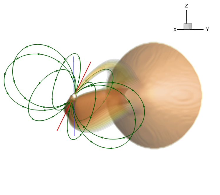
Figure 1: The flow structure in a typical polar. Isosurfaces of logarithm density (color), magnetic field lines (lines with arrows), the magnetic axis (red line), and the rotation axis (blue line) are shown.

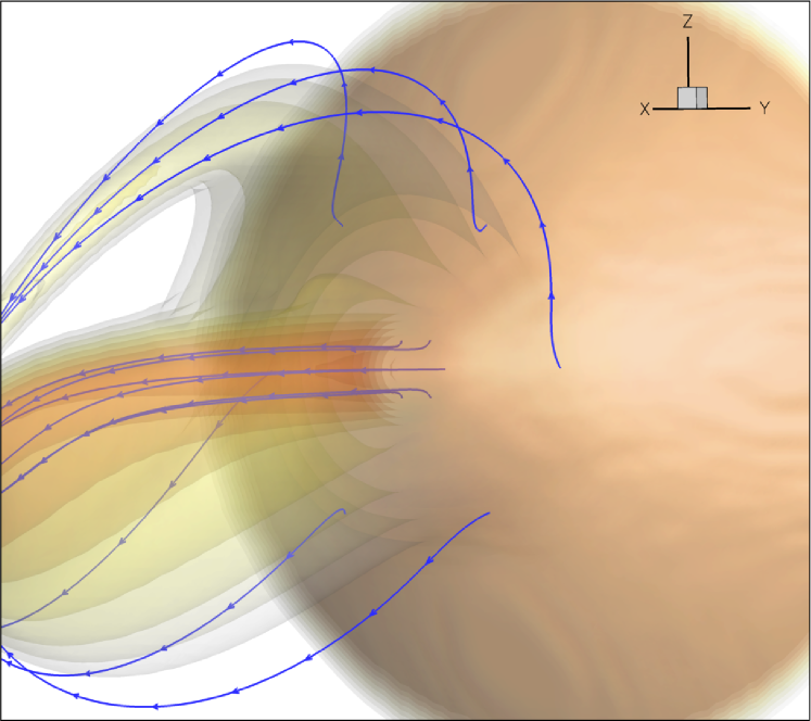
Figure 2: Flow structure in a typical polar in the region of the formation of the accretion stream. Isosurfaces of logarithm density (color) and magnetic field lines (lines with arrows) are shown.

The 3D structure of the flow is shown in Figs. 1 and 2. Figure 1 demonstrates the full pattern of the material flow from the donor surface. The computational domain includes part of the donor Roche lobe. The logarithm of the density is shown in color. The white sphere corresponds to the accretor surface. The rotation axis of the white dwarf is directed along the $z$ axis, marked by the blue line, and the magnetic axis is indicated by the red line. The green lines with arrows indicate the magnetic field lines. The material stream from the donor moves in a wide flow and falls onto the surface of the white dwarf at the magnetic poles, with the main stream falling onto the southern magnetic pole. The material first moves along a ballistic trajectory and then slightly deviates under action of the Coriolis force. When this material approaches the boundary of the white dwarf magnetosphere, it becomes trapped by the magnetic field and subsequently moves along the magnetic field lines. It is energetically more favorable for this material to accrete onto the southern magnetic pole, since this pole is located closer to the inner Lagrangian point. Nevertheless, some fraction of the material forms an accompanying flow moving toward the northern magnetic pole.

Figure 2 shows the computational results for the flow structure near the inner Lagrangian point. The isosurfaces of logarithm density are shown in color, and the blue lines with arrows indicate the direction of the flow lines. This figure demonstrates that the flow structure has a complex character. The main stream is formed in the immediate vicinity of the Lagrangian point, while additional streams are formed in more distant regions. The lower part of the accompanying stream flows into the main flow after some time. The upper part of the accompanying stream becomes trapped by the magnetic field of the white dwarf, and forms a separate collimated accretion stream. An analysis of the computational data shows that the mass flow in this stream is about a factor of $500$ lower than in the main stream.

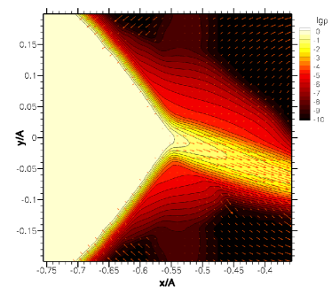
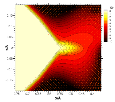
a) $z=0$	b) $y=0$
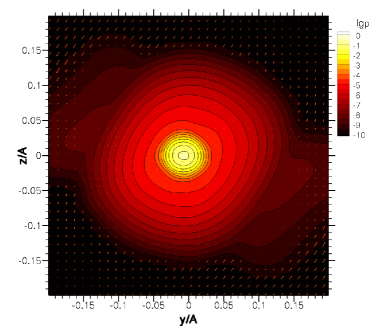
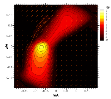
c) $x=-0.5385~{}A$	d) $x=-0.3558~{}A$

Figure 3: The distribution of the density (color) and velocity (arrows) in the $xy$ plane (upper left), $xz$ plane (upper right), $yz$ plane at $x=-0.5385~{}A$ (lower left), and $yz$ plane at $x=-0.3558~{}A$ (lower right).

Figure 3 demonstrates the flow structure in the region of formation of the stream separately in three planes: in equatorial $xy$ (upper left) and vertical $xz$ (upper right) planes, and in the $yz$ plane where $x=-0.5385~{}A$ (lower left) and $x=-0.3558~{}A$ (lower right). The distribution of the density is indicated in color, and the distribution of the velocity tangent to a given plane is marked by arrows. Analysis of the flow structure in the equatorial plane (upper left) shows that most of the material from the donor moves into the Roche lobe of the white dwarf from the vicinity of the inner Lagrangian point. The material of the accompanying streams located lower and higher L₁ has a considerably lower density. In the $xz$ plane (upper right), the bulk of the material flows downward, while a small portion continues to move straight forward, forming an additional stream. In the $yz$ plane (lower), all the material near the donor (left) moves as one flow, but, little farther from the inner Lagrangian point (right), the main stream is condensed and runs downward, while a small portion of the material forms another stream that moves upward.

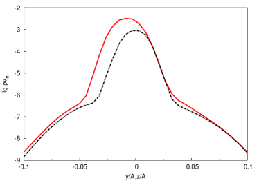
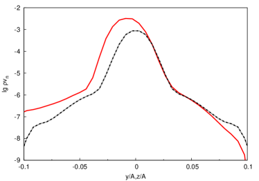
a) $B_{\text{a}}=10^{8}~{}\text{G}$	b) $B_{\text{a}}=10^{-8}~{}\text{G}$

Figure 4: Left: logarithm of the mass flow density as a function of the cross section of the accretion flow along the $y$ (red solid curve) and $z$ (black dashed curve) is for a polar with a magnetic field of $B_{\text{a}}=10^{8}~{}\text{G}$ at the accretor surface. Right: same for the gas dynamical case with the same parameters, but with the surface magnetic field $B_{\text{a}}=10^{-8}~{}\text{G}$.

Figure 4 shows profiles of the mass flow density $\rho v_{n}$ in cross sections of the accretion flow. The left plot presents profiles for the MHD case we have analyzed ($B_{\text{a}}=10^{8}~{}\text{G}$)); for comparison, the right plot shows analogous profiles for the gas dynamical case (very weak filed $B_{\text{a}}=10^{-8}~{}\text{G}$). The red and black- dashed solid curves indicate the distributions along the y and z coordinates, respectively. These plots show a central flow and ”wings” corresponding to the accompanying stream. The distribution along the y coordinate (red curve) is offset towards negative values, and has a higher maximum than the profile along the $z$ coordinate. This is due to the Coriolis force (as is clearly visible in the upper left panel of Fig. 3). An analysis of the computational data shows that the total mass flow in the main stream is almost two orders of magnitude greater than that in the accompanying streams. Furthermore, the total mass flow for the gas dynamical case is approximately 10greater than in the MHD case, due to the influence of the magnetic field on the formation of the stream, which leads to suppression of the mass transfer rate.

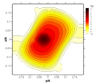
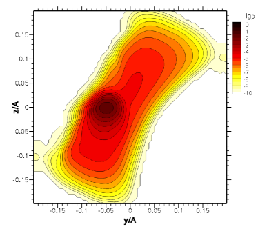
a) $x=-0.50~{}A$	b) $x=-0.42~{}A$
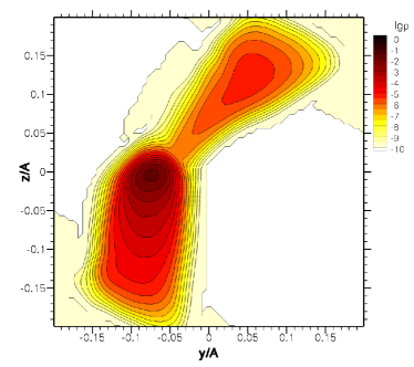
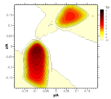
c) $x=-0.34~{}A$	d) $x=-0.26~{}A$
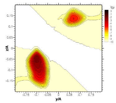
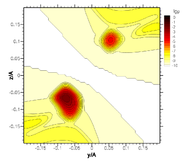
e) $x=-0.18~{}A$	f) $x=-0.10~{}A$

Figure 5: Distribution of the density (color) in $yz$ planes corresponding to different fixed values of x. Upper: $x=-0.50~{}A$ (left) and $x=-0.42~{}A$ (right); center: $x=-0.34~{}A$ (left) and $x=-0.26~{}A$ (right); lower: $x=-0.18~{}A$ (left) and $x=-0.10~{}A$ (right). Cross sections indicating the process of splitting of the stream are presented.

Figure 5 presents density distributions (color) in various cross sections of the $yz$ plane corresponding to fixed x values. The x coordinate is varied in steps of 0.08A. Recall that the coordinate of the inner Lagrangian point is $x=-0.556~{}A$. The plot for $x=-0.50~{}A$ (upper left) presents a section in the $yz$ plane in the immediate vicinity of the inner Lagrangian point. The accretion stream is extended along the axis of symmetry of the magnetic field. Its density increases towards the center, which is offset to the left along the y coordinate due to the Coriolis force. In the diagram for $x=-0.42~{}A$ (upper right), the accretion flow is even more extended. The regions of higher density are even more shifted to the left and are somewhat extended downward, while the less dense material are shifted upward. In the diagram for $x=-0.34~{}A$ (center left panel), we can clear see two dense centers: the lower one with higher density is shifted to the left and downward, while the upper one with lower density is shifted upward. A relatively thin bridge is seen between these centers. However, this bridge has disappeared in the diagram for $x=-0.26~{}A$ (center right panel). Here, the main lower flow with higher density and its accompanying upper flow with a lower density are gradually moving away from each other. In the diagram for $x=-0.18~{}A$ (lower left), the flows become collimated and their cross section narrows appreciably. Finally, in the diagram for $x=-0.10~{}A$ (lower right), we can see two separate collimated accretion flows. The lower flow corresponds to material accretion onto the southern magnetic pole of the white dwarf, and the upper flow accretion onto its northern magnetic pole.

Analysis of these diagrams leads us to conclude that the stream has a nonuniform cross section structure. The magnetic field influences less dense parts of the flow at longer distances from the white dwarf, and more dense parts of the flow at smaller distances. At $x=-0.34~{}A$, the accretion flow is beginning to split into two separate streams. This distance corresponds to the boundary of the magnetosphere for the peripheral, less dense part of the accretion stream (the ”wings” of the density profile in Fig. 4). The higher density part of the flow reaches its magnetosphere boundary after some time, and, according to this picture, should also separate onto two distinct streams due to the action of the magnetic field. However, the insufficient resolution of the grid in our computations apparently hinders our detection of this effect. In addition, these streams should again merge as they approach the southern magnetic pole.

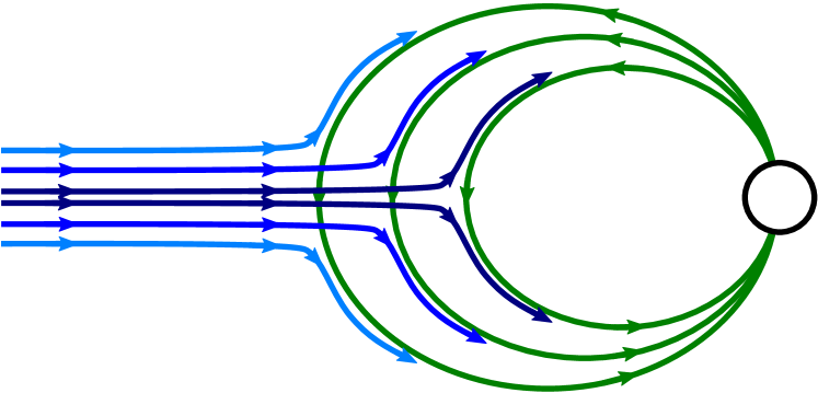
Figure 6: Schematic picture of the formation of a hierarchial magnetosphere. The circle corresponds to the white dwarf, magnetic field lines are shown by the green lines with arrows, and the blue lines of various shades indicate material flow lines, with darker shades corresponding to higher density.

Such a picture for the formation of the magnetosphere can be referred to as hierarchial. Above, we described the formation of only two hierarchial levels. However, it is clear that, in general, the number of such levels could be infinite, since the flow profile is continuous. Figure 6 shows a schematic of the formation of such a hierarchial magnetosphere. Here, the white dwarf is denoted by a circle, and its magnetic field lines are shown by the green lines with arrows. The material flow lines are indicated by the blue lines with arrows. For simplicity, we present the case for a three-layer hierarchy. Darker shades of the flow lines correspond to higher material densities. The peripheral parts of the flow (lightest shade of blue) are deflected earliest by the magnetic field and form the outer parts of the magnetosphere. More inner and denser parts of the flow (medium-dark blue) are deflected by the magnetic field somewhat later. The innermost and densest parts of the flow (darkest blue) penetrate more deeply and form the inner parts of the magnetosphere. However, all these separate flows can gradually merge near the magnetic poles into unified accretion columns or curtains. This picture for the formation of the magnetospheres in polars differs appreciably from the classical scenario, and can be used for more detailed analyses and interpretation of observations.

5 Conclusions

We have used our 3D MHD numerical model to investigate the flow structure in polars. This model is based on a modified MHD approximation, which describes the plasma dynamics in the case of strong external magnetic fields, taking into account Alfvèn wave turbulence in the presence of low magnetic Reynolds numbers. The computational domain fully encompassed the Roche lobe of the accretor, as well as part of the Roche lobe of the donor. This has enabled us to describe the formation of the outflow from the donor envelope in the vicinity of the inner Lagrangian point by a natural way using our model. Furthermore, in contrast to our preceding studies, we have used the energy equation rather than the entropy equation in this model.

We have carried out 3D MHD numerical simulations of mass transfer from the donor into the Roche lobe of the accretor. As an example, we have considered a polar with a magnetic field at the white dwarf surface of $B_{\text{a}}=10^{8}~{}\text{G}$, whose parameters correspond to SS Cyg. The structure of the formed flow was studied, paying special attention to the vicinity of the inner Lagrangian point, where the accretion flow is formed. The results of numerical simulations show that the material flowing from the donor’s envelope into the Roche lobe of the accretor forms collimated accretion flows that move toward the magnetic poles of the white dwarf. The flow formed in the vicinity of the inner Lagrangian point splits onto two separated streams due to the magnetic field. The bulk of the material is deflected downwards by the Coriolis force, and moves toward the southern magnetic pole. The less dense flow is coupled with the magnetic field lines of the accretor earlier, and drops onto the white dwarf surface in the region of its northern magnetic pole. The interaction of the accretion flow material from the donor envelope with the magnetic field leads to the formation of a hierarchial structure for the magnetosphere. The less dense (peripheral) parts of the flow are influenced by the magnetic field at longer distances from the accretor, and form the outer magnetosphere. More inner and denser parts of the flow are deflected by the magnetic field at closer distance to the accretor. The innermost and densest parts of the flow penetrate through the magnetic field and form the innermost parts of the magnetosphere. However, all these separate streams should merge near the magnetic poles and form the accretion columns or curtains at the surface of the white dwarf [41]. This scenario for the formation of hierarchial magnetospheres in polars differs appreciably from the classical picture; taking this into account can affect the results of analyses and the interpretation of observations.

References

- [1] B. Warner, Cataclysmic Variable Stars (Cambridge: Cambridge Univ. Press, 2003).
- [2] A. G. Zhilkin, D. V. Bisikalo, and A. A. Boyarchuk, Phys. Usp. 55, 115 (2012).
- [3] A. J. Norton, G. A. Wynn, R. V. Somerscales, Astrophys. J. 614, 349 (2004).
- [4] A. J. Norton, O. W. Butters, T. L. Parker, G. A. Wynn, Astrophys. J. 672, 524 (2008).
- [5] C. G. Campbell, Magnetohydrodynamics in Binary Stars (Dordrecht: Kluwer Acad. Publ., 1997).
- [6] S. H. Lubow, F. H. Shu, Astrophys. J. 198, 383 (1975).
- [7] D. V. Bisikalo, A. A. Boyarchuk, O. V. Kuznetsov, V. M. Chechetkin, Astronomy Reports. 41, 794 (1997).
- [8] D. V. Bisikalo, A. G. Zhilkin, and A. A. Boyarchuk, Gas Dynamics of Close Binary Stars (Fizmatlit, Moscow, 2013) [in Russian].
- [9] T. Tanaka, J. Comp. Phys. 111, 381 (1994).
- [10] K. G. Powell, P. L. Roe, T. J. Linde, T. I. Gombosi, D. L. De Zeeuw, J. Comput. Phys. 154, 284 (1999).
- [11] F. Giovannelli, S. Gaudenzi, C. Rossi, A. Piccioni, Acta Astronomica. 33, iss. 2, 319 (1983).
- [12] L. D. Landau and E. M. Lifshitz, Course of Theoretical Physics, Vol. 8: Electrodynamics of Continuous Media (Fizmatlit, Moscow, 2003; Pergamon, New York, 1984).
- [13] V. M. Lipunov, Astrophysics of Neutron Stars (Nauka, Moscow, 1987; Springer, Heidelberg, 1992).
- [14] L. D. Landau and E. M. Livshitz, Course of Theoretical Physics, Vol. 2: The Classical Theory of Fields (Fizmatlit, Moscow, 2006; Pergamon, Oxford, 1975).
- [15] D. P. Cox and E. Daltabuit, Astrophys. J. 167, 113 (1971).
- [16] A. Dalgarno and R. A. McCray, Ann. Rev. Astron. Astrophys. 10, 375 (1972).
- [17] J. C. Raymond, D. P. Cox, and B. W. Smith, Astrophys. J. 204, 290 (1976).
- [18] L. Spitzer, Physical Processes in the Interstellar Medium (Wiley, New York, 1978).
- [19] A. G. Zhilkin and D. V. Bisikalo, Astron. Rep. 53, 436 (2009).
- [20] A. G. Zhilkin and D. V. Bisikalo, Astron. Rep. 54, 1063 (2010).
- [21] A. G. Zhilkin and D. V. Bisikalo, Astron. Rep. 54, 840 (2010).
- [22] M. M. Romanova, G. V. Ustyugova, A. V. Koldoba, J. V. Wick, and R. V. E. Lovelace, Astrophys. J. 595, 1009 (2003).
- [23] G. S. Bisnovatyi–Kogan, S. G. Moiseenko, Astrophysics. 59, 1 (2016).
- [24] E. P. Kurbatov, A. G. Zhilkin, and D. V. Bisikalo, Phys. Usp. 60, 798 (2017).
- [25] S. I. Braginskii, Sov. Phys. JETP 10, 1005 (1960).
- [26] V. E. Zakharov, Zh. Prikl. Mekh. Tekh. Fiz. 1, 14 (1965).
- [27] P. S. Iroshnikov, Sov. Astron. 7, 566 (1963).
- [28] R. H. Kraichnan, Phys. Fluids. 8, 575 (1965).
- [29] A. G. Zhilkin, D. V. Bisikalo, P. A. Mason, Astronomy Reports 56, 257 (2012).
- [30] D. V. Bisikalo, A. G. Zhilkin, P. V. Kaygorodov, V. A. Ustyugov, and M. M. Montgomery, Astron. Rep. 57, 327 (2013).
- [31] V. A. Ustyugov, A. G. Zhilkin, and D. V. Bisikalo, Astron. Rep. 57, 811 (2013).
- [32] P. B. Isakova, A. G. Zhilkin, and D. V. Bisikalo, Astron. Rep. 59, 843 (2015).
- [33] A. M. Fateeva, A. G. Zhilkin, and D. V. Bisikalo, Astron. Rep. 60, 87 (2015).
- [34] P. B. Isakova, N. R. Ikhsanov, A. G. Zhilkin, D. V. Bisikalo, and N. G. Beskrovnaya, Astron. Rep. 60, 498 (2016).
- [35] P. B. Isakova, A. G. Zhilkin, D. V. Bisikalo, A. N. Semena, and M. G. Revnivtsev, Astron. Rep. 61, 560 (2017).
- [36] S. D. Drell, H. M. Foley, and M. A. Ruderman, J. Geophys. Res., 70, 3131 (1965).
- [37] A. V. Gurevich, A. L. Krylov, and E. N. Fedorov, Sov. Phys. JETP 48, 1074 (1978).
- [38] R. R. Rafikov, A. V. Gurevich, and K. P. Zybin, J. Exp. Theor. Phys. 88, 297 (1999).
- [39] D. A. Frank-Kamenetskii, Lectures on Plasma Physics (Atomizdat, Moscow, 1968) [in Russian].
- [40] F. F. Chen, Introduction to Plasma Physics (Springer, New York, 2012).
- [41] A. N. Semena and M. G. Revnivtsev, Astron. Lett. 38, 321 (2012).