Surface super-roughening driven by spatiotemporally correlated noise

Abstract

We study the simple, linear, Edwards-Wilkinson equation that describes surface growth governed by height diffusion in the presence of spatiotemporally power-law decaying correlated noise. We analytically show that the surface becomes super-rough when the noise correlations spatio/temporal range is long enough. We calculate analytically the associated anomalous exponents as a function of the noise correlation exponents. We also show that super-roughening appears exactly at the threshold point where the local slope surface field becomes rough. In addition, our results indicate that the recent numerical finding of anomalous kinetic roughing of the Kardar-Parisi-Zhang model subject to temporally correlated noise may be inherited from the linear theory.

I Introduction

Surfaces and interfaces driven by random noise often become dynamically rough and give rise to scale-invariant profiles. Examples can be found in surfaces formed by particle deposition processes in thin-film growth (e.g., molecular-beam epitaxy, sputtering, electrodeposition, and chemical-vapor deposition) Barabási and Stanley (1995); Krug (1997), advancing fracture cracks Alava et al. (2006), and fluid-flow depinning in disordered media Alava et al. (2004), among many others.

A surface $h(\mathbf{x},t)$ is said to be scale-invariant if its statistical properties remain unchanged after re-scaling of space and time according to the transformation $h(\mathbf{x},t)\to b^{\alpha}h(b\,\mathbf{x},b^{1/z}\,t)$, for any scaling factor $b>1$ and a certain choice of critical exponents $\alpha$ and $z$ Barabási and Stanley (1995); Krug (1997). Scale-invariant surface growth is associated with symmetries Hentschel (1994). Indeed, if the dynamical evolution of the surface height $h(\mathbf{x},t)$ satisfies a set of fundamental symmetries (rotation, translation in $\mathbf{x}$, time invariance, etc), including the fundamental shift symmetry $h\to h+c$, where $c$ is a constant, then scale-invariant behaviour is expected without fine tuning of any external parameters or couplings.

Scale invariance implies that the local height-height correlations exhibit power-law behaviour:

$$\langle\overline{[h(\mathbf{x},t)-h(\mathbf{x}+\mathbf{l},t)]^{2}}\rangle^{1/2}=l^{\alpha}{\cal G}(l/t^{1/z}),$$ (1)

where overbar denotes average over all $\mathbf{x}$, brackets denote average over realizations, and the critical exponents $\alpha$ and $z$ are the roughening and dynamic exponents, respectively. The scaling function ${\cal G}(u)$ becomes constant for $u\ll 1$, and decays as $\sim u^{-\alpha}$ for $u\gg 1$. A similar scaling describes the global surface width, $W(L,t)=\langle\overline{[h(\mathbf{x},t)-\overline{h}(t)]^{2}}\rangle^{1/2}$, which is expected to scale as $W(L,t)=L^{\alpha}{\cal F}(L/t^{1/z})$, where $\cal F$ is a scaling function with the same asymptotic behaviour as $\cal G$ in (1). Therefore, in the stationary regime $t\gg L^{z}$, we have $W_{\mathrm{stat}}(L)\sim L^{\alpha}$. This scaling picture of kinetically roughened surfaces is usually termed Family-Vicsek (FV) ansatz Family and Vicsek (1985) and has shown to be tremendously successful to describe surface growth in a variety of theoretical models and experiments Barabási and Stanley (1995); Krug (1997).

Nowadays, it has become clear that there exist scale-invariant surface growth models where the above standard FV scaling fails, leading to distinctly different scaling functions for the local and global surface fluctuations. Specifically, the local height-height correlation function takes the form (1) but with an anomalous scaling function given by López et al. (1997a, b)

$${\cal G}_{\mathrm{A}}(u)\sim\left\{\begin{array}[]{lcl}u^{\alpha_{\mathrm{loc}}-\alpha}&{\rm if}&u\ll 1\\ u^{-\alpha}&{\rm if}&u\gg 1,\end{array}\right.$$ (2)

for $t\ll L^{z}$, instead of the standard form (note that standard FV scaling is recovered for $\alpha=\alpha_{\mathrm{loc}}$). Therefore, for intermediate times, $l^{z}\ll t\ll L^{z}$, one has $\langle\overline{[h(\mathbf{x},t)-h(\mathbf{x}+\mathbf{l},t)]^{2}}\rangle^{1/2}\sim l^{\alpha_{\mathrm{loc}}}\,t^{\kappa}$, where $\kappa=(\alpha-\alpha_{\mathrm{loc}})/z$. While the local surface fluctuations only saturate at times $t\gg L^{z}$, when they become time independent, and one finds $\sim l^{\alpha_{\mathrm{loc}}}L^{\alpha-\alpha_{\mathrm{loc}}}$. This leads to the existence of an independent local roughness exponent $\alpha_{\mathrm{loc}}$ that characterizes the local interface fluctuations and differs from the global roughness exponent $\alpha$ obtained by, for instance, the global width. This phenomenon is referred to as anomalous roughening and has received much attention in the last few years because its commonness in experiments López and Schmittbuhl (1998); Morel et al. (1998); Myllys et al. (2000); Huo and Schwarzacher (2001); Soriano et al. (2002, 2005); Auger et al. (2006); Planet et al. (2007); Cordoba-Torres et al. (2008); Sana et al. (2017); Orrillo et al. (2017); Meshkova et al. (2018); Planet et al. (2018).

Current theoretical knowledge has firmly established Ramasco et al. (2000) that, indeed, the existence of power-law scaling of the correlation functions (i.e., scale invariance) does not determine a unique dynamic scaling form of the correlation functions. Ramasco et al. Ramasco et al. (2000) theory of generic dynamic scaling of surface growth predicts the existence of four possible scaling scenarios. First, the standard FV scaling behavior described above. Second, there are super-rough processes, $\alpha>1$, for which $\alpha_{\mathrm{loc}}=1$ always. Third, there are intrinsically anomalous roughened surfaces, for which the local roughness $\alpha_{\mathrm{loc}}<1$ is actually an independent exponent and $\alpha$ may take values larger or smaller than one depending on the universality class (see López et al. (2005); Ramasco et al. (2000) and references therein). Finally, the fourth scaling scenario is associated with faceted surfaces, where spatio-temporal correlations take a different form, also explained by the generic dynamic scaling theory of Ramasco et al. Ramasco et al. (2000).

The natural question that arises is what kind of interactions (symmetries, form of the nonlinearities, conservation laws, non-locality, etc) are required for anomalous roughening to occur in surface growth?. There are theoretical arguments López et al. (2005) that strongly suggest that local models of surface growth driven by white noise cannot exhibit intrinsic anomalous roughening, but super-roughening can occur in models with some conserved dynamics. Interestingly, a recent numerical study Alés and López (2019) of the Kardar-Parisi-Zhang (KPZ) equation with long temporally correlated noise has found anomalous scaling (associated with facet formation) above some critical threshold of the noise correlator index. This indicates that strong noise correlations may also lead to anomalous roughening.

In this paper we show that, even in the simplest local linear growth model, standard FV scaling can break down if the noise fluctuations are long-term and/or long-range correlated. We study the simplest, linear, scale-invariant growth model, that only takes into account surface diffusion— the so-called Edwards-Wilkinson (EW) equation Edwards and Wilkinson (1982)— in the presence of long-time and/or long-range correlated noise. We show analytically that when spatial/temporal range of the noise correlations is long enough the surface becomes super-rough with a local roughness exponent $\alpha_{\mathrm{loc}}=1$ and a global roughness exponent $\alpha>1$, which value depends on the degree of correlation. We also show that super-roughening is associated with the local surface slope $\nabla h$ becoming rough itself, in agreement with an existing theoretical conjecture López et al. (2005). We compare our analytical results with the numerical integration of the model in the case of temporally correlated noise.

Our results shed some light into a recent numerical study Alés and López (2019) of the KPZ equation with long-term correlated noise. In that study it was found that the scaling of the KPZ surface becomes anomalous (and faceted) above some critical threshold of the noise correlator index, which was numerically estimated to be $\theta_{c}\approx 0.25$. Here we show that the critical threshold $\theta_{c}=1/4$ appears already in the linear theory as the correlation strength above which the surfaces of the linear model become super-rough.

Theoretical models exhibiting anomalous scaling that are suited for full analytical treatment are scarce in the literature, therefore, most examples have come from either simulations, experiments or scaling approximations. Hence, exact analytical results on anomalous behavior are very welcomed.

II Theoretical analysis

In kinetic surface roughening the EW Edwards and Wilkinson (1982) equation plays a central role as the simplest, linear, equilibrium model exhibiting scale-invariant behavior. The model describes surface growth governed by height diffusion (linear elasticity) subject to noisy thermal-like fluctuations. In $d=1+1$ dimensions it can be written as

$$\partial_{t}h(x,t)=\nu\nabla^{2}h+\eta(x,t),$$ (3)

where the field $h(x,t)$ represents the height of the surface at time $t$ and position $x$, $\nu$ is the surface tension, and the noise term $\eta(x,t)$ is usually Gaussian and uncorrelated in space and time.

Here we consider the EW equation with long-time and/or long-range correlated, instead of thermal uncorrelated noise. For simplicity, we analyse only the one-dimensional case, although it is easily generalizable to larger dimensions. The stochastic term has long-term correlations with $\langle\eta(x,t)\rangle=0$ and

$$\langle\eta(x,t)\eta(x^{\prime},t^{\prime})\rangle=2D|t-t^{\prime}|^{-(1-2\theta)}|x-x^{\prime}|^{-(1-2\rho)},$$ (4)

being $D$ the noise amplitude, and $\rho$, $\theta\in[0,1/2)$ are the spatial and temporal correlation exponents, respectively, describing the spatial and temporal extent of correlations. This problem was already studied by Pang and Tzeng Pang and Tzeng (2004) and the scaling functions were calculated using real space methods. Here we use a much more transparent calculation of the complete spectral density function (structure factor) from which the scaling functions and exponents are immediately obtained, including the roughness exponent of the local slope field.

The noise correlator (4) can be written in Fourier space as

$$\langle\hat{\eta}(k,\omega)\hat{\eta}(k^{\prime},\omega^{\prime})\rangle=2D\,|k|^{-2\rho}w^{-2\theta}\delta(k+k^{\prime})\delta(\omega+\omega^{\prime}).$$ (5)

In the limit, $\rho$, $\theta\to 0$ one recovers the case of uncorrelated noise.

In Fourier space the solution of the EW model, Eq. (3), is given by

$$\hat{h}(k,\omega)=\frac{\hat{\eta}(k,\omega)}{\nu k^{2}-i\omega},$$ (6)

from which it is possible to obtain the structure factor $\Phi(k,\omega)=\langle|\hat{h}(k,\omega)|^{2}\rangle$ by multiplying the expression (6) by its complex conjugate and making a statistical average over the noise; where the correlator (5) of the stochastic term is used. The spectral power density is then given by

$$\Phi(k,\omega)=\frac{2Dk^{-2\rho}\omega^{-2\theta}}{\nu^{2}k^{4}+\omega^{2}}.$$ (7)

By transforming back to real time, inverting the Fourier transform in frequencies space, we obtain the exact two-times structure factor

$$\Phi(k,\Delta t)=\frac{D}{\nu^{2}2^{-1/2-2\theta}}k^{-2-2\rho-4\theta}f(\nu k^{2}\Delta t),$$ (8)

where the scaling function is found to take the form

$$f(u) =4^{\theta}e^{-u}$$

$$-u^{1+2\theta}\frac{{}_{1}F_{2}\{1;1+\theta,\frac{3}{2}+\theta;\frac{u^{2}}{4}\}}{\Gamma(1+\theta)\Gamma(\frac{3}{2}+\theta)},$$

where $\Gamma$ is the Complete Gamma function and ${}_{1}F_{2}$ the Generalized Hypergeometric function Olver et al. (2010). The global roughness exponent $\alpha$ can be immediately obtained from the power-law behavior of Eq. (8), which has a tail given by $k^{-\gamma}$, being $\gamma=2\alpha+1$. The dynamic exponent is given by the argument of the scaling function $u=\nu k^{2}\Delta t$, which describes a crossover at momenta $k=(\nu\Delta t)^{1/z}$, with $z=2$. Therefore, the following exact exponents are obtained:

$$\alpha=1/2+\rho+2\,\theta\;\;\;\mathrm{and}\;\;\;z=2.$$ (9)

Note that the global roughness exponent is greater than unity for $\rho+2\theta>1/2$. This already indicates the surface will break standard FV scaling in this region and we expect to have a different local roughness exponent $\alpha_{\mathrm{loc}}\neq\alpha$.

In order to calculate $\alpha_{\mathrm{loc}}$ for this model we resort to the theory developed in Ref. López (1999), which allows us to compute the local scaling properties of growth models from the dynamics of the local slope field $\Upsilon(x,t)\equiv\nabla h(x,t)$.

From the EW dynamics in Eq. (3) we have that the local slope field time evolution is given by

$$\partial_{t}\Upsilon(x,t)=\nu\nabla^{2}\Upsilon(x,t)+\eta^{c}(x,t),$$

where $\eta^{c}$ is a correlated and conserved noise with

$$\langle\eta^{c}(x,t)\eta^{c}(x^{\prime},t^{\prime})\rangle=-2D\,\nabla^{2}|x-x^{\prime}|^{2\rho-1}|t-t^{\prime}|^{2\theta-1}.$$

Being a linear equation we can follow the same procedure as before to calculate the spectral power density and we have

$$\langle\hat{\Upsilon}(k,\omega)\hat{\Upsilon}(-k,-\omega)\rangle=2D\,\frac{k^{2(1-\rho)}\,\omega^{-2\theta}}{\nu^{2}k^{4}+\omega^{2}},$$

where the extra $k^{2}$ in the numerator comes from the correlator of the conserved noise, but otherwise the formula is the same as Eq. (7). Inverting the Fourier transform in frequencies and by a similar calculation as before we arrive at the dynamic exponent $z=2$ (being a linear model, both $h$ and $\nabla h$ should have the same dynamic exponent) and the roughness exponent

$$\hat{\alpha}=-1/2+2\theta+\rho,$$ (10)

for the local slope field $\Upsilon(x,t)$. Note that, for $\hat{\alpha}>0$, the local slope field is a rough surface itself; marking the existence of anomalous roughening of the original surface $h(x,t)$ López (1999). Accordingly, we expect the local width of $h$ to scale anomalously as $w(l,t)\sim l^{\alpha_{\mathrm{loc}}}\,t^{\kappa}$ for scales $l^{z}<t<L^{z}$ when $\hat{\alpha}>0$ López (1999), instead of being $w(l,t)\sim l^{\alpha}$ as corresponds to FV scaling. The anomalous time exponent corresponds to the time growth of the slope field fluctuations $\kappa=\tilde{\alpha}/z$ and it is also related to the local roughness exponent through the expression $\alpha_{\mathrm{loc}}=\alpha-\kappa z$, as described by the general theory in Ref. López (1999). These two scaling relationships allow us to obtain $\alpha_{\mathrm{loc}}$ from the time growth exponent, $\kappa$, of the local slope field.

Replacing (10) in the expression $\kappa=\hat{\alpha}/z$, we obtain

$$\kappa=\frac{-1/2+2\theta+\rho}{2}$$ (11)

when $\hat{\alpha}>0$ and $\kappa=0$ otherwise. The local roughness exponent $\alpha_{\mathrm{loc}}$ follows immediately by using (9) and (11)

$$\alpha_{\mathrm{loc}}=\alpha-\kappa z=\left\{\begin{array}[]{lcl}1/2+2\theta+\rho&\mathrm{if}&2\theta+\rho\leq 1/2\\ 1&\mathrm{if}&2\theta+\rho>1/2\end{array}\right.$$ (12)

Therefore, we find two branches for the value of the local roughness exponent $\alpha_{\mathrm{loc}}$ depending on the noise correlation indexes, $\rho$ and $\theta$. On the one hand, the standard FV scaling branch, for $2\theta+\rho\leq 1/2$, where $\hat{\alpha}=\kappa=0$ and we have $\alpha=\alpha_{\mathrm{loc}}=1/2+2\theta+\rho$. On the other hand, the anomalous branch, for $2\theta+\rho>1/2$, where the local slope field becomes rough ($\hat{\alpha}>0$) and $\alpha=1/2+2\theta+\rho>1$ and $\alpha_{\mathrm{loc}}=1$, which corresponds to super-roughening.

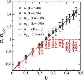
Figure 1: Global $\alpha$ and local $\alpha_{\mathrm{loc}}$ roughness exponents obtained from numerical integration of the EW equation for a temporally correlated noise with index $\theta$. Above the threshold value $\theta_{c}=0.25$ the behaviour of the global and local roughness exponents split apart, as predicted by theory, Eqs. (12) and (9).

III Numerical results

We now check our analytical results with the numerical integration of the EW dynamics with long-time correlated noise. We focus on the case of temporally correlated noise for which $\rho=0$ and the index $\theta$ is varied in the interval $\theta\in[0,1/2]$. Stochastic integration of the EW model was carried out by using a standard Euler-Maruyana Milstein (1994) scheme, with a discretization of Eq. (3) given by

$$h_{i}(t+\Delta t)=h_{i}(t)+\Delta t\,L_{i}(t)+\Delta t\,\eta_{i}(t),$$

being $\Delta t$ the temporal step and $\eta_{i}(t)$ the noise at position $i$ and time $t$. The Laplacian term is discretized as

$$L_{i}(t)=\frac{h_{i+1}(t)+h_{i-1}(t)-2h_{i}(t)}{\left(\Delta x\right)^{2}}.$$

where lattice constant is set to $\Delta x=1$ and the time step $\Delta t=10^{-3}$. Periodic boundary conditions were used in all our simulations. The generation of noise with the desired correlations has been carried out using the Gaussian noise fractional technique developed by Mandelbrot Mandelbrot (1971), which has proven to be very efficient and precise Alés and López (2019); Lam et al. (1992) for systems similar to ours. Statistical averages over 100 independent runs were taken for the larger system size and more for smaller ones. We studied system sizes $L=1024$, $2048$ and $4096$ and the surface evolution was followed up to times of the order $t=10^{6}$, for which the system was already in the stationary state.

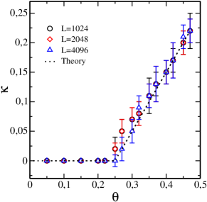
Figure 2: Local growth exponent $\kappa$ for EW with temporally correlated noise and the analytical prediction, Eq. (11). The value of $\kappa$ is positive above $\theta_{\mathrm{c}}>0.25$.

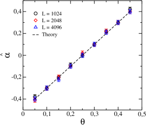
Figure 3: Roughness exponent of the local slope field $\Upsilon(x,t)$ as a function of the noise correlation index $\theta$. Note that $\hat{\alpha}$ becomes positive for $\theta>\theta_{c}=1/4$, marking the point above which the slope surface field becomes rough.

We obtained the global roughness exponent numerically from the equal-times spectral density, $\langle|\hat{h}(k,t)|^{2}\rangle$, for different values of the temporal noise correlation exponent $\theta$ within the interval $[0,1/2)$. We find that, in the stationary regime, the spectral density exhibits scaling behaviour $\langle|\hat{h}(k,t\gg L^{z})|^{2}\rangle\sim k^{-(2\alpha+1)}$, where $\alpha$ is the global roughness exponent. We also computed the local roughness exponent from the data collapse of $l^{-\alpha}\langle\overline{[h(\mathbf{x},t)-h(\mathbf{x}+\mathbf{l},t)]^{2}}\rangle^{1/2}$ vs. $l/t^{1/z}$, for a fixed system size $L$, according to the scaling behaviour in Eq. (2). This gives us independent measurements of $z$, $\alpha$, and produces an estimate of $\alpha_{\mathrm{loc}}$ from the power fit of the scaling function asymptote, $\sim(l/t^{1/z})^{2(\alpha_{\mathrm{loc}}-\alpha)}$, for $l/t^{1/z}\ll 1$. These results are summarized in Fig. 1, where one can observe that $\alpha=\alpha_{\mathrm{loc}}$ for a correlation index $\theta<1/4$, while the roughness exponents split above that threshold when $\alpha_{\mathrm{loc}}$ gets values around $0.9$. The figure also shows the theoretical prediction given by Eqs. (9) and (12).

We also measured the anomalous time exponent $\kappa$ from the time-growth of the local slope fluctuations, $\langle\overline{(\nabla h)^{2}}\rangle\sim t^{2\kappa}$. Alternatively, $\kappa$ could also be measured from the time behaviour of the height-height correlation at a fixed scale $l\ll L$, $\overline{[h(\mathbf{x},t)-h(\mathbf{x}+\mathbf{l},t\gg L^{z})]^{2}}\rangle\sim l^{2\alpha_{\mathrm{loc}}}\,t^{2\kappa}$ Ramasco et al. (2000). In Fig. 2 we show our results for $\kappa$ as a function of $\theta$ together with the analytical prediction. We observe that, in agreement with the theoretical prediction, $\kappa=0$ for $\theta<1/4$ and follows Eq. (11) above that point.

Finally, we measured the roughness exponent of the local slope field $\Upsilon(x,t)$ by computing the spectral density in the stationary state, $\langle|\hat{\Upsilon}(k,t\gg L^{z})|^{2}\rangle\sim k^{-(2\hat{\alpha}+1)}$, from here we obtained the roughness exponent $\hat{\alpha}$ for the slope field. Figure 3 summarizes our numerical results as the noise correlation index $\theta$ is varied.

IV Conclusions

We have studied the simple, linear, EW dynamics of surface growth in the presence of noise with spatio-temporal power-law decaying correlations. We have found analytically that the surface becomes super-rough ($\alpha>1$ and $\alpha_{\mathrm{loc}}=1$) for correlation noise indexes satisfying $\rho+2\theta>1/2$. Our calculation in Fourier space is more transparent and much simpler than an earlier method Pang and Tzeng (2004) based on a direct calculation of the height-height correlation in real space. Taking advantage of the simplicity of the calculation in Fourier space, we also derived an exact prediction for the anomalous time exponent $\kappa$ as a function of the noise correlation by resorting to studying the dynamics of the local slope surface. This technique allowed us to study the roughness exponent $\hat{\alpha}$ of the surface slope field and show analytically that the appearance of the super-roughening regime of the EW surface is associated with the slope field becoming rough itself, i.e. $\hat{\alpha}>0$, in agreement with existing theory López et al. (2005). In addition, we compared our theoretical predictions with a numerical integration of the EW equation in the case of temporally correlated noise.

In the particular case of temporal correlated noise ($\rho=0$), our results lead to the exact threshold $\theta_{\mathrm{c}}=1/4$, which is very close, if not identical, to the critical value recently found numerically for the appearance of anomalous scaling in the nonlinear KPZ equation Alés and López (2019). It is remarkable, and not fully understood yet, that the critical threshold for anomalous kinetic roughening in KPZ with temporally correlated noise appears to be inherited from the linear theory.

References

- Barabási and Stanley (1995) A.-L. Barabási and H. E. Stanley, Fractal Concepts in Surface Growth (Cambridge University Press, Cambridge, 1995) .
- Krug (1997) J. Krug, Adv. Phys. 46, 139 (1997).
- Alava et al. (2006) M. J. Alava, P. K. V. V. Nukala, and S. Zapperi, Adv. Phys. 55, 349 (2006).
- Alava et al. (2004) M. Alava, M. Dubé, and M. Rost, Adv. Phys. 53, 83 (2004).
- Hentschel (1994) H. G. E. Hentschel, J. Phys. A: Math. Gen. 27, 2269 (1994).
- Family and Vicsek (1985) F. Family and T. Vicsek, J. Phys. A: Math. Gen. 18, L75 (1985).
- López et al. (1997a) J. M. López, M. A. Rodríguez, and R. Cuerno, Physica A 246, 329 (1997a).
- López et al. (1997b) J. M. López, M. A. Rodriguez, and R. Cuerno, Phys. Rev. E 56, 3993 (1997b).
- López and Schmittbuhl (1998) J. M. López and J. Schmittbuhl, Phys. Rev. E 57, 6405 (1998).
- Morel et al. (1998) S. Morel, J. Schmittbuhl, J. M. López, and G. Valentin, Phys. Rev. E 58, 6999 (1998).
- Myllys et al. (2000) M. Myllys, J. Maunuksela, M. J. Alava, T. Ala-Nissila, and J. Timonen, Phys. Rev. Lett. 84, 1946 (2000).
- Huo and Schwarzacher (2001) S. Huo and W. Schwarzacher, Phys. Rev. Lett. 86, 256 (2001).
- Soriano et al. (2002) J. Soriano, J. J. Ramasco, M. A. Rodríguez, A. Hernández-Machado, and J. Ortín, Phys. Rev. Lett. 89, 026102 (2002).
- Soriano et al. (2005) J. Soriano, A. Mercier, R. Planet, A. Hernández-Machado, M. A. Rodríguez, and J. Ortín, Phys. Rev. Lett. 95, 104501 (2005).
- Auger et al. (2006) M. A. Auger, L. Vázquez, R. Cuerno, M. Castro, M. Jergel, and O. Sánchez, Phys. Rev. B 73, 045436 (2006).
- Planet et al. (2007) R. Planet, M. Pradas, A. Hernández-Machado, and J. Ortín, Phys. Rev. E 76, 056312 (2007).
- Cordoba-Torres et al. (2008) P. Cordoba-Torres, I. N. Bastos, and R. P. Nogueira, Phys. Rev. E 77, 031602 (2008).
- Sana et al. (2017) P. Sana, L. Vázquez, R. Cuerno, and S. Sarkar, J. Phys. D: Appl. Phys. 50, 435306 (2017).
- Orrillo et al. (2017) P. A. Orrillo, S. N. Santalla, R. Cuerno, L. Vázquez, S. B. Ribotta, L. M. Gassa, F. J. Mompean, R. C. Salvarezza, and M. E. Vela, Sci. Rep. 7, 17997 (2017).
- Meshkova et al. (2018) A. S. Meshkova, S. A. Starostin, M. C. M. van de Sanden, and H. W. de Vries, J. Phys. D: Appl. Phys. 51, 285303 (2018).
- Planet et al. (2018) R. Planet, J. M. López, S. Santucci, and J. Ortín, Phys. Rev. Lett. 121, 034101 (2018).
- Ramasco et al. (2000) J. J. Ramasco, J. M. López, and M. A. Rodríguez, Phys. Rev. Lett. 84, 2199 (2000).
- López et al. (2005) J. M. López, M. Castro, and R. Gallego, Phys. Rev. Lett. 94, 166103 (2005).
- Alés and López (2019) A. Alés and J. M. López, Phys. Rev. E 99, 062139 (2019).
- Edwards and Wilkinson (1982) S. F. Edwards and D. R. Wilkinson, Proc. R. Soc. London, Ser. A 381, 17 (1982).
- Pang and Tzeng (2004) N.-N. Pang and W.-J. Tzeng, Phys. Rev. E 70, 011105 (2004).
- Olver et al. (2010) F. W. J. Olver, D. W. Lozier, R. F. Boisvert, and C. W. Clark, eds., NIST handbook of mathematical functions (Cambridge University Press, 2010).
- López (1999) J. M. López, Phys. Rev. Lett. 83, 4594 (1999).
- Milstein (1994) G. N. Milstein, Numerical integration of stochastic differential equations, Vol. 313 (Springer Science & Business Media, 1994).
- Mandelbrot (1971) B. B. Mandelbrot, Water Resour. Res. 7, 543 (1971).
- Lam et al. (1992) C.-H. Lam, L. M. Sander, and D. E. Wolf, Phys. Rev. A 46, R6128 (1992).