Conditional generation of multiphoton-subtracted squeezed vacuum states: loss consideration and operator description

Abstract

In terms of the characteristic functions of the quantum states, we present a complete operator description of a lossy photon-subtraction scheme. Feeding a single-mode squeezed vacuum into a variable beam splitter and counting the photons in one of the output channels, a broad class of multiphoton-subtracted squeezed vacuum states (MSSVSs) can be generated in other channel. Here the losses are considered in the beginning and the end channels in the circuit. Indeed, this scheme has been discussed in Ref. [Phys. Rev. A 100, 022341 (2019)]. However, different from the above work, we give all the details of the optical fields in all stages. In addition, we present the analytical expressions and numerical simulations for the success probability, the quadrature squeezing effect, photon-number distribution and Wigner function of the MSSVSs. Some interesting results effected by the losses are obtained.

Keywords: Quantum state engineering, Photon-subtracted Operation, Conditional measurement, Loss channel, Characteristic function.

PACS: 42.50.Dv; 03.65.Ta

I Introduction

A key requirement for many quantum protocols is to use specific quantum states of light as a resource for information processing1 . These quantum states can be divided into Gaussian and non-Gaussian cases2 . For example, the coherent state and the single-mode squeezed vacuum state are the typical Gaussian state, which are applied in many tasks3 . However, various important protocols for quantum enhanced information processing cannot be performed when restricted to Gaussian states4 . Thus, it is necessary to introducing non-Gaussianity into an optical system. In recent years, many non-Gaussian quantum states have been used as resources for useful quantum information processing tasks 5 ; 6 . Therefore, a crucial goal for experimental quantum optics is to prepare high-quality non-Gaussian quantum states.

Photon-subtraction operation is just a useful way to conditionally manipulate a non-Gaussian state of the optical field, which has been shown to enhance entanglement7 ; 8 and teleportation fidelity9 . Theoretically, subtraction of $m$ photons from a single-mode quantum state $\left|\psi\right\rangle$ can be expressed as $a^{m}\left|\psi\right\rangle$, where $a$ is the photon annihilation operator9-1 . Experimentally, such photon-subtracted state can be implemented by transmitting $\left|\psi\right\rangle$ through a beam splitter and detecting the output of the beam splitter with photon number resolving detector9-2 . Studies have shown that photon subtraction on a single-mode squeezed vacuum state yields optical coherent-state superposition10 or Schrodinger-cat-like states11 .

As a matter of fact, the loss is unavoidable in the propagating channel of light beams. It is necessary to analyze and control the effect of loss in the quantum protocols12 ; 13 . Very recently, Quesada et al. considered some schemes of preparing conditional non-Gaussian states in the presence of photon loss. Among them, the photon-subtraction scheme is more attracted our attention14 . In the present paper, we shall give a description for the same scheme in terms of the characteristic function (CF) of the quantum states involved. The CF of density operator $\rho$ can be defined as $\chi_{\rho}\left(\alpha\right)=\mathrm{Tr}[\rho D\left(\alpha\right)]$, i.e. the expectation value of the Weyl displacement operator $D\left(\alpha\right)=\exp\left(\alpha a^{{\dagger}}-\alpha^{\ast}a\right)$ 15 . One main tool in dealing with optical field is the Weyl expansion of the density operator, that is,

$$\rho=\int\frac{d^{2}\alpha}{\pi}\chi_{\rho}(\alpha)D\left(-\alpha\right),$$ (1)

which means that the function $\chi_{\rho}(\alpha)$ uniquely determines the density operator $\rho$ 16 ; 17 . Another tool in deriving input-output relation of loss channel $L\left(\eta\right)$ (with loss factor $\eta\in[0,1]$) is that the output density operator $\rho_{out}$ can be expressed as the integration form of the input CF $\chi_{\rho_{in}}\left(\alpha\right)$, i.e.

$$\rho_{out}=\int\frac{d^{2}\alpha}{\pi}\chi_{\rho_{in}}(\sqrt{1-\eta}\alpha)D\left(-\alpha\right)e^{-\frac{1}{2}\eta\left|\alpha\right|^{2}},$$ (2)

which describes that $\rho_{in}$ evolutes into $\rho_{out}$ through loss channel. This equation has been derived in our previous work18 .

The paper is organized as follows. In Sec.2, we introduce the density operator description of generating such state. Here we shall give the conceptual scheme and decompose the whole circuit into five stages, whose density operators are derived. Then in Sec. 3-5, we study the analytical and numerical results of the properties related with our generated states, including quadrature squeezing effect, photon number distribution and Wigner function, and explore how the photon subtraction and loss factors affect these nonclassicalities. Finally, a summary is given in Sec.6.

II Density operator description of theoretical scheme

Fig.1 shows the conceptual scheme of generating multiphoton-subtracted squeezed vacuum states (MSSVSs). The whole circuit can be decomposed into five stages, that is

$$\rho_{ab}^{\left(1\right)}\overset{L\left(\eta_{1}\right)}{\implies}\rho_{ab}^{\left(2\right)}\overset{B\left(\theta\right)}{\implies}\rho_{ab}^{\left(3\right)}\overset{L\left(\eta_{2}\right)}{\implies}\rho_{ab}^{\left(4\right)}\overset{\left|m\right\rangle\left\langle m\right|}{\implies}\rho.$$ (3)

In this scheme, red line and blue line are corresponding to mode a and mode b, respectively. $\rho_{ab}^{\left(1\right)}$ is the direct product of the single-mode squeezed vacuum state (SVS) $S\left(r\right)\left|0\right\rangle$ and the vacuum $\left|0\right\rangle$. Here $S\left(r\right)=\exp[\frac{r}{2}(a^{{\dagger}2}-a^{2})]$ is the single-mode squeezed operator with the real squeezing parameter $r$ 19 . After $\rho_{ab}^{\left(1\right)}$ passing through channel $L\left(\eta_{1}\right)$ with loss factor $\eta_{1}$, $\rho_{ab}^{\left(2\right)}$ is obtained. Injecting $\rho_{ab}^{\left(2\right)}$ into a variable beam-splitter $B\left(\theta\right)$, $\rho_{ab}^{\left(3\right)}$ is obtained. Then after $\rho_{ab}^{\left(3\right)}$ passing through channel $L\left(\eta_{2}\right)$ with loss factor $\eta_{2}$, $\rho_{ab}^{\left(4\right)}$ is obtained. In the last stage, the MSSVS $\rho$ is generated heraldedly by performing a $m$-photon detection.

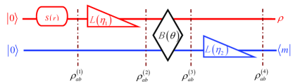
Figure 1: (Colour online) Conceputal scheme of generating MPSSVs.

State in stage 1: The total density operator in this stage can be written as

$$\rho_{ab}^{\left(1\right)}=\left(\rho_{SV}\right)_{a}\otimes\left(\left|0\right\rangle\left\langle 0\right|\right)_{b}$$ (4)

with $\rho_{SV}=S\left(r\right)\left|0\right\rangle\left\langle 0\right|S^{{\dagger}}\left(r\right)$, where the SVS can be further expressed as $S\left(r\right)\left|0\right\rangle=\left(1-\lambda^{2}\right)^{1/4}e^{\frac{\lambda}{2}a^{{\dagger}2}}\left|0\right\rangle$ with $\lambda=\tanh r$. Therefore, $\rho_{ab}^{\left(1\right)}$ can be given by

$$\rho_{ab}^{\left(1\right)}=\int\frac{d^{2}\alpha_{1}d^{2}\beta_{1}}{\pi^{2}}\chi_{\rho_{ab}^{\left(1\right)}}(\alpha_{1},\beta_{1})D_{a}\left(-\alpha_{1}\right)D_{b}\left(-\beta_{1}\right),$$ (5)

where $\chi_{\rho_{ab}^{\left(1\right)}}(\alpha_{1},\beta_{1})$ is the CF of $\rho_{ab}^{\left(1\right)}$ satisfying

$$\chi_{\rho_{ab}^{\left(1\right)}}(\alpha_{1},\beta_{1}) = \mathrm{Tr}[\rho_{ab}^{\left(1\right)}D_{a}\left(\alpha_{1}\right)D_{b}\left(\beta_{1}\right)]$$ (6)

$$= e^{-\allowbreak\frac{(1+\lambda^{2})\left|\alpha_{1}\right|^{2}}{2(1-\lambda^{2})}+\frac{\lambda\allowbreak(\alpha_{1}^{2}+\alpha_{1}^{\ast}{}^{2})}{2(1-\lambda^{2})}-\frac{\left|\beta_{1}\right|^{2}}{2}},$$

and both $D_{a}\left(\alpha_{1}\right)\$and $D_{b}\left(\beta_{1}\right)$ are the displacement operators in mode $a$ and mode $b$, respectively.

State in stage 2: After $\rho_{ab}^{\left(1\right)}$ passing through $L\left(\eta_{1}\right)$, we obtain

$$\rho_{ab}^{\left(2\right)} = \int\frac{d^{2}\alpha_{1}d^{2}\beta_{1}}{\pi^{2}}\chi_{\rho_{ab}^{\left(1\right)}}(\sqrt{1-\eta}\alpha_{1},\beta_{1})$$ (7)

$$\times e^{-\frac{\eta_{1}\left|\alpha_{1}\right|^{2}}{2}}D_{a}\left(-\alpha_{1}\right)D_{b}\left(-\beta_{1}\right).$$

where we have considered the input-output formula in Eq.(2). It is noted that we can still use the CF in stage 1 and it is not necessary to calculate the CF in stage 2.

State in stage 3: Injecting $\rho_{ab}^{\left(2\right)}$ into a variable beam-splitter, we have

$$\rho_{ab}^{\left(3\right)}=B\left(\theta\right)\rho_{ab}^{\left(2\right)}B^{{\dagger}}\left(\theta\right),$$ (8)

where the BS is described by $B\left(\theta\right)=\exp[\theta\left(a^{{\dagger}}b-ab^{{\dagger}}\right)]$ with the transmissivity $T=\cos^{2}\theta$, satisfying $B\left(\theta\right)aB^{{\dagger}}\left(\theta\right)=\sqrt{T}a+\sqrt{1-T}b$ and $B\left(\theta\right)bB^{{\dagger}}\left(\theta\right)=-\sqrt{1-T}a+\sqrt{T}b$ 20 . After making the detailed derivation, $\rho_{ab}^{\left(3\right)}$ can be expressed as

$$\rho_{ab}^{\left(3\right)} = \int\frac{d^{2}\alpha_{1}d^{2}\beta_{1}}{\pi^{2}}\chi_{\rho_{ab}^{\left(1\right)}}(\sqrt{1-\eta_{1}}\alpha_{1},\beta_{1})$$ (9)

$$\times e^{\frac{(1-\eta_{1})\left|\alpha_{1}\right|^{2}}{2}+\frac{\left|\beta_{1}\right|^{2}}{2}}$$

$$\times e^{a(\sqrt{T}\alpha_{1}^{\ast}-\allowbreak\beta_{1}^{\ast}\sqrt{1-T})}e^{-a^{{\dagger}}(\sqrt{T}\alpha_{1}-\beta_{1}\sqrt{1-T})}$$

$$\times e^{b(\alpha_{1}^{\ast}\allowbreak\sqrt{1-T}+\sqrt{T}\beta_{1}^{\ast})}e^{-b^{{\dagger}}(\alpha_{1}\sqrt{1-T}+\sqrt{T}\allowbreak\beta_{1})}.$$

Since the CF of $\rho_{ab}^{\left(3\right)}$ is useful to calculate $\rho_{ab}^{\left(4\right)}$, we must obtain its analytic expression as follows

$$\chi_{\rho_{ab}^{\left(3\right)}}(\alpha_{3},\beta_{3}) = \mathrm{Tr}[\rho_{ab}^{\left(3\right)}D_{a}\left(\alpha_{3}\right)D_{b}\left(\beta_{3}\right)]$$ (10)

$$= e^{-(\frac{1}{2}+\lambda^{2}\tau_{1})\left|\alpha_{3}\right|^{2}+\frac{\lambda\tau_{1}}{2}(\alpha_{3}^{2}+\alpha_{3}^{\ast}{}^{2})}$$

$$\times e^{-(\frac{1}{2}+\lambda^{2}\tau_{2})\left|\beta_{3}\right|^{2}+\allowbreak\frac{1}{2}\lambda\tau_{2}(\beta_{3}^{2}+\beta_{3}^{\ast}{}^{2})}$$

$$\times e^{\lambda\tau_{3}(\alpha_{3}\beta_{3}+\alpha_{3}^{\ast}\beta_{3}^{\ast})-\lambda^{2}\tau_{3}(\alpha_{3}\beta_{3}^{\ast}\allowbreak+\beta_{3}\alpha_{3}^{\ast})},$$

where

$$\tau_{1} = \left(1-\eta_{1}\right)T/\left(1-\lambda^{2}\right),$$

$$\tau_{2} = \left(1-\eta_{1}\right)\left(\allowbreak 1-\allowbreak T\right)/\left(1-\lambda^{2}\right),$$ (11)

$$\tau_{3} = \left(1-\eta_{1}\right)\sqrt{T\left(1-T\right)}/\left(1-\lambda^{2}\right).$$

State in stage 4: After $\rho_{ab}^{\left(3\right)}$ passing through $L\left(\eta_{2}\right)$, similarly using Eq.(2) we also may obtain $\rho_{ab}^{\left(4\right)}$,

$$\rho_{ab}^{\left(4\right)} = \int\frac{d^{2}\alpha_{3}d^{2}\beta_{3}}{\pi^{2}}\chi_{\rho_{ab}^{\left(3\right)}}(\alpha_{3},\sqrt{1-\eta_{2}}\beta_{3})$$ (12)

$$\times e^{-\frac{\eta_{2}\left|\beta_{3}\right|^{2}}{2}}D_{a}\left(-\alpha_{3}\right)D_{b}\left(-\beta_{3}\right).$$

State in stage 5: At the last stage, making a $m$-photon detection, the MPSSV can be obtained

$$\rho=\frac{1}{p_{d}}\left\langle m\right|\rho_{ab}^{\left(4\right)}\left|m\right\rangle,$$ (13)

where $p_{d}$ is the success probability of producing such state. Substituting $\left\langle m\right|=\frac{1}{\sqrt{m!}}\frac{d^{m}}{d\mu^{m}}\left\langle 0\right|e^{\mu b}|_{\mu=0}$ and $\left|m\right\rangle=\frac{1}{\sqrt{m!}}\frac{d^{m}}{d\nu^{m}}e^{\nu b^{{\dagger}}}\left|0\right\rangle|_{\nu=0}$, as well as Eq.(12) into Eq.(13), we obtain the density operator

$$\rho = \frac{1}{m!p_{d}}\frac{d^{2m}}{d\mu^{m}d\nu^{m}}\exp\left(\mu\nu\right)$$ (14)

$$\int\frac{d^{2}\alpha_{3}d^{2}\beta_{3}}{\pi^{2}}\chi_{\rho_{ab}^{\left(3\right)}}(\alpha_{3},\sqrt{1-\eta_{2}}\beta_{3})$$

$$\times e^{-\frac{(1+\eta_{2})\left|\beta_{3}\right|^{2}}{2}-\mu\beta_{3}+\nu\beta_{3}^{\ast}}D_{a}\left(-\alpha_{3}\right)|_{\mu=\nu=0},$$

and its corresponding success probability

$$p_{d}=\frac{1}{m!\sqrt{\epsilon_{4}}}\frac{d^{2m}}{d\mu^{m}d\nu^{m}}e^{(1-\frac{\epsilon_{1}}{\epsilon_{4}})\mu\nu+\frac{\epsilon_{2}}{\epsilon_{4}}\allowbreak(\mu^{2}+\allowbreak\nu^{2})}|_{\mu=\nu=0},$$ (15)

with $\epsilon_{1}=\allowbreak 1+\lambda^{2}\tau_{2}\left(1-\eta_{2}\right)$, $\epsilon_{2}=\frac{1}{2}\lambda\tau_{2}\left(1-\eta_{2}\right)$, and $\epsilon_{4}=\epsilon_{1}^{2}-4\epsilon_{2}^{2}$. Thus, by varying all the interaction parameters, involving the input squeezing parameter $r$, the loss factors $\eta_{1}$, $\eta_{2}$, the BS transmissivity $T$ and the detecting photon number $m$, a broad class of MSSVSs can be obtained.

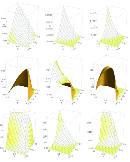
Figure 2: (Colour online) Success probabilities in different paramter space with given other parameters. (Row 1) in ($\eta_{1}$, $\eta_{2}$) space with $r=0.5$, $T=0.97$ and different $m$; (Row 2) in ($r$, $T$) space with $\eta_{1}=\eta_{2}=0.02$; (Row 3) in ($\eta$, $T$) space with $r=0.5$, $\eta_{1}=\eta_{2}=\eta$. Columns 1, Columns 2, and Columns 3 are corresponding to m=1, m=2, and m=3, respectively.

Success probability is an important character in the conditional quantum state engineering. In Fig,2, according to Eq.(15) we plot several distributions of success probability in different parameter spaces. We note that the probability is limited to zero if the loss factors $\eta_{1}$, $\eta_{2}$ equal to 1. Next, we shall discuss the nonclassical properties of the MSSVSs in terms of quadrature squeezing effect, photon number distribution, Wigner function, and explore how the photon subtraction and loss factors affect these nonclassicalities.

III Quadrature squeezing effect

No doubt, the prominent character of the SVS is the quadrature squeezing effect. But compared with the original SVS, how the squeezing effect for the MSSVSs change? Now we explore the quadrature squeezing effect of the MSSVSs.

The coordinate operator is defined as $X=\left(a+a^{{\dagger}}\right)/\sqrt{2}$ and the momentum operator is defined as $P=\left(a-a^{{\dagger}}\right)/(\sqrt{2}i)$. Their respective variances can expressed as follows 21-1 ; 21-2

$$\Delta^{2}X = \left\langle a^{{\dagger}}a\right\rangle-\left|\left\langle a^{{\dagger}}\right\rangle\right|^{2}+\text{Re}(\left\langle a^{{\dagger}2}\right\rangle-\left\langle a^{{\dagger}}\right\rangle^{2})+\frac{1}{2},$$

$$\Delta^{2}P = \left\langle a^{{\dagger}}a\right\rangle-\left|\left\langle a^{{\dagger}}\right\rangle\right|^{2}-\text{Re}(\left\langle a^{{\dagger}2}\right\rangle-\left\langle a^{{\dagger}}\right\rangle^{2})+\frac{1}{2}.$$ (16)

Their uncertainty relation obeys $\Delta^{2}X\Delta^{2}P\geq 1/4$. In particular, a coherent (or vacuum) state holds $\Delta^{2}X=\Delta^{2}P=1/2$. Generally, a quantum state is called squeezing if $\Delta^{2}X<1/2$ or $\Delta^{2}P$ $<1/2$.

In order to study the squeezing effect, one can firstly calculate the general expected value $\left\langle a^{{\dagger}k}a^{l}\right\rangle=\mathrm{Tr}\left(a^{{\dagger}k}a^{l}\rho\right)$ with different integers $k,l$ for quantum state $\rho$. By choosing proper integers $k,l$, one can obtain any expected values one needed. In the process of calculation, one can resort to the techniques $a^{{\dagger}k}=\frac{d^{k}}{df^{k}}e^{fa^{{\dagger}}}|_{f=0}$ and $a^{l}=\frac{d^{l}}{dg^{l}}e^{ga}|_{g=0}$.

For example, the SVS has

$$\left\langle a^{{\dagger}k}a^{l}\right\rangle_{\rho_{SV}}=\frac{d^{k+l}}{df^{k}dg^{l}}e^{\frac{1}{1-\lambda^{2}}\frac{\lambda}{2}\left(f^{2}+g^{2}\right)+\frac{\lambda^{2}}{1-\lambda^{2}}fg}|_{f=g=0}.$$ (17)

When $k=l=1$, it leads to $\left\langle a^{{\dagger}}a\right\rangle_{\rho_{SV}}=\lambda^{2}/\left(1-\lambda^{2}\right)$. If $k=1,l=0$ and $k=2,l=0$, we have $\left\langle a^{{\dagger}}\right\rangle=0$ and $\left\langle a^{{\dagger}2}\right\rangle=\lambda/\left(1-\lambda^{2}\right),$ respectively. Thus for the SVS $\rho_{SV}$, $\Delta^{2}X=\frac{1}{2}e^{2r}$ and $\Delta^{2}P=\frac{1}{2}e^{-2r}$. So the SVS has squeezing effect for any nonzero $r$. While for the MSSVSs, we have

$$\left\langle a^{{\dagger}k}a^{l}\right\rangle = \frac{1}{m!p_{d}\sqrt{\epsilon_{4}}}\frac{d^{2m+k+l}}{d\mu^{m}d\nu^{m}df^{k}dg^{l}}$$ (18)

$$e^{\frac{\epsilon_{3}\epsilon_{7}}{\epsilon_{4}}\left(\mu f+\allowbreak g\nu\right)+\allowbreak\frac{\epsilon_{3}\epsilon_{8}}{\epsilon_{4}}\left(\nu f+g\allowbreak\mu\right)}$$

$$\times e^{(\lambda^{2}\tau_{1}+\frac{\epsilon_{5}}{\epsilon_{4}})fg+(\frac{1}{2}\lambda\tau_{1}+\frac{\epsilon_{6}}{\epsilon_{4}})\left(f^{2}+g^{2}\right)}$$

$$\times e^{(1-\frac{\epsilon_{1}}{\epsilon_{4}})\mu\nu+\frac{\epsilon_{2}}{\epsilon_{4}}\left(\mu^{2}+\nu^{2}\right)}|_{f=g=\mu=\nu=0}$$

with $\epsilon_{3}=\lambda\tau_{3}\sqrt{1-\eta_{2}}$, $\epsilon_{5}=4\lambda\epsilon_{2}\epsilon_{3}^{2}-\left(1+\lambda^{2}\right)\epsilon_{1}\epsilon_{3}^{2}$, $\epsilon_{6}=\left(1+\allowbreak\lambda^{2}\right)\epsilon_{2}\epsilon_{3}^{2}-\lambda\epsilon_{1}\epsilon_{3}^{2}$, $\epsilon_{7}=\lambda\epsilon_{1}-2\epsilon_{2}$, and $\epsilon_{8}=\epsilon_{1}-2\lambda\epsilon_{2}$.

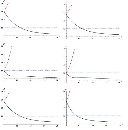
Figure 3: (Colour online) Quadrature squeezing effect vesus $r$ for the MPSSV with fixed $T=0.9$ and (row 1) $m=1$, (row 2) $m=2$, (row 3) $m=3$ and (left column) $\eta_{1}=\eta_{1}=0$, (right column) $\eta_{1}=\eta_{1}=0.1$. Notice that the black solid line, the red dashed line, and the blue dotdashed line are corresponding to $\Delta^{2}P$, $\Delta^{2}X$ and $1/2$, respectively. Notice the threshold value is different in each sub-figure.

In Fig.3, we plot the variation of $\Delta^{2}P$ and $\Delta^{2}X$ versus $r$ for several different cases at fixed $T=0.9$. It is clearly seen that the variance of $\Delta^{2}P$ monotonously decreases as $r$ increases for a given $m$ and there exists squeezing in $P$ quadrature component within a certain range of parameter $r$. For the case of $m=1$, only when the squeezing parameter $r$ is bigger than a threshold value $r_{c}$, depending on the loss factor, the MSSVS may have the possibility of the squeezing effect (Noticing $r_{c}=0.626381$ for $\eta_{1}=\eta_{2}=0$ and $r_{c}=0.609918$ for $\eta_{1}=\eta_{2}=0.1$). For the case of $m=2$, the MSSVS always presents the squeezing effect for any nonzero $r$. For the case of $m=3$, only when the squeezing parameter $r$ is bigger than a threshold value $r_{c}$, the MSSVS may have the possibility of the squeezing effect, where $r_{c}=0.396049$ for $\eta_{1}=\eta_{2}=0$ and $r_{c}=0.387008$ for $\eta_{1}=\eta_{2}=0.1$, respectively.

IV Photon number distribution

Photon number distribution (PND) is defined by $P\left(n\right)=\left\langle n\right|\rho\left|n\right\rangle$, which means the probability of detecting $n$ photons in the field $\rho$. Using the technique $\left\langle n\right|=\frac{1}{\sqrt{n!}}\frac{d^{n}}{ds^{n}}\left\langle 0\right|e^{sa}|_{s=0}$ and $\left|n\right\rangle=\frac{1}{\sqrt{n!}}\frac{d^{n}}{dt^{n}}e^{ta^{{\dagger}}}\left|0\right\rangle|_{t=0}$, one can easily obtain the PNDs for the given optical field $\rho$.

For the SVS $\rho_{SV}$, we have

$$P_{\rho_{SV}}\left(n\right) = \frac{\left(1-\lambda^{2}\right)^{1/2}}{n!}\frac{d^{2n}}{ds^{n}dt^{n}}e^{\frac{\lambda}{2}(s^{2}+t^{2})}|_{s=t=0}$$ (21)

$$= \left\{\begin{array}[]{cc}\frac{n!\lambda^{n}\left(1-\lambda^{2}\right)^{1/2}}{2^{n}\left(\frac{n}{2}\right)!\left(\frac{n}{2}\right)!},&n\text{ is even,}\\ 0,&n\text{ is odd,}\end{array}\right.$$

which implies that the SVS contains only even-photon components, as seen from Fig.4. This is one of the key characteristics of the SVS.

But what will happen to the PNDs for the MSSVSs? Noticing Eq.(14), we obtain the PND of the MSSVSs expressed as

$$P\left(n\right) = \frac{1}{n!m!p_{d}\sqrt{\epsilon_{4}\kappa_{4}}}\frac{d^{2m+2n}}{d\mu^{m}d\nu^{m}ds^{n}dt^{n}}$$ (22)

$$e^{[1-\frac{\epsilon_{1}}{\epsilon_{4}}+\frac{\kappa_{3}^{2}}{\kappa_{4}}\left(\kappa_{1}\kappa_{5}+4\kappa_{2}\kappa_{6}\right)]\mu\nu+(1-\frac{\kappa_{1}}{\kappa_{4}})st}$$

$$\times e^{[\frac{\epsilon_{2}}{\epsilon_{4}}-\frac{\kappa_{3}^{2}}{\kappa_{4}}\left(\kappa_{1}\kappa_{6}+\kappa_{2}\kappa_{5}\right)]\left(\mu^{2}+\allowbreak\nu^{2}\right)+\frac{\kappa_{2}}{\kappa_{4}}\left(s^{2}+\allowbreak t^{2}\right)}$$

$$\times e^{\frac{\kappa_{3}}{\kappa_{4}}[\kappa_{7}\left(\mu t+s\nu\right)+\kappa_{8}\left(\mu s+\nu t\right)]}|_{\mu=\nu=s=t=0},$$

where $\kappa_{1}=1+\lambda^{2}\tau_{1}+\frac{\allowbreak\epsilon_{5}}{\epsilon_{4}}$, $\kappa_{2}=\frac{1}{2}\lambda\tau_{1}+\frac{\epsilon_{6}}{\epsilon_{4}}$, $\kappa_{3}=\frac{\epsilon_{3}}{\epsilon_{4}}$, $\kappa_{4}=\kappa_{1}^{2}-4\kappa_{2}^{2}$, $\kappa_{5}=8\lambda\epsilon_{1}\epsilon_{2}-\left(1+\allowbreak\lambda^{2}\right)\left(\epsilon_{1}^{2}+\allowbreak 4\epsilon_{2}^{2}\right)$, $\kappa_{6}=\lambda\left(\epsilon_{1}^{2}+4\epsilon_{2}^{2}\right)-2\left(1+\lambda^{2}\right)\epsilon_{1}\epsilon_{2}$, $\kappa_{7}=\kappa_{1}\epsilon_{7}-2\kappa_{2}\epsilon_{8}$, and $\kappa_{8}=\kappa_{1}\epsilon_{8}-2\kappa_{2}\epsilon_{7}$.

In order to analyze the effect of loss on the PNDs of the MPSSVs, we depict the PNDs in Fig.5 and Fig.6. From Fig.5 without loss ($\eta_{1}=0$, $\eta_{2}=0$), we see that the MPSSVs contain only even-photon (odd-photon) components if $m$ is even (odd), which agrees with the results of Ref.9-1 . However, we observe that, surprisingly, if there is the loss, the MPSSVs contain all-photon components (see Fig.6). Moreover, the ratio between even-component and odd-component can be adjusted by the value of $m$ and the loss factors $\eta_{1}$, $\eta_{2}$.

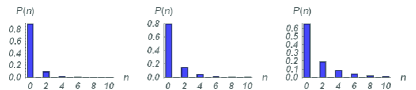
Figure 4: (Colour online) PNDs for the SVs with $r=0.5$, $0.7$, $1$, respectively.

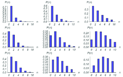
Figure 5: (Colour online) PNDs for the MPSSVs wihtout loss ($\eta_{1}=0$, $\eta_{2}=0$) with given other parameters. (Row 1) with $T=0.9$, $m=1$; (Row 2) with $T=0.9$, $m=2$; (Row 3) with $T=0.9$, $m=3$. Column 1, column 2, and column 3 are corresponding to $r=0.5$, $r=0.7$, and $r=1$, respectively.

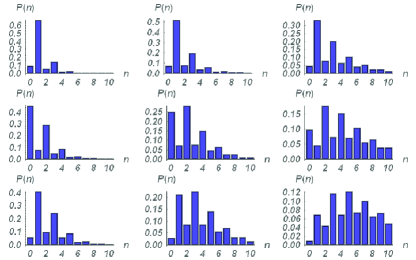
Figure 6: (Colour online) PNDs for the MPSSVs wiht loss ($\eta_{1}=0.1$, $\eta_{2}=0.1$) with given other parameters. (Row 1) with $T=0.9$, $m=1$ and different $r$; (Row 2) with $T=0.9$, $m=2$ and different $r$; (Row 3) with $T=0.9$, $m=3$ and different $r$. Column 1, column 2, and column 3 are corresponding to $r=0.5$, $r=0.7$, and $r=1$, respectively.

V Wigner function

Wigner function $W\left(\beta\right)$ for quantum state $\rho$ can be defined by22

$$W\left(\beta\right)=\frac{2}{\pi}\mathrm{Tr}[\rho D\left(\beta\right)\left(-1\right)^{a^{{\dagger}}a}D^{{\dagger}}\left(\beta\right)],$$ (23)

where $D\left(\beta\right)=\exp\left(\beta a^{{\dagger}}-\beta^{\ast}a\right)$ is the usual displacement operator with $\beta=\left(x+iy\right)/\sqrt{2}$.

For the SVS, we know

$$W_{\rho_{SV}}\left(\beta\right)=\frac{2}{\pi}e^{-\frac{2(1+\lambda^{2})}{1-\lambda^{2}}\left|\beta\right|^{2}+\allowbreak\frac{2\lambda}{1-\lambda^{2}}\left(\beta^{2}+\beta^{\ast}{}^{2}\allowbreak\right)},$$ (24)

which is Gaussian and implies that the SVS are Gaussian states (see Fig.7). While for the MSSVSs , we have

$$W\left(\beta\right) = \frac{1}{\pi m!p_{d}\sqrt{\epsilon_{4}\kappa_{9}}}e^{-(\frac{\kappa_{1}}{\kappa_{9}}-\frac{1}{2\kappa_{9}})\left|\beta\right|^{2}+\frac{\kappa_{2}}{\kappa_{9}}\left(\beta^{2}+\allowbreak\beta^{\ast}{}^{2}\right)}$$ (25)

$$\frac{d^{2m}}{d\mu^{m}d\nu^{m}}e^{[1-\frac{\epsilon_{1}}{\epsilon_{4}}+\frac{\kappa_{3}^{2}}{\kappa_{9}}(4\kappa_{2}\kappa_{6}+\kappa_{1}\kappa_{5}-\frac{1}{2}\kappa_{5})]\mu\nu}$$

$$\times e^{[\frac{\epsilon_{2}}{\epsilon_{4}}+\frac{\kappa_{3}^{2}}{\kappa_{9}}(\frac{1}{2}\kappa_{6}-\kappa_{1}\kappa_{6}-\kappa_{2}\kappa_{5})]\left(\mu^{2}+\nu^{2}\right)}$$

$$\times e^{[(\frac{\kappa_{1}}{\kappa_{9}}-\frac{1}{2\kappa_{9}})\kappa_{3}\epsilon_{8}-\frac{\allowbreak 2\kappa_{2}}{\kappa_{9}}\kappa_{3}\epsilon_{7}]\left(\nu\beta+\mu\beta^{\ast}\right)}$$

$$\times e^{[(\frac{\kappa_{1}}{\kappa_{9}}-\frac{1}{2\kappa_{9}})\kappa_{3}\epsilon_{7}-\frac{\allowbreak 2\kappa_{2}}{\kappa_{9}}\kappa_{3}\epsilon_{8}]\left(\mu\beta+\nu\beta^{\ast}\right)}|_{\mu=\nu=0},$$

where $\kappa_{9}=(\kappa_{1}-\frac{1}{2})^{2}-4\kappa_{2}^{2}$.

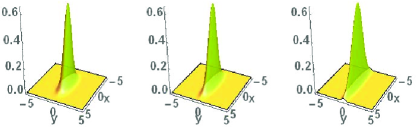
Figure 7: (Colour online) Wigner functions for the SVs with $r=0.5$, $0.7$, $1$, respectively.

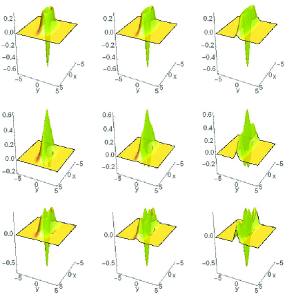
Figure 8: (Colour online) Wigner functions for the MPSSV without loss ($\eta_{1}=0$, $\eta_{2}=0$) with given other parameters. (Row 1) with $T=0.9$, $m=1$; (Row 2) with $T=0.9$, $m=2$; (Row 3) with $T=0.9$, $m=3$. Column 1, Column 2, and Column 3 are corresponding to $r=0.5$, $r=0.7$, and $r=1$, respectively.

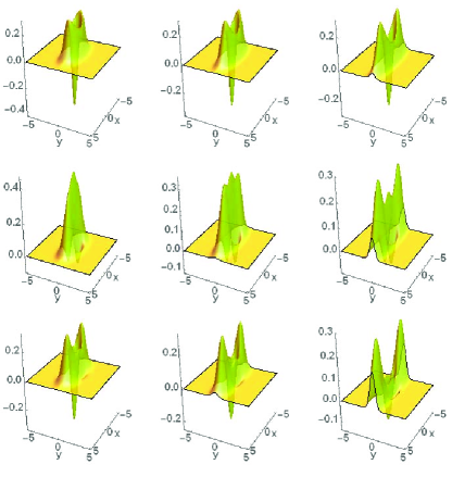
Figure 9: (Colour online) Wigner functions for the MPSSV without loss ($\eta_{1}=0.1$, $\eta_{2}=0.1$) with given other parameters. (Row 1) with $T=0.9$, $m=1$; (Row 2) with $T=0.9$, $m=2$; (Row 3) with $T=0.9$, $m=3$. Column 1, Column 2, and Column 3 are corresponding to $r=0.5$, $r=0.7$, and $r=1$, respectively.

According to Eq.(25), we plot the Wigner functions of the MSSVSs in Fig.8 without loss and in Fig.9 with loss in phase space. Clearly, the Wigner functions of the MSSVSs is non-Gaussian in phase space. The surfaces without loss in Fig.8 are smoother than those with loss in Fig.9. As an evidence of the nonclassicality of the state23 , there are some negative regions of the Wigner function in phase space (see Figs. 8 and 9). Moreover, the distribution of Wigner function can reflect the non-Gaussianity of quantum states24 ; 25 .

VI Conclusion

To summarize, we present a conditional scheme of generating the MSSVSs in the presence of pure-loss channels. By adjusting the relative interaction parameters (including $r$, $\eta_{1}$, $\eta_{2}$, $T$ and $m$), a broad class of MSSVSs with figure of merit can be obtained. For the theoretical model, we have given the complete description of density operator of the optical fields in terms of CF. Analytical derivation and numerical simulation for the properties of the MSSVSs are explored in detail. Compared with the original SVS and the MSSVSs without loss, some interesting results effected by the loss are summarized as follows: (1) The losses change a threshold value of original squeezing parameter, which may present the appearance of squeezing effect; (2) The losses will let the MSSVSs contain all-photon components (including odd-photon and even-photon); (3) The losses make the distribution of the Wigner function more complex.

References

(1) S. L. Braunstein and P. van Loock, Quantum information with
continuous variables, Rev. Mod. Phys. 77, 513-577 (2005).
(2) A. Serafini, Quantum continuous variables, A primer of
theoretical methods, CRC Press, Taylor & Francis Group (2017).
(3) X. B. Wang, T. Hiroshima, A. Tomita, M. Hayashi, Quantum
information with Gaussian states, 448, 1-111 (2007).
(4) C. N. Gagatsos and S. Guha, Efficient representation of Gaussian
states for multimode non-Gaussian quantum state engineering via subtraction
of arbitrary number of photons, Phys. Rev. A 99, 053816 (2019).
(5) S. Lloyd and S. L. Braunstein, Quantum computation over
continuous variables, Phys. Rev. Lett. 82, 1784-1787 (1999).
(6) J. P. Dowling, Quantum optical metrology - the lowdown on
high-N00N states, Contemporary Physics 49, 125-143 (2008).
(7) C. Navarrete-Benlloch, R. Garcia-Patron, J. H. Shapiro, and N.
J. Cerf, Enhancing quantum entanglement by photon addition and subtraction,
Phys. Rev. A 86, 012328 (2012).
(8) T. J. Bartley, P. J. D. Crowley, A. Datta, J. Nunn, L. Zhang,
and I. Walmsley, Strategies for enhancing quantum entanglement by local
photon subtraction, Phys. Rev. A 87, 022313 (2013).
(9) T. Opatrny, G. Kurizki, and D. G. Welsch, Improvement on
teleportation of continuous variables by photon subtraction via conditional
measurement, Phys. Rev. A 61, 032302 (2000).
(10) A. Biswas and G. S. Agarwal, Nonclassicality and decoherence
of photon-subtracted squeezed states, Phys. Rev. A 75, 032104 (2007).
(11) A. Ourjoumtsev, R. Tualle-Brouri, J. Laurat, P. Grangier,
Generating Optical Schrodinger Kittens for Quantum Information Processing,
Science, 312, 83-86 (2006).
(12) T. Gerrits, S. Glancy, T. S. Clement, B. Calkins, A. E. Lita,
A. J. Miller, A. L. Migdall, S. W. Nam, R. P. Mirin, and E. Knill,
Generation of optical coherent-state superpositions by number-resolved
photon subtraction from the squeezed vacuum, Phys. Rev. A 82, 031802(R)
(2010).
(13) M. Dakna, T. Anhut, T. Opatrny, L. Knoll, and D. G. Welsch,
Generating Schrodinger-cat-like states by means of conditional measurements
on a beam splitter, Phys. Rev. A 55, 3184-3194 (1997).
(14) A. E. Ulanov, I. A. Fedorov, A. A. Pushkina, Y. V. Kurochkin,
T. C. Ralph and A. I. Lvovsky, Undoing the effect of loss on quantum
entanglement, Nature Photonics, 9, 764-768 (2015).
(15) B. Hacker, S. Wette, S. Daiss, A. Shaukat, S. Ritter, L. Li,
and G. Rempe, Deterministic creation of entangled atom–light
Schrodinger-cat states, Nature Photonics, 13, 110–115 (2019).
(16) N. Quesada, L. G. Helt, J. Izaac, J. M. Arrazola, R.
Shahrokhshahi, C. R. Myers, and K. K. Sabapathy, Simulating realistic
non-Gaussian state preparation, Phys. Rev. A 100, 022341 (2019).
(17) F. Dell’Anno, S. De Siena, and F. Illuminati, Realistic
continuous-variable quantum teleportation with non-Gaussian resources, Phys.
Rev. A 81, 012333 (2010).
(18) K. E. Cahill and R. J. Glauber, Density operators and
quasiprobability distributions, Phys. Rev. 177, 1882-1902 (1969).
(19) P. Marian and T. A. Marian, Continuous-variable teleportation
in the characteristic-function description, Phys. Rev. A 74, 042306 (2006).
(20) X. X. Xu and H. C. Yuan, Some evolution formulas on the optical
fields propagation in realistic environments, Int. J. Theor. Phys. 56,
791-801 (2017).
(21) M. O. Scully and M. S. Zubairy, Quantum optics (Cambridge
University Press, 1997).
(22) S. M. Barnett and P. M. Radmore, Methods in theoretical quantum
optics (Clarendon Press, Oxford, 1997).
(23) R. Loudon, The quantum theory of light, Oxford University
Press, New York, 2000.
(24) P. Malpani, N. Alam, K. Thapliyal, A. Pathak, V. Narayanan,
and S. Banerijee, Ann. Phys. (Berlin) 531 1800318 (2019).
(25) G. Auletta, Foundations and interpretation of quantum
mechanics, World Scientific, Singapore, 2001.
(26) A. Kenfack and K. Zyczkowski, Negativity of theWigner function
as an indicator of non-classicality, J. Opt. B: Quantum Semiclass. Opt. 6,
396-404 (2004).
(27) F. Albarelli, M. G. Genoni, M. G. A. Paris, and A. Ferraro,
Resource theory of quantum non-Gaussianity andWigner negativity, Phys. Rev.
A 98, 052350 (2018).
(28) R. Takagi and Q. Zhuang, Convex resource theory of
non-Gaussianity, Phys. Rev. A 97, 062337 (2018).