PQ-NET: A Generative Part Seq2Seq Network for 3D Shapes

Abstract

We introduce PQ-NET, a deep neural network which represents and generates 3D shapes via sequential part assembly. The input to our network is a 3D shape segmented into parts, where each part is first encoded into a feature representation using a part autoencoder. The core component of PQ-NET is a sequence-to-sequence or Seq2Seq autoencoder which encodes a sequence of part features into a latent vector of fixed size, and the decoder reconstructs the 3D shape, one part at a time, resulting in a sequential assembly. The latent space formed by the Seq2Seq encoder encodes both part structure and fine part geometry. The decoder can be adapted to perform several generative tasks including shape autoencoding, interpolation, novel shape generation, and single-view 3D reconstruction, where the generated shapes are all composed of meaningful parts.

“The characterization of object perception provided by recognition-by-components (RBC) bears a close resemblance to some current views as to how speech is perceived.”

— Irving Biederman [5]

1 Introduction

Learning generative models of 3D shapes is a key problem in both computer vision and computer graphics. While graphics is mainly concerned with 3D shape modeling, in inverse graphics [23], a major line of work in computer vision, one aims to infer, often from a single image, a disentangled representation with respect to 3D shape and scene structures [29]. Lately, there has been a steady stream of works on developing deep neural networks for 3D shape generation using different shape representations, e.g., voxel grids [54], point clouds [15, 1], meshes [20, 51], and most recently, implicit functions [35, 41, 10, 56]. However, most of these works produce unstructured 3D shapes, despite the fact that object perception is generally believed to be a process of structural understanding, i.e., to infer shape parts, their compositions, and inter-part relations [24, 5].

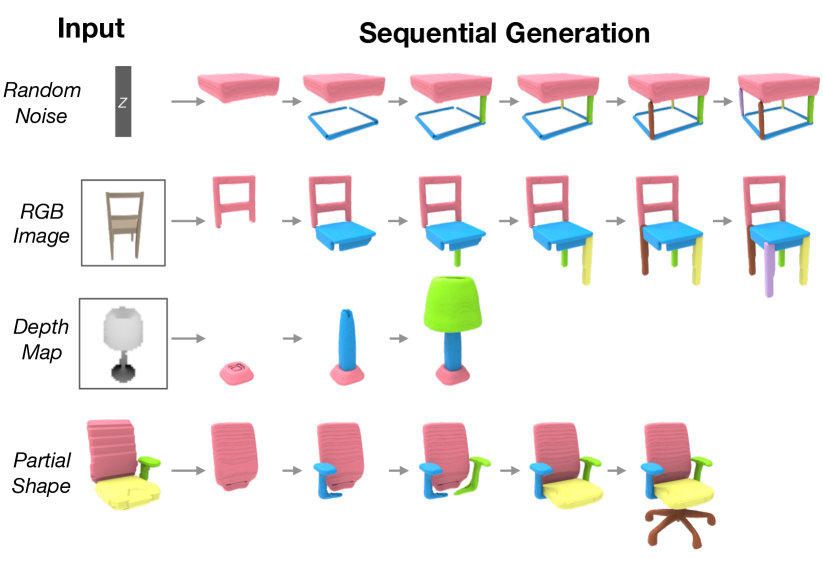
Figure 1: Our network, PQ-NET, learns 3D shape representations as a sequential part assembly. It can be adapted to generative tasks such as random 3D shape generation, single-view 3D reconstruction (from RGB or depth images), and shape completion.

In this paper, we introduce a deep neural network which represents and generates 3D shapes via sequential part assembly, as shown in Figures 1 and 2. In a way, we regard the assembly sequence as a “sentence” which organizes and describes the parts constituting a 3D shape. Our approach is inspired, in part, by the resemblance between speech and shape perception, as suggested by the seminal work of Biederman [5] on recognition-by-components (RBC). Another related observation is that the phase structure rules for language parsing, first introduced by Noam Chomsky, take on the view that a sentence is both a linear string of words and a hierarchical structure with phrases nested in phrases [7]. In the context of shape structure presentations, our network adheres to linear part orders, while other works [53, 31, 36] have opted for hierarchical part organizations.

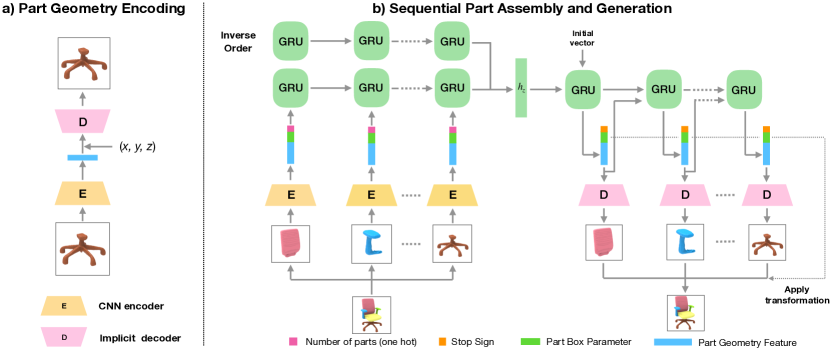
Figure 2: The architecture of PQ-NET: our part Seq2Seq generative network for 3D shapes.

The input to our network is a 3D shape segmented into parts, where each part is first encoded into a feature representation using a part autoencoder; see Figure 2(a). The core component of our network is a sequence-to-sequence or Seq2Seq autoencoder which encodes a sequence of part features into a latent vector of fixed size, and the decoder reconstructs the 3D shape, one part at a time, resulting in a sequential assembly; see Figure 2(b). With its part-wise Seq2Seq architecture, our network is coined PQ-NET. The latent space formed by the Seq2Seq encoder enables us to adapt the decoder to perform several generative tasks including shape autoencoding, interpolation, new shape generation, and single-view 3D reconstruction, where all the generated shapes are composed of meaningful parts.

As training data, we take the segmented 3D shapes from PartNet [37], which is built on ShapeNet [8]. The shape parts are always specified in a file following some linear order in the dataset; our network takes the part order that is in a shape file. We train the part and Seq2Seq autoencoders of PQ-NET separately, either per shape category or across all categories of PartNet.

Our part autoencoder adapts IM-NET [10] to encode shape parts, rather than whole shapes, with the decoder producing an implicit field. The part Seq2Seq autoencoder follows a similar architecture as the original Seq2Seq network developed for machine translation [47]. Specifically, the encoder is a bidirectional stacked recurrent neural network (RNN) [45] that inputs two sequences of part features, in opposite orders, and outputs a latent vector. The decoder is also a stacked RNN, which decodes the latent vector representing the whole shape into a sequential part assembly.

PQ-NET is the first fully generative network which learns a 3D shape representation in the form of sequential part assembly. The only prior part sequence model was 3D-PRNN [58], which generates part boxes, not their geometry — our network jointly encodes and decodes part structure and geometry. PQ-NET can be easily adapted to various generative tasks including shape autoencoding, novel shape generation, structured single-view 3D reconstruction from both RGB and depth images, and shape completion. Through extensive experiments, we demonstrate that the performance and output quality of our network is comparable or superior to state-of-the-art generative models including 3D-PRNN [58], IM-NET [10], and StructureNet [36].

2 Related work

Structural analysis of 3D shapes.

Studies on 3D shape variabilities date back to statistical modeling of human faces [6] and bodies [2], e.g., using PCA. Learning structural variations of man-made shapes is a more difficult task. Earlier works from graphics typically infer one or more parametric templates of part arrangement from shape collections [40, 27, 17]. These methods often require part correspondence of the input shapes. Probabilistic graphical models can be used to model shape variability as the causal relations between shape parts [26], but pre-segmented and part labeled shapes are required for learning such models.

“Holistic” generative models of 3D shapes.

Deep generative models of 3D shapes have been developed for volumetric grids [54, 19, 52, 43], point clouds [15, 1, 57], surface meshes [20, 51], multi-view images [46], and implicit functions [11, 41]. Common to these works is that the shape variability is modeled in a holistic, structure-oblivious fashion. This is mainly because there are few part-based shape representations suitable for deep learning.

Part-based generative models.

In recent years, learning deep generative models for part- or structure-aware shape synthesis has been gaining more interests. Huang et al. [25] propose a deep generative model based on part-based templates learned a priori. Nash and Williams [38] propose a ShapeVAE to generate segmented 3D objects and the model is trained using shapes with dense point correspondence. Li et al. [31] propose GRASS, an end-to-end deep generative model of part structures. They employ recursive neural network (RvNN) to attain hierarchical encoding and decoding of parts and relations. Their binary-tree-based RvNN is later extended to the N-ary case by StructureNet [36]. Wu et al. [55] couple the synthesis of intra-part geometry and inter-part structure. In G2L [50], 3D shapes are generated with part labeling based on generative adversarial networks (GANs) and then refined using a pre-trained part refiner. Most recently, Gao et al. [18] train an autoencoder to generate a spatial arrangement of closed, deformable mesh parts respecting the global part structure of a shape category.

Other recent works on part-based generation adopts a generate-and-assemble scheme. CompoNet [44] is a part composition network operating on a fixed number of parts. Per-part generators and a composition network are trained to produce shapes with a given part structure. Dubrovina et al. [14] propose a decomposer-composer network to learn a factorized shape embedding space for part-based modeling. Novel shapes are synthesized by randomly sampling and assembling the pre-exiting parts embedded in the factorized latent space. Li et al. [30] propose PAGENet which is composed of an array of per-part VAE-GANs, followed by a part assembly module that estimates a transformation for each part to assemble them into a plausible structure.

Seq2Seq.

Seq2Seq is a general-purpose encoder-decoder framework for machine translation. It is composed of two RNNs which takes as input a word sequence and maps it into an output one with a tag and attention value [47]. To date, Seq2Seq has been used for a variety of different applications such as image captioning, conversational models, text summarization, as well as few works for 3D representation learning. For example, Liu et al. [32] employ Seq2Seq to learn features for 3D point clouds with multi-scale context. PQ-NET is the first deep neural network that exploits the power of sequence-to-sequence translation for generative 3D shape modeling, by learning structural context within a sequence of constituent shape parts.

3D-PRNN: part sequence assembly.

Most closely related to our work is 3D-PRNN [58], which, to the best of our knowledge, is the only prior work that learns a part sequence model for 3D shapes. Specifically, 3D-PRNN is trained to reconstruct 3D shapes as sequences of box primitives given a single depth image. In contrast, our network learns a deep generative model of both a linear arrangement of shape parts and geometries of the individual parts. Technically, while both networks employ RNNs, PQ-NET learns a shape latent space, jointly encoding both structure and geometry, using a Seq2Seq approach. 3D-PRNN, on the other hand, uses the RNN as a recurrent generator that sequentially outputs box primitives based on the depth input and the previously generated single primitive. Their network is trained on segmented shapes whose parts are ordered along the vertical direction. To allow novel shape generation, 3D-PRNN needs to be initiated by primitive parameters sampled from the training set, while PQ-NET follows a standard generative procedure using latent GANs [1, 10].

Single view 3D reconstruction (SVR).

Most methods train convolutional networks that map 2D images to 3D shapes using direct 3D supervision, where voxel [13, 19, 48, 42, 28] and point cloud [16, 34] representations of 3D shapes have been extensively utilized. Some methods [33, 4] learn to produce multi-view depth maps that are fused together into a 3D point cloud. Tulsiani et al. [49] infer cuboid abstraction of 3D shapes from single-view images. Extending the RvNN-based architecture of GRASS [31], Niu et al. [39] propose Im2Struct which maps a single-view image into a hierarchy of part boxes. Differently from this work, our method produces part boxes and the corresponding part geometries jointly, by exploiting the coupling between structure and geometry in a sequential part generative model.

3 Method

In this section, we introduce our PQ-NET, based on a Seq2Seq Autoencoder, or Seq2SeqAE, for sequential part assembly and part-based shape representation. Given a 3D shape consisting of several parts, we first represents it as a sequence with each vector corresponding to a single part that consists of a geometric feature vector and a 6 DoF bounding box indicating the translating and scaling of part local frame according to the global coordinate system. The geometry of each part is projected to a low-dimensional feature space based on a hybrid-structure autoencoder using self-supervised training. Since the number of part sequence is un-known, we seek a recurrent neural network based encoder to transform the entire sequence to an unified shape latent space. The part sequence is then decoded from the shape feature vector, with each part containing the geometry feature and the spatial position and size. Figure 2 shows the outline of our Seq2SeqAE model. Our learned shape latent space facilitates applications like random generation, single view reconstruction and shape completion, etc. We will explain the two major components of our model in the next sections with more details in supplementary material.

3.1 Part Geometry Auto-encoding

The part geometry and topology is much simpler than the original shape. Thus, by decomposing the shape into a set of parts, we are able to perform high-resolution and cross-category geometry learning with high quality. Our part geometry autoencoder uses a similar design as  [10], where a CNN-based encoder projects voxelized part to the part latent space, and a MLP-based decoder re-projects the latent vector to a volumetric Signed Distance Field(SDF). The surface of the object is retrieved using marching cube on the places where SDF is zero.

We first scale each part to a fixed resolution $64\times 64\times 64$ within its bounding box and feed scaled part volume as input to a CNN encoder to get the output feature vector $g$ that represents the part geometry. The MLP decoder takes in this feature vector $g$ and 3D point $(x,y,z)$ and output a single value that tells either this point is inside the surface of the input geometry or outside. Since volumetric SDF is continuous everywhere, the output geometry is smooth and can be sampled at any resolution. Note that this feature representation has no information about the part’s scale and global position, and thus purely captures its geometry property. For a shape with $n$ parts, we can extract a sequence of geometry features $g_{1},g_{2},...,g_{n}$ corresponding to each part.

3.2 Seq2Seq AE

The core of our neural network is a Sequence-to-Sequence(Seq2Seq) Autoencoder. The sequential encoder is a bidirectional stacked RNN [45] that takes a sequence of part features, along with its reverse version, as the input, and outputs a latent vector $h_{z}$ of fixed size. This latent vector is then passed to the stacked RNN decoder that outputs a part feature at each time step. Intuitively, the Seq2Seq encoder learns to assemble parts into a complete shape while the decoder learns to decompose it into meaningful parts. In all of our experiments, we used GRU [12] as the RNN cell and employed two hidden layers for each RNN.

More specifically, let $F_{i}=[g_{i};b_{i}]$ denotes part feature vector, concatenated with two components, a part geometry feature $g_{i}$ and a 6 DoF bounding box $b_{i}=[x_{i},y_{i},z_{i},l_{i},m_{i},n_{i}]$, where $[x_{i},y_{i},z_{i}]$ and $[l_{i},m_{i},n_{i}]$ indicate box position and size, respectively. An additional information of part number is used to regularize the shape distribution, since we empirically found it improving the performance. With the extra one-hot vector $t_{i}$ of part number, the full vector of a part is finally symbolized as $S_{i}=[F_{i};t_{i}]$. We feed the sequence of $S=[S_{1},S_{2},...,S_{n}]$ and also its reverse, $S_{reverse}$, to the bidirectional encoder, and obtain two hidden states from the output,

$$\begin{split}h_{1}=[h_{1}^{1};h_{1}^{2}]&=\mathrm{encode_{1}}(S)\\ h_{2}=[h_{2}^{1};h_{2}^{2}]&=\mathrm{encode_{2}}(S_{reverse})\\ h_{z}&=[h_{1}^{1};h_{2}^{1};h_{1}^{2};h_{2}^{2}]\end{split}$$ (1)

The final state $h_{z}$ is a latent representation of 3D shape.

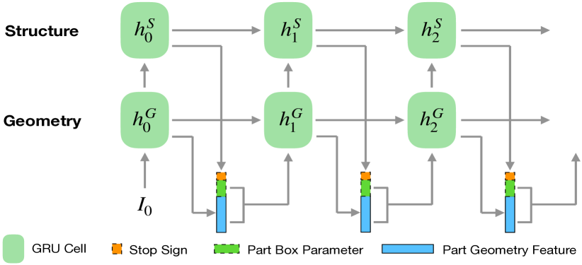
Figure 3: Structure of our stacked RNN decoder. At each time step, the geometry feature and structure feature are separately predicted, along with a stop sign indicating whether the iteration is finished.

Different to the vanilla RNN, stacked RNN outputs more than one vector for each time step, which allows more complex representation for our parts. Specifically, our stacked RNN has two hidden states at each time step, namely $h_{i}^{G}$ and $h_{i}^{S}$. We use $h_{i}^{G}$ for geometry feature reconstruction by passing it through a MLP network while $h_{i}^{S}$ is used for the structure feature with the same technique. We also add another MLP network to predict a stop sign $s_{i}$ that indicates whether to stop iteration. With the initial hidden state set as the final output $h_{z}$ of encoder RNN, our stacked RNN decoder iteratively generates individual parts by

$$\begin{split}[h_{0}^{S};h_{0}^{G}]&=h_{z}\\ g_{i}^{\prime}&=MLP_{G}(h_{i}^{G})\\ b_{i}^{\prime}&=MLP_{S}(h_{i}^{S})\\ s_{i}^{\prime}&=\mathrm{Sigmoid}(MLP_{s}(h_{i}^{S}))\end{split}$$ (2)

The iteration will stop if $s_{i}^{\prime}>0.5$.

Figure 3 illustrates the structure of the RNN decoder. Comparing to the vanilla RNN, where all properties are concatenated into a single feature vector, our disentangling of the geometry and bounding box in a stacked design yields better results without using deeper network.

3.3 Training and losses

Given a dataset $\mathcal{S}$ with shapes from multiple categories, we describe the training process of our PQ-NET. Due to the complexity of the whole pipeline and the limitation of computational power, we separate the training into two steps.

Step 1. Our part geometry autoencoder consists of a 3D-CNN based encoder $e$ and an implicit function represented decoder $d$. Given a 3D dataset $\mathcal{S}$ with each shape partitioned into several parts, we scale all parts to an unit cube, and collect a 3D parts dataset $\mathcal{P}$. Note that $\mathcal{P}$ is derived from $\mathcal{S}$. We use signed distance field for 3D geometry generation as in  [10]. Our goal is to train a network to predict the signed distance field of each part $P$ from dataset $\mathcal{P}$. Let $T_{P}$ be a set of points sampled from shape $P$, we define the loss function as the mean squared error between ground truth values and predicted values for all points:

$$\mathcal{L}(P)=\mathbb{E}_{p\in T_{P}}{|d(e(P),p)-\mathcal{F}(p)|^{2}}$$ (3)

where $\mathcal{F}$ is the ground truth signed distance function.

After the training is done, the encoder $e$ can be used to map each part $P$ to a latent vector $g=e(P)$ which is used as input in the next step.

Step 2. Based on the part sequence representation, we perform jointly analysis of geometry and structure for each shape $S$ using our Seq2Seq model. We use a loss function that consists of two parts,

$$\mathcal{L_{\text{total}}}=\mathbb{E}_{S\in\mathcal{S}}[\mathcal{L}_{\text{r}}(S)+\alpha\mathcal{L}_{\text{stop}}(S)],$$ (4)

where the weighted factor $\alpha$ is empirically set to $0.01$.

The reconstruction loss $\mathcal{L}_{r}$ punishes the reconstructed geometry and structure feature for being apart to the ground truth. We use mean squared error as the distance measure and define the reconstruction loss as:

$$\mathcal{L}_{\text{r}}(S)=\frac{1}{k}\sum_{i=1}^{k}[\beta||g^{\prime}_{i}-g_{i}||_{2}+||b^{\prime}_{i}-b_{i}||_{2}],$$ (5)

where $k$ is the number of parts of shape $S$, and $\beta$ is set to $1.0$ in our experiments. For the $i$-th part, $g^{\prime}_{i}$ and $b^{\prime}_{i}$ denote the reconstructed result of geometry and structural feature while $g_{i}$ and $b_{i}$ are the corresponding ground truth.

The stop loss $\mathcal{L}_{\text{stop}}$ encourages the RNN decoder to generate with correct number of parts that exactly fulfills a shape. Similar to 3D-PRNN [58], we give each time step of RNN decoder a binary label $s_{i}$ indicating whether to stop at step $i$. The stop loss is defined using binary cross entropy:

$$\mathcal{L}_{\text{stop}}(S)=\frac{1}{k}\sum_{i=1}^{k}[-s_{i}\log s^{\prime}_{i}-(1-s_{i})\log(1-s^{\prime}_{i})]$$ (6)

where $s^{\prime}_{i}$ is the predicted stop sign.

3.4 Shape Generation and other applications

The latent space learned by PQ-NET supports various applications. We show results of shape auto-encoding, 3D shape generation, interpolation and single-view reconstruction from RGB or depth image in the next section.

For shape auto-encoding, we use the same setting in the work of  [10]. Each part of a shape is scale to a $64^{3}$ volume and the point set for SDF regression is sampled around the surface equally from inside and outside. Then the model is trained following the description in Section 3.3.

For 3D shape generation, we employ latent GANs [1, 10] on the pre-learned latent space using our sequential autoencoder. Specifically, we used a simple MLP of three hidden fully-connected layers for both the generator and discriminator, and applied Wasserstein-GAN (WGAN) training strategy with gradient penalty [3, 21]. After the training is done, the GAN generator maps random vectors sampled from the standard gaussian distribution $\mathcal{N}(0,1)$ to our shape latent space from which our sequential decoder generates new shapes with both geometry and segmentation.

For 3D reconstruction from single RGB image or depth map, we use a standalone CNN encoder to map the input image to our pre-learned shape latent space. Typically, we use a four convolutional layers CNN as the encoder for depth image embedding and the typical ResNet18  [22] for RGB input embedding. We follow the similar idea as  [20, 10, 36] to train the CNN encoder while fixing the parameters of our sequential decoder.

4 Results, Evaluation, and Applications

In this section, we show qualitative and quantitative results of our model on several tasks, including shape auto-encoding, shape generation and single view reconstruction. We use PartNet  [37], a large-scale 3D shape dataset with semantic segmentation, in our paper. We mainly use their three largest categories, that is, chair, table and lamp and remove shapes that have more than 10 parts, resulting in 6305 chairs, 7357 tables and 1188 lamps, which are further divided into training, validation and test sets using official data splits of PartNet. The original shapes are in mesh representation, and we voxelize them into $64^{3}$ cube for feature embedding. We follow the sampling approach as in  [11] to collect thousands of 3D point and the corresponding SDF values for implicit field generation. Please refer to our supplementary material for more details on data processing.

4.1 3D Shape Auto-encoding

We compare our sequential autoencoder with IM-NET [11]. Both methods are using the same dataset for training. Table 1 and Figure 4 shows the results of two methods at different resolutions, specifically $64^{3}$ and $256^{3}$. For quantitive evaluation, we use Intersection over Union (IoU), symmetric Chamfer Distance (CD) and Light Field Distance(LFD)  [9] as measurements. IoU is calculated at $64^{3}$ resolution, the same resolution of our training model. In Chair category, our method is better than IM-NET, however, in the other two categories, from which the geometry is much simpler, the IoU of IM-NET is better than ours. Note that, the parts of shape generated by our method is better than IM-NET, due to its simplicity, and our generated shape is visually better too. However, small perturbation of part location can significantly cut down the score of IoU. For CD and LFD, our method performs better than IM-NET. Since LFD is computed within mesh domain, we convert the output of SDF decoder to the mesh using marching cubes algorithm. For CD metric, we samples 10K points on the mesh surface and compare with the ground truth point clouds.

In general, our model outperforms IM-NET in both qualitative and quantitative evaluation. We admit that this comparison might be a bit unfair for IM-NET, since our inputs are segmented parts, which offers structural information that is not provided by the whole shape. But still the evaluation results show that our model can correctly represents both structure and geometry of 3D shapes. A worth noticing fact is that our cross-category trained model beats per-category trained models. It indicates that our sequential model can handle different arrangements of parts across categories and benefits from the simplicity of part geometry.

Metrics	Method	Chair	Table	Lamp
IoU	Ours-64	67.29	47.39	39.56
	IM-NET-64	62.93	56.14	41.29
CD	Ours-64	3.38	5.49	11.49
	Ours-256	2.86	5.69	10.32
	Ours-Cross-256	2.46	4.50	4.87
	IM-NET-64	3.64	6.75	12.43
	IM-NET-256	3.59	6.31	12.19
LFD	Ours-64	2734	2824	6254
	Ours-256	2441	2609	5941
	Ours-Cross-256	2501	2415	4875
	IM-NET-64	2830	3446	6262
	IM-NET-256	2794	3397	6622

Table 1: Quantitative shape reconstruction results. IoU is multiplied by $10^{2}$, CD by $10^{3}$. LFD is rounded to integer. ”Ours-Cross” refers to our model trained across all three categories.

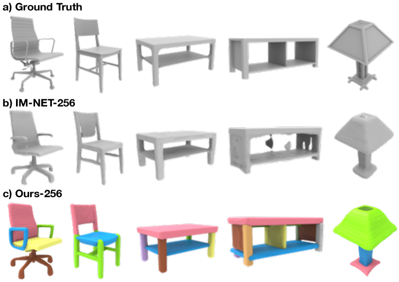
Figure 4: Visual results for shape auto-encoding. Output meshes are obtained using the same marching cubes setup.

4.2 Shape Generation and Interpolation

We compare to two state-of-the-art 3D shape generative models, IM-NET [10] and StructureNet [36], for 3D shape generation task. We use the released code for both method. For IM-NET, we retrain their model on all three category. For StructureNet, we use the pre-trained models on Chair and Table, and retrain the model for Lamp category.

Category	Method	COV	MMD	JSD
Chair	Ours	54.91	8.34	0.0083
	IM-NET	52.35	7.44	0.0084
	StructureNet	29.51	9.67	0.0477
Table	Ours	56.51	7.56	0.0057
	IM-NET	56.67	6.90	0.0047
	StructureNet	16.04	14.98	0.0725
Lamp	Ours	87.95	10.01	0.0215
	IM-NET	81.25	10.45	0.0230
	StructureNet	35.27	17.29	0.1719

Table 2: Quantitative evaluation for shape generation. We randomly generated 2000 shapes for each method and then compared to the test dataset. COV and MMD use chamfer distance as distance measure. MMD is multiplied by $10^{3}$.

We adopt Coverage (COV), Minimum Matching Distance (MMD) and Jensen-Shannon Divergence (JSD) [1] to evaluate the fidelity and diversity of generation results. While COV and JSD roughly represent the diversity of the generated shapes, MMD is often used for fidelity evaluation. We obtained a set of generated shapes for each method by randomly generating 2K samples and compare to the test set using chamfer distance. More details about evaluation metrics are available in supplementary material.

The results of PQ-NET and IM-NET are sampled at resolution $256^{3}$ for visual comparison and $64^{3}$ for quantitative evaluation. We reconstruct the mesh and sample 2K points to calculate chamfer distance. Since StructureNet outputs 1K points for each generated part, the whole shape may contain points larger than 2K. We conduct a downsampling process to extract 2K points for evaluation.

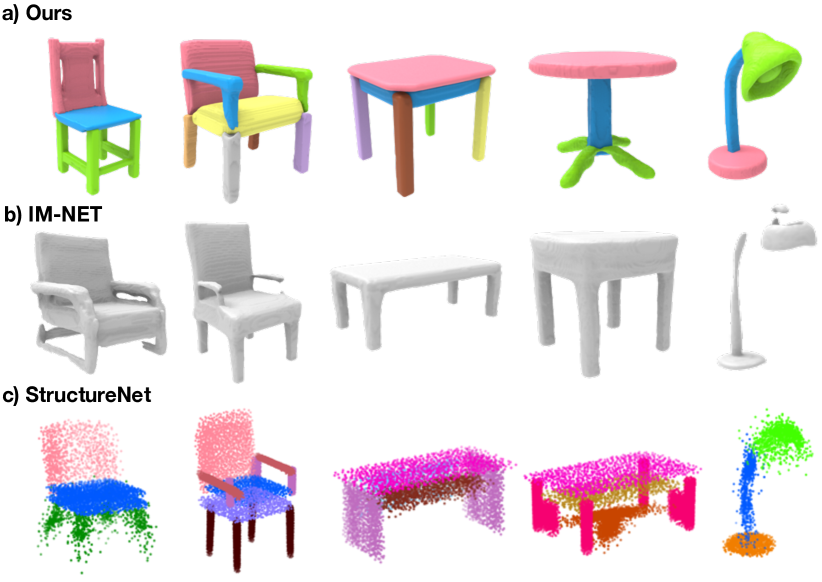
Figure 5: 3D shape generation results with comparison to results obtained by IM-NET and StructureNET.

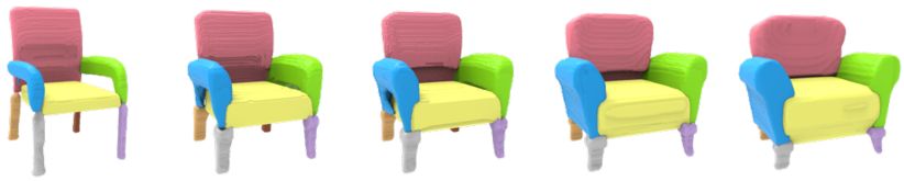
Figure 6: Latent space interpolation results. The interpolated sequence not only consists of smooth geometry morphing but also keeps the shape structure.

Table 2 and Figure 5 shows the results from our PQ-NET, IM-NET and StructureNet. Our method can produce smooth geometry while maintaining the whole structure preserved. For thin structure and complex topology, modeling whole shape is very hard, and our decomposition strategy can be very helpful in such hard situation. However, on the other hand, our sequential model may yield duplicated parts or miss parts sometimes. As to get the sufficient generative model, it is important to balance the hardness between geometry generation and structure recovery.

Besides random generation, we also show interpolation results in Figure 6. Interpolation between latent vector is a way to show the continuity of learned shape latent space. Linear interpolation from our latent space yields smooth transiting shapes in terms of geometry and structure.

4.3 Comparison to 3D-PRNN

Since 3D-PRNN [58] is the most related work, we conduct a comprehensive comparison with them. We first compare the reconstruction task from a single depth image by evaluating only the structure of shape, since 3D-PRNN doesn’t recover shape geometry. For each 3D shape in the dataset, we obtain 5 depth maps by the resolution of $64^{2}$. We uniformly sample 5 views and render the depth images using ground truth mesh. For both 3D-PRNN and our model, we use part axis aligned bounding box(AABB) as structure representation. In addition, 3D-PRNN uses a pre-sort order from the input parts. Therefore, besides using the natural order from PartNet annotations, we also train the model on the top-town order used by 3D-PRNN.

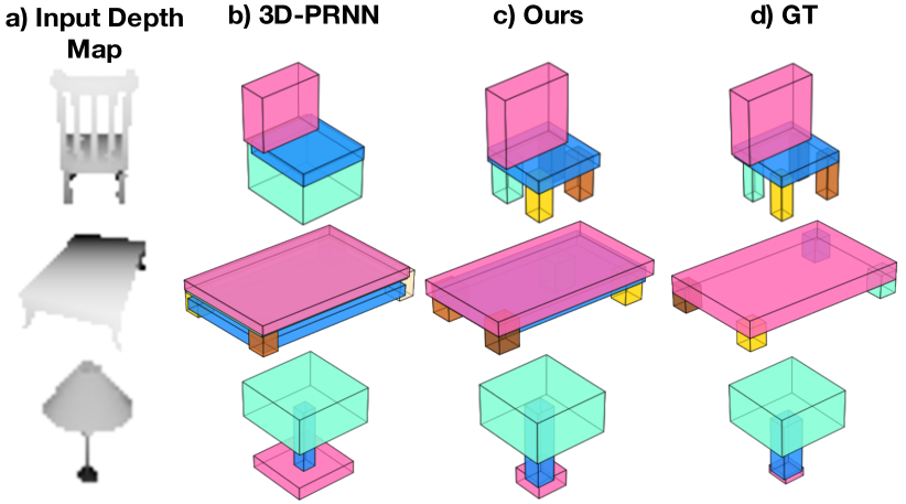
Figure 7: Visual comparison of structured 3D shape reconstruction from single depth image on three categories: chair, table, lamp.

Figure 7 shows the visual comparison between our PQ-NET and 3D-PRNN. Our method can reconstruct much plausible boxes. For quantitative evaluation, we convert the output and ground truth boxes to volumetric model by fully filling with each part box, and compute IoU between generated model and the corresponding ground truth volume. As a result, our reconstructed structures are more accurate, as shown in Table 3. In terms of order effect, our model on the natural order of PartNet yields the best result. The quality drops down with small portion when using the top-down order as 3D-PRNN, however is still better than theirs.

Method	Order	Chair	Table	Lamp	Average
Ours	A	61.47	53.67	52.94	56.03
	B	58.68	48.58	52.17	53.14
3D-PRNN	A	37.26	51.30	47.26	45.27
	B	36.46	51.93	43.83	44.07

Table 3: Shape IoU evaluation of structured 3D shape reconstruction from single depth image on three categories: chair, table, lamp. We test each method on two kinds of order: PartNet natural order(A) and presorted top-down order(B).

We also compare the 3D shape generation task with 3D-PRNN, as shown in Figure 8. Quantitative evaluation and more details can be found in supplementary material.

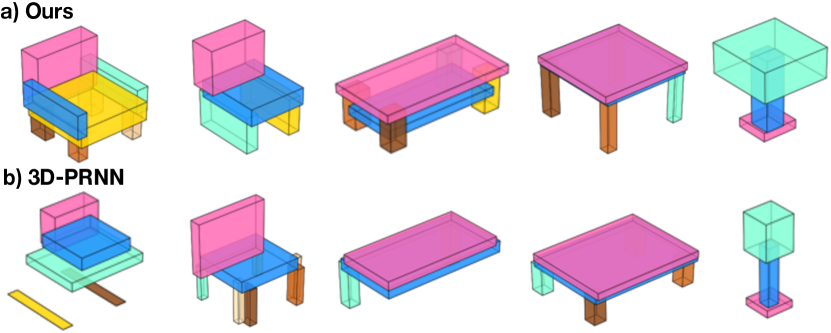
Figure 8: Visual comparison of random generated 3D primitives. 3D-PRNN suffers from unreal, duplicated or missing parts while our model can yield more plausible results.

4.4 Single View 3D Reconstruction

We compare our approach with IM-NET  [11] on the task of single view reconstruction from RGB image. We per-category trained IM-NET on PartNet dataset. Figure 9 shows the results. It can be seen that our approach can recover more complete and detailed geometry than IM-NET. The advantage of model is that we also obtain segmentation besides reconstructed geometry. However, relying on the structure information may cause issues, such as duplicated or misplaced part, see the first table in Figure 9(c).

We admit our method doesn’t outperform IM-NET in the quantitative evaluation. This may due to the fact that our latent space is entangled with both the geometry and structure, which makes the latent space less uniform.

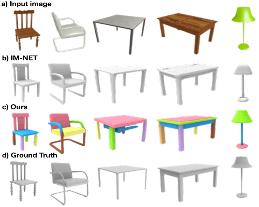
Figure 9: Single view reconstruction results. Our results are from model that is trained across all three category. Note that our method also recovers the shape structure.

4.5 Applications

By altering the training procedure applied to our network, we show that PQ-NET can serve two more applications which benefit from sequential part assembly.

Shape completion.

We can train our network by feeding it input part sequences which constitute a partial shape, and force the network to reconstruct the full sequence, hence completing the shape. We tested this idea on the chair category, by randomly removing up to $k-1$ parts from the part sequence, $k$ being the total number of parts of a given shape. One result is shown in Figure 1 with more available in the supplementary material.

Order denoising and part correspondence.

We can add “noise” to a part order by scrambling it, feed the resulting noisy order to our network, and force it to reconstruct the original (clean) order. We call this procedure part order denoising — it allows the network to learn a consistent part order for a given object category, e.g., chairs, as long as we provide the ground truth orders with consistency. For example, we can enforce the order “back $\rightarrow$ seat $\rightarrow$ legs” and for the legs, we order them in clockwise order. If all the part orders adhere to this, then it should be straightforward to imply a part correspondence, which can, in turn, facilitate inference of part relations such as symmetry; see Figure 10.

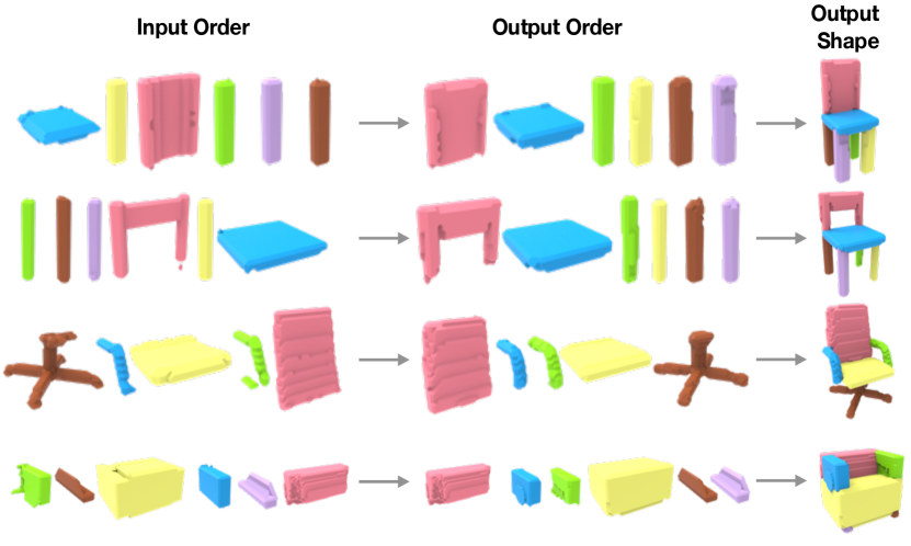
Figure 10: Part order denoising results. Our method can unscramble random input orders into a consistent output order, to facilitate part correspondence. Note that the color correspondence is for illustrations only, and not part of the output from our network.

With structural variaties, it still requires some work to infer the part correspondence from all possible (consistent) linear part sequences; this is beyond the scope of our current work. It is worth noting however that this inference problem would be a lot harder if the parts are organized hierarchically [53, 31, 36] rather than linearly.

5 Conclusion, limitation, and future work

We present PQ-NET, a deep neural network which represents and generates 3D shapes as an assembly sequence of parts. The generation can be from random noise to obtain novel shapes or conditioned on single-view depth scans or RGB images for 3D reconstruction. Promising results are demonstrated for various applications and in comparison with state-of-the-art generative models of 3D shapes including IM-NET [10], StructureNet [36], and 3D-PRNN [58], where the latter work also generates part assemblies.

One key limitation of PQ-NET is that it does not learn part relations such as symmetry; it only outputs a spatial arrangement of shape parts. More expressive structural representations such as symmetry hierarchies [53, 31] and graphs [36] can encode such relations easily. However, to learn such representations, one needs to prepare sufficient training data which is a non-trivial task. The part correspondence application shown in Section 4.5 highlights an advantage of sequential representations, but in general, an investigation into the pros and cons of sequences vs. hierarchies for learning generative shape models is worthwhile. Another limitation is that PQ-NET does not produce topology-altering interpolation, especially between shapes with different number of parts. Further investigation into latent space formed by sequential model is needed.

We would also like to study more closely the latent space learned by our network, which seems to be encoding part structure and geometry in an entangled and unpredictable manner. This might explain in part why the 3D reconstruction quality from PQ-NET still does not quite match that of state-of-the-art implicit models such as IM-NET. Finally, as shown in Table 3, part orders do seem to impact the network learning. Hence, rather than adhering to a fixed part order, the network may learn a good, if not the optimal, part order, for different shape categories, i.e., the best assembly sequence. An intriguing question is what would be an appropriate loss to quantify the best part order.

Supplementary Materials

A Overview

This supplementary material contains six parts:

• Sec.B describes the implementation detailed of our PQ-NET.

• Sec.C describes the data preparation details.

• Sec.D explains the metrics used for the evaluation of shape generation.

• Sec.E provides comparison results to 3D-PRNN on generation task.

• Sec.F provides more visual results of partial shape completion, random shape generation.

B Implementation Details

We describe the detailed implementation of our PQ-NET architecture along with the training configuration.

CNN Encoder
Layer	Kernel Size	Stride	Output Shape
input voxel	-	-	(1,64,64,64)
Conv3D+BN+lReLU	(4,4,4)	(2,2,2)	(32,32,32,32)
Conv3D+BN+lReLU	(4,4,4)	(2,2,2)	(64,16,16,16)
Conv3D+BN+lReLU	(4,4,4)	(2,2,2)	(128,8,8,8)
Conv3D+BN+lReLU	(4,4,4)	(2,2,2)	(256,4,4,4)
Conv3D+Sigmoid	(4,4,4)	(1,1,1)	(128,1,1,1)
Implicit Decoder
Layer	Dropout	Input Shape	Output Shape
feature+coordinates	-	(128 + 3)	(131)
FC+lReLU	0.4	(131)	(2048)
FC+lReLU	0.4	(2048 + 131)	(1024)
FC+lReLU	0.4	(1024 + 131)	(512)
FC+lReLU	0.4	(512 + 131)	(256)
FC+lReLU	-	(256 + 131)	(128)
FC+Sigmoid	-	(128)	(1)

Table 4: Architecture of our part geometry autoencoder. Conv3D: 3D Convolutional Layer, BN: Batch Normalization, lReLU: leaky ReLU, FC: Fully Connected Layer.

Seq2Seq Encoder RNN
Type	#layers	input size	hidden size	bidirectional
GRU	2	(128+6+K)	256	True
Seq2Seq Decoder RNN
Type	#layers	input size	hidden size	bidirectional
GRU	2	(128+6)	512	False
Seq2Seq Decoder FC
Type		input size	hidden size	output size
FC-lReLU-FC		512	256	128
FC-ReLU-FC		512	128	6
FC-ReLU-FC		512	128	1

Table 5: Architecture of our Seq2Seq autoencoder. K is the maximum number of parts of all shaeps in the dataset.

Table 5 and Table 5 list the detailed architecture with specific parameters of our PQ-NET, divided into part geometry autoencoder and Seq2Seq autoencoder. For part geometry autoencoder, we use similar design as IM-NET  [10], with skip connection in the implicit decoder. For Seq2Seq autoencoder, we also employ dropout regularization with drop rate $0.2$ in the middle of GRU to reduce overfitting.

As mentioned in the main paper, we train our PQ-NET in two separate steps. We adopt a progressive strategy to train our part geometry autoencoder by increasing the resolution of part volum. Practically, we use resolution of $16^{3}$, $32^{3}$ and $64^{3}$ with batch size $40$ and learning rate 5e-4 in our experiments. Then the part geometry autoencoder is fixed and used to train the Seq2Seq autoencoder on the resolution of $64^{3}$ with batch size as 64 and learning rate as 1e-3. We use PyTorch [paszke2017automatic] framework to implement our PQ-NET and conduct all the experiments.

C Data Preparation Details

For all experiments in our paper, we mainly use three largest categories of PartNet [37], that is, chair, table and lamp. Since each shape in PartNet is partitioned into small elements and then grouped following a hierarchical structure with each node a semantical label, we use the nodes in the second layer as our part geometry. The part label we used appears in the file ”partnet-dataset$\backslash$stats$\backslash$after_merging_label_ids$\backslash$xxx-label-2.txt”, where ”xxx” correspondes to the number of each shape categories. We remove shapes that contain more than 10 parts, resulting in 6305 chairs, 7357 tables and 1188 lamps, which are further divided into training, validation and test sets using official data splits of PartNet. Note that this upper bound of number of parts can be increased. Table 6 shows the statistics result about the number of parts per shape in our dataset.

	Chair	Table	Lamp
avg #parts	5.59	6.06	2.94
min #parts	2	2	2
max #parts	9	10	7

Table 6: Average, minimum and maximum number of parts per shape for each category in our dataset.

To prepare the training data for our network, we first voxelize the original shape mesh into voxel representation at $64^{3}$ resolution and fill the interior of the shape voxel using classic flood filling algorithm. Each part is then scaled to $64^{3}$ resolution within its bounding box. The resulting $64^{3}$ part volums are downsampled to $32^{3}$ and $16^{3}$ resolution. With voxelized part geometry at differ resolutions, we follow the sampling approach as in IM-NET to progressively sample points near the surface with each point a signed distance to the surface. Specifically, we sample $4096$ points in $16^{3}$ volum, and with higher resolutions, such as $32^{3}$ and $64^{3}$, we sample $8192$ and $32768$, respectively. The sampled points together with signed distance values are used to train our part geometry autoencoder. The box parameters used in Seq2Seq autoencoder training are produced by calculating bounding box of each part in original shape voxel. Intuitively, the box parameters indicate the deviation and translation from part local frame to the shape coordinate system.

D Metrics

We explain the quantitative metrics adopt for generation task in our paper, i.e. Coverage (COV), Minimum Matching Distance (MMD) and Jensen-Shannon Divergence (JSD) . In their calculation, chamfer distance is used when comparing our method to IM-NET [10] and StructureNet [36] while IoU is used when comparing to 3D-PRNN [58]. Let $\mathcal{G}$ be a set of generated shapes and $\mathcal{S}$ be the ground truth test set:

COV

To compute COV, for each shape in $\mathcal{G}$ we find its nearest neighbor in $\mathcal{S}$ and mark it as matched. COV is the fraction of matched shapes in $\mathcal{S}$ over the total size of $\mathcal{S}$. COV roughly represents the diversity of the generated shapes. A high COV score suggests most of shapes in $\mathcal{S}$ can be roughly represented by shapes in $\mathcal{G}$.

MMD

To compute MMD, for each shape in $\mathcal{S}$, we calculate the distance to its nearest neighbor in $\mathcal{G}$. Then MMD is defined as the average of all these distances. MMD roughly represents the fidelity of the generated shapes.

JSD

In a predefined voxel gird, for each shape in point cloud form in $\mathcal{G}$, we count the number of points lying inside each voxel, and do the same for $\mathcal{S}$. Then we get two distribution in Euclidean 3D space $P_{\mathcal{G}}$ and $P_{\mathcal{S}}$. JSD is defined as the Jensen-Shannon Divergence between two distributions.

We use the code from https://github.com/optas/latent_3d_points for calculation.

E Comparison to 3D-PRNN on Shape Generation Task

In this section, we demonstrate detailed comparison results to 3D-PRNN [58] on shape generation task, which are not fully shown in the main paper due to paper length limitation. Unlike our PQ-NET that generates new shapes from random noise, 3D-PRNN samples new structure within a constraint region. For a fair comparison, we follow the setting described in their paper, by sampling the first input feature of RNN from training data.

Metrics	Method	Chair	Table	Lamp	Avg
COV-IoU	Ours	58.94	59.80	76.34	65.03
	3D-PRNN	51.03	36.44	58.93	48.80
MMD-IoU	Ours	0.259	0.271	0.298	0.276
	3D-PRNN	0.275	0.357	0.347	0.326

Table 7: Quantitative comparison on 3D shape generation.

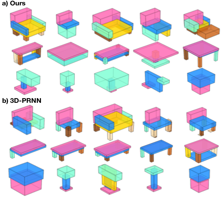
Figure 11: More visual comparison of random generated 3D primitives between ours and 3D-PRNN.

Results of quantitative comparison on are shown in and Table 7. We sampled 2000 random generated shapes for chair and table, 800 for lamp, to compute the coverage(COV) and minimum matching distance(MMD) between the generated set and ground truth test set. We use $1-\text{IoU}$ as the distance measure when comparing two shapes. It can be seen that our network outperforms 3D-PRNN in all of the measurements, which means that our generation results are more diverse and plausible. More visual results are shown in Figure 11.

F More Results

Figure 12 shows visual results for partial shape completion and Figure 13 at the last page shows more results of our generated shapes.

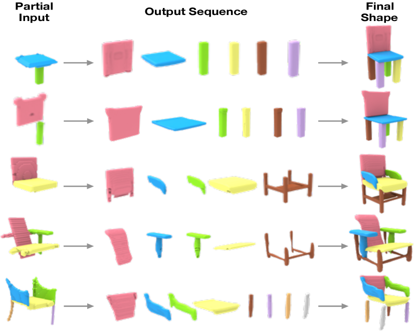
Figure 12: Visual results of partial shape completion.

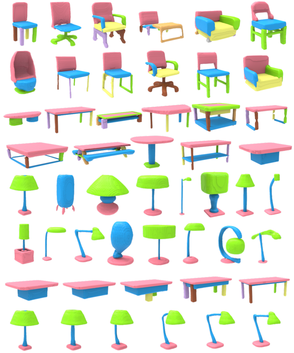
Figure 13: More visual results of our generated shapes (row 1-6), along with two latent space interpolation (row 7-8). All shapes are sampled at resolution $256^{3}$ and reconstructed using Marching Cubes.

References

- [1] P. Achlioptas, O. Diamanti, I. Mitliagkas, and L. Guibas. Learning representations and generative models for 3d point clouds. arXiv preprint arXiv:1707.02392, 2018.
- [2] B. Allen, B. Curless, and Z. Popović. The space of human body shapes: Reconstruction and parameterization from range scans. ACM Trans. Graph., 22(3), 2003.
- [3] M. Arjovsky, S. Chintala, and L. Bottou. Wasserstein generative adversarial networks. In D. Precup and Y. W. Teh, editors, Proceedings of the 34th International Conference on Machine Learning, volume 70 of Proceedings of Machine Learning Research, pages 214–223, International Convention Centre, Sydney, Australia, 06–11 Aug 2017. PMLR.
- [4] A. Arsalan Soltani, H. Huang, J. Wu, T. D. Kulkarni, and J. B. Tenenbaum. Synthesizing 3d shapes via modeling multi-view depth maps and silhouettes with deep generative networks. In Proc. CVPR, pages 1511–1519, 2017.
- [5] I. Biederman. Recognition-by-components: A theory of human image understanding. Psychological Review, 94(2):115–147, 1987.
- [6] V. Blanz and T. Vetter. A morphable model for the synthesis of 3D faces. In Proc. of SIGGRAPH, pages 187–194, 1999.
- [7] R. D. Borsley. Modern phrase structure grammar. 1996.
- [8] A. X. Chang, T. Funkhouser, L. J. Guibas, P. Hanrahan, Q. Huang, Z. Li, S. Savarese, M. Savva, S. Song, H. Su, J. Xiao, L. Yi, and F. Yu. ShapeNet: An Information-Rich 3D Model Repository. (arXiv:1512.03012 [cs.GR]), 2015.
- [9] D.-Y. Chen, X.-P. Tian, Y.-T. Shen, and M. Ouhyoung. On visual similarity based 3d model retrieval. Computer Graphics Forum, 22(3):223–232, 2003.
- [10] Z. Chen and H. Zhang. Learning implicit fields for generative shape modeling. Proceedings of IEEE Conference on Computer Vision and Pattern Recognition (CVPR), 2019.
- [11] Z. Chen and H. Zhang. Learning implicit fields for generative shape modeling. In CVPR, 2019.
- [12] K. Cho, B. van Merrienboer, Ç. Gülçehre, F. Bougares, H. Schwenk, and Y. Bengio. Learning phrase representations using RNN encoder-decoder for statistical machine translation. CoRR, abs/1406.1078, 2014.
- [13] C. B. Choy, D. Xu, J. Gwak, K. Chen, and S. Savarese. 3d-r2n2: A unified approach for single and multi-view 3d object reconstruction. In European conference on computer vision, pages 628–644. Springer, 2016.
- [14] A. Dubrovina, F. Xia, P. Achlioptas, M. Shalah, and L. Guibas. Composite shape modeling via latent space factorization. arXiv preprint arXiv:1803.10932, 2019.
- [15] H. Fan, H. Su, and L. Guibas. A point set generation network for 3D object reconstruction from a single image. arXiv preprint arXiv:1612.00603, 2016.
- [16] H. Fan, H. Su, and L. J. Guibas. A point set generation network for 3d object reconstruction from a single image. In Proc. CVPR, pages 605–613, 2017.
- [17] N. Fish, M. Averkiou, O. Van Kaick, O. Sorkine-Hornung, D. Cohen-Or, and N. J. Mitra. Meta-representation of shape families. ACM Transactions on Graphics (TOG), 33(4):34, 2014.
- [18] L. Gao, J. Yang, T. Wu, Y.-J. Yuan, H. Fu, Y.-K. Lai, and H. Zhang. Sdm-net: Deep generative network for structured deformable mesh. arXiv preprint arXiv:1908.04520, 2019.
- [19] R. Girdhar, D. F. Fouhey, M. Rodriguez, and A. Gupta. Learning a predictable and generative vector representation for objects. In European Conference on Computer Vision, pages 484–499. Springer, 2016.
- [20] T. Groueix, M. Fisher, V. G. Kim, B. C. Russell, and M. Aubry. A papier-mâché approach to learning 3d surface generation. In Proc. CVPR, pages 216–224, 2018.
- [21] I. Gulrajani, F. Ahmed, M. Arjovsky, V. Dumoulin, and A. Courville. Improved training of wasserstein gans. In Proceedings of the 31st International Conference on Neural Information Processing Systems, NIPS’17, pages 5769–5779, USA, 2017. Curran Associates Inc.
- [22] K. He, X. Zhang, S. Ren, and J. Sun. Deep residual learning for image recognition. In Proceedings of the IEEE conference on computer vision and pattern recognition, pages 770–778, 2016.
- [23] G. Hinton, A. Krizhevsky, N. Jaitly, T. Tieleman, and Y. Tang. Does the brain do inverse graphics? In Brain and Cognitive Sciences Fall Colloquium, 2012.
- [24] D. D. Hoffman and W. A. Richards. Parts of recognition. Cognition, pages 65–96, 1984.
- [25] H. Huang, E. Kalogerakis, and B. Marlin. Analysis and synthesis of 3d shape families via deep-learned generative models of surfaces. Computer Graphics Forum, 34(5), 2015.
- [26] E. Kalogerakis, S. Chaudhuri, D. Koller, and V. Koltun. A Probabilistic Model of Component-Based Shape Synthesis. ACM Transactions on Graphics, 31(4), 2012.
- [27] V. G. Kim, W. Li, N. J. Mitra, S. Chaudhuri, S. DiVerdi, and T. Funkhouser. Learning part-based templates from large collections of 3D shapes. ACM Transactions on Graphics (Proc. SIGGRAPH), 32(4), July 2013.
- [28] R. Klokov, J. Verbeek, and E. Boyer. Probabilistic reconstruction networks for 3d shape inference from a single image. In BMVC, 2019.
- [29] T. D. Kulkarni, W. F. Whitney, P. Kohli, and J. Tenenbaum. Deep convolutional inverse graphics network. In Advances in Neural Information Processing Systems (NIPS), 2015.
- [30] J. Li, C. Niu, and K. Xu. Learning part generation and assembly for structure-aware shape synthesis. arXiv preprint arXiv:1906.06693, 2019.
- [31] J. Li, K. Xu, S. Chaudhuri, E. Yumer, H. Zhang, and L. Guibas. Grass: Generative recursive autoencoders for shape structures. arXiv preprint arXiv:1705.02090, 2017.
- [32] X. Liu, Z. Han, Y.-S. Liu, and M. Zwicker. Point2sequence: Learning the shape representation of 3d point clouds with an attention-based sequence to sequence network. In Proceedings of the AAAI Conference on Artificial Intelligence, volume 33, pages 8778–8785, 2019.
- [33] Z. Lun, M. Gadelha, E. Kalogerakis, S. Maji, and R. Wang. 3d shape reconstruction from sketches via multi-view convolutional networks. In 2017 International Conference on 3D Vision (3DV), pages 67–77. IEEE, 2017.
- [34] P. Mandikal, N. KL, and R. Venkatesh Babu. 3d-psrnet: Part segmented 3d point cloud reconstruction from a single image. In Proceedings of the European Conference on Computer Vision (ECCV), pages 0–0, 2018.
- [35] L. Mescheder, M. Oechsle, M. Niemeyer, S. Nowozin, and A. Geiger. Occupancy networks: Learning 3D reconstruction in function space. In Proc. CVPR, 2019.
- [36] K. Mo, P. Guerrero, L. Yi, H. Su, P. Wonka, N. Mitra, and L. J. Guibas. Structurenet: Hierarchical graph networks for 3d shape generation. ACM Trans. on Graph. (SIGGRAPH Asia), 2019.
- [37] K. Mo, S. Zhu, A. X. Chang, L. Yi, S. Tripathi, L. J. Guibas, and H. Su. PartNet: A large-scale benchmark for fine-grained and hierarchical part-level 3D object understanding. In The IEEE Conference on Computer Vision and Pattern Recognition (CVPR), June 2019.
- [38] C. Nash and C. K. Williams. The shape variational autoencoder: A deep generative model of part-segmented 3d objects. Computer Graphics Forum (SGP 2017), 36(5):1–12, 2017.
- [39] C. Niu, J. Li, and K. Xu. Im2struct: Recovering 3d shape structure from a single rgb image. In Proceedings of the IEEE Conference on Computer Vision and Pattern Recognition, pages 4521–4529.
- [40] M. Ovsjanikov, W. Li, L. Guibas, and N. J. Mitra. Exploration of continuous variability in collections of 3d shapes. ACM Trans. on Graph. (SIGGRAPH), 30(4):33:1–33:10, 2011.
- [41] J. J. Park, P. Florence, J. Straub, R. Newcombe, and S. Lovegrove. DeepSDF: Learning continuous signed distance functions for shape representation. In CVPR, 2019.
- [42] S. R. Richter and S. Roth. Matryoshka networks: Predicting 3d geometry via nested shape layers. CoRR, abs/1804.10975, 2018.
- [43] G. Riegler, A. O. Ulusoy, and A. Geiger. Octnet: Learning deep 3d representations at high resolutions. In Proc. CVPR, volume 3, 2017.
- [44] N. Schor, O. Katzier, H. Zhang, and D. Cohen-Or. Learning to generate the ”unseen” via part synthesis and composition. In IEEE International Conference on Computer Vision, 2019.
- [45] M. Schuster and K. K. Paliwal. Bidirectional recurrent neural networks. IEEE Transactions on Signal Processing, 45(11):2673–2681, 1997.
- [46] A. A. Soltani, H. Huang, J. Wu, T. D. Kulkarni, and J. B. Tenenbaum. Synthesizing 3d shapes via modeling multi-view depth maps and silhouettes with deep generative networks. In Proceedings of the IEEE Conference on Computer Vision and Pattern Recognition, pages 1511–1519, 2017.
- [47] I. Sutskever, O. Vinyals, and Q. V. Le. Sequence to sequence learning with neural networks. In Advances in neural information processing systems, pages 3104–3112, 2014.
- [48] M. Tatarchenko, A. Dosovitskiy, and T. Brox. Octree generating networks: Efficient convolutional architectures for high-resolution 3d outputs. In IEEE International Conference on Computer Vision (ICCV), 2017.
- [49] S. Tulsiani, H. Su, L. J. Guibas, A. A. Efros, and J. Malik. Learning shape abstractions by assembling volumetric primitives. In Proc. CVPR, pages 2635–2643, 2017.
- [50] H. Wang, N. Schor, R. Hu, H. Huang, D. Cohen-Or, and H. Huang. Global-to-local generative model for 3d shapes. ACM Transactions on Graphics (Proc. SIGGRAPH ASIA), 37(6):214:1—214:10, 2018.
- [51] N. Wang, Y. Zhang, Z. Li, Y. Fu, W. Liu, and Y.-G. Jiang. Pixel2mesh: Generating 3d mesh models from single rgb images. In ECCV, pages 52–67, 2018.
- [52] P.-S. Wang, Y. Liu, Y.-X. Guo, C.-Y. Sun, and X. Tong. O-CNN: Octree-based Convolutional Neural Networks for 3D Shape Analysis. ACM Transactions on Graphics (SIGGRAPH), 36(4), 2017.
- [53] Y. Wang, K. Xu, J. Li, H. Zhang, A. Shamir, L. Liu, Z. Cheng, and Y. Xiong. Symmetry hierarchy of man-made objects. Computer Graphics Forum, 30(2):287–296, 2011.
- [54] J. Wu, C. Zhang, T. Xue, B. Freeman, and J. Tenenbaum. Learning a probabilistic latent space of object shapes via 3d generative-adversarial modeling. In Advances in Neural Information Processing Systems, pages 82–90, 2016.
- [55] Z. Wu, X. Wang, D. Lin, D. Lischinski, D. Cohen-Or, and H. Huang. Structure-aware generative network for 3d-shape modeling. arXiv preprint arXiv:1808.03981, 2018.
- [56] Q. Xu, W. Wang, D. Ceylan, R. Mech, and U. Neumann. DISN: deep implicit surface network for high-quality single-view 3d reconstruction. CoRR, abs/1905.10711, 2019.
- [57] G. Yang, X. Huang, Z. Hao, M.-Y. Liu, S. Belongie, and B. Hariharan. Pointflow: 3d point cloud generation with continuous normalizing flows. arXiv, 2019.
- [58] C. Zou, E. Yumer, J. Yang, D. Ceylan, and D. Hoiem. 3D-PRNN: Generating shape primitives with recurrent neural networks. 2017 IEEE International Conference on Computer Vision (ICCV), Oct 2017.