An Investigation on Semismooth Newton based Augmented Lagrangian Method for Image Restoration
Abstract
Augmented Lagrangian method (also called as method of multipliers) is an important and powerful optimization method for lots of smooth or nonsmooth variational problems in modern signal processing, imaging, optimal control and so on. However, one usually needs to solve the coupled and nonlinear system together and simultaneously, which is very challenging. In this paper, we proposed several semismooth Newton methods to solve the nonlinear subproblems arising in image restoration in finite dimensional spaces, which leads to several highly efficient and competitive algorithms for imaging processing. With the analysis of the metric subregularities of the corresponding functions, we give both the global convergence and local linear convergence rate for the proposed augmented Lagrangian methods with semismooth Newton solvers.
1 Introduction
The augmented Lagrangian method (shorted as ALM henceforth) was originated in [13, 26]. The early developments can be found in [3, 11, 30] and the extensive studies in infinite dimensional spaces with various applications can be found in [11, 20] and so on. The comprehensive studies of ALM for convex, nonsmooth optimization and variational problems can be found in [3, 20]. In [30], the celebrated connections between the ALM and proximal point algorithms are established, where ALM is found to be equivalent to the proximal point algorithm applying to the essential dual problem. The convergence can thus be concluded in the general and powerful proximal point algorithm framework for convex optimization [29, 30].
ALM is very flexible for constrained optimization problems including both equality and inequality constraint problems [3, 20]. However, the challenging problem is solving the nonlinear and coupling systems simultaneously which usually appear while applying ALM. This is different from alternating direction method of multipliers (ADMM) type methods [12, 11], which decouple the unknown variables, deal with each subproblem separately and update them consecutively. However, for ALM, the extra effort is deserved if the nonlinear systems can be solved efficiently. This is due to the appealing asymptotic linear or superlinear convergence of ALM with increasing step sizes [29, 30, 25]. It is well known semismooth Newton methods are efficient solvers for nonsmooth and nonlinear systems. Semismooth Newton based augmented Lagrangian methods already have lots of successful applications in semidefinite programming [42], compressed sensing [24, 41], friction and contact problem [33, 34] and imaging problems [14, 21].
In this paper, we proposed several novel semismooth Newton based augmented Lagrangian methods for the total variation regularized image restoration problems with quadratic data terms. Total variation (TV) regularization is quite fundamental for imaging problems. Besides, the regularization problem is a typical nonsmooth and convex optimization problem which is very challenging to solve and is standard for testing various algorithms [4]. To the best of our knowledge, the most related work is [14, 21, 16]. In [14], Moreau-Yosida regularized dual problem of the anisotropic ROF model in Banach space is considered and solved with the semismooth Newton based ALM method. In [21], the primal-dual active set method is employed for nonlinear systems of the ALM applying to the additionally regularized primal problems for solving the nonlinear system. In [16], semismooth Newton methods are directly applied to the strongly convex regularized ROF models with strong convexity on both the primal and dual variables without ALM method.
All the proposed algorithms are based on applying ALM to the primal model, whose strong convexity can be employed. Compared to [16], we do not need the strong convexity on the dual variables. Our contributions belong to the following parts. First, by introducing auxiliary variables, we use primal-dual semismooth Newton method [16] for nonlinear systems of ALM, which is very efficient for ALM. The proposed ALM is very efficient compared to the popular existing algorithms including the primal-dual first-order method [4]. They are especially very fast for the anisotropic total variation regularized quadratic problems. Second, we proved that the maximal monotone KKT (Kuhn-Tucker) mapping is metric subregular for the anisotropic TV regularized quadratic problem. We thus get the asymptotic linear or superlinear convergence rate of both the primal and dual sequence for the anisotropic case by the framework in [29, 30, 25]. With the calm intersection theorem [18], we also prove the metric subregularity of the maximal monotone operator associated with the dual problem for the isotropic case under mild condition. This leads to the asymptotic linear or superlinear convergence rate of the dual sequence for the isotropic case [29, 30, 25]. To the best of our knowledge, these subregularities are novel for the TV regularized quadratic problems. Third, we also give a systematical investigation of another efficient semismooth Newton method for solving the nonlinear systems that appear in ALM, which is involved with the soft thresholding operator.
The rest of this paper is organized as follows. In section 2, we give an introduction to the TV regularized quadratic problems and the corresponding ALM including the isotropic and anisotropic cases. In section 3, we present discussions on the primal-dual semismooth Newton for ALM by introducing auxiliary variables, which turns out very efficient. In section 4, we give detailed discussions on the semismooth Newton method involving the soft thresholding operators. Although all the semismooth Newton algorithms are aiming at the same nonlinear system for the isotropic or the anisotropic TV regularization. However, different formulations turn out different algorithms with efficiency. In section 5, we give the metric subregularity for the maximal monotone KKT mapping for anisotropic TV regularized quadratic problems and for the maixmal monotone operator associated with the dual problem of isotropic TV regularized quadratic problems. Together with the convergence of the semismooth Newton method, we get the corresponding asymptotic linear convergence. In section 6, we present the detailed numerical tests for all the algorithms and the comparison with efficient first-order algorithms focused on the ROF model and deblurring model. In section 7, we present some discussions.
2 Image restoration and Augmented Lagrangian Methods
The total variation regularized model is as follows.
| (P) |
where with and being the known data for general image restoration [16, 21]. Here is a linear and bounded operator depending on the problems, e.g., being the convolution with kernel for image deblurring problems. The strong convexity of is of critical importance for the proposed algorithms and analysis. Especially, the ROF model is for the case and . For the deblurring problems, we added the strongly regularization term with since is usually not positive definite. Henceforth, all the variables, operators and spaces are all in finite dimensional space setting. The norm based on the following isotropic or anisotropic norm
| (2.1) |
where . We denote as the Euclidean norm including the absolute value for real valued scalar. Now introduce the image domain which is the discretized grid [4]
where are the image dimensions. With discrete image domain , we define the discrete image space as with the standard scalar product. Finite differences are used to discretize the operator and its adjoint operator with homogeneous Neumann and Dirichlet boundary conditions, respectively. We define as the following operator
where forward differences are taken according to
With with the standard product scalar product, this gives a linear operator . The discrete divergence is then the negative adjoint of with , i.e., the unique linear mapping which satisfies for ,
| (2.2) |
where the inner products are defined by
The operator can be computed as and we refer to [4] for the detailed backward difference operators and .
By (2.1), the isotropic or anisotropic TV in (P) is as follows,
| (2.3) |
where in (2.3) is the area element of and the integrals in (2.3) are understood as the finite summation over all pixels. With these preparations, by the Fenchel-Rockafellar duality theory [2, 20], the primal-dual form of (P) can be written as
| (2.4) |
where is the indicator function and the dual form of (P) can be written
| (D) |
The notations and the positive definite, linear operator are as follows
| (2.5) |
We also need the following norms for arbitrary , , ,
The is defined as follows. For the isotropic case,
For the anisotropic case, with (2.3) and applying the Fenchel-Rockafellar duality theory for and separately, we have
The optimality conditions on the saddle points are as follows
| (2.6) |
By the Fenchel-Rockafellar duality theory, we have and
| (2.7) |
The optimality condition for in (2.6) is also equivalent to
| (2.8) |
where is the projection to the feasible set , i.e.,
| (2.9) |
Introducing , the problem (P) becomes the following constrained optimization problem
The augmented Lagrangian method thus follows, with nondecreasing update of ,
| (2.10) | ||||
| (2.11) |
We will use the semismooth Newton method to solve (2.10). The optimality conditions with fixed and for (2.10) are
| (2.12) | |||
| (2.13) |
where are the optimal solutions of (2.10). The equation (2.13) leads to
| (2.14) |
where is the soft thresholding operator for the isotropic or anisptropic norm. With relation (2.14), the augmented Lagrangian can be reformulated as
| (2.15) |
which will be more convenient than (2.10) once the globalization strategy including the line search is employed. Substituting of (2.14) into (2.12), we get
| (2.16) |
Denoting , we see the Fenchel dual function of is . With the Moreau’s identity,
| (2.17) |
we arrive at
| (2.18) |
Substituting of (2.18) into (2.12) leads to the equation of
| (2.19) |
Indeed, we can solve (2.16) directly with semismooth Newton methods, which will be discussed in the subsequent sections. Now let’s turn to another formulation by introducing an auxiliary variable
| (2.20) |
By the definition of the projection (2.9) and taking the isotropic case for example, (2.20) becomes
| (2.21) |
The equation (2.19) thus becomes
| (2.22) |
Combining (2.20), (2.21) and (2.22), we get the following equations of instead of ,
| (2.23) |
Once solving any of the equations (2.16) and (2.23) and obataining the solution , we can update the by (2.14) or (2.18) accordingly. Then the Lagrangian multiplier can be updated by (2.11). Actually, according to (2.18), compared to the update of (2.11), we see the update of the multiplier can also be
| (2.24) |
which is a nonlinear update compared to the linear update (2.11). We refer to [20] (chapter 4) for general nonlinear updates of Lagrangian multipliers with different derivations and framework of ALM. Throughout this paper, we will use the semismooth Newton methods to any of the subproblems (2.16) and (2.23). The different formulations of (2.16) and (2.23) will bring out different algorithms and it would turn out different efficiency. We begin with the semismoothness where the Newton derivative can be chosen as the Clarke generalized derivative [20, 19].
Definition 1 (Newton differentiable and Newton Derivative [20]).
is called Newton differentiable at if there exist an open neighborhood and mapping such that (Here the spaces and are Banach spaces.)
| (2.25) |
The family is called an Newton derivative of at .
If and the set of mapping is the Clarke generalized derivative , we call is semismooth [18].
Definition 2 (Semismoothness [23, 24, 36]).
Let be a locally Lipschitz continuous function on the open set . is said to be semismooth at if is directionally differentiable at and for any with ,
The Newton derivatives of vector-valued functions can be computed component-wisely [36] (Proposition 2.10) or [6] (Theorem 9.4). Together with the definition of semismoothness, we have the following lemma.
Lemma 1.
Suppose and with being semismooth. Here and . Assuming the Newton derivative , , then the Newton derivative of can be chosen as
| (2.26) |
Now we turn to the semismooth Newton method for solving (2.16) and (2.23). The semismooth Newton method for the general nonlinear equation can be written as
| (2.27) |
where is a semismooth Newton derivative of at , for example . Additionally, needs to satisfy the regularity condition [6, 36]. Henceforth, we say satisfies the regularity condition if exist and are uniformly bounded in a small neighborhood of the solution of . When the globalization strategy including line search is necessary, one can get the Newton update with the Newton direction in (2.27). Once the globalization strategy is not needed, the semismooth Newton iteration can also be written as follows with solving directly
| (2.28) |
3 Augmented Lagrangian Method with Primal-Dual Semismooth Newton Method
3.1 The Isotropic Total Variation
Now we turn to the semismoothness of the nonlinear system (2.23). The only nonlinear or nonsmooth part comes from the function .
Lemma 2.
Proof.
We claim that is actually a function of . Introduce and which are selection functions of . is called as the continuous selection of the functions and [32] (Chapter 4) (or Definition 4.5.1 of [10]). We see is a smooth function and is smooth in any open set outside the closed set . Thus for any , there exists a small open neighborhood of such that and are smooth functions. We thus conclude that is a function of . is also and hence is semismooth on [36] (Proposition 2.26), since and out side . For any , by [32] (Proposition 4.3.1), we see
where “co” denotes the convex hull of the corresponding set [5]. We thus obtain the equation (3.1). Since each component of is an affine function on and is semismoooth on , the semismooth of on then follows [36] (Proposition 2.10). ∎
By Lemma 1 and 2, denoting , and , the Newton derivative of can be chosen as
| (3.3) |
Thus the Newton derivative of the nonlinear equation (2.23) can be chosen as
| (3.4) |
Let’s introduce
It can be readily verified that
Next, we turn to solve the Newton update (2.28)
| (3.5) |
For solving the linear system (3.5), it is convenient to solve first, i.e., solving the equation of the Schur complement . Substituting
| (3.6) |
into the first equation on , we have
| (3.7) |
which is also the following equation in detail
| (3.8) |
We can also first calculate following the calculation of , i.e., solving the equation of the Schur complement . Solving dual variables first can also be found in [15], where the primal-dual semismooth Newton is employed for total generalized variation. Substituting
| (3.9) |
into (3.6), we obtain the linear equation of
| (3.10) |
which is the folloing equation in detail,
| (3.11) |
We then recover by (3.9) after calculating .
We have the following lemma for the regularity conditions of the Newton derivative.
Lemma 3.
If the feasibility of is satisfied, i.e., by (2.20), we have the positive definiteness of the Schur complement ,
| (3.12) |
Thus satisfies the regularity condition. Furthermore can be chosen as a Newton derivative of . The linear operator and the Schur complement satisfy the regularity condition for any fixed and , i.e., and are nonsingular and the corresponding inverse are uniformly bounded for any fixed and .
Proof.
We first prove the regular condition of , whose proof is essentially similar to the proof of Lemma 3.3 in [16]. Denote
Since for any , we have
| (3.13) | |||
With the assumption and direct calculations, we see
| (3.14) |
Combining (3.13) and (3.14), we arrive at
which leads to (3.12). We thus conclude that and is bounded by the positive definiteness of . For the regularity condition of , it is known that ([40] formula 0.8.1 which is similar to the Banachiewicz inversion formula)
By the boundedness of , and , we get the boundedness of . The boundedness of is because and the boundedness of comes from the boudnedness of and .
Similarly, for the existence and boundedness of , by the Duncan inversion formula (see 0.8.1 and 0.8.2 of [40]) or Woodbury formula, we have
We thus get the boundedness of . ∎
3.2 The Anisotropic Total Variation
For the anisotropic norm in (2.1), with (2.9), the projection (2.21) becomes
| (3.15) |
With similar analysis as the isotropic case, the equation (2.23) becomes
| (3.16) |
Similar to Lemma 2, we have the following lemma, whose proof is completely similar to Lemma 2 and we omit here.
Lemma 4.
The functions and are semismooth functions of and their Clarke generalized gradients are as follows,
| (3.17) |
where and are the generalized derivatives of ,
| (3.18) |
Furthermore is semismooth on . Henceforth, denote and for cases in (3.18).
Let’s introduce
where
By Lemma 1 and 4, since is an affine function of , together with Lemma 4, it can be readily verified that, we can choose the Newton derivative of the nonlinear equation (3.16) as
| (3.19) |
The right-hand side becomes
For solving first, the Newton update becomes
| (3.20) |
where . Then can be recovered by
| (3.21) |
For calculating first with solving the Schur complement , we have
| (3.22) |
Then can be recovered through
For the positive definiteness and regularity condition of the Schur complement , we have the following lemma, whose proof is completely similar to the proof of Lemma 3 and we omit here.
Lemma 5.
If the feasibility of is satisfied, i.e., by (2.20), we have the positive definiteness of ,i.e.,
| (3.23) |
We thus conclude can be chosen as a Newton derivative of . satisfies the regularity condition. The linear operator and the Schur complement satisfy the regularity condition for any fixed and .
We conclude the section 3 by the following algorithm 1 and 2 which are subproblems for the th iteration of ALM applying to (P).
4 ALM with Semismooth Newton Involving Soft Thresholding Operators
4.1 ALM with Semismooth Newton: the Isotropic Case
For the isotropic TV, we can rewrite the equation (2.16) as follows
| (4.1) |
We now turn to the semismooth Newton method to solve (4.1). The main problem comes from the soft thresholding operator . Still, let’s introduce the active sets
With the Moreau’s indentity (2.18), with direct calculations, we have
| (4.2) |
By [5] (Corollary 2 in section 2.3.3), we have
| (4.3) |
Denote . Let’s introduce the active sets
| (4.4) |
Actually, we have the following lemma.
Lemma 6.
Proof.
The semismoothness of is as follows. It is known that is function [36] (Example 5.16) (or see [10] Theorem 4.5.2 for more general projections of function). Since is differentiable and affine on , is also semismooth on . We thus get the semismoothness of on [36] (Proposition 2.9).
Similarly, we have the following lemma.
Lemma 7.
is a semismooth function of . We have
| (4.13) | ||||
| (4.14) |
Throughout this paper, we choose the following generalized gradient for computations
where we always choose in (4.14). The Newton derivative of (4.1) can be chosen as
| (4.15) |
which is positive definite with lower bound on and thus satisfies the regularity condition,
| (4.16) |
Proof.
By Lemma 6 and (4.2), we see is semismooth and the semismoothness of then follows. Furthermore, by (4.2), we obtain (4.13). Since
we can choose as a Newton derivative for .
For the positive definiteness of the Newton derivative (4.15), we have
since and by the comparison the integral functions
∎
The semismooth Newton method for solving (2.16) follows
| (4.17) |
4.2 ALM with Semismooth Newton: the Anisotropic Case
For the anisotropic norm (2.1), we have
| (4.18) |
| (4.19) |
With (4.19), the equation (2.16) becomes
| (4.20) |
The Newton derivative is of critical importance for the semismooth Newton method to solve the equation (4.20). Let’s first introduce
Introduce for with . For the Newton derivative of equation (4.20), we have the following lemma.
Lemma 8.
The function is semismooth on . We have
| (4.21) |
The Newton derivative of the equation (4.20) can be choose as
| (4.22) |
where can be chosen as the Newton derivative of
| (4.23) |
Furthermore, the Newton derivative is positive definite and satisfies the regularity condition,
| (4.24) |
Proof.
It can be seen that is piecewise differentiable, . Take for example. Denote and being selection functions of . For ,
and while ,
Finally, while ,
which leads to (4.21). By Lemma 1, we found that in (4.23) can be chosen as a Newton derivative of . Still, since is a linear, bounded and thus is a differentiable mapping, the Newton derivative of can be choose as (4.22) [20] (Lemma 8.15). For the positive definiteness, with and , we see
∎
Then the semismooth Newton method for solving equation (4.20) follows
| (4.25) |
It can be checked that the linear operator in (4.15) is also self-adjoint. We thus can use the efficient conjugate gradient (CG) to solve (4.17) and (4.25). We conclude this section by the following Algorithm 3, i.e., the semismooth Newton method for the primal problem involving with the soft thresholding operator (SSNPT) (2.16), which is subproblem for the th iteration of ALM applying to (P). The soft thresholding operators are frequently seen in compressed sensing and we refer [24] for the celebrated framework of semismooth Newton based ALM for compressed sensing, which gives us a lot of inspiration.
5 Convergence of the Augmented Lagrangian Methods and the Corresponding Semismooth Newton Methods
For the proposed semismooth Newton based ALM methods, we need the convergence both for the inner semismooth Newton iterations and the outer ALM iterations. Let’s begin with the inner Newton iterations followed by the convergence of ALM.
5.1 Convergence of the semismooth Newton method
Theorem 1 (Superlinear Convergence [20]).
Suppose is a solution to and that is Newton differentiable at with Newton derivative . If is nonsingular for all and is bounded, then the Newton iteration
converges superlinearly to provided that is sufficiently small.
For the semismooth Newton method, once the Newton derivative exists and is nonsingular at the solution point, we can employ semismooth Newton method [20] possibly with some globalization strategy [8]. We now turn to the semismoothness for our cases, where each of the Newton derivative satisfies the regularity condition and is nonsingular (uniform regular) with a lower bound; see lemmas 3, 5, 8, 7. For the convergence of the semismooth Newton methods including Algorithm 1 and 2, we refer to [16, 35] for the analysis of semismooth Newton under perturbations. For the convergence of the semismooth Newton method in Algorithm 3 with line search, we refer to [24] (Theorem 3.6) and [42] (Theorems 3.4 and 3.5).
Here, we follow the standard stopping criterion for the inexact augmented Lagrangian method [29, 30] and [24, 41].
| (A) | |||
| (B1) | |||
| (B2) |
We conclude this section with the following algorithmic framework of ALM with Algorithm 4. Henceforth, we denote ALM-PDP or ALM-PDD as the ALM with the Algorithm 1 (SSNPDP) or Algorithm 2 (SSNPDD). We also denote ALM-PT as the ALM with the Algorithm 3 (SSNPT).
5.2 Convergence of the Augmented Lagrangian Method
It is well-known that the augmented Lagrangian method can be seen as applying proximal point algorithm to the dual problem [29, 30]. The convergence and the corresponding rate of augmented Lagrangian method are closely related to the convergence of the proximal point algorithm. Especially, the local linear convergence of the multipliers, primal or dual variables is mainly determined by the metric subregularities of the corresponding maximal monotone operators [29, 30, 22, 25]. We now turn to analysis the metric subregularity of the corresponding maximal monotone operators which is usually efficient for the asymptotic (or local) linear convergence of ALM.
Now we introduce some basic definitions and properties of multivalued mapping from convex analysis [9, 24]. Let be a multivalued mapping. The graph of is defined as the set
The inverse of , i.e., is defined as the multivalued mapping whose graph is . The distance from the set is defined by
Let’s introduce the metrical subregularity for and the calmness [9, 24].
Definition 3 (Metric Subregularity [9]).
A mapping is called metrically subregular at for if and there exists modulus along with a neighborhoods of and of such that
| (5.1) |
Definition 4 (Calmness [9]).
A mapping is called calm at for if , and there is a constant along with neighborhoods of and of such that
| (5.2) |
In (5.2), denotes the closed unit ball in .
Let’s now vectorize the variables disscussed in detail. Suppose
For the anisotropic case, we see
which is a polyhedral function. For the istropic case, we notice
which is not a polyhedral function. Fortunately, it is a group Lasso norm [38, 41]. Now, let’s turn to the anisotropic case first. Introduce the Lagrangian function
| (5.3) |
where is a linear, positive semidefinite operator and is known. For (P), we have and . It is well-known that is a convex-concave function on . Define the maximal monotone operator by
| (5.4) |
z and the corresponding inverse is given by
| (5.5) |
Theorem 2.
For the anisotropic ROF model, assuming the KKT system has at least one solution, then is metrically subregular at for the origin.
Proof.
Let’s consider the general case including the case in (P). Actually, we have
where
| (5.6) |
It can be seen that the monotone operator is polyhedral since the anisotropic (2.1) is a polyhedral convex function and the operator is a maximal monotone and affine operator. Thus is a polyhedral mapping [28]. By the corollary in [28], we see is metrically subregular at for the origin. ∎
Let’s now turn to the metric subregularity of for the dual problem (D), supposing and there exists such that ,
| (5.7) |
For the anisotropic case, actually, the constraint set is a polyhedral convex set in , since
Together with being an affine and monotone mapping, is a polyhedral mapping by [28]. This leads to that is metrically subregular at for the origin with similar argument as in Theorem 2.
Now we turn to the isotropic case. The metric subregularity of is more subtle, since the constraint set
is not a polyhedral set. Now introduce
Henceforth, let’s denote or as the Euclidean closed ball centered at with radius , i.e.,
| (5.8) |
Furthermore, denote with . We can thus write
It is known that each is metrically subregular at [38] (see Lemma 6 therein). For the metric subregularity of , we have the following lemma.
Lemma 9.
For any , is metrically subregular at for .
Proof.
For any , and of a neignborhoods of , since
Thus with choice , we found that is metrically subregular at for with modulus . ∎
By [16] (Theorem 2.1) (or formula (3.4) of [21]), the solution of the primal problem (P) and the solution of the dual problem (D) have the following relations
| (5.9) | ||||
| (5.10) | ||||
| (5.11) |
which can be derived from the optimality conditions (2.6). Now we turn to a more general model compared to (D). Suppose ,
| (5.12) |
where is the indicator function for the ball in (5.8) and is a constant. We claim that the model (5.12) also covers the dual problem (D) by setting , and . For the existence of the square root of the positive definite linear operator , we refer to [27] (Theorem VI.9). Supposing , let’s introduce
where is actually the solution set of (5.12), since
We also need another two set valued mapping,
| (5.13) | |||
| (5.14) |
Actually the metric subregularity of at is equivalent to the calmness at [9]. Now we turn to the calmness of . By [38] (Theorem 5), the calmness of at is equivalent to the calmness of at for any if is metrically subregular for in (5.12). We would use the following calm intersection theorem to prove the calmness of .
Proposition 1 (Calm intersection theorem [21, 18, 38]).
Let , be two set-valued maps. Define set-valued maps
| (5.15) | ||||
| (5.16) |
Let . Suppose both the set-valued maps and are calm at and is pseudo-Lipschitiz at . Then is calm at if and only if is calm at .
We need the following assumption first, which is actually a mild condition on the solution set of the dual problem (5.12) by (5.10) and (5.11).
Assumption 1.
With the normal cone , let’s assume that and
-
i.
Either and there exists such that ,
-
ii.
Either .
Theorem 3.
Proof.
We mainly need to prove the calmness of at . By metric subregularity of by Lemma 9 and the fact that is pseudo-Lipschitiz and bounded metrically subregular at ([38], Lemma 3), with the Calm intersection theorem as in Proposition 1, we get calmness of at . We thus get the calmness of at and the metric subregular of at for the origin.
Now let’s focus the the calmness of at . Without loss of generality, suppose
The existence of is guaranteed by the Assumption 1. For , , we have . We thus conclude and
| (5.17) |
Now, let’s turn to for . While , by the Assumption 1 on the solution , there exists such that . Acutally, we know that the normal cone at the boundary point of a closed ball is
Still with the definition of , we have
While , by the definition of , together with , we see , which is contracted with the assumption 1. While , together with the definition of , we see with some . Since is fixed as in definition of for and and , we have and the only choice is
| (5.18) |
Choose small enough such that , . We thus conclude that
| (5.19) |
Suppose and , , . Introduce the following constraint on
which is a convex and closed polyhedral set. It can be seen as follows. Denote and , as the zero matrix with elements are all zero. Denote as the identity matrix. Introduce
The set is thus a polyhedral set. Actually, the following set
| (5.20) |
is also a polyhedral set.
For any , denote as its projection on . Since , we thus have
Together with and , we see by (5.17) and (5.18). We thus conclude that . By the celebrated results of Hoffman error bound [17] based on the polyhedral set in (5.20), for any , there exists a constant such that
| (5.21) |
since by . We thus get the calmness of at . While , i.e., , , one can readily check that whenever with . The calmness follows by definition and the proof is thus finished. ∎
Remark 2.
Similar result is also given in [39] (see Example 4.1(ii) of [39]), where the delicate analysis based on LMI-representable (Linear Matrix Inequalities representable) functions are employed. It is proved that while the solution satisfies , then has the Kurdyka-Łojasiewicz exponent where denotes the relative interior.
Remark 3.
For the the Assumption 1 for the model (D), with the optimality conditions (5.7) and (5.9) and the notation for the vectorized , we see and
Assumption 1 means there exists a solution for the saddle-point problem that either if either if (i.e. ). It is not strict and coincides with the optimality conditions in (5.10) and (5.11).
Henceforth, we denote and as the solution sets for the dual problem (D) for the anisotropic TV case and the isotropic TV case respectively. With the stopping criterion (A), we have the following global and local convergence.
Theorem 4.
For the anisotropic TV regularized problem (P), denote the iteration sequence generated by ALM-PDP, ALM-PDD, ALM-PT or ALM-PP with stopping criteria (A). The sequence is bounded and convergences to globally. If satisfies Assumption 1 and is thus metrically subregular for the origin with modulus through Assumption 1, with the additional stopping criteria (B1), the sequence converges to . For sufficiently large , we have the following local linear convergence
| (5.22) |
where
If in addition that is metrically subregular at for the origin with modulus and the stopping criteria (B2) is employed, then for sufficiently large , we have
| (5.23) |
where with .
Proof.
Since is finite dimensional reflexive space and the primal function (P) is l.s.c. proper convex functional and strongly convex, hence coercive. Thus the existence of the solution can be guaranteed [20] (Theorem 4.25). Furthermore, since and , by Fenchel-Rockafellar theory [20] (Chapter 4.3) (or Theorem 5.7 of [6]), the solution to the dual problem (D) is not empty and
By [30] (Theorem 4) (or Theorem 1 of [29] where the augmented Lagrangian method essentially comes from proximal point method applying to the dual problem ), with criterion (A), we get the boundedness of . The uniqueness of follows from the strongly convexity of and the which is one of the KKT conditions. The boundedness of and convergence of then follows by [30] (Theorem 4).
The local convergence rate (5.22) with metrical subregularity of and the stopping criteria (A) (B1) can be obtained from [30] (Theorem 5) (or Theorem 2 of [29]). Now we turn to the local convergence rate of . By the metrical subregularity of , for sufficiently large , we have
Together with the stopping criteria (B2) and [30] (Theorem 5 and Corollary with formula (4.21)), we arrive at
which leads to (5.23). ∎
For the isotropic case, we can get similar results with metric subregularity of the dual problem.
Theorem 5.
For the isotropic TV regularized problem (P), denote the iteration sequence generated by ALM-PDP, ALM-PDD, or ALM-PT with stopping criteria (A). Then the sequence is bounded and convergences to globally. If satisfies Assumption 1 and is thus metrically subregular for the origin with modulus and with the additional stopping criteria (B1), then the sequence converges to and for arbitrary sufficiently large ,
| (5.24) |
where
6 Numerical Experiments
In the numerics, we will first focus on the ROF denoising model for testing all the proposed algorithms, i.e., , with . We employ the standard finite difference discretization of the discrete gradient and divergence operator [4], which satisfies (2.2) and are convenient for operator actions based implementation. The initial value of is chosen as the noisy or degraded image and the dual variable is initialized zero value for all compared algorithms. We employ the scaled sum of the residuals of and as our stopping criterion for all compared algorithms,
| (6.1) |
where denotes the Frobenius norm henceforth. The residual of is
| (6.2) |
and the residual of is defined by
| (6.3) |
The residual is the primal error of the optimality conditions in (2.6) with Frobenius norm and is used the measure the dual error in (2.6). Thus in (6.1) is employed to measure the primal and dual errors of the original primal model (P).
Besides the stopping criterion (6.1), the following residual originated in [21] is also useful
| (6.4) |
We will also consider the following residual for measuring the optimality conditions (5.10) and (5.11) originated from [16]
| (6.5) |
The following primal-dual gap for the ROF model as in [4] is also a useful residual
We use the following normalized primal-dual gap [4]
| (6.6) |
Let’s now turn to the stopping criterion for linear iterative solvers including CG (conjugate gradient) and BiCGSTAB ( biconjugate gradient stabilized method) for each linear system for the Newton update in Algorithm 1, 2, 3. For Algorithm 3, we use CG due to the symmetric linear system (4.25), and (4.17). For any other linear system, e.g., (3.8), (3.11), we use BiCGSTAB (see Figure 9.1 of [37]), which is very efficient for nonsymmetric linear system. The following stopping criterion is employed for solving linear systems to get Newton updates with BiCGSTAB or CG [16],
| (6.7) |
which can help catch the superlinear convergence of semismooth Newton we employ. The in (6.7) denotes the relative residual of the Newton linear system after the -th BiCGSTAB or CG iteration while denotes the original residual before BiCGSTAB or CG iterations.
Now, we turn to the most important stopping criterion (A), (B1), (B2) of each ALM iteration for determining how many Newton iterations are needed when solving the corresponding nonlinear systems (2.23) or (2.16). The criterion (B1) is not practical. New stopping criterion of ALM for cone programming can be found in [7]. We found the following empirical stopping criterion for each ALM iteration is efficient numerically. For the primal-dual semismooth Newton with auxiliary variable, we empirical employ
| (6.8) |
where is computed by Algorithm 1 or 2 before the projection to the feasible set. For the semismooth Newton method involving the soft thresholding operator (SSNPT), we employ
| (6.9) |
Here we use without compared to (B2) since we found is usually much smaller compared to (6.8) in numerics. We employ the following stopping criterion
| (6.10) |
where is a small parameter which can be chosen as fixed constants , and so on in our numerical tests. We emphasis that divided by is of critical importance for the convergence of ALM, which is also required by the stopping criterion (A), (B1), (B2).
| Anisotropic TV: | Lena: | |||||||||||||||
| Res1 | Res2 | Gap | PSNR | Err | ||||||||||||
| ALM-PDP | 4(5.42s) | 2.46e-5 | 6.96e-3 | 4.98e-5 | 3.53e-5 | 5.89e-8 | 19.25 | 1e-4 | ||||||||
| ALM-PDD | 4(23.98s) | 1.68e-13 | 6.96e-3 | 4.98e-5 | 3.53e-5 | 5.89e-8 | 19.25 | 1e-4 | ||||||||
| ALM-PT | 7(13.80s) | 2.26e-4 | 7.57e-3 | 5.49e-5 | 3.89e-5 | 5.88e-8 | 19.25 | 1e-4 | ||||||||
| ALG2 | 1032(6.71s) | 1.30e-2 | 6.92e-4 | 7.86e-6 | 5.56e-6 | 1.00e-8 | 19.25 | 1e-4 | ||||||||
| ALM-PDP | 6(11.45s) | 3.66e-5 | 9.12e-6 | 6.91e-8 | 4.93e-8 | 2.58e-11 | 19.25 | 1e-6 | ||||||||
| ALM-PDD | 7(56.49s) | 3.66e-5 | 7.78e-5 | 1.55e-6 | 1.11e-6 | 7.85e-11 | 19.25 | 1e-6 | ||||||||
| ALM-PT | 9(18.29s) | 8.66e-6 | 3.73e-5 | 2.87e-7 | 2.04e-7 | 1.15e-10 | 19.25 | 1e-6 | ||||||||
| ALG2 | 14582(90.28s) | 1.37e-4 | 2.26e-7 | 2.46e-9 | 1.83e-9 | 4.93e-13 | 19.25 | 1e-6 | ||||||||
| ALM-PDP | 9(18.83s) | 1.06e-6 | 3.74e-10 | 3.03e-12 | 2.16e-12 | 4.02e-16 | 19.25 | 1e-8 | ||||||||
| ALM-PDD | 7(69.76s) | 2.80e-7 | 1.07e-7 | 8.62e-10 | 6.22e-10 | 2.02e-13 | 19.25 | 1e-8 | ||||||||
| ALM-PT | 11(28.26s) | 6.41e-7 | 3.12e-9 | 5.45e-12 | 3.94e-12 | 1.29e-15 | 19.25 | 1e-8 | ||||||||
| ALG2 | 365019(2069.36s) | 1.37e-6 | 2.88e-13 | 3.37e-15 | 2.38e-15 | eps | 19.25 | 1e-8 | ||||||||
| Isotropic TV: | Cameraman: | |||||||||||||||
| Res1 | Res2 | Gap | PSNR | Err | ||||||||||||
| ALM-PDP | 3(4.75s) | 2.32e-3 | 1.14e-2 | 5.61e-5 | 9.36e-5 | 9.70e-8 | 19.18 | 1e-4 | ||||||||
| ALM-PDD | 5(57.29s) | 8.61e-3 | 2.61e-3 | 1.37e-5 | 2.19e-5 | 2.01e-8 | 19.18 | 1e-4 | ||||||||
| ALM-PT | 8(174.07s) | 5.23e-5 | 4.30e-3 | 2.31e-5 | 3.64e-5 | 3.34e-8 | 19.18 | 1e-4 | ||||||||
| ALG2 | 479(2.65s) | 1.59e-2 | 6.03e-6 | 7.38e-6 | 7.01e-4 | 8.69e-9 | 19.18 | 1e-4 | ||||||||
| ALM-PDP | 7(20.35s) | 6.75e-5 | 8.08e-5 | 4.46e-7 | 6.96e-7 | 4.01e-10 | 19.18 | 1e-6 | ||||||||
| ALM-PDD | 7(191.50s) | 3.98e-5 | 4.94e-5 | 2.73e-7 | 4.24e-7 | 2.28e-10 | 19.18 | 1e-6 | ||||||||
| ALM-PT | 11(787.01s) | 1.89e-5 | 6.97e-5 | 3.91e-7 | 6.02e-7 | 3.29e-10 | 19.18 | 1e-6 | ||||||||
| ALG2 | 10808(55.16s) | 1.60e-4 | 1.60e-9 | 2.46e-9 | 2.63e-7 | 6.56e-13 | 19.18 | 1e-6 | ||||||||
| ALM-PDP | 10(243.57s) | 1.07e-6 | 4.22e-7 | 2.43e-9 | 3.82e-9 | 1.04e-12 | 19.18 | 1e-8 | ||||||||
| ALM-PDD | — | — | — | — | — | — | — | 1e-8 | ||||||||
| ALM-PT | — | — | — | — | — | — | — | 1e-8 | ||||||||
| ALG2 | 262811(1348.55s) | 1.60e-6 | 5.01e-13 | 7.47e-13 | 8.11e-11 | eps | 19.18 | 1e-8 | ||||||||
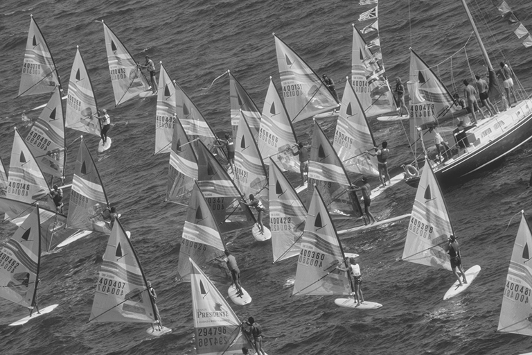
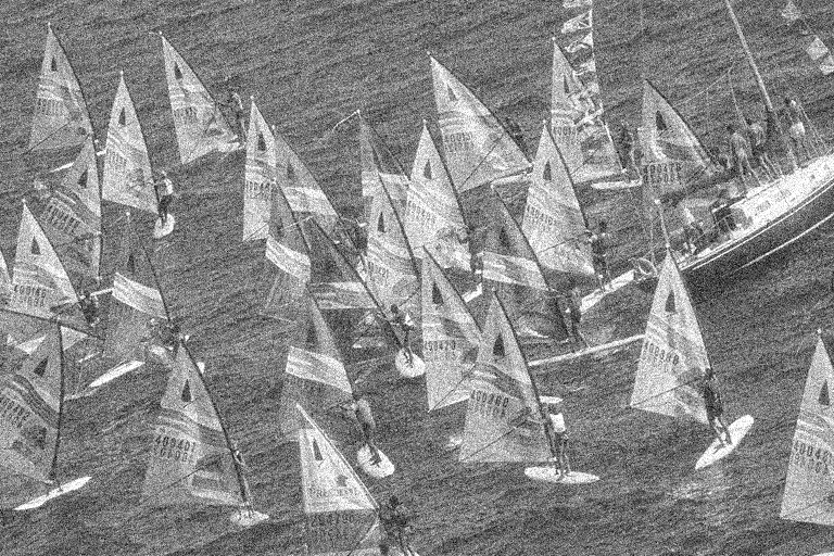
| Anisotropic TV: | Sails: | |||||||||||||||
| Res1 | Res2 | Gap | PSNR | Err | ||||||||||||
| ALM-PDP | 6(25.50s) | 1.56e-2 | 1.15e-3 | 7.31e-5 | 2.28e-5 | 1.61e-5 | 18.90 | 1e-4 | ||||||||
| ALM-PDD | 4(159.38) | 7.60e-3 | 1.97e-2 | 2.73e-4 | 2.28e-4 | 4.76e-8 | 18.90 | 1e-4 | ||||||||
| ALM-PT | 7(101.59s) | 2.72e-4 | 1.53e-2 | 1.15e-4 | 8.16e-5 | 4.55e-8 | 18.90 | 1e-4 | ||||||||
| ALG2 | 933(28.23s) | 3.35e-2 | 1.83e-3 | 2.10e-5 | 1.49e-5 | 1.08e-8 | 18.90 | 1e-4 | ||||||||
| ALM-PDP | 7(52.52s) | 5.68e-5 | 2.25e-6 | 2.03e-8 | 1.45e-8 | 9.42e-13 | 18.90 | 1e-6 | ||||||||
| ALM-PDD | 6(377.60s) | 2.18e-5 | 1.13e-5 | 9.03e-8 | 6.43e-8 | 1.25e-11 | 18.90 | 1e-6 | ||||||||
| ALM-PT | 8(337.23s) | 2.20e-5 | 5.58e-5 | 4.42e-7 | 3.17e-7 | 6.11e-11 | 18.90 | 1e-6 | ||||||||
| ALG2 | 14842(476.20s) | 3.53e-4 | 3.40e-7 | 3.94e-9 | 2.99e-9 | 3.09e-13 | 18.90 | 1e-6 | ||||||||
| ALM-PDP | 7(54.51s) | 5.65e-7 | 2.25e-6 | 2.03e-8 | 1.45e-8 | 9.38e-13 | 18.90 | 1e-8 | ||||||||
| ALM-PDD | 14(122.23s) | 2.68e-6 | 3.69e-12 | 3.44e-14 | 2.47e-14 | eps | 18.90 | 1e-8 | ||||||||
| ALM-PT | 10(363.27s) | 3.30e-6 | 1.71e-8 | 1.61e-10 | 1.14e-10 | 1.44e-14 | 18.90 | 1e-8 | ||||||||
| ALG2 | 371060(11339.88s) | 3.54e-6 | 6.98e-13 | 8.20e-15 | 5.80e-15 | eps | 18.90 | 1e-8 | ||||||||
| Isotropic TV: | Monarch: | |||||||||||||||
| Res1 | Res2 | Gap | PSNR | Err | ||||||||||||
| ALM-PDP | 3(25.12) | 1.12e-2 | 1.43e-2 | 7.31e-5 | 1.20e-4 | 4.29e-8 | 29.89 | 1e-4 | ||||||||
| ALM-PDD | 5(370.53s) | 9.89e-3 | 5.82e-3 | 3.01e-5 | 4.89e-5 | 1.54e-8 | 29.89 | 1e-4 | ||||||||
| ALM-PT | 8(2009.60s) | 8.34e-5 | 9.73e-3 | 5.13e-5 | 8.19e-5 | 2.66e-8 | 29.89 | 1e-4 | ||||||||
| ALG2 | 525(15.77s) | 2.86e-2 | 7.69e-6 | 1.02e-5 | 1.07e-3 | 4.76e-9 | 29.89 | 1e-4 | ||||||||
| ALM-PDP | 7(145.27s) | 7.98e-5 | 1.80e-4 | 9.79e-7 | 1.54e-6 | 3.15e-10 | 29.89 | 1e-6 | ||||||||
| ALM-PDD | 7(1379.33s) | 1.47e-7 | 1.09e-4 | 5.96e-7 | 9.33e-7 | 1.78e-10 | 29.89 | 1e-6 | ||||||||
| ALM-PT | — | — | — | — | — | — | — | 1e-6 | ||||||||
| ALG2 | 12049(387.21s) | 2.87e-4 | 2.61e-9 | 3.79e-9 | 4.27e-7 | 3.63e-13 | 29.89 | 1e-6 | ||||||||
| ALM-PDP | 10(1549.91s) | 1.79e-6 | 1.06e-6 | 5.90e-9 | 9.05e-9 | 8.94e-13 | 29.89 | 1e-8 | ||||||||
| ALM-PDD | — | — | — | — | — | — | — | 1e-8 | ||||||||
| ALM-PT | — | — | — | — | — | — | — | 1e-8 | ||||||||
| ALG2 | 292442(8590.28s) | 2.87e-6 | 1.56e-12 | 2.11e-12 | 2.33e-10 | eps | 29.89 | 1e-8 | ||||||||
| Isotropic TV deblurring: | Pepper: | |||||||||||||||
| Err, | Err, | |||||||||||||||
| PSNR | PSNR | |||||||||||||||
| ALM-PDP | 3(126.08s) | 1.06e-4 | 1.08e-3 | 28.48 | 3(117.37s) | 4.36e-4 | 1.07e-3 | 28.48 | ||||||||
| ALG2 | 4775(178.18s) | 2.02e-3 | 5.48e-4 | 28.36 | 4762(170.65s) | 2.02e-3 | 5.72e-4 | 28.36 | ||||||||
| Err, | Err, | |||||||||||||||
| PSNR | PSNR | |||||||||||||||
| ALM-PDP | 4(196.48s) | 3.07e-5 | 9.69e-5 | 28.48 | 4(186.79s) | 7.08e-5 | 1.70e-4 | 28.48 | ||||||||
| ALG2 | 11017(397.71s) | 2.02e-4 | 5.58e-5 | 28.47 | 10911(395.16s) | 2.02e-4 | 5.54e-5 | 28.47 | ||||||||
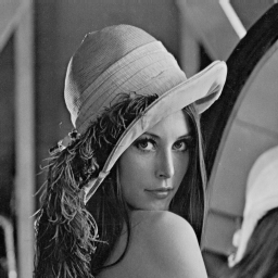
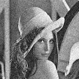
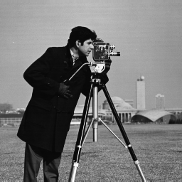
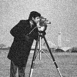
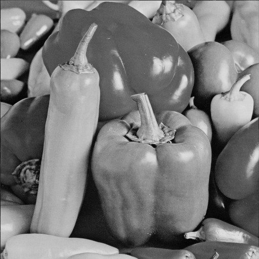
For numerical comparisons, we mainly choose the accelerated primal-dual algorithm ALG2 [4] with asymptotic convergence rate , which is very efficient, robust and standard algorithms for imaging problems. We follow the same parameters for ALG2 as in [4] and the corresponding software for the ROF model. Here we use the stopping criterion (6.1) instead of the normalized primal-dual gap (6.6) as in [4]. The test images Lena and Cameraman are with size and images Monarch and Sails are with size . The original, noisy and denoised images can be seen in Figure 1 and 2. We acknowledge that the residuals and can be unbounded without projection of to the feasible set as in ALM-PT. We leave them in the tables for references.
From Table 1 and Table 3, it can be seen that the proposed ALM-PDP, ALM-PDD and ALM-PT are very efficient and competitive for the anisotropic ROF model and are very robust for different sizes of images. From Table 2 and Table 4, it can be seen that the proposed ALM-PDP are still very efficient and competitive for the isotropic cases. The performance of ALG2 seems to hold nearly the same efficiency for the isotropic and anisotropic cases. Although the residual for smaller are much smaller for ALG2 than the proposed semismooth Newton based ALM methods, however, the residual of ALG2 is more higher than the proposed ALM methods. It seems ALG2 is more efficient for decreasing the dual error .
| res() | 3.50e-6 | 5.30e-7 | 1.53e-5 | 6.14e-8 | 3.29e-8 | 1.94e-7 |
|---|---|---|---|---|---|---|
| res() | 9.70 | 1.09 | 9.99e-2 | 6.96e-3 | 3.07e-4 | 9.13e-6 |
| Gap | 1.61e-4 | 1.41e-5 | 1.14e-6 | 5.89e-8 | 1.58e-9 | 2.58e-11 |
| 10 | 9 | 8 | 11 | 9 | 7 | |
| 20 | 29 | 51 | 56 | 102 | 116 |
Our proposed algorithms are much more efficient for the anisotropic case compared to the isotropic case for ROF denoising model. Besides Theorem 2 and 3, we present another comparison between the isotropic TV and anisotropic TV with algorithm ALM-PDP. For Table 6, we give enough Newton iterations compared to previous tables with the stopping the criterion for each ALM as in (6.10) and in (6.7) for each Newton iteration. The ALM iterations stop while Err both for the anisotropic TV.
Finally, let’s turn to the image deblurring problem. For the image deblurring with being the convolution with kernel and additional regularization term , we mainly focus on the isotropic case as in Table 5. The original, degraded and reconstructed Pepper images with size can be found in Figure 1. Since the primal model (P) is only strongly convex on the primal variable instead being strongly convex on both and , we thus employ ALG2 for comparison. The strongly convex parameter for is a subtle issue since is not invertible with the kernel. We use the strongly convex parameter of instead. It can be seen that both ALM-PDP and ALG2 are very efficient for small case. It is interesting that both ALM-PDP and ALG2 seem more efficient for the case than the case .


7 Discussion and Conclusions
In this paper, we proposed several semismooth Newton based ALM algorithms. The proposed algorithms are very efficient and competitive especially for anisotropic TV. Global convergence and the corresponding asymptotic convergence rates are also discussed with metrical subregularites. Numerical tests show that compared with first-order algorithm, more computation efforts are deserved with ALM. Currently, no preconditioners are employed by BiCGSTAB or CG for the linear systems solving Newton updated. Actually, preconditioners for BiCGSTAB or CG are desperately needed, especially for the isotropic cases. Additionally, the asymptotic convergence rate of the KKT residuals is also an interesting topic for future study [7].
Acknowledgements The author acknowledges the support of NSF of China under grant No. 11701563. The work was originated during the author’s visit to Prof. Defeng Sun of the Hong Kong Polytechnic University in October 2018. The author is very grateful to Prof. Defeng Sun for introducing the framework on semismooth Newton based ALM developed by him and his collaborators and for his suggestions on the self-adjointness of the corresponding operators for Newton updates where CG can be employed. The author is also very grateful to Prof. Kim-Chuan Toh, Dr. Chao Ding, Dr. Xudong Li and Dr. Xinyuan Zhao for the discussion on the semismooth Newton based ALM. The author is also very grateful to Prof. Michael Hintermüller for the discussion on the primal-dual semismooth Newton method during the author’s visit to Weierstrass Institute for Applied Analysis and Stochastics (WIAS) supported by Alexander von Humboldt Foundation during 2017.
References
- [1]
- [2] H. H. Bauschke, P. L. Combettes, Convex Analysis and Monotone Operator Theory in Hilbert Spaces, Springer, New York, 2011.
- [3] D. P. Bertsekas, Constrained Optimization and Lagrange Multiplier Methods, Academic Press, Paris, 1982.
- [4] A. Chambolle, T. Pock, A first-order primal-dual algorithm for convex problems with applications to imaging, J. Math. Imaging and Vis., 40(1), pp. 120–145, 2011.
- [5] F. H. Clarke, Optimization and Nonsmooth Analysis, Vol. 5, Classics in Applied Mathematics, SIAM, Philadelphia, 1990.
- [6] C. Clason, Nonsmooth Analysis and Optimization, Lecture notes, https://arxiv.org/abs/1708.04180, 2018.
- [7] Y. Cui, D. Sun, K. Toh, On the R-superlinear convergence of the KKT residues generated by the augmented Lagrangian method for convex composite conic programming, Math. Program., Ser. A, 178:38–415, 2019, https://doi.org/10.1007/s10107-018-1300-6.
- [8] T. De Luca, F. Facchinei, C. Kanzow, A semismooth equation approach to the solution of nonlinear complementarity problems, Math. Program. 75, pp. 407–439, 1996.
- [9] A. L. Dontchev, R. T. Rockafellar, Functions and Solution Mappings: A View from Variational Analysis, Second Edition, Springer Science+Business Media, New York 2014.
- [10] F. Facchinei, J. Pang, Finite-Dimensional Variational Inequalities and Complementarity Problems, Volume I, Springer-Verlag New York, Inc, 2003.
- [11] M. Fortin, R. Glowinski (eds.), Augmented Lagrangian Methods: Applications to the Solution of Boundary Value Problems, North-Holland, Amsterdam, 1983.
- [12] R. Glowinski, S. Osher, W. Yin (eds.), Splitting Methods in Communication, Imaging, Science, and Engineering, Springer, 2016.
- [13] M. R. Hestenes, Multiplier and gradient methods, J. Optim. Theory Appl., 4, pp. 303–320, 1968
- [14] M. Hintermüller, K. Kunisch, Total bounded variation regularization as a bilaterally constrained optimization problem, SIAM J. Appl. Math, 64(4), pp. 1311–1333.
- [15] M. Hintermüller, K. Papafitsoros, C. N. Rautenberg, H. Sun, Dualization and automatic distributed parameter selection of total generalized variation via bilevel optimization, preprint, to appear, 2019.
- [16] M. Hintermüller, G. Stadler, A infeasible primal-dual algorithm for total bounded variaton-based inf-convolution-type image restoration, SIAM J. Sci. Comput., 28(1), pp. 1–23, 2006.
- [17] A. J. Hoffman, On approximate solutions of systems of linear inequalities, J. Research Nat. Bur. Standards, 49 (1952), pp. 263–265.
- [18] D. Klatte, B. Kummer, Constrained minima and Lipschitzian penalties in metric spaces, SIAM J. Optim., 13(2), pp. 619–633, 2002.
- [19] D. Klatte, B. Kummer, Nonsmooth Equations in Optimization. Regularity, Calculus, Methods and Applications, Series Nonconvex Optimization and Its Applications, Vol. 60, Springer, Boston, MA, 2002.
- [20] K. Ito, K. Kunisch, Lagrange Multiplier Approach to Variational Problems and Applications, Advances in design and control 15, Philadelphia, SIAM, 2008.
- [21] K. Ito, K. Kunisch, An active set strategy based on the augmented Lagrangian formulation for image restoration, RAIRO, Math. Mod. and Num. Analysis, 33(1), pp. 1–21, 1999.
- [22] D. Leventhal, Metric subregularity and the proximal point method, J. Math. Anal. Appl., 360(2009), pp. 681-688, 2009.
- [23] R. Mifflin, Semismooth and semiconvex functions in constrained optimization, SIAM J. Control Optim., 15(6), pp. 959–972, 1977.
- [24] X. Li, D. Sun, C. Toh, A highly efficient semismooth Newton augmented Lagrangian method for solving lasso problems, SIAM J. Optim., 28(1), pp. 433–458, 2018.
- [25] F. J. Luque, Asymptotic convergence analysis of the proximal point algorithm, SIAM J. Control Optim., 22(2), pp. 277–293, 1984.
- [26] M. J. D. Powell, A method for nonlinear constraints in minimization problems, in Optimization, R. Fletcher, ed., Academic Press, New York, pp. 283–298, 1968.
- [27] M. Reed, B. Simon, Methods of Modern Mathematical Physics: Functional Analysis, Methods of Modern Math. Phys. 1, Academic Press, New York, 1980.
- [28] S. M. Robinson, Some continuity properties of polyhedral multifunctions, in Mathematical Programming at Oberwolfach, Math. Program. Stud., Springer, Berlin, Heidelberg, pp. 206–214, 1981.
- [29] R. T. Rockafellar, Monotone operators and the proximal point algorithm, SIAM J. Control Optim., 14(5), pp. 877–898, 1976.
- [30] R. T. Rockafellar, Augmented Lagrangians and applications of the proximal point algorithm in convex programming, Math. Oper. Res., 1(2), pp. 97-116, 1976.
- [31] L. I. Rudin, S. Osher, E. Fatemi, Nonlinear total variation based noise removal algorithms, Physica D., 60(1-4), pp. 259–268, 1992.
- [32] S. Scholtes, Introduction to Piecewise Differentiable Equations, Springer Briefs in Optimization, Springer, New York, 2012.
- [33] G. Stadler, Semismooth Newton and augmented Lagrangian methods for a simplified friction problem, SIAM J. Optim., 15(1), pp. 39–62, 2004.
- [34] G. Stadler, Infinite-Dimensional Semi-Smooth Newton and Augmented Lagrangian Methods for Friction and Contact Problems in Elasticity, PhD thesis, University of Graz, 2004.
- [35] D. Sun and J. Han, Newton and quasi-Newton methods for a class of nonsmooth equations and related problems, SIAM J. Optim., 7, pp. 463–480, 1997.
- [36] M. Ulbrich, Semismooth Newton Methods for Variational Inequalities and Constrained Optimization Problems in Function Spaces, MOS-SIAM Series on Optimization, 2011.
- [37] H. A. Van der Vorst, Iterative Krylov Methods for Large Linear Systems, Cambridge University Press, Cambridge, 2003.
- [38] J. Ye, X. Yuan, S. Zeng, J. Zhang, Variational analysis perspective on linear convergence of some first order methods for nonsmooth convex optimization problems, Set-Valued Var. Anal., https://doi.org/10.1007/s11228-021-00591-3, 2021.
- [39] P. Yu, G. Li, TK. Pong, Deducing Kurdyka-Lojasiewicz exponent via inf-projection, Found. Comput. Math., https://doi.org/10.1007/s10208-021-09528-6, 2021.
- [40] F. Zhang (eds.), The Schur Complement and Its Applications, Numerical Methods and Algorithms 4, Springer US, 2005.
- [41] Y. Zhang, N. Zhang, D. Sun, K. Toh, An efficient Hessian based algorithm for solving large-scale sparse group Lasso problems, Mathematical Programming A, https://doi.org/10.1007/s10107-018-1329-6, 2018.
- [42] X. Zhao, D. Sun, K. Toh, A Newton-CG augmented Lagrangian method for semidefinite programming, SIAM J. Optim., 20(4), pp. 1737–1765, 2010.