Periodic orbits of active particles induced by hydrodynamic monopoles

Abstract

Terrestrial experiments on active particles, such as Volvox, involve gravitational forces, torques and accompanying monopolar fluid flows. Taking these into account, we analyse the dynamics of a pair of self-propelling, self-spinning active particles between widely separated parallel planes. Neglecting flow reflected by the planes, the dynamics of orientation and horizontal separation is symplectic, with a Hamiltonian exactly determining limit cycle oscillations. Near the bottom plane, gravitational torque damps and reflected flow excites this oscillator, sustaining a second limit cycle that can be perturbatively related to the first. Our work provides a theory for dancing Volvox and highlights the importance of monopolar flow in active matter.

Since Lighthill’s seminal work on the squirming motion of a sphere (Lighthill, 1952; Blake, 1971a), it has been understood that freely moving active particles produce hydrodynamic flows that disallow monopoles and antisymmetric dipoles (Anderson, 1989). The minimal representation of active flows by the symmetric dipole, the leading term consistent with force-free, torque free-motion, has been the basis of much theoretical work in both particle (Lauga and Powers, 2009; Drescher et al., 2010; Koch and Subramanian, 2011) and field representations of active matter (Marchetti et al., 2013; Ramaswamy, 2017). The importance of multipoles beyond leading order in representing experimentally measured flows around active particles has now been recognized and their effects have been included in recent theoretical work (Ghose and Adhikari, 2014; Pedley et al., 2016). Less recognised, however, is the fact that active particles in typical experiments (Drescher et al., 2009, 2010; Goldstein, 2015; Palacci et al., 2013, 2010; Buttinoni et al., 2013; Ebbens and Howse, 2010) are neither force- nor torque-free: mismatches between particle and solvent densities lead to net gravitational forces while mismatches between the gravitational and geometric centers lead to net gravitational torques. In this case, both monopolar and antisymmetric dipolar flows are allowed and become dominant, at long distances, over active contributions. It is of great interest, therefore, to understand how these components influence the dynamics of active particles and, more generally, of active matter.

Theoretical work on this aspect of active matter has been limited, even though the effect of monopolar flow in passive, driven matter is well-understood (Smoluchowski, 1911; Brenner, 1963; Ladd, 1988; Squires and Brenner, 2000; Squires, 2001). Attraction induced by monopolar flow near boundaries has been shown to cause crystallisation of active particles (Singh and Adhikari, 2016). Reorientation induced by monopolar vorticity has been identified as the key mechanism in the emergence of the pumping state of harmonically confined active particles (Nash et al., 2010; Singh et al., 2015). However, none of these studies have focused on the dynamics of pairs, which forms the foundation for understanding collective motion, or attempted an analytical description of motion.

In this Letter, we provide a theory for the dynamics of density-mismatched, bottom-heavy, self-propelling and self-spinning active particles between widely separated parallel planes. Starting from the ten-dimensional equations for hydrodynamically interacting active motion in the presence of external forces and torques, we derive, by exploiting symmetries, a lower-dimensional dynamical system for the pair. For positive buoyant mass, negative gravitaxis, and negligible reflected flow, we obtain a sedimenting state with limit cycle oscillations in the relative orientation and horizontal separation. The dynamics is symplectic and a Hamiltonian completely determines the properties of periodic orbits. On approach to the bottom wall, reflected flow arrests sedimentation and yields a levitating state with limit cycle oscillations that now includes the mean height. This second limit cycle can be understood as a damped (by gravitational torque) and driven (by reflected flow) perturbation of the first. These rationalise the Volvox dance (Drescher et al., 2009; Goldstein, 2015) and highlight the importance of monopolar hydrodynamic flow in active matter. We now explain how our results are obtained.

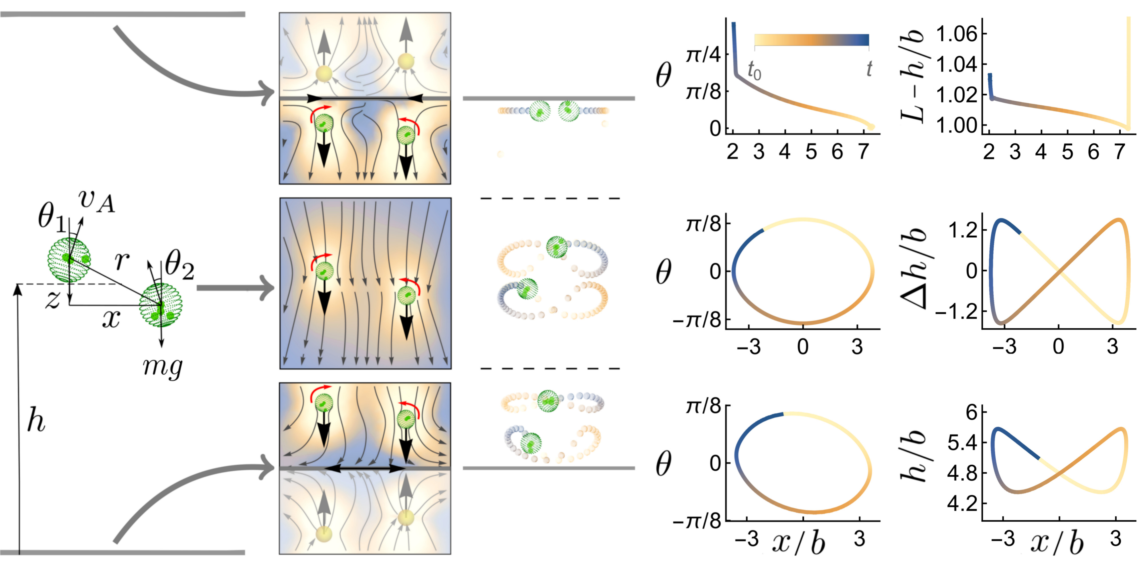
Figure 1: Fixed point and limit cycles of the five-dimensional dynamics system of Eq.(2-3). First column: coordinate system used to describe a pair of particles between two parallel plane surfaces. Second column: streamlines of the monopolar flow (red curved arrows show flow-induced rotations of the particles) superimposed on a pseudo colormap of the flow speed. The plots correspond to the following three cases: top row: near the top surface, middle row: away from the surfaces, and bottom row: near the bottom surface. Third column: stroboscopic images of the two-particle dynamics in the three configurations. The dynamical system admits a fixed point at the top surface, while limit cycles are formed away from the surfaces and near the bottom surface. The last two columns contain the plot of relative orientation $\theta$ and average height $h$ as a function of $x$ for the three cases. The colorbar indicates time in the final 3 columns and $L$ is the separation of the planes. See movie 1 of SI.

Full and reduced equations: We consider a pair of spherical active particles of radius $b$, density $\rho$, self-propulsion speed $v_{A}$, and self-rotation speed $\omega_{A}$, in an incompressible Newtonian fluid of density $\rho_{f}$ and viscosity $\eta$ between parallel planes whose separation is $L\gg b$ (greenFuncApprox, ). Their geometric centres, propulsive orientations, velocities, and angular velocities are, respectively, $\boldsymbol{R}_{i}$, $\boldsymbol{p}_{i}$, $\boldsymbol{V}_{i}$ and $\boldsymbol{\Omega}_{i}$, where $i=1,2$ is the particle index. Overdamped, hydrodynamically interacting, active motion in the presence of body forces $\boldsymbol{F}_{j}^{B}$ and body torques $\boldsymbol{T}_{j}^{B}$ is given by (Singh and Adhikari, 2018)

$$\boldsymbol{V}_{i}=\boldsymbol{\mu}_{ij}^{TT}\cdot\boldsymbol{F}_{j}^{B} +\boldsymbol{\mu}_{ij}^{TR}\cdot\boldsymbol{T}_{j}^{B}+v_{A}\boldsymbol{p}_{i},$$ (1)

$$\boldsymbol{\Omega}_{i}=\boldsymbol{\mu}_{ij}^{RT}\cdot\boldsymbol{F}_{j}^{B} +\boldsymbol{\mu}_{ij}^{RR}\cdot\boldsymbol{T}_{j}^{B}+\omega_{A}\boldsymbol{p}_{i}$$

where $\boldsymbol{\mu}_{ij}^{\alpha\beta}$ are mobility matrices and repeated particle indices are summed. Positions and orientations obey the kinematic equations $\dot{\boldsymbol{R}}_{i}=\mathbf{V}_{i},$ and $\dot{\boldsymbol{p}}_{i}=\mathbf{\boldsymbol{\Omega}}_{i}\times\boldsymbol{p}_{i}$. The above follow directly from Newton’s laws for active particles when inertia and active flows are neglected (siT, ). The expression for the exterior fluid flow $\boldsymbol{v}(\boldsymbol{r})$ around the colloids is then: $\boldsymbol{v}(\boldsymbol{r})=(1+\tfrac{b^{2}}{6}\nabla^{2})\,\mathbf{G}\cdot\boldsymbol{F}_{i}^{B}+\frac{1}{2}(\boldsymbol{\nabla}\times\mathbf{G})\cdot\boldsymbol{T}_{i}^{B}$, where $\mathbf{G}$ is a Green’s function of Stokes equation (Pozrikidis, 1992) which satisfies the appropriate boundary conditions at the boundaries in the flow. The flow due to self-propulsion and self-spin involve, respectively, two and three gradients of the Green’s function and are thus subdominant (Ghose and Adhikari, 2014; Singh and Adhikari, 2018). For a sphere in a gravitational field $\boldsymbol{g}$, the force is $\boldsymbol{F}_{i}^{B}$=$m\boldsymbol{g}$, where $m$=$\frac{4\pi b^{3}}{3}$$(\rho-\rho_{f})$ is the buoyant mass and the torque is $\boldsymbol{T}_{i}^{B}$=$\boldsymbol{d}_{i}\times(\frac{4\pi b^{3}}{3}\rho\boldsymbol{g})$, where $\boldsymbol{d}_{i}$ is the position of the centre of gravity relative to $\boldsymbol{R}_{i}$ (Pedley and Kessler, 1992). The torque aligns $\boldsymbol{d}_{i}$ parallel to $\boldsymbol{g}$ and positive/negative gravitaxis results when $\boldsymbol{p}_{i}$ is parallel/anti-parallel to $\boldsymbol{d}_{i}$. Typical estimates of these parameters for a $Volvox$ are $b\sim 300$$\mathrm{\mu m}$, $v_{A}\sim 300$$\mathrm{\mu m/s}$, $mg\sim 1\mathrm{nN}$, $\omega_{A}\sim 1$ rad/s (Drescher et al., 2009). Thus, the typical active forces $F^{A}\sim 6\pi\eta bv_{A}\sim 10^{-9}$N and torques $T^{A}\sim 8\pi\eta b^{3}\omega^{A}\sim 10^{-12}$Nm. Thus, Brownian forces $k_{B}T/b\sim 10^{-14}$N and torques $k_{B}T\sim 10^{-20}$Nm can be neglected for such systems of active particles. We now present a reduced description of our deterministic equations of motion.

Our dimensional reduction is motivated by a symmetry of Stokes flow that constrains motion initially in a plane perpendicular to the torque to remain in that plane. We choose $y=0$ to be the plane of motion, set $\boldsymbol{F}_{i}^{B}=-mg\hat{\boldsymbol{z}}$, $\boldsymbol{T}_{i}^{B}=T_{R}\boldsymbol{p}_{i}\times\hat{\boldsymbol{z}}$, where $T_{R}=\frac{4\pi b^{3}}{3}\rho gd$ is the magnitude of the gravitational torque, and parametrise $\boldsymbol{R}_{i}=x_{i}\hat{\boldsymbol{x}}+z_{i}\hat{\boldsymbol{z}}$ and $\boldsymbol{p}_{i}=\sin\theta_{i}\hat{\boldsymbol{x}}+\cos\theta_{i}\hat{\boldsymbol{z}}$, so that $\boldsymbol{V}_{i}=\dot{x}_{i}\hat{\boldsymbol{x}}+\dot{z}_{i}\hat{\boldsymbol{z}},$ and $\boldsymbol{\Omega}_{i}=\dot{\theta}_{i}\hat{\boldsymbol{y}}$. Using these and translational and time-reversal symmetries in Eq.(1), retaining terms in the mobility matrices to leading order in $x_{1}-x_{2}$, $z_{1}$ and $z_{2}$, discarding the decoupled equation for the horizontal component of the center of mass, and expressing the result in terms of the reduced variables $2\dot{\psi}=\dot{\theta}_{1}+\dot{\theta}_{2}$, $2\dot{\theta}=\dot{\theta}_{1}-\dot{\theta}_{2}$, $x=x_{1}-x_{2},$ $z=z_{1}-z_{2}$, $2h=z_{1}+z_{2}$, we obtain a five-dimensional dynamical system (siT, ), partitioned into two orientational equations

$$\dot{\psi} =\mkern-3.0mu-\frac{T_{R}}{8\pi\eta b^{3}}\sin\psi\cos\theta,$$ (2a)

$$\dot{\theta} =\mkern-3.0mu-\frac{T_{R}}{8\pi\eta b^{3}}\cos\psi\sin\theta-\frac{mg}{8\pi\eta}\left[\frac{x}{r^{3}}\mkern-3.0mu-\mkern-4.0mu\frac{x}{(4h^{2}\mkern-3.0mu+\mkern-3.0mur^{2})^{3/2}}\right]$$ (2b)

and three positional equations,

$$\dot{x} =\,\,\,\,2v_{A}\cos\psi\sin\theta+\frac{mghx}{2\pi\eta(4h^{2}+r^{2})^{3/2}},$$ (3a)

$$\dot{z} =-2v_{A}\sin\psi\cos\theta-\frac{mgz}{2\pi\eta(4h^{2}-z^{2})},$$ (3b)

$$\dot{h} =v_{A}\cos\psi\cos\theta-\frac{mg}{8\pi\eta}\left(\frac{4}{3b}+\frac{1}{r}+\frac{z^{2}}{r^{3}}-\frac{2}{h}\right).$$ (3c)

The geometry of the reduced variables is shown in Fig. (1). The orientational equations describe the competition between gravitational torques that restore vertical orientations (noteStability, ) and hydrodynamic torques, from monopolar vorticity, that promotes relative re-orientation. The first and second positional equations describe the change in relative separation due to gravitaxis and reflected monopolar flow, the latter of which increases horizontal separation and decreases vertical separation (Squires, 2001). The third positional equation describes the competition between the tendency of the mean height to increase, due to gravitaxis and reflected monopolar flow, and its tendency to decrease, due to gravitational forces and monopolar flow. Eqs.(2-3) describe the sedimentation of a pair of passive particles when $v_{A},\omega_{A}=0$ (Smoluchowski, 1911); the horizontal dynamics of a pair of phoretic particles when $v_{A}\neq 0,\omega_{A}=0$ and both the height and orientation are fixed (Squires, 2001); and the coupled dynamics of horizontal separation and relative orientation when $v_{A}\neq 0,\omega_{A}\neq 0$ and the height is fixed (Drescher et al., 2009).

Hamiltonian limit cycle: We now analyse Eqs.(2-3), initially neglecting the reflected flow. We assume initial heights that are remote from both planes, $0\ll z_{1},z_{2}\ll L$ and parameter values, to be identified below, that ensure sedimentation in the mean. The attractor $\psi=0$ of the first orientational equation, reached on the time scale $\omega_{R}=T_{R}/8\pi\eta b^{3}$, defines the slow manifold $\theta_{1}+\theta_{2}=0$. On this slow manifold and neglecting reflected flow, reorientation is principally due to the monopolar vorticity, $\dot{\theta}=-mgx/8\pi\eta r^{3}$, relative horizontal motion is principally due to gravitaxis, $\dot{x}=2v_{A}\sin\theta$, and relative vertical motion is absent, $\dot{z}=0.$ Remarkably, the dynamics, which are governed by the reduced equations (2b,3a,3c), has the symplectic form $\dot{x}=-\partial_{\theta}H$, $\dot{\theta}=\partial_{x}H$ with Hamiltonian

$$H(x,\theta)=\frac{mg}{8\pi\eta}\frac{1}{\sqrt{x^{2}+z^{2}}}+2v_{A}\cos\theta$$ (4)

which has the dimension of velocity and is a constant of motion (divfreeH, ). Position and angle are canonically conjugate variables and the dynamics preserves the two- form $dx\wedge d\theta$ (Arnold, 2013). Level sets $H(x,\theta)=E$ of the Hamiltonian, shown in Fig.(2a), define orbits in the $x-\theta$ plane labelled by the “energy” $E$. For closed orbits, $\theta$ vanishes at the turning points and $x$ reaches its maximum $x_{m}$, giving $E=mg/8\pi\eta\sqrt{x_{m}^{2}+z^{2}}+2v_{A}\geq 2v_{A}$ as a bound for such orbits. Trajectories on the orbit are obtained by integrating $dt=-dx/\partial_{\theta}H=d\theta/\partial_{x}H$ at constant energy, from which the period follows directly. For small oscillations, a quadratic approximation to the Hamiltonian shows that $x$ and $\theta$ vary harmonically with frequency $\omega_{0}=2\pi/T_{0}=\sqrt{mgv_{A}/\eta z^{3}}$. For large oscillations, the trajectory integrals can be obtained exactly in terms of elliptic functions (Gradshteyn and Ryzhik, 2014). The result for the period $T_{E}$, scaled by the frequency of small oscillations, is shown in Fig.(2b). The mean height is driven by the Hamiltonian limit cycle and its change per period is

$$\frac{\Delta h}{T_{E}}=-\left(v_{0}+E\right)+\langle 3v_{A}\cos\theta-v_{0}\frac{3bz^{2}}{4r^{3}}\rangle$$ (5)

where angled brackets denote orbital averages at energy $E$ and $v_{0}=\frac{mg}{6\pi\eta b}$. The right hand side averages can be obtained exactly in terms of elliptic functions (Gradshteyn and Ryzhik, 2014). The mean sedimentation speed $\Delta h/T_{E}$ thus obtained is shown in Fig.(2c). The root of the above equation determines the critical value $E_{0}$ of the energy above (below) which the net vertical motion is upward (downward). A typical sedimenting trajectory, $E>E_{0}$, is shown in $x-\theta-h$ space in Fig.(2d).

The symplectic structure is destroyed when the re-orienting effect of the gravitational torque is included. The Hamiltonian increases monotonically at the rate $\dot{H}=T_{R}v_{A}\sin^{2}\theta/4\pi\eta b^{3}$ to its maximum value of $mg/8\pi\eta z+2v_{A}$ at $x=\theta=0$, and this corresponds to the pair sedimenting with a vertical separation $z$ and oriented vertically. We next examine how reflected flow alters these exact results.

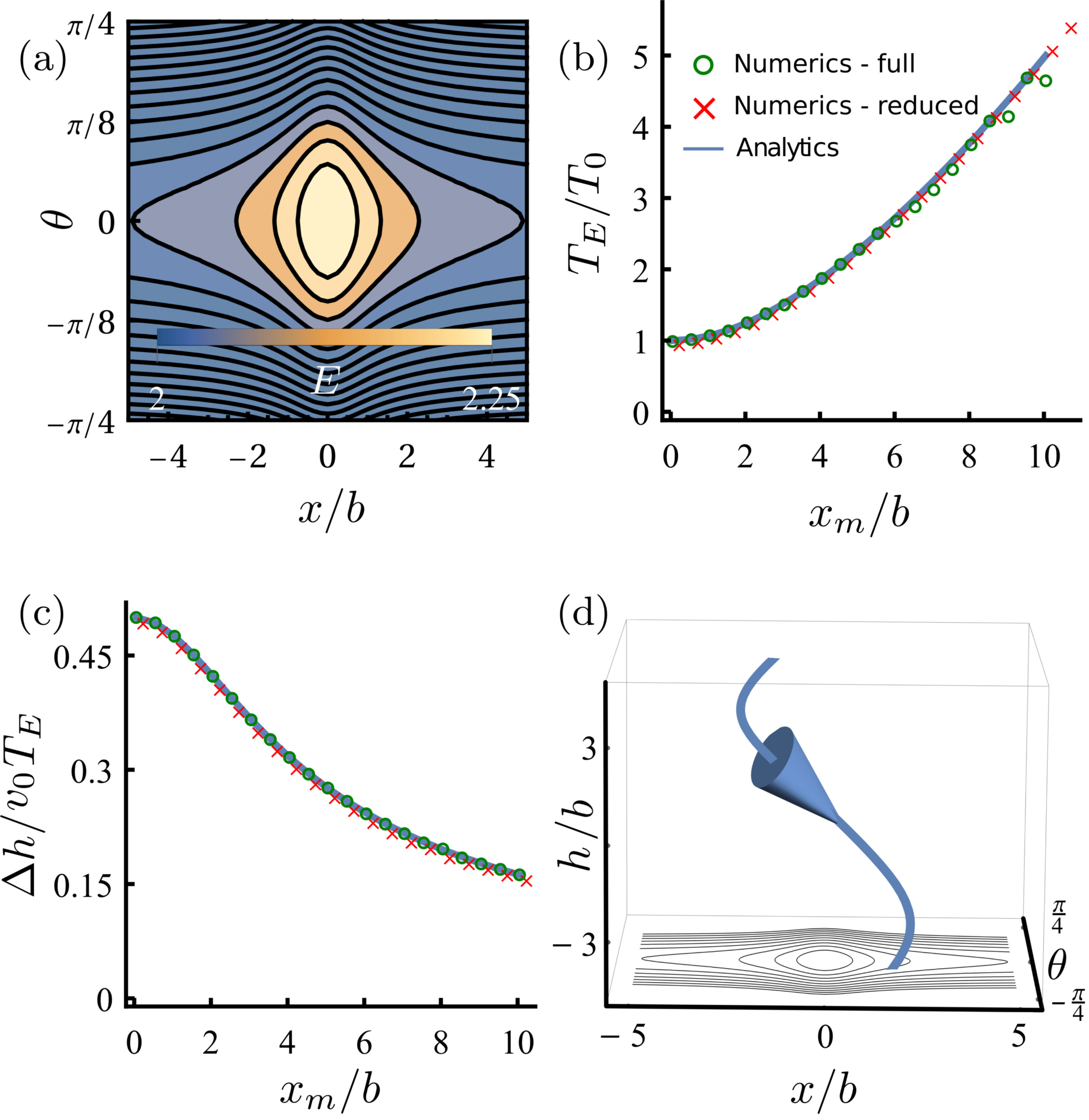
Figure 2: Exact solution of the Hamiltonian limit cycle. (a) level sets of the Hamiltonian in which the reflection symmetries $x\rightarrow-x$ and $\theta\rightarrow-\theta$ are clearly visible, (b) variation of the period of large oscillations $T_{E}$ as a function of their amplitude scaled by the period of small oscillations. Using experimental values (Drescher et al., 2009), we obtain $T_{0}\sim 8$s giving $T_{E}\sim 12$s for $x_{m}=z=3$. This agrees well with the experimentally measured time period of the “minuet” bound state (Drescher et al., 2009), (c) sedimentation speed as a function of the oscillation amplitude, and (d) orbit on a constant “energy” manifold in $x,\theta$ and $h$ with the level sets of $H$ shown on a cross-section. Exact analytical results are compared with numerical simulations of the full (Eq.(1)) and reduced (Eqs.(2b,3a,3c))

equations in (b) and (c) with $T_{R},\,1/h=0$.

Limit cycle near bottom plane: The effect of reflected flow appears at different orders of $h$ in the dynamical system. In decreasing order of importance, $h$ dynamics receive an $O(b/h)$ reduction in the effective mobility, $z$ dynamics receive an $O(b^{2}/h^{2})$ hydrodynamic attraction, $x$ dynamics receive an $O(b^{2}/h^{2})$ hydrodynamic repulsion, and $\theta$ dynamics receive an $O(b^{3}/h^{3})$ contribution to reorientation. A levitating state at a mean height $h^{\star}$ can exist if the change in mean height per period is zero, giving

$$-\left(v_{0}+E\right)+\langle 3v_{A}\cos\theta-v_{0}\left(\frac{3bz^{2}}{4r^{3}}-\frac{3b}{2h}\right)\rangle=0.$$ (6)

The rate of change of the Hamiltonian on the true limit cycle is $\dot{H}=T_{R}v_{A}\sin^{2}\theta/4\pi\eta b^{3}-\left(\frac{mg}{8\pi\eta}\right)^{2}\frac{x^{2}}{2\left(x^{2}+z^{2}\right)^{3/2}h^{2}}$ and, if this is to vanish over an orbit, we must have

$$\langle\dot{H}\rangle=\langle 2\omega_{R}v_{A}\sin^{2}\theta-\frac{9b^{2}v_{0}^{2}x^{2}}{32\left(x^{2}+z^{2}\right)^{3/2}h^{2}}\rangle=0.$$ (7)

To $O(z^{3}/h^{3})$ the average over the true limit cycle can be replaced by an average over the Hamiltonian limit cycle at some energy $E^{\star}$ (Krylov and Bogoli︠u︡bov, 1947). The above pair of equations, in which averages are taken over Hamiltonian orbits, implicitly determines unique values of $h^{\star}$ and $E^{\star}$ which define the levitating, periodic, stable limit cycle in the presence of reflected flow (see Fig.(3)). Unlike (Drescher et al., 2009), we do not find a Hopf bifurcation but rather a transient decay of the Hamiltonian limit cycle into a stable one (noteDrescher, ).

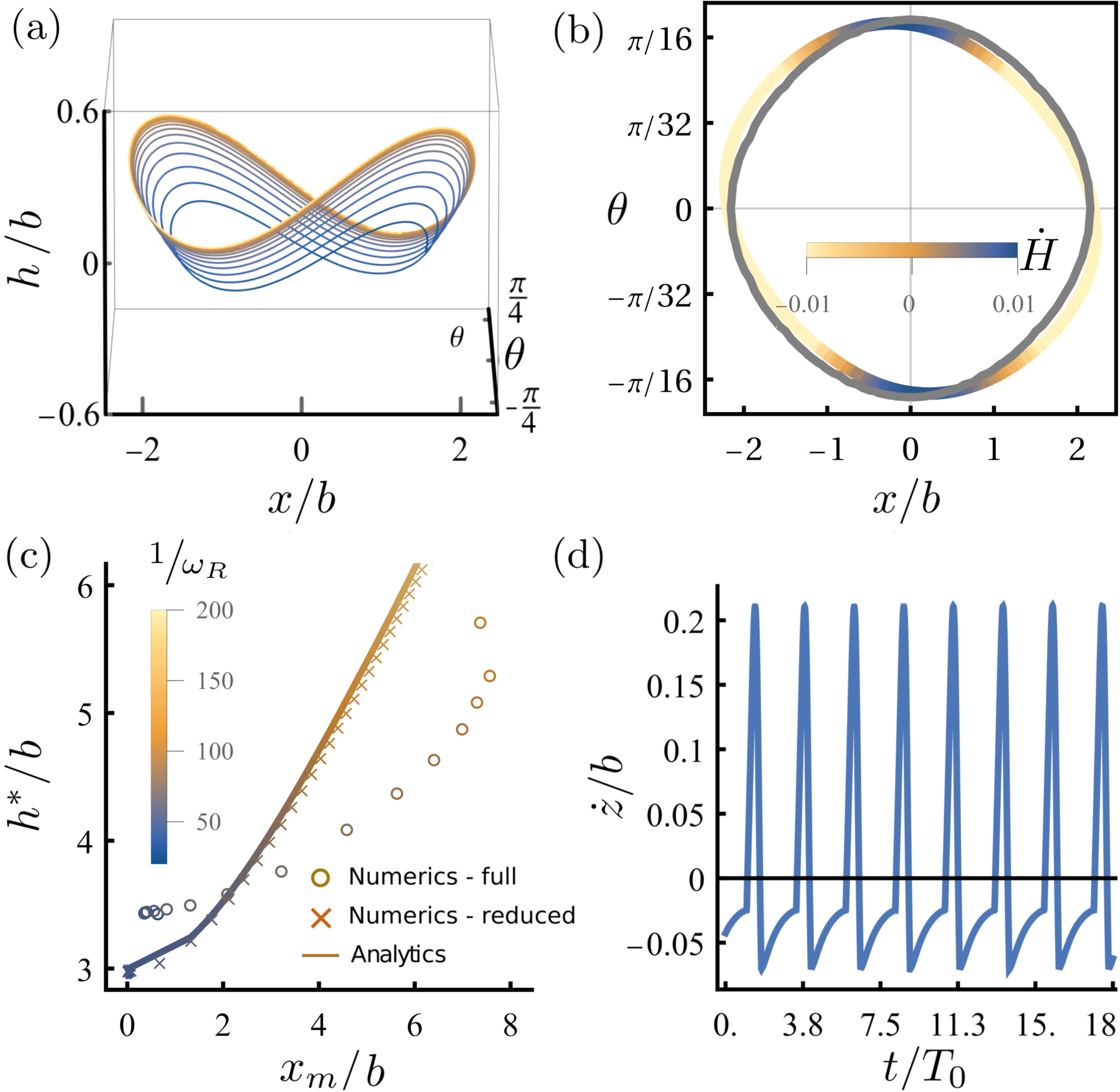
Figure 3: Perturbative solution of the two-body system near the bottom plane, (a) a stable limit cycle is formed in the presence of the bottom plane at height $h^{\star}$ and “energy” $E^{\star}$, (b) an overlay of the numeric and analytic contours with $E=2.2$. The colormap shows instantaneous “power” input into the numerical limit cycle from perturbative effects which produce small deformations to the shape of the orbit, (c) the period averaged levitation height from the bottom plane $h^{\star}/b$ against the maximum amplitude $x_{m}$ for the limit cycle as $\omega_{R}$ is varied. Excellent quantitative agreement between the analytic solution in Eqs.(6-7) and the reduced numerics justifies, a posteriori, averaging over the Hamiltonian orbit. Qualitative agreement between analytics and the full equations of motion shows the monotonic increase of $h^{\star}$ with $E^{\star}$ survives when the complete dynamics is considered. A fixed value of $z/b=2$ was used for analytic and reduced numerical computations while a more realistic short-ranged repulsive harmonic potential was implemented in the full numerics, resulting in a non-zero $\dot{z}$. (d) the spikes in $\dot{z}/b$ are caused by steric repulsion induced by the short-ranged potential. Thus, over an oscillation, the value of $z$ changes, leading to quantitative disagreement as seen in (c).

Fixed point at top plane: For energy values $E<E_{0}$ the net vertical motion is upwards. In this case, the dynamical system must be modified to account for the proximity of the top plane. This is obtained by replacing $h$ by $\pm(L-h)$ in Eqs.(2-3). The effect of reflected flow from the top surface is now the reverse and instead of being destabilising is stabilising. The limit cycle is destroyed and, instead, a dimerised state is obtained due to the attractive flow of the monopoles pointing away from the plane (Squires and Brenner, 2000). This is identical in mechanism but distinct in detail to flow-induced phase separation of active particles which swim into the plane surface (Singh and Adhikari, 2016).

Conclusion: We have presented overdamped equations for the hydrodynamically interacting dynamics of a pair of self-propelling, self-spinning particles in the presence of external forces and torques confined between planes. We have identified a regime away from both planes where the dynamics is symplectic, with a Hamiltonian determing periodic orbits. A second regime near the bottom plane has a limit cycle which can be related perturbatively to the Hamiltonian oscillator. A third regime at the top plane is non-periodic with a fixed point. Qualitatively, the reflection of the monopolar flow at the top/bottom plane approximates extensile/contractile dipolar flow (Squires and Brenner, 2000) and destablises/stabilises the Hamiltonian limit cycle. A simple criterion has been found for bifurcations between these states, determined by the value of Hamiltonian $E$. Notably, this mechanism is operative at both no-slip and no-shear planes as it appears at leading order in the reflection; next-to-leading order terms only alter the time-scales of motion (sec IV of SI (siT, )). Our theory can be extended to many-particle levitating states of active matter, such as active emulsion droplets, by including next to leading order effects from symmetric dipoles and will be presented elsewhere ($Al.$, ). Our work shows that active matter, which breaks time-reversal invariance (Fodor et al., 2016) and is inherently dissipative (Singh and Adhikari, 2018), may nonetheless be described by Hamiltonian dynamics.

Acknowledgements: We acknowledge the EPSRC (AB), the Royal Society-SERB Newton International Fellowship (RS) and the Isaac Newton Trust (RA) for support. We thank Prof. M. E. Cates for critical remarks and Prof. R. E. Goldstein for helpful discussions and for bringing (Squires and Brenner, 2000) to our attention.We note that, since submission of this manuscript, a detailed state-of-the-art boundary element analysis of a pair of Volvox has appeared in (Ishikawa et al., 2020).

Supplemental Information (SI)

I full equations of motion and numerical solution

We consider a system of active colloids labeled as $i=1,\dots N$ of radius $b$ in an incompressible fluid of viscosity $\eta$. The centre of mass of the $i$th colloid is denoted by $\boldsymbol{R}_{i}$, while a unit vector $\boldsymbol{p}_{i}$ denotes its orientation. The translational $\boldsymbol{V}_{i}$ and rotational velocity $\boldsymbol{\Omega}_{i}$ is given from the sum of all the forces and torques acting on the colloids

$$m\boldsymbol{\dot{V}}_{i}=-\boldsymbol{\gamma}_{ij}^{TT}\cdot(\boldsymbol{V}_{j}-v_{A}\boldsymbol{p}_{j})-\boldsymbol{\gamma}_{ij}^{TR}\cdot(\boldsymbol{\Omega}_{j}-\omega_{A}\boldsymbol{p}_{j})+\boldsymbol{F}_{i}^{B} =0$$

$$I\boldsymbol{\dot{\Omega}}_{i}\boldsymbol{=}-\boldsymbol{\gamma}_{ij}^{RT}\cdot(\boldsymbol{V}_{j}-v_{A}\boldsymbol{p}_{j})-\boldsymbol{\gamma}_{ij}^{RR}\cdot(\boldsymbol{\Omega}_{j}-\omega_{A}\boldsymbol{p}_{j})+\boldsymbol{T}_{i}^{B} =0$$

Here $v_{A}$ (and $\omega_{A}$) is the self-propulsion translational (rotational) speed of an isolated colloid, $\boldsymbol{\gamma}^{\alpha\beta}$, for $(\alpha,\beta=T,R)$, are friction tensors (Ladd, 1988), while $\boldsymbol{F}_{i}^{B}$ and $\boldsymbol{T}_{i}^{B}$ are the body forces and torques on the $i$th colloid.

In the microhydrodynamic regime, as applicable to colloidal scale, the inertia can be ignored, and the rigid body motion is then given as(Ladd, 1988; Singh and Adhikari, 2018)

$$\boldsymbol{V}_{i}=\boldsymbol{\mu}_{ij}^{TT}\cdot\boldsymbol{F}_{j}^{B} +\boldsymbol{\mu}_{ij}^{TR}\cdot\boldsymbol{T}_{j}^{B}+v_{A}\boldsymbol{p}_{i}$$

$$\boldsymbol{\Omega}_{i}=\boldsymbol{\mu}_{ij}^{RT}\cdot\boldsymbol{F}_{j}^{B} +\boldsymbol{\mu}_{ij}^{RR}\cdot\boldsymbol{T}_{j}^{B}+\omega_{A}\boldsymbol{p}_{i}$$

Here $\boldsymbol{\mu}^{\alpha\beta}$, for $(\alpha,\beta=T,R)$, are the mobility matrices (Ladd, 1988).

The above equations have been simulated using PyStokes, a python package for simulating Stokesian hydrodynamics (R. Singh and Adhikari, 2019). The initial parameters were set to $b=1,\,v_{A}=1,\,v_{0}=1$. We then study the system near a plane surface by computing the mobility tensors using the appropriate Green’s function of Stokes equation which satisfies the boundary conditions of no-slip (Blake, 1971b) or no-shear (Aderogba and Blake, 1978) at a plane surface. Our system of active particles near a plane surface has no periodic boundary condition and the particles are allowed to explore the infinite half-space around the surface. For simulations near the bottom plane, an additional restoring torque of strength $\omega_{R}=0.022$ was added due to bottom-heaviness of the colloids. In this case, $z$ becomes a dynamic variable and the separation changes greatly over the time period of a cycle. In order to prevent the active particles getting too close to one another an additional soft harmonic repulsion of strength $2$ was introduced when the particles came within $6.3$ units of radius $b$ of one another. This kept the particles separated by an average vertical distance $z=3$ during integration allowing comparison to be made with the analytics and numerics of the reduced equations. Making this potential soft and longer ranged made numerical integration more stable and allowed larger integrator step sizes to be taken which reduced the cost of running longer simulations. It was not necessary to include a repulsive contact potential from the surface as the particles were at least a distance $b$ away due to hydrodynamic repulsion from the image charges. A two-particle simulation of above equation leads to the formation of time-dependent bound state as described in the main text. See Fig.(4) for snapshots from the dynamics.

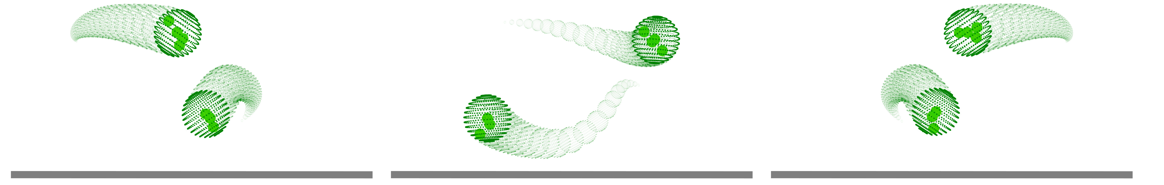
Figure 4: Stroboscopic images from the dynamics of two active particles near a plane no-shear surface. A similar dynamics is also obtained near a plane no-slip surface but with a longer time scale due to reduced strength of the hydrodynamic interactions.

For simulations near the top surface, the same values were used.

	$\boldsymbol{\mu}_{ij}^{TT}=(1+\frac{b^{2}}{3}\nabla^{2})\mathbf{G}$	$\boldsymbol{\mu}_{ij}^{TR}=\frac{1}{2}\boldsymbol{\nabla}_{{\scriptscriptstyle\boldsymbol{R}_{j}}}\times\mathbf{G}$	$\boldsymbol{\mu}_{ij}^{RR}=\frac{1}{4}\boldsymbol{\nabla}_{{\scriptscriptstyle\boldsymbol{R}_{i}}}\times\boldsymbol{\nabla}_{{\scriptscriptstyle\boldsymbol{R}_{j}}}\times\mathbf{G}$
Bottom
plane	$\mu_{ii}^{zz}=\frac{1}{6\pi\eta b}\Big{(}1-\frac{3b}{4z_{i}}\Big{)}$.	$\tilde{\mu}_{ii}^{zy}=0$	$\hat{\mu}_{ii}^{yy}=\frac{1}{8\pi\eta b^{3}}\Big{(}1-\frac{1}{16}\frac{b^{3}}{z_{i}^{3}}\Big{)}$
Bottom
plane	$\mu_{12}^{xz}=\frac{1}{8\pi\eta}\bigg{[}\frac{(x_{1}-x_{2})(z_{1}-z_{2})}{r^{3}}-\frac{(x_{1}-x_{2})(z_{1}+z_{2})}{r^{{}^{*}3}}\bigg{]}$	$\tilde{\mu}_{12}^{xy}=\frac{1}{8\pi\eta}\bigg{[}\frac{(z_{1}-z_{2})}{r^{3}}-\frac{(z_{1}+z_{2})}{r^{{}^{*}3}}\bigg{]}$	$\hat{\mu}_{12}^{yy}=-\frac{1}{16\pi\eta}\bigg{[}\frac{1}{r^{3}}-\frac{3(y_{1}-y_{2})(y_{1}-y_{2})}{r^{5}}+\frac{1}{r^{*3}}-\frac{3(y_{1}-y_{2})(y_{1}-y_{2})}{r^{{}^{*}5}}\bigg{]}$
Bottom
plane	$\mu_{12}^{zz}=\frac{1}{8\pi\eta}\bigg{[}\frac{1}{r}+\frac{(z_{1}-z_{2})(z_{1}-z_{2})}{r^{3}}-\frac{1}{r^{*}}-\frac{(z_{1}+z_{2})(z_{1}+z_{2})}{r^{{}^{*}3}}\bigg{]}$	$\tilde{\mu}_{12}^{yz}=\frac{1}{8\pi\eta}\bigg{[}\frac{(x_{1}-x_{2})}{r^{3}}-\frac{(x_{1}-x_{2})}{r^{{}^{*}3}}\bigg{]}$	$\hat{\mu}_{12}^{zy}=-\frac{1}{16\pi\eta}\bigg{[}\frac{1}{r^{3}}+\frac{3(y_{1}-y_{2})(z_{1}-z_{2})}{r^{5}}-\frac{1}{r^{*3}}-\frac{3(y_{1}-y_{2})(z_{1}+z_{2})}{r^{{}^{*}5}}\bigg{]}$
Top
plane	$\mu_{ii}^{zz}=\frac{1}{6\pi\eta b}\Big{(}1-\frac{3b}{4(L-z_{i})}\Big{)}$.	$\tilde{\mu}_{ii}^{zy}=0$	$\hat{\mu}_{ii}^{yy}=\frac{1}{8\pi\eta b^{3}}\Big{(}1-\frac{1}{16}\frac{b^{3}}{(L-z_{i})^{3}}\Big{)}$
Top
plane	$\mu_{12}^{xz}=\frac{1}{8\pi\eta}\bigg{[}\frac{(x_{1}-x_{2})(z_{1}-z_{2})}{r^{3}}-\frac{(x_{1}-x_{2})(z_{1}+z_{2}-2L)}{r^{{}^{*}3}}\bigg{]}$	$\tilde{\mu}_{12}^{xy}=\frac{1}{8\pi\eta}\bigg{[}\frac{(z_{1}-z_{2})}{r^{3}}-\frac{(z_{1}+z_{2}-2L)}{r^{{}^{*}3}}\bigg{]}$	$\hat{\mu}_{12}^{yy}=-\frac{1}{16\pi\eta}\bigg{[}\frac{1}{r^{3}}-\frac{3(y_{1}-y_{2})(y_{1}-y_{2})}{r^{5}}+\frac{1}{r^{*3}}-\frac{3(y_{1}-y_{2})(y_{1}-y_{2})}{r^{{}^{*}5}}\bigg{]}$
Top
plane	$\mu_{12}^{zz}=\frac{1}{8\pi\eta}\bigg{[}\frac{1}{r}+\frac{(z_{1}-z_{2})(z_{1}-z_{2})}{r^{3}}-\frac{1}{r^{*}}-\frac{(z_{1}+z_{2})(z_{1}+z_{2}-2L)}{r^{{}^{*}3}}\bigg{]}$	$\tilde{\mu}_{12}^{yz}=\frac{1}{8\pi\eta}\bigg{[}\frac{(x_{1}-x_{2})}{r^{3}}-\frac{(x_{1}-x_{2})}{r^{{}^{*}3}}\bigg{]}$	$\hat{\mu}_{12}^{zy}=-\frac{1}{16\pi\eta}\bigg{[}\frac{1}{r^{3}}-\frac{3(y_{1}-y_{2})(z_{1}-z_{2})}{r^{5}}-\frac{1}{r^{*3}}+\frac{3(y_{1}-y_{2})(z_{1}+z_{2}-2L)}{r^{{}^{*}5}}\bigg{]}$

Table 1: Explicit forms of mobility matrices near the bottom and top parallel no-shear planes, separated by a distance $L$. The first three rows contain the near bottom plane expressions which satisfy the no-shear boundary condition. Here $G_{\alpha\beta}(x_{1},z_{1};x_{2},z_{2})=G_{\alpha\beta}^{o}(x_{1}-x_{2},z_{1}-z_{2})+(\delta_{\beta\rho}\delta_{\rho\gamma}-\delta_{\beta 3}\delta_{3\gamma})G_{\alpha\gamma}^{o}(x_{1}-x_{2},z_{1}+z_{2})$ is the Green’s function of Stokes equation which satisfy the no-shear condition at a plane surface (Aderogba and Blake, 1978), $\rho$ takes values $x,\,y$, which correspond to directions in the plane surface and $G_{\alpha\beta}^{o}(\boldsymbol{r})=\frac{1}{8\pi\eta}\left(\nabla^{2}\delta_{\alpha\beta}-\nabla_{\alpha}\nabla_{\beta}\right)r$ is the Oseen tensor. The vectors $r=\sqrt{(x_{1}-x_{2})^{2}+(z{}_{1}-z_{2})^{2}}$ and $r^{*}=\sqrt{(x_{1}-x_{2})^{2}+(z{}_{1}+z_{2})^{2}}$ are, respectively, inter-colloidal distance and the distance from one colloid to the other’s image charge. The last three rows are the near top plane expression. We emphasize that we do not include any periodic boundary condition and the particles are allowed to explore the full space between the planes.

II Exact solution for Hamiltonian limit cycle

The two-body dynamics is described in Eqs.(2-3) of the main text. In an unbounded domain these are simplified to the form

$$\frac{d\theta}{mgx/8\pi\eta r^{3}}=\frac{dx}{2v_{A}\sin\theta}=\frac{dh}{v_{A}\cos\theta-\frac{mg}{8\pi\eta}\left(\frac{4}{3b}+\frac{1}{r}+\frac{z^{2}}{r^{3}}\right)}=dt.$$

All the remaining variables are not dynamical. In particular, the separation $z$ between the particles now remains constant. In this limit, we obtain an integral of the motion

$$H(x,\theta)=\frac{mg}{8\pi\eta}\frac{1}{\sqrt{x^{2}+z^{2}}}+2v_{A}\cos\theta.$$ (9)

We denote the level sets as $H(x,\theta)=E$. We now use the fact that $z$ is a constant and perform the following substitutions

$$x=z\tan\phi,\qquad mg=6\pi\eta bv_{0}.$$ (10)

We can then find the time integrals $\int^{t}O\,dt^{\prime}$ for any quantity $O\left(\phi(t),E\right)$ that can be expressed in the form $c_{0}+c_{1}\cos\phi+c_{2}\cos^{2}\phi+c_{3}\cos^{3}\phi$. Throughout, we use the variable substitution $\int^{T_{E}}O\,dt=\int^{x_{m}}\frac{O}{\dot{x}}\,dx=\int^{\phi_{x}}\frac{O}{\dot{\phi}}\,d\phi$, where $x_{m}=z\tan\phi_{m}$ and $x_{m}$ is the maximum amplitude such that $E=\frac{mg}{8\pi\eta}\frac{1}{\sqrt{x_{m}^{2}+z^{2}}}+2v_{A}$. Under these substitutions the integrals of interest take the form

$$\int^{\phi}\frac{c_{0}+c_{1}\cos\phi^{\prime}+c_{2}\cos^{2}\phi^{\prime}+c_{3}\cos^{3}\phi^{\prime}}{\cos^{2}\phi^{\prime}\sqrt{\left(a_{1}-\cos\phi^{\prime}\right)\left(\cos\phi^{\prime}-a_{2}\right)}}d\phi.$$ (11)

We can then find an exact solution as a linear combination $\alpha\mathcal{F}+\beta\mathcal{E}+\gamma\text{$\Pi$}_{1}+\delta\text{$\Pi$}_{2}+\epsilon\mathcal{G}$ of elliptic integrals (Gradshteyn and Ryzhik, 2014) and a 5^th basis function G (see Table (2)). These integrals then become

$$\int\frac{{\displaystyle\sum_{i=0}^{3}}c_{i}\left(1-\left(n\sin u\right)^{2}\right)^{i}\left(1+\left(n\sin u\right)^{2}\right)^{3-i}}{\left(1-\left(n\sin u\right)^{2}\right)^{2}\left(1+\left(n\sin u\right)^{2}\right)\sqrt{\left(1+\left(\frac{n}{m}\sin u\right)^{2}\right)}}du$$ , (12)

where we have used the definitions

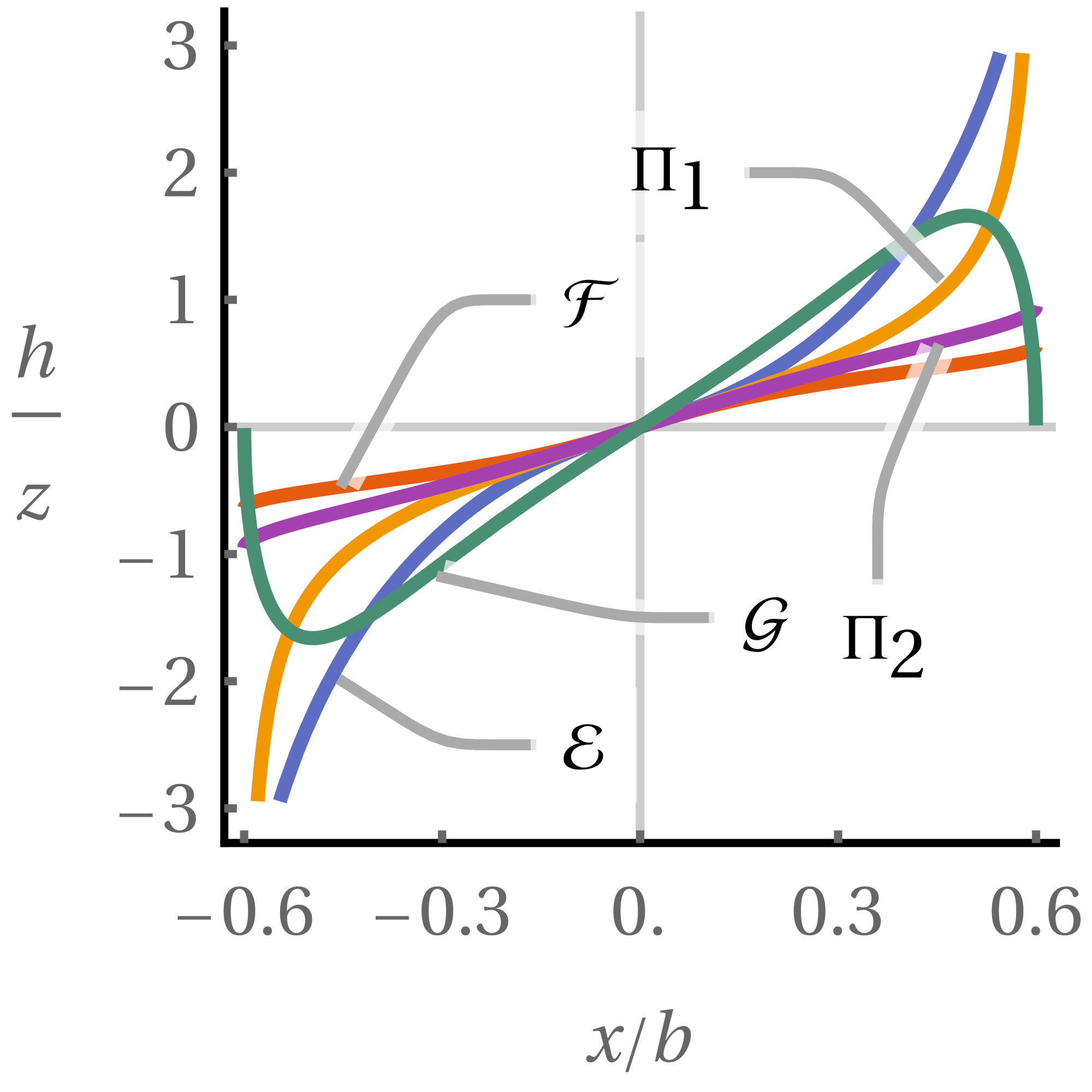
Figure 5: Plots of the 5 basis functions defined in Table (2) for $E=2.245$.

$$\tan\frac{\phi}{2} =n\sin u,\qquad n=\sqrt{\frac{1-a_{2}}{1+a_{2}}},\qquad m=\sqrt{\frac{a_{1}-1}{a_{1}+1}}.$$

By comparison with Table (2) it is easy to see that a linear combination of the 5 functions will span the space of the integrand in Eq.(12). The coefficients $(\alpha\dots\epsilon)$ are given by

$$\begin{aligned} \alpha=&-\frac{c_{0}}{a_{2}}-c_{1}+c_{2}-c_{3},\quad\beta=\frac{(a_{1}-1)(a_{2}+1)c_{0}}{2a_{1}a_{2}},\quad\gamma=c_{0}\left(\frac{1}{a_{1}}+\frac{1}{a_{2}}\right)+2c_{1},\quad\delta=2c_{3},\quad\epsilon=-\frac{(a_{1}-1)(a_{2}-1)c_{0}}{4a_{1}a_{2}}\end{aligned}$$

To find the height $h(x,E)$ we start from the dynamical systems and transform $x$ using Eq.(10) to get

$$h\left(x,E\right) =\int^{\phi}\frac{\frac{E}{2}-v_{0}-\frac{9v_{0}}{8z}\cos\phi^{\prime}-\frac{3v_{0}}{4z}\cos^{3}\phi^{\prime}}{\cos^{2}\phi^{\prime}\sqrt{4v_{A}^{2}-\left(E-\frac{3v_{0}}{4z}\cos\phi^{\prime}\right)^{2}}}\,d\phi^{\prime}$$

$$=\int^{\phi}\frac{\frac{E}{2}-v_{0}-\frac{9v_{0}}{8z}\cos\phi^{\prime}-\frac{3v_{0}}{4z}\cos^{3}\phi^{\prime}}{\cos^{2}\phi^{\prime}\sqrt{\left(2v_{A}-E+\frac{3v_{0}}{4z}\cos\phi^{\prime}\right)\left(2v_{A}+E-\frac{3v_{0}}{4z}\cos\phi^{\prime}\right)}}\,d\phi^{\prime}.$$

The above integral is of the form given in Eq.(11), and thus, can be rendered in the analytic form

$$\frac{4z}{3v_{0}}\left(\alpha\mathcal{F}+\beta\mathcal{E}+\gamma\text{$\Pi$}_{1}+\delta\text{$\Pi$}_{2}+\epsilon\mathcal{G}\right),$$

$$c_{0}=\left(\frac{E}{2}-v_{0}\right),\quad c_{1}=-\frac{9v_{0}}{8z},\quad c_{2}=0,\quad c_{3}=-\frac{3v_{0}}{4z},\quad a_{1}=\frac{4z}{3v_{0}}\left(2v_{A}+E\right),\quad a_{2}=\frac{4z}{3v_{0}}\left(2v_{A}-E\right)$$

The constant of integration can be set to 0 w.l.o.g due to translational invariance in the $z$ direction in the unbounded domain. We can also calculate other useful quantities such as the average sedimentation velocity, the time period of the oscillation and the maximum $h$ amplitude of the closed orbits seen in a co-sedimenting frame of reference

$$\left\langle\dot{h}\right\rangle =\frac{1}{T_{E}}4\int_{0}^{\phi_{\text{m}}}\frac{\dot{\tilde{h}}}{\dot{\phi}}d\phi=4h\left(\phi_{m},E\right)$$

$$T_{E} =4\int_{0}^{\phi_{m}}\frac{d\phi}{\dot{\phi}}=4\int_{0}^{\phi_{\text{m}}}\frac{d\phi}{\sqrt{\left(2v_{A}-E+\frac{3v_{0}}{4z}\cos\phi\right)\left(2v_{A}+E-\frac{3v_{0}}{4z}\cos\phi\right)}\cos^{2}\phi}$$

$$\Delta h =h\left(\phi_{0},E\right)-\int_{0}^{\phi_{\text{0}}}\left\langle\dot{h}\right\rangle\frac{d\phi}{\dot{\phi}}$$

where $\phi_{0}$ is the solution of $\frac{E}{2}-v_{0}-\frac{9v_{0}}{8z}\cos\phi_{0}-\frac{3v_{0}}{4z}\cos^{3}\phi_{0}=0$. In each case the coefficients for the $c_{i}$s can be written down and hence the integral evaluated using Table (2).

	Function	Derivative	Common denominator
$\mathcal{F}$	$\mathcal{F}\left(u,-\frac{n^{2}}{m^{2}}\right)$	$\frac{1}{\sqrt{1+\frac{n^{2}}{m^{2}}\sin^{2}(u)}}$	$\frac{\left(1-n^{2}\sin^{2}u\right)^{2}\left(1+n^{2}\sin^{2}u\right)}{\left(1-n^{2}\sin^{2}u\right)^{2}\left(1+n^{2}\sin^{2}u\right)\sqrt{1+\frac{n^{2}}{m^{2}}\sin^{2}(u)}}$
$\mathcal{E}$	$\mathcal{E}\left(u,-\frac{n^{2}}{m^{2}}\right)$	$\sqrt{1+\frac{n^{2}}{m^{2}}\sin^{2}(u)}$	$\frac{\left(1-n^{2}\sin^{2}u\right)^{2}\left(1+n^{2}\sin^{2}u\right)\left(1+\frac{n^{2}}{m^{2}}\sin^{2}u\right)}{\left(1-n^{2}\sin^{2}u\right)^{2}\left(1+n^{2}\sin^{2}u\right)\sqrt{1+\frac{n^{2}}{m^{2}}\sin^{2}u}}$
$\text{$\Pi$}_{1}$	$\text{$\Pi$}\left(n^{2};u,-\frac{n^{2}}{m^{2}}\right)$	$\frac{1}{\left(1-n^{2}\sin^{2}(u)\right)\sqrt{1+\frac{n^{2}}{m^{2}}\sin^{2}(u)}}$	$\frac{\left(1-n^{2}\sin^{2}u\right)\left(1+n^{2}\sin^{2}u\right)}{\left(1-n^{2}\sin^{2}u\right)^{2}\left(1+n^{2}\sin^{2}u\right)\sqrt{1+\frac{n^{2}}{m^{2}}\sin^{2}u}}$
$\text{$\Pi$}_{2}$	$\text{$\Pi$}\left(-n^{2};u,-\frac{n^{2}}{m^{2}}\right)$	$\frac{1}{\left(1+n^{2}\sin^{2}(u)\right)\sqrt{1+\frac{n^{2}}{m^{2}}\sin^{2}(u)}}$	$\frac{\left(1-n^{2}\sin^{2}u\right)^{2}}{\left(1-n^{2}\sin^{2}u\right)^{2}\left(1+n^{2}\sin^{2}u\right)\sqrt{1+\frac{n^{2}}{m^{2}}\sin^{2}u}}$
$\mathcal{G}$	$\frac{\sin 2u\sqrt{1+\frac{n^{2}}{m^{2}}\sin^{2}u}}{1-n^{2}\sin^{2}u}$	$\frac{2-2\left(2-n^{2}+2\frac{n^{2}}{m^{2}}\right)\sin^{2}u+6\frac{n^{2}}{m^{2}}\sin^{4}u-2n{}^{2}\sin^{6}u}{\left(1-n^{2}\sin^{2}u\right)^{2}\sqrt{1+\frac{n^{2}}{m^{2}}\sin^{2}u}}$	$\frac{\left(1+n^{2}\sin^{2}u\right)\left(2-2\left(2-n^{2}+2\frac{n^{2}}{m^{2}}\right)\sin^{2}u+6\frac{n^{2}}{m^{2}}\sin^{4}u-2n{}^{2}\sin^{6}u\right)}{\left(1-n^{2}\sin^{2}u\right)^{2}\left(1+n^{2}\sin^{2}u\right)\sqrt{1+\frac{n^{2}}{m^{2}}\sin^{2}u}}$

Table 2: The 5 basis functions that make up integral in Eq.(11). $\mathcal{F}$,$\mathcal{E}$,$\Pi$ are incomplete elliptic integrals of the first, second and third kind respectively. These have been plotted in Fig.(5).

III Krylov-Bogolyubov averaging of limit cycle at bottom plane

The constant of the motion

$$H(x,\theta)=\frac{mg}{8\pi\eta}\frac{1}{\sqrt{x^{2}+z^{2}}}+2v_{A}\cos\theta$$

remains a constant if, to first order, perturbations introduced into the equations of motion cancel. Then the perturbations have no effect on the average orbital quantities. Our equations of motion are

$$\dot{\theta} =-\frac{mgx}{8\pi\eta r^{3}}-\omega_{R}\sin\theta$$

$$\dot{x} =\,\,\,\,2v_{A}\sin\theta+\frac{9b^{2}v_{0}^{2}x}{32h^{2}},$$

where the first term on the right hand side is the transient and the second term is the perturbation. The average change of the $H$ over a cycle is given by

$$\left\langle\dot{H}\right\rangle =\int^{T_{E}}\frac{dH}{dt}dt=\int^{T_{E}}\nabla H\cdot\dot{\boldsymbol{x}}dt$$ (13)

$$=\int^{T_{E}}\nabla H\cdot\Delta dt=\oint\frac{\nabla H\cdot\Delta}{\dot{\boldsymbol{x}}}d\boldsymbol{x}$$ (14)

where the transient parts of $\nabla H\cdot\dot{\boldsymbol{x}}$, which are the equations of motion far from the planes, vanish by the symplectic structure. The remaining part needs to be evaluated for the perturbation vector

$$\Delta=\begin{pmatrix}-\omega_{R}\sin\theta\\ \frac{9b^{2}v_{0}^{2}x}{32h^{2}}\end{pmatrix}.$$

We require the period average of $\nabla H\cdot\Delta/\dot{\boldsymbol{x}}$ to vanish to ensure that the average “energy” $E^{*}$ over a cycle remains constant. We define $h^{*}$ to be the period averaged height from the bottom plane. This immediately gives the condition

$$\left\langle\dot{H}\right\rangle =\langle 2\omega_{R}v_{A}\sin^{2}\theta-\frac{9b^{2}v_{0}^{2}x^{2}}{32\left(x^{2}+z^{2}\right)^{3/2}h^{*2}}\rangle$$

$$=\frac{4}{T_{E}}\int_{0}^{x_{m}}\frac{\omega_{R}\left[4v_{A}^{2}-\left(E^{*}-\frac{3bv_{0}}{4\sqrt{x^{2}+z^{2}}}\right)^{2}\right]-\frac{9b^{2}v_{0}^{2}x^{2}}{32\left(x^{2}+z^{2}\right)^{3/2}h^{*2}}}{\sqrt{4v_{A}^{2}-\left(E^{*}-\frac{3bv_{0}}{4\sqrt{x^{2}+z^{2}}}\right)^{2}}}dx$$

$$=0$$

which, under the transformation $x=z\tan\phi$, gives an integral of the form given in Section II. This condition relates the “equilibrium” height $h^{*}$ and “energy” $E^{*}$. A second condition comes from balancing levitation against sedimentation over a cycle immediately giving

$$\left\langle\dot{h}\right\rangle =-\left(v_{0}+E\right)+\langle 3v_{A}\cos\theta-v_{0}\left(\frac{3bz^{2}}{4r^{3}}-\frac{3b}{2h^{*}}\right)\rangle.$$

$$=-\left(v_{0}+E\right)+\frac{4}{T_{E}}\int_{0}^{x_{m}}\frac{\frac{3}{2}\left(E^{*}-\frac{3bv_{0}}{4\sqrt{x^{2}+z^{2}}}\right)-v_{0}\left(\frac{3bz^{2}}{4r^{3}}-\frac{3b}{2h^{*}}\right)}{\sqrt{4v_{A}^{2}-\left(E^{*}-\frac{3bv_{0}}{4\sqrt{x^{2}+z^{2}}}\right)^{2}}}dx$$

$$=0.$$

again this integral can be put in the form of Eq.(11) and thus we arrive at a second condition relating $h^{*}$ and $E^{*}$. These can be solved simultaneously to give a unique estimate for the orbit parameters of the limit cycle near the bottom plane. The pair $\left(E^{*},h^{*}\right)$ is plotted as a function of $\omega_{R}$ in Fig.(3c) in the main text.

IV Exchange of dancing partners

In this section, we consider two pairs of active particles near a plane no-slip and no-shear surface. We emphasize that the qualitative features of bound states predicted in the main text do not depend on the no-slip or no-shear nature of the plane surface. Here, we show that the interaction times at the no-shear surface is much longer compared to a no-slip surface (Thutupalli et al., 2018) and that one of the scattering states involves these interacting pairs exchanging partners.

The monopolar flow around an active colloid near the bottom of a parallel plate geometry is of similar symmetry as that of a contractile dipole (Squires and Brenner, 2000), whose axis is along the normal to the bottom surface. This has the effect of repulsion between the bound states. These contractile flows also produce a torque on the particles in other pairs which rotate nearby neighbours towards one another. Active swimming is then able to bring the two bound pairs towards one another. Repulsion dominates when pairs are separated from each other such that $x\gg z$. On the other hand attraction occurs if $x\sim z$. After the interaction particles can either leave as bound pairs or single particles. Free particles are able to swim up towards the top surface while bound pairs stabilize near the bottom of the cell and continue their dance indefinitely. If a no-slip surface is used instead, the individual dancing behaviour remains the same however the inter-pair interaction is weakened by the no-slip condition. The result is that the timescale for pairs to come into contact is dramatically increased. Otherwise the actual interaction and final states appear qualitatively unchanged (see Fig.(6). We postpone further discussion of this effect to future work. Multiparticle simulations were done with $\omega_{R}=0.02,\,v_{0}=0.3,\,v_{A}=0.3$. The sedimentation force was reduced in these simulations for integrator stability since the effective hydrodynamic forces on particles becomes extremely large when multiple particles come into close proximity.

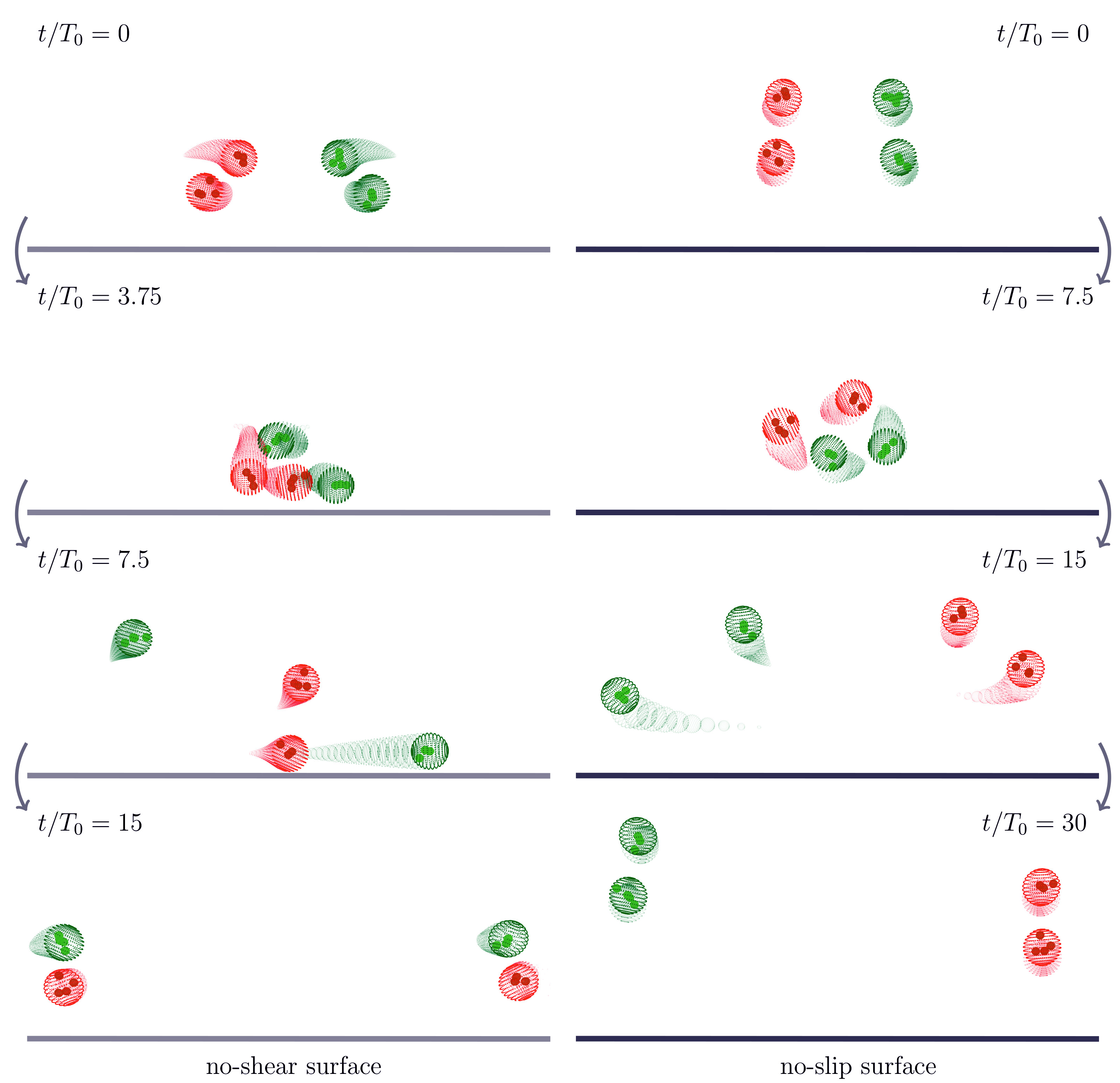
Figure 6: Stroboscopic images of two active bound pairs near a plane no-shear and no-slip surface. The presence of the no-slip condition at the surface weakens hydrodynamic interactions and hence increases the interaction time scale. The particles are pulled down towards the lower surface under the effect of their mutual sedimentation force. Here scattering leads to an exchange of partners in the no-shear geometry and an exchange of places in the no-slip geometry. The end product of scattering events is highly dependent on the initial conditions. See movie 2.

References

- Lighthill (1952) M. J. Lighthill, “On the squirming motion of nearly spherical deformable bodies through liquids at very small Reynolds numbers,” Commun. Pure. Appl. Math. 5, 109–118 (1952).
- Blake (1971a) J. R. Blake, “A spherical envelope approach to ciliary propulsion,” J. Fluid Mech. 46, 199–208 (1971a).
- Anderson (1989) J. L. Anderson, “Colloid transport by interfacial forces,” Annu. Rev. Fluid Mech. 21, 61–99 (1989).
- Lauga and Powers (2009) E. Lauga and T. R. Powers, “The hydrodynamics of swimming microorganisms,” Rep. Prog. Phys. 72, 096601 (2009).
- Drescher et al. (2010) K. Drescher, R. E. Goldstein, N. Michel, M. Polin, and I. Tuval, “Direct measurement of the flow field around swimming microorganisms,” Phys. Rev. Lett. 105, 168101 (2010).
- Koch and Subramanian (2011) D. L. Koch and G. Subramanian, “Collective hydrodynamics of swimming microorganisms: Living fluids,” Annu. Rev. Fluid Mech. 43, 637–659 (2011).
- Marchetti et al. (2013) M. C. Marchetti, J. F. Joanny, S. Ramaswamy, T. B. Liverpool, J. Prost, Madan Rao, and R. A. Simha, “Hydrodynamics of soft active matter,” Rev. Mod. Phys. 85, 1143–1189 (2013).
- Ramaswamy (2017) S. Ramaswamy, “Active matter,” J. Stat. Mech. 2017, 054002 (2017).
- Ghose and Adhikari (2014) S. Ghose and R. Adhikari, “Irreducible Representations of Oscillatory and Swirling Flows in Active Soft Matter,” Phys. Rev. Lett. 112, 118102 (2014).
- Pedley et al. (2016) T. J. Pedley, D. R. Brumley, and R. E. Goldstein, “Squirmers with swirl: a model for Volvox swimming,” Journal of Fluid Mechanics 798, 165–186 (2016).
- Drescher et al. (2009) K. Drescher, K. C. Leptos, I. Tuval, T. Ishikawa, T. J. Pedley, and R. E. Goldstein, “Dancing Volvox: Hydrodynamic bound states of swimming algae,” Phys. Rev. Lett. 102, 168101 (2009).
- Goldstein (2015) R. E. Goldstein, “Green algae as model organisms for biological fluid dynamics,” Ann. Rev. Fluid Mech. 47, 343–375 (2015).
- Palacci et al. (2013) J. Palacci, S. Sacanna, A. P. Steinberg, D. J. Pine, and P. M. Chaikin, “Living crystals of light-activated colloidal surfers,” Science 339, 936–940 (2013).
- Palacci et al. (2010) J. Palacci, C. Cottin-Bizonne, C. Ybert, and L. Bocquet, “Sedimentation and Effective Temperature of Active Colloidal Suspensions,” Phys. Rev. Lett. 105, 088304 (2010).
- Buttinoni et al. (2013) I. Buttinoni, J. Bialké, F. Kümmel, H. Löwen, C. Bechinger, and T. Speck, “Dynamical Clustering and Phase Separation in Suspensions of Self-Propelled Colloidal Particles,” Phys. Rev. Lett. 110, 238301 (2013).
- Ebbens and Howse (2010) S. J. Ebbens and J. R. Howse, “In pursuit of propulsion at the nanoscale,” Soft Matter 6, 726–738 (2010).
- Smoluchowski (1911) M. Smoluchowski, “On the mutual action of spheres which move in a viscous liquid,” Bull. Acad. Sci. Cracovie A 1, 28–39 (1911).
- Brenner (1963) H. Brenner, “The Stokes resistance of an arbitrary particle,” Chem. Engg. Sci. 18, 1–25 (1963).
- Ladd (1988) A. J. C. Ladd, “New1 Hydrodynamic interactions in a suspension of spherical particles,” J. Chem. Phys. 88, 5051–5063 (1988).
- Squires and Brenner (2000) T. M. Squires and M. P. Brenner, “Like-Charge Attraction and Hydrodynamic Interaction,” Phys. Rev. Lett. 85, 4976–4979 (2000).
- Squires (2001) T. M. Squires, “Effective pseudo-potentials of hydrodynamic origin,” J. Fluid Mech. 443, 403–412 (2001).
- Singh and Adhikari (2016) R. Singh and R. Adhikari, “Universal hydrodynamic mechanisms for crystallization in active colloidal suspensions,” Phys. Rev. Lett. 117, 228002 (2016).
- Nash et al. (2010) R. W. Nash, R. Adhikari, J. Tailleur, and M. E. Cates, “Run-and-Tumble Particles with Hydrodynamics: Sedimentation, Trapping, and Upstream Swimming,” Phys. Rev. Lett. 104, 258101 (2010).
- Singh et al. (2015) R. Singh, S. Ghose, and R. Adhikari, “Many-body microhydrodynamics of colloidal particles with active boundary layers,” J. Stat. Mech 2015, P06017 (2015).
- (25) In this limit, the Green’s function can be approximated by that of an unbounded or semi-unbounded geometry.
- Singh and Adhikari (2018) R. Singh and R. Adhikari, “Generalized Stokes laws for active colloids and their applications,” J. Phys. Commun. 2, 025025 (2018).
- (27) “See Supplemental Material at [to be inserted] which includes the details of the calculations, simulation details, and movies of dynamics.” .
- Pozrikidis (1992) C. Pozrikidis, Boundary Integral and Singularity Methods for Linearized Viscous Flow (Cambridge University Press, 1992).
- Pedley and Kessler (1992) T. J. Pedley and J. O. Kessler, “Hydrodynamic phenomena in suspensions of swimming microorganisms,” Annu. Rev. Fluid Mech. 24, 313–358 (1992).
- (30) Gravitational torque therefore also provides robustness to the dynamics against out-of-plane perturbations.
- (31) Any divergence-free vector field in 2-dimensions is a Hamiltonian flow (Arnold, 2013).
- Arnold (2013) V. I. Arnold, Mathematical methods of classical mechanics, Vol. 60 (Springer, New York, 2013).
- Gradshteyn and Ryzhik (2014) I.S. Gradshteyn and I.M. Ryzhik, “Table of Integrals, Series, and Products,” (Academic Press, 2014) pp. 63–247.
- Krylov and Bogoli︠u︡bov (1947) N.M. Krylov and N. N. Bogoli︠u︡bov, Introduction to non-linear mechanics (Princeton Univ. Press, 1947).
- (35) The reason for this discrepancy is that (Drescher et al., 2009) do not consider the height to be dynamical and fix it, by fiat, to a constant value, around which linear stability is examined.
- (36) A. Bolitho . , “Flow-induced bound states of active particles,” In preparation .
- Fodor et al. (2016) É. Fodor, C. Nardini, M. E. Cates, J. Tailleur, P. Visco, and F. van Wijland, “How Far from Equilibrium Is Active Matter?” Phys. Rev. Lett. 117, 038103 (2016).
- R. Singh and Adhikari (2019) R. Singh and R. Adhikari, “Hydrodynamic and phoretic interactions of active particles in Python,” arXiv:1910.00909 (2019).
- Blake (1971b) J. R. Blake, “A note on the image system for a Stokeslet in a no-slip boundary,” Proc. Camb. Phil. Soc. 70, 303–310 (1971b).
- Aderogba and Blake (1978) K. Aderogba and J. R. Blake, “Action of a force near the planar surface between semi-infinite immiscible liquids at very low Reynolds numbers,” Bull. Australian Math. Soc. 19, 309–318 (1978).
- Ishikawa et al. (2020) T. Ishikawa, T. J. Pedley, K. Drescher, and Raymond E. Goldstein, “Stability of dancing Volvox,” (2020), arXiv:2001.02825 [physics.flu-dyn] .
- Thutupalli et al. (2018) S. Thutupalli, D. Geyer, R. Singh, R. Adhikari, and H. A. Stone, “Flow-induced phase separation of active particles is controlled by boundary conditions,” Proc. Natl. Acad. Sci. 115, 5403–5408 (2018).