Medium-band photometric reverberation mapping of AGNs at $0.1<z<0.8$

Abstract

The most popular method of the broad-line region size estimation in active galactic nuclei (AGN) is the reverberation mapping based on measuring the time delay between the continuum flux and the flux in the emission lines. In our work, we apply the method of photometric reverberation mapping in mid-band filters, adapted for observations on the 1-m Zeiss-1000 telescope of Special Astrophysical Observatory of Russian Academy of Sciences, for the study of AGN with broad lines in the range of redshifts $0.1<z<0.8$. This paper provides a sample of 8 objects, describes the technique of observations and data processing for 2 studied objects to demonstrate the stability of the used method.

1 Introduction

Active galactic nuclei (AGN) are bright compact areas, emitting up to 90% of the energy of the entire galaxy. Because of the small size of the central object and the high gas velocity, it is now assumed that the supermassive black hole (SMBH) is present in the center of the galactic nucleus, and the enormous luminosity is provided by the processes of the matter accretion into the SMBH. The observed energy distribution, as well as the AGN spectrum, indicates that the nucleus is a multicomponent system, which observational properties depend on the orientation relative to the observer. This is known as the Unified model (Antonucci, 1993; Urry & Padovani, 1995), which is illustrated in Fig. 1. According to this model, the SMBH is surrounded by a hot disk of accreting matter ($\sim$0.001 pc from the central source), which hard radiation excites the gas in the broad-line region (BLR) at scales of 0.01-0.1 pc and is re-emitted in emission lines broadened due to the high gas velocity (up to $10^{4}$ km/s).

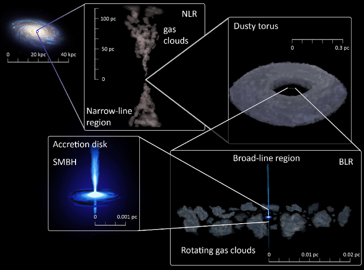
Figure 1: The illustration of modern conceptions of AGN structure.

The reverberation mapping method (RM, Blandford & McKee, 1982) consists of measuring the time lag $\tau$ between the continuum radiation of the accretion disk and the radiation in the emission lines produced in the BLR in AGN. The BLR size is assumed to be $R_{\rm BLR}\equiv c\tau$, where $c$ is the speed of light (Peterson, 1993). Then, the $R_{\rm BLR}$ can be determined by measuring the time lag $\tau$ between the continuum and line light curves. According to the virial ratio the SMBH mass is related to the BLR size $c\tau$ and the gas velocity in the BLR $\upsilon_{\rm line}$ as:

$$M_{\rm SMBH}=fc\tau\upsilon_{\rm line}^{2}G^{-1},$$

where $G$ is the gravitational constant and $f$ is a dimensionless factor of the order of one depending on the BLR structure and kinematics and the inclination of the system relative to the observer. Thus, measuring the time delays provides one with the SMBH mass estimation. Yet, the RM method requires the accumulation of a long series of observational data that makes harder its wide application. That is the reason why presently this method was applied only for approximately 100 nearest quasars (e.g. Shapovalova et al., 2009; Bentz & Katz, 2015; Du et al., 2016; Jiang et al., 2016; Pozo Nuñez et al., 2017; Ilić et al., 2017).

However, to trace the evolution of the SMBH masses the extension of the AGN sample with known sizes $R_{\rm BLR}$ to more distant redshifts is needed. For AGN the linear relation between the BLR size and AGN luminosity was found: $R_{\rm BLR}\propto L^{\alpha}$, where $L$ could be measured in different spectral bands such as 5100Å (Kaspi et al., 2005; Bentz et al., 2009b) or definite emission lines (e.g. MgII in Czerny et al., 2019, and references therein).

Our investigation is dedicated to complement the existing relation of $R_{\rm BLR}(L)$ by new measurements of $R_{\rm BLR}$ = $c\tau$ for the distant AGNs up to $z\sim 0.8$ using a sample of objects that have not been studied in other reverberation campaigns. Besides, we adopt the photometric RM method (Haas et al., 2011) to mid-band observation with the 1-meter class telescope.

The paper is formed as following. In Sec. 2 the sample and the methods of observations and data reduction are given. Sec. 3 contains the first results of the applied observational technique with the description of the local standards and the preliminary light curves. The conclusions and main ideas are shortly given in Sec. 4.

2 Observations

2.1 Sample

Our sample consists of 8 AGNs with broad lines (equivalent width $W_{\lambda}>200$Å) in the range the redshifts $0.1<z<0.8$ with the brightness limited to $m<$ 20 mag. The sample includes only near-polar objects (Dec $>68^{\circ}$), thus we were able to observe them throughout the whole year. The final sample is shown in Table 1.

	Name	RA Dec	Mag	$z$	$\tau$	Filters
(#)	(1)	(2)	(3)	(4)	(5)	(6)
1	2MASX J08535955+7700543	08h53m59s.4 $+77^{\circ}00^{\prime}55^{\prime\prime}$	$17.0$	0.106	$27$	SED725 SED700
2	VII Zw 244	08h44m45s.3 $+76^{\circ}53^{\prime}09^{\prime\prime}$	$15.7$	0.131	$34$	SED550 SED525
3	SDSS J093702.85+682408.3	09h37m02s.9 $+68^{\circ}24^{\prime}08^{\prime\prime}$	$18.0$	0.294	$47$	SED625 SED600
4	SDSS J094053.77+681550.3	09h40m53s.8 $+68^{\circ}15^{\prime}50^{\prime\prime}$	$19.4$	0.371	$59$	SED900 SED875
5	SDSS J100057.50+684231.0	10h00m57s.5 $+68^{\circ}42^{\prime}31^{\prime\prime}$	$19.0$	0.499	$80$	SED725 SED700
6	2MASS J01373678+8524106	01h37m36s.7 $+85^{\circ}24^{\prime}11^{\prime\prime}$	$16.6$	0.499	$79$	SED725 SED700
7	SDSS J095814.46+684704.8	09h58m14s.4 $+68^{\circ}47^{\prime}05^{\prime\prime}$	$19.7$	0.662	$92$	SED800 SED775
8	GALEX 2486024515200490156	10h01m51s.6 $+69^{\circ}35^{\prime}27^{\prime\prime}$	$19.6$	0.847	$124$	SED900 SED875

Table 1: Observed sample of AGN: (#) identification number in the sample; (1) galaxy name; (2) coordinates for the J2000 epoch; (3) magnitude in $V$ band; (4) redshift $z$; (5) roughly estimated time delay $\tau$ in days from the continuum or emission line luminosity (see text for details); (6) filters used to measure line and continuum fluxes.

Each object is observed in two filters selected so that they cover the broad emission line H_β(α) and the near-by continuum, which was used to subtract the contribution of the variable continuum from the emission line. The experiment uses medium-band interference filters with the spectral energy distribution (SED) of a 250Å bandwidth, covering the 5000–9000Å  range with 250Å-step. The selection of filters with their bandwidth overplotted on the spectra of the studied objects is illustrated in Fig. 2. The spectra are taken from Abolfathi et al. (2018), Boroson & Green (1992), and Wei et al. (1999).

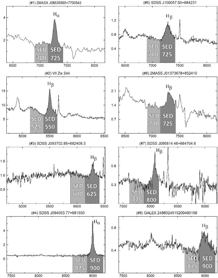
Figure 2: SED filters bands overplotted on the spectra of the studied AGN. Flux $F_{\lambda}$ in units of $10^{-16}$ erg/cm²/s/Å depending on the wavelength in Å given in the observer rest frame. The spectra of #1 and #6 are obtained from Wei et al. (1999), #2 is from Boroson & Green (1992) and the others are from Abolfathi et al. (2018).

From the known radius-luminosity relation $R_{\rm BLR}-L$ for the H_β line the expected time delays $\tau$ were calculated for the sample (see Table 1, column 5) in the following way. For the objects with redshifts up to 0.5 - objects #1,3-5 - the flux $F_{\lambda}$ at 5100Å was integrated in the range 4400-5850Å in the rest frame from the spectra obtained from the literature; the flux $F_{\lambda}$ was divided by the window-width in order to get the monochromatic luminosity. The 4400-5850Å range contains some strong emission lines as variable H_β and approximately constant O[III] but as the integrated band is wide we assume that the lines contribution is not crucial especially for rough estimation of the time delays. To convert the flux to the luminosity $L_{\lambda}$ at 5100 Å  it was multiplied with $4\pi D^{2}$, where $D$ is the AGN luminosity distance calculated using the cosmological parameters $\Omega_{0}=0.3036$ and $H_{0}=68.14$ km/s/Mpc. Note here that the contribution of the host galaxy was not considered. Then we applied the relation $R_{\rm BLR}-L_{\lambda}({5100})$:

$$\lg(R_{\rm BLR})=-21.3^{+2.9}_{-2.8}+0.519^{+0.063}_{-0.066}\lg(\lambda L_{\lambda}),$$

where $L_{\lambda}=L_{\lambda}({5100})$ is a luminosity at 5100Å, and $R_{\rm BLR}$ is the BLR size in the H_β line (Bentz et al., 2009a).

In the case of $z>0.5$, as well as for the object #2, which spectral data used by us in calculations are available only in a small wavelength range (4075-5883Å), the $L_{\lambda}({5100})$ range goes beyond the available optical spectra. In this regard, for objects #2,6-8 we used the relation with the line $L_{\lambda}({\rm H}_{\beta})$ from Greene et al. (2010):

$$\lg(R_{10})=0.85\pm 0.05+(0.53\pm 0.04)\lg[L_{43}({\rm H}_{\beta})],$$

where $R_{10}=R_{\rm BLR}/10$ lt days is the size of the BLR region, normalized to 10 lt days, $L_{43}({\rm H}_{\beta})=L_{\lambda}({\rm H}_{\beta})/10^{43}$ erg/s is the luminosity in the H_β line, normalized to $10^{43}$ erg/s. In Table 1 the rough estimate of the expected time delays $\tau$ are given with an accuracy of 10%.

2.2 Observational technique and reduction

Since February 2018, observations of the AGN sample have been carried out monthly on gray and bright nights at 1-m Zeiss-1000 telescope of the Special Astrophysical Observatory of Russian Academy of Sciences (SAO RAS) using MaNGaL (MApper of Narrow GAlaxy Lines, Perepelitsyn et al., 2018) and MMPP (Multi-Mode Photometer-Polarimeter) devices in photometric mode with 10 medium-band interference SED filters. The size of the field of view (FoV) was 8.${}^{\prime}7\times 8.^{\prime}7$ for MaNGaL and 7.${}^{\prime}2\times 7.^{\prime}$2 for MMPP. Up to now, around 15 epochs were acquired on average for majority of the objects in the sample.

Three different detectors were used during the observations: Andor CCD iKon-M 934 (1024$\times$1024 px), Andor Neo sCMOS (2560$\times$2160 px) and Raptor Photonics Eagle V CCD (2048$\times$2048 px). The quantum efficiency of these receivers in the needed bands is shown in Table 2. Water cooling was used for all three cases to minimize noise.

Detector	5500Å	6000Å	7000Å	8000Å	9000Å
Andor iKon-M 934	95%	96%	91%	77%	47%
Andor Neo sCMOS	54%	56%	49%	31%	14%
Raptor Eagle V CCD	92%	95%	89%	75%	50%

Table 2: Quantum efficiency of detectors in the studied photometric bands.

Observations of the sample were alternated with observations of spectrophotometric standard stars provided by Oke (1990). The standards were observed almost simultaneously with the object field in the same filter to minimize the variations of atmospheric transmission; moreover, even observing the standards at the close zenith distance we tried to obtain the extinction coefficient every night and take it into account. Such strategy was used to create a list of comparison stars with known AB-magnitudes in the FoV of the sample.

During each observational night, we received calibration images (flat frames at the twilight sky for each filter, bias/dark) to correct data for additive and multiplicative errors. For each object the series of images (3 and more) were taken, the exposure times depend on the object brightness, weather conditions and are ranged from 2 to 10 minutes. For correct statistics each frame is processed independently, and statistical evaluation is made by averaging the random value by robust methods giving its unbiased estimate. In this case, the photometric errors are the rms of the robust distribution.

The method of aperture photometry was used to determine the absolute flux of the objects in instrumental units. Therefore, to correctly estimate the sky background, the traces of cosmic rays which were close to the object were removed from images.

For better photometric accuracy needed for the variability studies of AGN, the AB fluxes were first calculated using the spectrophotometric standards, and further step was to re-calibrate them with the differential photometry using the local standards from the object image FoV.

3 Results

3.1 Local standards

The main methodological result obtained during the first year of observations is the definition of local standards in the field of each sample objects. In Fig. 3 we show the field of the object #1 (2MASX J08535955+7700543) obtained in the SED725 filter and object #2 (VII Zw 244) obtained in the SED550 filter by Raptor Eagle V CCD (MMPP) with marked local standards. Within the stable photometric nights, we bind the field with known spectrophotometric standards. To examine the variability of the stars in the fields, the obtained fluxes were normalized to the most frequently observed and the most stable star flux. Thus, the resulting fluxes of stars do not depend on weather conditions on the selected night. Fig. 4 presents the normalized light curves of local standards in objects #1 and #2 fields in AB-magnitudes. In Fig. 4 the regions corresponding to the 3$\sigma$ confidence area are also shown. For differential photometry, the stars with the smallest scatter were chosen. It is also seen that the average error of the absolute binding was of the order of 0.03 mag.

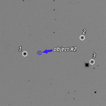
Figure 3: Direct images of AGNs: the object #1 obtained in the SED725 filter with 6 local standards candidates marked (left) and object #2 obtained in the SED550 filter by CCD Eagle V [MMPP] with 3 local standards candidates marked (right).

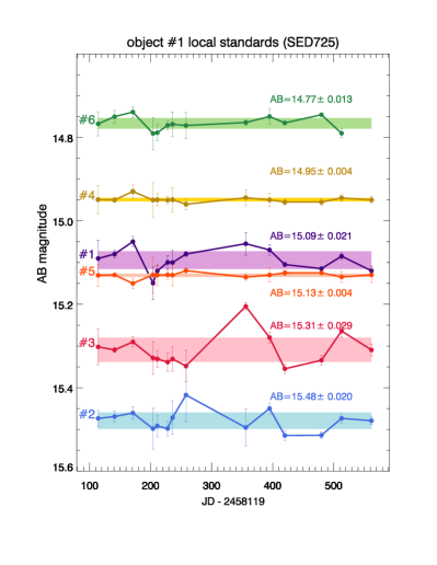
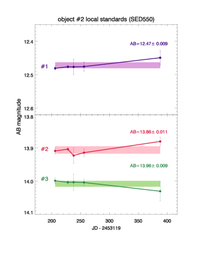
Figure 4: The light curves of the local standards candidates: 6 stars for object #1 in SED725 (left) and 3 stars for object #2 in SED550 filter (right).

Once local standards have been defined, the flux of the object is measured relatively to them, minimizing errors introduced by variations in the atmosphere.

3.2 First light of light curves

The fluxes of the studied AGN were carried out relatively to the most stable reference stars — local standards. The light curves in the continuum and the line for one of the most intensively observed AGN, object #1 are presented in Fig. 5, left. Also, in Fig. 5, right, the same light curves for object #2 are shown.

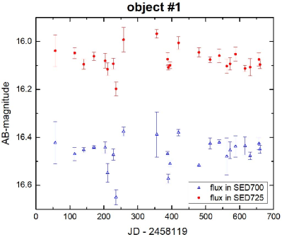
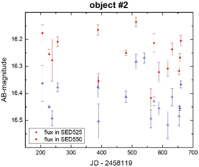
Figure 5: The light curves of object #1 (left) and object #2 (right) in the line (circles) and near-by continuum (triangles). The Julian dates starts on January 1, 2018.

To investigate the time lag between the light curves we have used the JAVELIN code (Zu et al., 2016; Mudd et al., 2018). The first step is to build a continuum model to determine the dumped random walk (DRW) parameters of the continuum light curve. As a result, the posterior distribution of the two DRW parameters (amplitude and timescale) of the continuum variability is calculated by JAVELIN using Markov chain Monte Carlo (MCMC). The second step is to interpolate the continuum light curve based on the posteriors derived on the first step, and then to shift, smooth, and scale each continuum light curve to compare with the observed line light curve. Finally, it derives the posterior distribution of the time lag and other parameters.

Fig. 6 shows the posterior distribution of JAVELIN time delays for objects #1 and #2. This is a distribution of the number of hits N during the MCMC sampling, which sum across all bins gives the sample size. We used at least 10,000 samples. Solid red line marks position of the local peak median, whereas dashed blue line marks expected lag from calibration relations (Table 1, column 5). Our preliminary lags are 44.9${}^{+13.8}_{-12.7}$  and 30.9${}^{+15.1}_{-12.2}$  days for objects #1 and #2 respectively. Low and high estimates of the lags correspond to the highest posterior density interval calculated by JAVELIN.

3.2.1 JAVELIN analysis for object #1

The JAVELIN method involves sampling using the DRW, which ultimately gives us slightly different results from one chain to another. In general, the overall picture for the data set can be traced, however, we can choose the clearest histograms for analysis.
In case of the object #1, we see a stable result for 24 epochs (Fig. 6, left panel):

1. the most powerful peak with a median value of $\sim$45 days is near the expected time delay from the calibrations;

2. the second and the less significant peak appears with a median value of $\sim$125 days.
   

The expected value from the calibration relation for the object #1 is $\sim$27 days, and we confidently take the position of a powerful peak $\tau_{1}=$ 44.9${}^{+13.8}_{-12.7}$  days as a preliminary result.
Clearly, with an increase in the number of epochs, we can reveal a narrowing of the main peak, thereby reducing the error in estimating the time delay value.

3.2.2 JAVELIN analysis for object #2

For the object #2, the number of epochs is only 17, and we see a less clear picture (Fig. 6, right panel). For the range of time delays from 0 to 150 days sampling results are divided into two main solutions with a comparable level of significance:

• peak at $\sim$30 days, which is quite close to the value expected from the calibrations;

• wider peak with a median value of $\sim$90 days.

Despite the fact that we see two comparable peaks, we prefer the first peak, which is closer to the expected value $\sim$34 days from calibrations. An additional argument is that with an increase in the number of epochs we trace the growth of the first peak and hope to see this trend after additional observations. So, for the object #2 we take $\tau=$ 30.9${}^{+15.1}_{-12.2}$  days as a rough preliminary result.
The peaks are wide and still indistinguishable, so more data are needed for a more clear histogram.

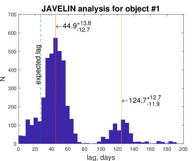
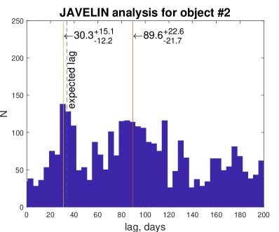
Figure 6: The time lag posterior distributions using JAVELIN code for the object #1 (left) and objects #2 (right). Solid red lines indicate significant peaks and their values, and the expected values from calibrations are indicated by dashed blue lines.

3.2.3 General comments

We should not exclude the possibility of mismatch between the roughly expected time delays and the obtained peaks in the histogram, since the observed luminosity of AGN is variable. That is, the fainter the state of the nucleus we observe, the smaller BLR size estimate is. Moreover, the spectral data for objects #1 and #2 were obtained more than 20 years ago, so the new spectral observation should be done. Also, certainly, the effect of sparse and poor sampling and low number of epochs influence the analysis of light curves. Obviously, we would increase the number of epochs and to clarify our results further we would also compare different cross-correlation methods.

4 Conclusions

In this paper we present the first results of the photometric reverberation mapping project started in 2018 on the 1-m telescope of SAO RAS. The ongoing project is focused on the regular observations of the sample of 8 broad line AGNs, and here the technique of observation and data reduction is shown and the preliminary results demonstrating the method stability. Within this work, the following was obtained.

1. The observations by the photometric reverberation mapping method are adapted for telescopes of 1-meter class and are independent of the device used.

2. For each of the studied AGN in the range of redshifts $0.1<z<0.8$, a list of local standards was determined, which allows further use of the differential photometry method. The photometric accuracy is on average 0.03 mag, which is an order of magnitude greater than the expected amplitude of the AGN variability.

3. The use of the JAVELIN analysis revealed time delays $\tau_{1}=$ 44.9${}^{+13.8}_{-12.7}$  and $\tau_{2}=$ 30.9${}^{+15.1}_{-12.2}$  days for objects #1 and #2, respectively.

It is clear that the first obtained results are in agreement, within the error-bars, with our predictions based on the empirical radius-luminosity relations. However, the data should be processed more carefully and other cross-correlation methods should be applied to reveal whether the calculated time delays are correct. Also, it is particularly important to clean the series from the additional harmonics. Presently, for the majority of the objects the sampling of the observations and the number of epochs is still not sufficient for the reliable analysis, and this is probably the reason why the cross-correlation peaks are so wide. We continue with the observations and in the next stage of the project we are going to obtain and analyze more data, and compare different cross-correlation methods.

References

- Abolfathi et al. (2018) Abolfathi B., et al., 2018, ApJS, 235, 42
- Antonucci (1993) Antonucci R., 1993, ARA&A, 31, 473
- Bentz & Katz (2015) Bentz M. C., Katz S., 2015, PASP, 127, 67
- Bentz et al. (2009a) Bentz M. C., Peterson B. M., Netzer H., Pogge R. W., Vestergaard M., 2009a, ApJ, 697, 160
- Bentz et al. (2009b) Bentz M. C., et al., 2009b, ApJ, 705, 199
- Blandford & McKee (1982) Blandford R. D., McKee C. F., 1982, ApJ, 255, 419
- Boroson & Green (1992) Boroson T. A., Green R. F., 1992, ApJS, 80, 109
- Czerny et al. (2019) Czerny B., et al., 2019, arXiv e-prints, p. arXiv:1901.09757
- Du et al. (2016) Du P., et al., 2016, ApJ, 825, 126
- Greene et al. (2010) Greene J. E., et al., 2010, ApJ, 723, 409
- Haas et al. (2011) Haas M., Chini R., Ramolla M., Pozo Nuñez F., Westhues C., Watermann R., Hoffmeister V., Murphy M., 2011, A&A, 535, A73
- Ilić et al. (2017) Ilić D., et al., 2017, Frontiers in Astronomy and Space Sciences, 4, 12
- Jiang et al. (2016) Jiang L., Shen Y., McGreer I. D., Fan X., Morganson E., Windhorst R. A., 2016, ApJ, 818, 137
- Kaspi et al. (2005) Kaspi S., Maoz D., Netzer H., Peterson B. M., Vestergaard M., Jannuzi B. T., 2005, ApJ, 629, 61
- Mudd et al. (2018) Mudd D., et al., 2018, ApJ, 862, 123
- Oke (1990) Oke J. B., 1990, AJ, 99, 1621
- Perepelitsyn et al. (2018) Perepelitsyn A. E., Moiseev A. V., Oparin D. V., 2018, in Proceedings of the VII Pulkovo astronomical conference for young astronomers (Pulkovo, St. Petersburg, 28 – 31 may 2018). pp 65–70
- Peterson (1993) Peterson B. M., 1993, PASP, 105, 247
- Pozo Nuñez et al. (2017) Pozo Nuñez F., Chelouche D., Kaspi S., Niv S., 2017, PASP, 129, 094101
- Shapovalova et al. (2009) Shapovalova A. I., et al., 2009, New Astronomy Reviews,, 53, 191
- Urry & Padovani (1995) Urry C. M., Padovani P., 1995, PASP, 107, 803
- Wei et al. (1999) Wei J. Y., Xu D. W., Dong X. Y., Hu J. Y., 1999, A&AS, 139, 575
- Zu et al. (2016) Zu Y., Kochanek C. S., Kozłowski S., Peterson B. M., 2016, ApJ, 819, 122