One Man’s Trash is Another Man’s Treasure:
Resisting Adversarial Examples by Adversarial Examples

Abstract

Modern image classification systems are often built on deep neural networks, which suffer from adversarial examples—images with deliberately crafted, imperceptible noise to mislead the network’s classification. To defend against adversarial examples, a plausible idea is to obfuscate the network’s gradient with respect to the input image. This general idea has inspired a long line of defense methods. Yet, almost all of them have proven vulnerable.

We revisit this seemingly flawed idea from a radically different perspective. We embrace the omnipresence of adversarial examples and the numerical procedure of crafting them, and turn this harmful attacking process into a useful defense mechanism. Our defense method is conceptually simple: before feeding an input image for classification, transform it by finding an adversarial example on a pretrained external model. We evaluate our method against a wide range of possible attacks. On both CIFAR-10 and Tiny ImageNet datasets, our method is significantly more robust than state-of-the-art methods. Particularly, in comparison to adversarial training, our method offers lower training cost as well as stronger robustness.

1 Introduction

Deep neural networks have vastly improved the performance of image classification systems. Yet they are prone to adversarial examples. Those are natural images with deliberately crafted, imperceptible noise, aiming to mislead the network’s decision entirely [5, 41]. In numerous applications, from face recognition authorization to autonomous cars [36, 43], the vulnerability caused by adversarial examples gives rise to serious security concerns and presses for efficient defense mechanisms.

The defense, unfortunately, remains grim. Recent studies [34, 45, 12] suggest that the prevalence of adversarial examples may be an inherent property of high-dimensional natural data distributions. Facing this intrinsic difficulty of eliminating adversarial examples, a plausible thought is to conceal them—making them hard to find. Indeed, a long line of works aims to obfuscate the network model’s gradient with respect to its input [50, 14, 49, 7, 39, 33], motivated by the fact that the gradient information is essential for crafting adversarial examples: the gradient indicates how to perturb the input to alter the network’s decision.

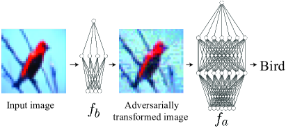
Figure 1: A simple and effective defense mechanism. Given an input image, our defense method first transforms it through the process of crafting adversarial examples on a pre-trained simple model $f_{b}$, deliberately adding strong adversarial noise. The transformed image is then fed into another model $f_{a}$ for classification. The same pipeline is applied in both training and inference.

Yet, almost all these gradient obfuscation based defenses have proven vulnerable. In their recent seminal work, Athalye et al. [2] presented a suite of strategies for estimating network gradients in the presence of gradient obfuscation. Adversarial examples crafted by their method have successfully fooled many existing defense models, some of which even yield 0% accuracy under their attack.

We revisit the idea of gradient obfuscation but take a radically different approach. Instead of expelling adversarial examples, we embrace them. Instead of obstructing the way of finding adversarial examples on a model, we exploit it to strengthen the robustness of another model.

Our defense is conceptually simple: before feeding an input image to a classification model, we transform it through the process of finding adversarial examples on an external model. Mathematically, if we use $f(\bm{x})$ to denote the model that classifies an input image $\bm{x}$, our defense model is expressed as $f(g(\bm{x}))$, where $g(\cdot)$ represents the process of finding an adversarial example near $\bm{x}$ on a pre-trained external model (see Fig. 1).

The robustness of our defense model $f(g(\bm{x}))$ stems from the fundamental difficulties of estimating the gradient of $g(\bm{x})$ with respect to $\bm{x}$. Finding an adversarial example amounts to searching for a local minimum on a highly fluctuated objective landscape [26]. As a result, $g(\bm{x})$ is not an analytic function, not smooth, not deterministic, but an iterative procedure with random initialization and non-differentiable operators. We show that all these traits together constitute a highly robust defense mechanism.

We play devil’s advocate in attacking our defense model thoroughly. We examine a wide range of possible attacks, including those having successfully circumvented many previous defenses [2]. Under these attacks, we compare the worst-case robustness of our method with state-of-the-art defense methods on both CIFAR-10 and Tiny ImageNet datasets. Our defense demonstrates superior robustness over those methods. Particularly, in comparison to models optimized with adversarial training—by far the most effective defense against white-box attacks—our method offers simultaneously lower training cost and stronger robustness.

2 Related Work

Adversarial attack.

The seminal work of Biggio et al. [5] and Szegedy et al. [41] first suggested the existence of adversarial examples that can mislead deep neural networks. The latter also used a constrained L-BFGS to find adversarial examples. Goodfellow et al. [13] later introduced Fast Gradient Sign Method (FGSM) that generates adversarial examples more efficiently. Madry et al. [26] further formalized the problem of adversarial attacks and proposed Projected Gradient Descent (PGD) method, which further inspires many subsequent attacking methods [11, 8, 28, 19]. PGD-type methods are considered the strongest attacks based on first-order information, namely the network’s gradient with respect to the input [26]. To compute the gradients, the adversary must have full access to the network structure and parameters. This scenario is referred as the white-box attack.

When the adversary has no knowledge about the model, the attack, referred as black-box attack, is not as easy as the white-box attack. By far the most popular black-box attack is the so-called transfer attack, which uses adversarial examples generated on a known model (e.g., using PGD) to attack an unknown model [30]. Several methods (e.g., [44, 3, 52, 16]) are proposed to improve the transferability of the adversarial examples so that the adversarial examples generated on one model are more likely to fool another model. Another type of black-box attacking methods is query-based [6, 37, 9, 1, 20]: they execute the model many times with different input in order to learn the behavior of the model and construct adversarial examples.

While our defense is motivated by attacks in white-box scenarios, we evaluate our method under a wide range of possibilities, including both white-box and black-box attacks.

Adversarial defense.

The threat of adversarial examples has motivated active studies of defense mechanisms. By far the most successful defense against white-box attacks is adversarial training [26, 13, 38], and a rich set of methods has been proposed to accelerate its training speed or further improve its robustness [51, 54, 21, 13, 46, 35, 53, 29, 27]. In comparison to adversarial training, our method offers both stronger robustness and lower training cost.

To defend against gradient-based attacks (such as the PGD attack), a natural idea is to obfuscate (or mask) network gradients [30, 44]. To this end, there exist a long line of works that apply random transformation to input images [50, 14], or employ stochastic activation functions [10] and non-differentiable operators in the model [49, 7, 39, 33].

Unfortunately, many of these methods have proven vulnerable by Athalye et al. [2], who introduced a set of attacking strategies, including a method called Backward Pass Differentiable Approximation (BPDA), to circumvent gradient obfuscation (see further discussion in Sec. 3.1 and 3.3). Since then, a few other gradient obfuscation based defenses have been proposed [23, 31, 17, 42, 22]. But those works either report degraded robustness under BPDA attacks [23, 31] or neglected the evaluation against BPDA attacks [17, 42, 22].

Thus far, gradient obfuscation is generally considered vulnerable (and at least incomplete) [2]. We revisit gradient obfuscation, and our defense demonstrates unprecedented robustness against BPDA and other possible attacks.

3 Defense via Adversarial Transformation

We now present a simple approach to defend against adversarial attacks. We will first motivate and describe our adversarial transformation (Sec. 3.1 and 3.2), and then provide the rationale of why it improves adversarial robustness (Sec. 3.3 and 3.4), backed by empirical evidence (Sec. 4).

3.1 Motivation: Input Transformation

An attempt that has been explored in adversarial defense—albeit unsuccessfully so far—is the defense via input transformation. Consider a neural network model $f_{a}$ that classifies the input image $\bm{x}$ (i.e., evaluating $f_{a}(\bm{x})$). Instead of feeding $\bm{x}$ into $f_{a}$ directly, this defense approach transforms the input image through an operator $g$ before presenting it to the classification model (i.e., evaluating $f_{a}(g(\bm{x}))$).

The transformation $g$ is applied in both training and inference. Provided a training dataset $\mathcal{X}$, the network weights $\bm{\theta}$ are optimized by solving

$$\bm{\theta}^{*}=\operatorname*{arg\,min}_{\bm{\theta}}\operatorname*{{\mathbb{E}}}_{(\bm{x},y)\in\mathcal{X}}\left[\ell(f_{a}(g(\bm{x});\bm{\theta}),y)\right],$$ (1)

where $\bm{x}$ and $y$ are respectively the image and its corresponding label drawn from the training dataset, and $\ell$ is the loss function (such as cross entropy for classification tasks). Correspondingly, at inference time, the model predicts the label of an input image $\bm{x}$ by evaluating $f_{a}(g(\bm{x}))$.

Input transformation $g(\cdot)$ offers an opportunity to implement the idea of gradient obfuscation. For example, by transforming the input image with certain randomness such as random resizing and padding [50], the network gradients become hard to estimate.

Another use of $g(\cdot)$ for defense is to remove the noise (or perturbations) in adversarial examples. For instance, $g(\cdot)$ has been used to restore a natural image from a potentially adversarial input, by projecting it on a GAN- or PixelCNN-represented image manifold [33, 39] or regularizing the input image through total variation minimization [14].

These input-transformation-based defense mechanisms seem plausible. Yet they are all fragile. As demonstrated by Athalye et al. [2], with random input transformation, adversarial examples can still be found using Expectation over Transformation [3], which estimates the network gradient by taking the average over multiple trials (more details in Sec. 3.3). The noise-removal transformation is also ineffective. One can use Backward Pass Differentiable Approximation [2] to easily construct effective adversarial examples. In short, the current consensus is that input transformation as a defense mechanism remains vulnerable.

We challenge this consensus. We now present a new input transformation method for gradient obfuscation, followed by the explanation of why it is able to avoid the shortcomings of prior work and offer stronger adversarial robustness.

3.2 Adversarial Transformation

Our input transformation operation takes an approach opposite to the intuition behind previous methods [14, 39, 33]. In contrast to those aiming to purge input images of the adversarial noise, we embrace adversarial noise. As we will show, our transformation injects noticeably strong adversarial noise into the input image. This seemingly counter-intuitive operation is able to strengthen the network model in training, making it more robust.

Our transformation operation relies on another network model $f_{b}$, whose choice will be discussed later in Sec. 3.4. The model $f_{b}$ is pre-trained to perform the same task as $f_{a}$. Then, given an input image $\bm{x}$, the transformation operator $g(\cdot)$ is defined as the process that finds the adversarial example nearby $\bm{x}$ to fool $f_{b}$. Formally, this process is meant to reach a local minimum of the optimization problem,

$$g(\bm{x})=\operatorname*{arg\,min}_{\bm{x}^{\prime}\in\Delta_{\bm{x}}}\ell(f_{b}(\bm{x}^{\prime}),y_{\text{L}}),$$ (2)

where $\ell(\cdot)$ is the loss function as used in network training (1); and $y_{\textrm{L}}$ is the adversarial target, setting to be the input $\bm{x}$’s least likely class predicted by $f_{b}$. The adversarial examples are restricted in $\Delta_{\bm{x}}$, an $L_{\infty}$-ball at $\bm{x}$, defined as $\|\bm{x}^{\prime}-\bm{x}\|_{\infty}<\Delta$. The perturbation range $\Delta$ is a hyperparameter.

Transformation $g(\bm{x})$ defined in (2) can be implemented using any gradient-based attacking methods (such as Deepfool [28] and C&W [8]). We choose to use the least-likely class projected gradient descent (LL-PGD) method [19, 44]. LL-PGD is an iterative process, wherein each iteration updates the adversarial example by the rule,

$$\bm{x}^{\prime}_{t}=\Pi_{\bm{x}^{\prime}\in\Delta_{\bm{x}}}\left[\bm{x}^{\prime}_{t-1}-\epsilon\cdot\text{sgn}(\nabla_{\bm{x}}\ell(f_{b}(\bm{x}^{\prime}_{t-1}),y_{\textrm{L}}))\right].$$ (3)

Here $\bm{x}^{\prime}_{t}$ denotes the adversarial example after $t$ iterations; $\text{sgn}(\cdot)$ is the sign function, and $\Pi_{\bm{x}^{\prime}\in\Delta_{\bm{x}}}[\cdot]$ projects the image back into the allowed perturbation ball $\Delta_{\bm{x}}$. This iterative process starts from a random perturbation of input image $\bm{x}$, namely $\bm{x}+\bm{\delta}$, where each element (pixel) in $\bm{\delta}$ is uniformly drawn from $[-\Delta,\Delta]$. The output $\bm{x}^{\prime}_{N}$ (after $N$ iterations) is the transformed version of $\bm{x}$. In other words, $g(\bm{x})=\bm{x}^{\prime}_{N}$, which we refer as adversarial transformation.

After defining the adversarial transformation $g(\cdot)$ based on the pre-trained model $f_{b}$, we use $g(\cdot)$ to train the model $f_{a}$ as described in (1). At inference time, the label of an image $\bm{x}$ is predicted as $f_{a}(g(\bm{x}))$. Figure 1 illustrates the pipeline of our method.

Differences from adversarial training.

With adversarial transformation, our training process superficially resembles the adversarial training, because both training processes need to search for adversarial examples of the input training data. But fundamental differences exist. In adversarial training, a single model $f_{a}$ is used for crafting adversarial examples and evolving itself at each epoch, whereas our method involves two models: the model $f_{b}$ is pre-trained and stays fixed during both the training of $f_{a}$ and the inference using $f_{a}$.

The consequence of using a fixed external model $f_{b}$ for adversarial transformation is substantial. As we will discuss in Sec. 3.4, $f_{b}$ can be chosen much simpler than $f_{a}$. As a result, crafting the adversarial examples on $f_{b}$ has lower cost than that on $f_{a}$, and thus our training process is faster than adversarial training (see experiments in Sec. 5). More remarkably, the adversarial transformation using $f_{b}$ makes the model $f_{a}$ much harder to attack, as explained next.

3.3 Rationale behind Adversarial Transformation

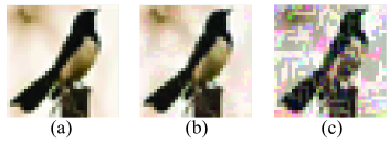
Figure 2: To launch a valid attack from an input image (a), the adversarial example (b) must be perceptually similar to the original image (e.g., here $\Delta=0.031$). Otherwise, it can be easily pinpointed. In our method, the transformed image is used for training $f_{a}$, not attacking. We therefore intentionally add much stronger adversarial noise to the input (c) (here $\Delta=0.2$). The strong noise helps to strengthen the robustness of $f_{a}$ and defend against BPDA attacks (see Sec. 3.3).

Embracing adversarial noise.

Given an input image $\bm{x}$, our adversarial transformation effectively adds perturbation noise to $\bm{x}$. The perturbation range $\Delta$ controls how much noise is added. Normally, in adversarial attacks, $\Delta$ is set small to generate adversarial examples perceptually similar to the input image. But when we use adversarial attacks (on $f_{b}$) as a means of input transformation for training $f_{a}$, we have the freedom to use a much larger $\Delta$, thereby adding noticeably stronger adversarial noise (see Fig. 2-c).

At training time, the excessively strong adversarial noise forces the network $f_{a}$ to learn how to classify robustly. This is because perturbations crafted on an external model can approximate the adversarial examples of the model under training (an insight inspired the prior work [44]). This reason, although valid, can not explain how our method is able to avoid the deficiencies of prior defense methods. There exist deeper reasons:

Randomness.

The adversarial noise added by our $g(\bm{x})$ is randomized, since the update rule (3) always starts from the input image with a random perturbation (i.e., $\bm{x}+\bm{\delta}$ with uniformly sampled $\bm{\delta}_{i}\sim[-\Delta,\Delta]$). Randomization is not new; prior defenses also employ randomized transformations to the input. But they have been circumvented by Expectation Over Transformation (EOT)  [2, 3]. EOT attack first estimates the gradient of expected $f(g(\bm{x}))$ with respect to $\bm{x}$ using the relationship $\nabla\operatorname*{{\mathbb{E}}}_{\tilde{g}\sim\mathcal{T}}f(\tilde{g}(\bm{x}))=\operatorname*{{\mathbb{E}}}_{\tilde{g}\sim\mathcal{T}}\nabla f(\tilde{g}(\bm{x}))$, where $\tilde{g}(\cdot)$ is a deterministic version of $g(\cdot)$ sampled from the distribution of randomized transformations $\mathcal{T}$. It then uses the estimated gradients in PGD-type attacks to generate adversarial examples. Thus, the feasibility of EOT hinges on a reliable estimation of $\nabla f(\tilde{g}(\bm{x}))$. In our method, $\tilde{g}(\bm{x})$ corresponds to solving the optimization problem (2) starting from a particular sample $\bm{x}+\bm{\delta}$.

In what follows, we examine a range of strategies that have been successfully used to estimate $\nabla f(\tilde{g}(\bm{x}))$ in prior defense methods (and thus break them), and show that our method is robust against all those attacking strategies.

Automatic differentiation.

By chain rule, the estimation of $\nabla f(\tilde{g}(\bm{x}))$ requires the knowledge of $\tilde{g}(\bm{x})$’s Jacobian (first-order derivatives) $\text{D}\tilde{g}(\bm{x})$. A straightforward attempt to this end is by unrolling the iterative steps (3) and using automatic differentiation (AD) [47] to compute $\text{D}\tilde{g}(\bm{x})$. Yet, this is infeasible. As shown in (3), the iterative steps involves non-differentiable operators including $\text{sgn}(\cdot)$ and $\Pi_{\bm{x}^{\prime}\in\Delta_{\bm{x}}}[\cdot]$. Thus, directly applying AD leads to erroneous estimation of $\text{D}\tilde{g}(\bm{x})$, which in turn obstructs the search for adversarial examples. Our early experiments indeed show that virtually no adversarial examples crafted using AD can fool our model.

Backward Pass Differentiable Approximation (BPDA).

To circumvent the defense using non-differentiable operators, Athalye et al. [2] introduced a strategy called Backward Pass Differentiable Approximation (BPDA) to estimate the defense model’s gradients. The idea is to replace the non-differentiable operators in $\tilde{g}$ with differentiable approximations, and estimate the derivatives $\text{D}\tilde{g}(\bm{x})$ in AD by computing the AD’s forward pass using the original $\tilde{g}$ and computing its backward pass using $\tilde{g}$’s differentiable approximation. BPDA has succeed in gradient-based attacks (such as PGD and C&W [8]) toward many prior defenses, allowing the adversary to craft efficient adversarial examples.

When applying BPDA to estimate the gradients of our defense model, we replace $\text{sgn}(\cdot)$ and $\Pi_{\bm{x}^{\prime}\in\Delta_{\bm{x}}}[\cdot]$ in (3) with their differentiable approximations (see Sec. 4.1 for details). We found that if the number of iterations (LL-PGD steps) for applying (3) is low (i.e., $\leq 2$), BPDA indeed enables the adversary to find valid adversarial examples. But when the number of iterations is set moderately high (i.e., $>4$), BPDA is greatly thwarted; the adversary can hardly find any valid adversarial example (see Sec. 4.1). This is because the differentiable approximations must be applied in each iteration, and as the number of iterations increases, the approximation error accumulates rapidly.

Finite difference gradients.

Another strategy for estimating $\text{D}\tilde{g}(\bm{x})$ is the classic finite difference estimation. Each element in the Jacobian matrix $\text{D}\tilde{g}(\bm{x})$ can be estimated using

$$\frac{\partial\tilde{g}_{i}(\bm{x})}{\partial\bm{x}_{j}}\approx\frac{1}{2h}\left[\tilde{g}_{i}(\bm{x}+\bm{h}_{j})-\tilde{g}_{i}(\bm{x}-\bm{h}_{j})\right],$$ (4)

where $\tilde{g}_{i}(\bm{x})$ indicates the $i$-th element (or pixel) of the transformed image, and $\bm{h}_{j}$ is a vector with all zeros except the $j$-th element (or pixel) which has a value $h$.

Our defense inherently thwarts this attacking strategy. It causes the adversary to suffer from either exploding or vanishing gradients [2]. Figure 3-left shows a 1D depiction illustrating this phenomenon in our method. Indeed, our experiments confirm that it is too unreliable to estimate derivatives using (4) (see Fig. 3-right).

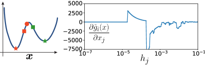
Figure 3: (left) We show a 1D depiction of our input transformation $g(\bm{x})$, the process aiming to find the local minimum of the optimization problem (2). Starting from an $\bm{x}_{0}$ at the red dot, $g(\bm{x})$ will reach a position at the red star. Perturbing $\bm{x}_{0}$ toward one side (to the red square), $g(\bm{x})$ will still reach the red star, and in this way, the finite difference gradient vanishes. But if $\bm{x}_{0}$ is perturbed to the green square, $g(\bm{x})$ will reach the green star—an entirely different local minimum, and the finite difference gradient explodes. (right) We plot $\frac{\partial\tilde{g}_{i}(\bm{x})}{\partial\bm{x}_{j}}$ (for particular $i$ and $j$ here) estimated by finite difference method (4) with an increasing $h_{j}$. When $h_{j}$ is extremely small ($<10^{-5}$), the estimated gradient vanishes; as $h_{j}$ increases, the estimated gradient fluctuates severely, due to the reason illustrated on the left.

Reparameterization.

Vanishing and exploding gradients have been exploited as a defense mechanism [39, 33]. Yet those defenses have been proven vulnerable under a reparameterization strategy [2]. This strategy aims to find some differentiable function $h(\cdot)$ for a change-of-variable $\bm{x}=h(\bm{z})$ such that $\tilde{g}(h(\bm{z}))\approx h(\bm{z})$. If such a function $h(\cdot)$ can be found, then one can compute the gradient of the differentiable function $f(h(\bm{z}))$ to launch adversarial attack.

To break our defense using this strategy, one must find an $h(\cdot)$ that constructs the adversarial examples of $f_{b}$ directly (so that $\tilde{g}(h(\cdot))=h(\cdot)$), without solving the optimization problem (2). We argue that finding such an $h(\cdot)$ is extremely hard. If $h(\cdot)$ could be constructed, we would have a direct way of crafting adversarial examples; PGD-type iterations would not be needed; and the entire territory of adversarial learning would be redefined—which are unlikely to happen.

Indeed, we implemented this strategy by training a neural network model $h_{\bm{\theta}}$ that aims to minimize $\|h_{\bm{\theta}}(\bm{x})-\tilde{g}(\bm{x})\|_{2}$ over the natural image distribution. This attempt is futile. Our experiments show that the generalization error of the trained $h_{\bm{\theta}}$ is too high to launch any valid adversarial attack (see Appendix A.2). This conclusion also echos the prior studies [4, 48], which show that learning-based adversarial attacks usually perform worse than gradient-based attacks.

Identity mapping approximation.

Some prior defense methods also use an optimization process to transform the input image—for example, the optimization that aims to erase adversarial noise from the input image [14, 33]. In those defenses, the transformed image $g(\bm{x})$ remain similar to the input $\bm{x}$. Consequently, as shown in [2], those defenses can be easily circumvented by replacing $g(\cdot)$ with the identity mapping in the backward pass of BPDA attack.

Similarly, in our defense, if the perturbation range $\Delta$ in (3) for defining $g(\cdot)$ were set small, $g(\bm{x})$ (the adversarial example of $f_{b}$) would be close to $\bm{x}$, and our defense would be at risk. To prevent this vulnerability, we must ensure that $g(\cdot)$ be far from the identity mapping. This requires us to set a relatively large $\Delta$. In practice, we use $\Delta=0.2$ for pixel values ranging in $[0,1]$ (see details in Sec. 4.1).

It turns out that a relatively large $\Delta$ is necessary but not sufficient. The choice of the network model $f_{b}$ also affects how far $g(\bm{x})$ is from $\bm{x}$ statistically, as we will discuss next.

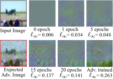
Figure 4: We apply the adversarial transformation $g(\cdot)$ defined on different models $f_{b}$ to an input image (top-left). Corresponding to the six images toward the right are the $f_{b}$ models (with the same network structure) untrained, trained with an increasing number of epochs, and adversarially trained. In each of those six images, we visualize the normalized difference between the input $\bm{x}$ and the expectation over transformation (EOT) image $\operatorname*{{\mathbb{E}}}_{\tilde{g}\sim\mathcal{T}}\tilde{g}(\bm{x})$ (estimated using 5000 samples). The $L_{\infty}$ norms of the difference images are shown under the images. Image in the red box (bottom-left) is the EOT image $\operatorname*{{\mathbb{E}}}_{\tilde{g}\sim\mathcal{T}}\tilde{g}(\bm{x})$ produced using an adversarially trained $f_{b}$ model. Because we intentionally use a large perturbation range $\Delta=0.2$, this image has pronounced artifacts.

3.4 Choosing Pre-trained Model $\bm{f_{b}}$

A large perturbation range $\Delta$ allows our adversarial transformation $g(\cdot)$ to output an image far from the input. Yet, because of the randomness in $g(\cdot)$, a large $\Delta_{\bm{x}}$ can not guarantee that $g(\bm{x})$ is statistically different from $\bm{x}$. If the expectation over the transformation $\operatorname*{{\mathbb{E}}}_{\tilde{g}\sim\mathcal{T}}\tilde{g}(\bm{x})$ remains close to $\bm{x}$, our defense method may still suffer from the aforementioned BPDA attack, in which identity mapping can be used to approximate $g(\cdot)$ in the backward pass.

	Untrained	1 epoch	2 epochs	5 epochs	10 epochs	15 epochs	20 epochs	Adv. trained
Standard Acc.	81.8%	81.6%	82.4%	83.0%	82.4%	82.2%	82.7%	82.9%
BPDA-I Acc.	30.6%	30.7%	40.0%	46.4%	62.3%	63.1%	62.9%	80.5%
Avg. $L_{\infty}$ dist.	0.005	0.033	0.036	0.067	0.130	0.133	0.136	0.272

Table 1: Discovery for choosing $f_{b}$. Corresponding to individual columns are $f_{b}$ models untrained, trained with an increasing number of epochs, and adversarially trained. For the defense model $f_{a}(g(\cdot))$ equipped with each $f_{b}$, we evaluate its standard accuracy (first row) and robust accuracy (second row) under the BPDA-I attack (see Sec. 4.1). The third row shows $\|\bm{x}-\operatorname*{{\mathbb{E}}}_{\tilde{g}\sim\mathcal{T}}\tilde{g}(\bm{x})\|_{\infty}$ where $\operatorname*{{\mathbb{E}}}_{\tilde{g}\sim\mathcal{T}}\tilde{g}(\bm{x})$ is estimated using 5000 samples. Notice the correlation between the increase of the $L_{\infty}$ distance and the increase of adversarial robustness.

This intuition is supported by an empirical discovery. We experimented with an input transformation ${g}(\cdot)$ constructed using an untrained model $\bar{f}_{b}$ whose weights are assigned randomly. As shown in Fig. 4 and the first column in Table 1, the expectation over transformation $\operatorname*{{\mathbb{E}}}_{\tilde{g}\sim\mathcal{T}}\tilde{g}(\bm{x})$ is indeed close to $\bm{x}$ (in $L_{\infty}$ norm), and the BPDA attack with identity mapping approximation can easily fool this defense model.

Next, we train a series of models $f^{(i)}_{b}$, each obtained with an increasing number of training epochs. We found that as the number of training epochs increases, the expectation over transformation $\operatorname*{{\mathbb{E}}}_{\tilde{g}\sim\mathcal{T}}\tilde{g}(\bm{x})$ resulted by using each of these $f^{(i)}_{b}$ models drifts further away from $\bm{x}$, that is, $\|\bm{x}-\operatorname*{{\mathbb{E}}}_{\tilde{g}\sim\mathcal{T}}\tilde{g}(\bm{x})\|_{\infty}$ increases. Meanwhile, the defense model $f(g(\cdot))$ trained with the corresponding $f^{(i)}_{b}$ becomes more robust, yielding increasingly better robust accuracy under the BPDA attack (see Table 1).

Remarkably, we discover that an even larger distance $\|\bm{x}-\operatorname*{{\mathbb{E}}}_{\tilde{g}\sim\mathcal{T}}\tilde{g}(\bm{x})\|_{\infty}$ can be obtained, if the model $f_{b}$ is adversarially trained. When used in $g(\cdot)$, the adversarially trained model $f_{b}$ further improves the robustness of our defense model. This discovery confirms our intuition.

Computational performance.

The choice of $f_{b}$ also affects the computational cost of our defense method. A complex network structure of $f_{b}$ makes $g(\cdot)$ expensive, which in turn imposes a large performance overhead on both the training of $f_{a}$ and the inference using $f_{a}$. Therefore, a simple network structure is preferred.

The freedom of choosing a simple network $f_{b}$ brings our method a performance advantage over adversarial training. In adversarial training, adversarial examples are crafted on the classification network $f_{a}$ for each input image at every epoch. In our training, however, by choosing a model $f_{b}$ simpler than $f_{a}$, it becomes faster to find adversarial examples. As shown in our experiments (in Sec. 5), in comparison to adversarial training, our defense requires shorter training time, and at the same time offers stronger robustness.

Guiding rules.

In summary, we present two guiding rules for choosing $f_{b}$. 1) $f_{b}$ should be chosen to yield a large $\|\bm{x}-\operatorname*{{\mathbb{E}}}_{\tilde{g}\sim\mathcal{T}}\tilde{g}(\bm{x})\|_{\infty}$ value. Given an $f_{b}$’s network structure, adversarial training on $f_{b}$ (in pre-training step) is preferred. 2) Meanwhile, the structure of $f_{b}$ should be as simple as possible. In Appendix A.1, we report $f_{b}$’s network structure that we use in our experiments.

4 Devil’s Advocate

We now play devil’s advocate in attacking our defense method. In our defense, the network gradient with respect to the input (i.e., $\nabla f_{a}(g(\bm{x}))$) is intentionally undefined. Thus one can not craft adversarial examples by directly applying PGD-type methods on our defense (recall Sec. 2). We therefore evaluate our defense against a range of other possible attacks, including those discussed in Sec. 3.3. Later in Sec. 5, we will compare the worst-case robustness of our defense under these attacks with various recently proposed defense methods.

Common experiment setups.

Experiments in this section are conducted on CIFAR-10 dataset [18] with standard training/test split. We use ResNet18 [15] as the classification model $f_{a}$ and a small VGG-style network for $f_{b}$, whose details are given in Appendix A.1. All models are trained for 80 epochs using Stochastic Gradient Descent (SGD) (constant learning rate=0.1, momentum=0.9). Our adversarial transformation $g(\cdot)$ performs LL-PGD update (3) for 13 iterations, each with a stepsize $\epsilon=\Delta/6$. The perturbation range $\Delta$ varies in individual experiments, and will be reported therein.

Metric.

Following prior work, our evaluation uses an accuracy measure defined as the ratio of the number of correctly classified images to the total number of tested images. We refer to this measure as standard accuracy if the tested images include only clean images, and as robust accuracy if the tested images consist of adversarially crafted images.

4.1 BPDA Attack and the Variants

BPDA attack [2], as reviewed in Sec. 3.3, is a powerful way to estimate network gradients that are obfuscated by defense methods. The estimated gradients are then used in PGD-type methods (if the defense is deterministic) or the EOT method (if the defense is randomized) for crafting adversarial examples. BPDA has circumvented a handful of recent defense techniques [14, 50, 25, 39, 7] that implement gradient obfuscation, in many defenses resulting in 0% robust accuracy. We therefore evaluate our defense against it and its possible variants.

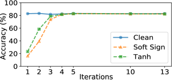
Figure 5: Robustness under BPDA. We evaluate the robust accuracy of our defense under two versions of BPDA attacks, which replace $\text{sgn}(\cdot)$ in (3) with soft sign (in orange) and tanh (in green), respectively. The resulting two robust accuracies are compared with our defense model’s standard accuracy (in blue) evaluated with clean (natural) images. Along X-axis, we repeat this evaluation, each time with an increasing number of LL-PGD steps (3) in our adversarial transformation $g(\cdot)$. To highlight only the effect of the smooth approximations of $\text{sgn}(\cdot)$ and $\Pi_{\bm{x}^{\prime}\in\Delta_{\bm{x}}}(\cdot)$, we factor out the randomness in our defense by disabling the random start at the beginning of (3). After the network gradient is estimated using BPDA, we use PGD to search for adversarial examples with a maximum perturbation size of 0.031 (in $L_{\infty}$ norm). The PGD search takes 50 iterations with a stepsize 0.002.

Differentiable approximation on backward pass.

The update rule (3) in our adversarial transformation involves two non-differentiable operators, namely, $\textrm{sgn}(\cdot)$ and $\Pi_{\bm{x}^{\prime}\in\Delta_{\bm{x}}}(\cdot)$, whose specific forms are given in Appendix A.3. To launch BPDA attack, we need to replace them with differentiable operators and compute their derivatives. We experimented with two different smooth approximations of $\textrm{sgn}(\cdot)$: the soft sign function $\frac{x}{1+|x|}$ and tanh function $\frac{e^{x}-e^{-x}}{e^{x}+e^{-x}}$. The smooth approximation of $\Pi_{\bm{x}^{\prime}\in\Delta_{\bm{x}}}(\cdot)$ is not explicitly defined. Instead, we directly approximate its derivative using

$$\frac{\text{d}}{\text{d}x}\Pi_{\bm{x}^{\prime}\in\Delta_{\bm{x}}}(x)\approx\begin{cases}1,&\text{if}\ |x|<\Delta,\\ \frac{1}{(1+|x|)^{2}},&\text{otherwise.}\end{cases}$$ (5)

Reported in Fig. 5, the experiments show that our defense is robust to this attack, as long as the number of LL-PGD steps $N$ in $g(\cdot)$ is not too small (i.e., $N>5$).

If the number of LL-PGD steps $N$ is set too small, BPDA attack is indeed able to find adversarial examples (Fig. 5). Therefore, another attempt one may ponder is to craft adversarial examples on a model trained with a small $N$ ($N\leq 3$), and use them to transfer attack our defense (which is trained with a larger $N$). This attack remains ineffective (see details in Appendix A.3). We conjecture that this is because the adversarial examples for the model with a small $N$ have a different distribution from that with a larger $N$ [30, 40].

Identity mapping approximation.

Another possible attack is by replacing the input transformation $g(\cdot)$ with the identity mapping for gradient estimation in BPDA backward pass (recall discussion in Sec. 3.3). We refer this attack as BPDA-I attack. Under this attack, several previous defenses (e.g., [33, 39, 14]) have been nullified.

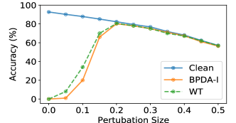
Figure 6: Robustness w.r.t. perturbation size. We test our defense robustness using independently trained defense models with increasing perturbation range $\Delta$ used in $g(\cdot)$. The standard accuracy (blue curve) is measured using clean images. The robust accuracies under BPDA-I attack (Sec. 4.1) and WT attack (Sec. 4.2) are in orange and green, respectively. In our input transformation, we enable random start of (3). Therefore, in BPDA-I attack, we use 500 samples of $\tilde{g}(\cdot)$ for EOT gradient estimation. The gradient-descent setup is the same as that in the earlier experiments in Fig. 5.

We applied BPDA-I attack on our defense. The attack setup and results are summarized in Fig. 6. As the perturbation size $\Delta$ in the adversarial transformation increases, the robust accuracy of our method increases. The robust accuracy is always upper bounded by the standard accuracy, which decreases gradually as $\Delta$ increases. If $\Delta$ is too large, the excessive perturbations to the input make the network $f_{a}$ harder to learn and thus lower the standard and robust accuracies. Empirically, $\Delta=0.2$ offers the best performance.

Reparameterization.

In Sec. 3.3, we described another BPDA strategy, one that uses reparameterization to smoothly approximate our adversarial transformation $g(\cdot)$. As discussed therein, it is extremely hard to directly derive the reparameterization function. Instead, we attempted to train a Fully Convolutional Network [24] to represent $h(\bm{z})$. We denote this network as $h(\bm{x};\bm{\theta})$, whose weights are optimized with the loss function, $\ell(\bm{\theta})=\operatorname*{{\mathbb{E}}}_{\bm{x}\in\mathcal{X}}\left\lVert h(\bm{x};\bm{\theta})-g(\bm{x})\right\rVert^{2}.$ Here $\mathcal{X}$ represents the distribution of natural images (we use CIFAR-10 as the training dataset).

Our experiment shows that although we can reach a low loss value in training $h(\bm{x};\bm{\theta})$, the loss on test dataset always stays high, indicating that $h(\bm{x};\bm{\theta})$ is always overfitted. As a result, the adversarial examples resulted in this way have almost no effect on our defense model—the accuracy drop under this attack is within 1% from the standard accuracy. See Appendix A.2 for the details of this experiment.

4.2 Gradient-Free Attacks

Several attacking methods require no gradient information of the model, and they can be employed to potentially threaten our defense. As discussed in Sec. 2, these attacks fall into two categories: transfer attack and query-based attack. Against both types of attacks we evaluate our defense.

White-box transfer attack.

In white-box setting, the adversary has full knowledge of our defense model. A tempting idea is to generate adversarial examples on the classifier model $f_{a}$, and use them to transfer attack our defense model $f_{a}(g(\cdot))$. Note that this differs from BPDA-I attack in Sec. 4.1, where $f_{a}$ is used only in the backward pass for gradient estimation while the forward pass still uses the full model $f_{a}(g(\cdot))$. Here, in contrast, adversarial examples are generated solely on $f_{a}$. We refer this attack as White-box Transfer (WT) attack, and report the robust accuracies of our defense in Fig. 6, along with the results under BPDA-I attack. We found that our model’s robustness performances under both attacks are similar, and $\Delta=0.2$ is the best choice.

One may realize another attacking possibility by noticing the way we choose $f_{b}$ (on which we perform adversarial transformation). In Sec. 3.4, we present that $f_{b}$ should be chosen such that for a given natural image $\bm{x}$ the average transformation $\operatorname*{{\mathbb{E}}}_{\tilde{g}\sim\mathcal{T}}\tilde{g}(\bm{x})$ stays far from $\bm{x}$. Thus, it seems plausible to first generate adversarial examples on $f_{a}$ using PGD attack starting from the average transformation $\operatorname*{{\mathbb{E}}}_{\tilde{g}\sim\mathcal{T}}\tilde{g}(\bm{x})$, and use them to attack our full model $f_{a}(g(\cdot))$. However, thanks to the large perturbation range $\Delta_{\bm{x}}$ we use (recall Sec. 3.3), $\operatorname*{{\mathbb{E}}}_{\tilde{g}\sim\mathcal{T}}\tilde{g}(\bm{x})$ is always far from a natural image (see the image in the red box of Fig. 4). Thus the adversarial examples generated in this way all have easily noticeable artifacts; they are not valid.

Defense Model	Clean	Transfer	HSJ	GA
No defense	92.9%	1.3%	3.6%	5.8%
Madry et al. [26]	81.7%	77.5%	72.1%	78.4%
Ours	82.9%	78.1%	82.0%	81.9%

Table 2: Robustness under black-box attacks. In the transfer attack, adversarial examples are crafted on an independently trained ResNet18 model. The query-based attacks are performed using a third-party library foolbox [32] with default parameters to launch these attacks. All adversarial examples are restricted in the $L_{\infty}$ ball with a perturbation size of $0.031$.

Black-box attacks.

We also evaluate our defense against the black-box attacks, including the black-box transfer attack [30] and two most recently introduced query-based attacks, HopSkipJumpAttack (HSJ) [9] and GenAttack (GA) [1]. In Table 2, we summarize the robust accuracies of our model under these attacks, along with two baselines from the same classification model ($f_{a}$) optimized respectively using standard training and adversarial training.

5 Comparisons and Further Evaluation

Comparisons.

We now compare the robustness of our method with other state-of-the-art defense methods under white-box attacks. Unlike many others that can be attacked using PGD-type methods, our defense model is inherently non-differentiable, immune to direct PGD attacks. Therefore it is not possible to compare all these defense methods under exactly the same attacks. Instead, we compare the worst-case robustness of our method under all the attacks described in Sec. 4 with other methods.

Method	$A_{std}$	$A_{rob}$	Best Attack
No defense	92.9%	0.0%	PGD
Madry et al. [26]	81.7%	42.7%	PGD
Zhang et al. [54]	80.4%	44.6%	PGD
Xie et al. [51]	83.8%	45.2%	PGD
Guo et al.* [14]	-	0.0%	BPDA
Buckman et al.* [7]	-	0.0%	BPDA
Dhillon et al.* [10]	-	0.0%	BPDA
Song et al.* [39]	-	5.0%	BPDA
Ours (under BPDA)	82.9%	80.2%	BPDA
Ours	82.9%	78.1%	Transfer

Table 3: Comparisons on CIFAR-10. Methods indicated by * are those circumvented in [2]. We evaluate other methods using the code provided in the original papers, training them using the same network and hyperparameters as our method. The perturbation range of all adversarial examples is $\Delta=0.031$. The last column indicates the most efficient attacking method that produces the worst robustness. The second last row indicates the worst-case robustness of our method under all BPDA-type attacks, while the last row indicates our worst-case robustness under all attacks.

The comparison results on CIFAR-10 dataset are summarized in Table 3, where $A_{std}$ is the standard accuracy tested with clean images, and $A_{rob}$ is the worst-case robust accuracy under all tested attacks. The methods indicated by a star (*) are those circumvented by Athalye et al. [2]. We include their results therein as a reference. The other defense methods (including ours) all use ResNet18 as their classification model, trained with SGD (learning rate=0.1, momentum=0.9) for 80 epochs.

On CIFAR-10 dataset, the most effective attack on our method is the black-box transfer attack (Sec. 4.2), although its severity surpasses BPDA attacks only slightly: the worst-case robust accuracy of our method under BPDA attack and its variants (Sec. 4.1) is 80.2%. Nevertheless, our robustness performance is significantly better than the state-of-the-art methods, as shown in Table 3.

We also performed the comparisons on Tiny ImageNet dataset, and our method demonstrates significantly stronger robustness as well. In short, our worst-case robust accuracy is 40.2%, in stark contrast to previous methods, which all have robust accuracies around 18%. The results are reported in details in Appendix A.4.

Training cost.

Our method has significantly lower training cost than the adversarial training [26, 54, 51], while offering stronger robustness. For example, our method takes 82 minutes to train a ResNet18 model on CIFAR-10 for 80 epochs, while the adversarial training takes 460 minutes. As a baseline, the standard training takes 56 minutes. All timings are measured on a NVIDIA RTX 2080Ti GPU.

Sufficiency of EOT samples.

Our defense is randomized, and when using EOT to attack our method we take 500 samples of $\tilde{g}(\cdot)$ (recall experiments in Fig. 6). Here we conduct additional experiments to ensure the sufficiency of using 500 samples for estimating the expectation. As shown in Fig. 7, when the perturbation size $\Delta$ is small and the number of samples is also small (e.g., $<100$), increasing sample size indeed allows EOT to better attack our method. However, when the perturbation size is set to 0.2, the value we consistently use throughout all our evaluations, EOT attacks became persistently inefficient, regardless of the sample size. Therefore, we conclude that 500 samples in EOT allow thorough evaluation of our defense against EOT.

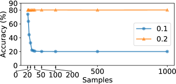
Figure 7: Robustness w.r.t. EOT samples. When using EOT to attack our method, we sample our adversarial transformation with different random starts $\bm{x}+\bm{\delta}$ to estimate the expected $\nabla f_{a}(g(\bm{x}))$. When $\Delta=0.1$ (blue curve), increasing the sample size allows EOT to better attack our defense, until it plateaus. But when $\Delta=0.2$ (orange curve), EOT becomes persistently inefficient.

6 Conclusion

We have presented a simple defense mechanism against adversarial attacks. Our method takes advantage of the numerical recipe that searches for adversarial examples, and turns this harmful process into a useful input transformation for better robustness of a network model. On CIFAR-10 and Tiny ImageNet datasets, it demonstrates state-of-the-art worst-case robustness under a wide range of attacks. We hope our work can offer other researchers a new perspective to study the adversarial defense mechanisms. In the future, we would like to better understand the theoretical properties of our adversarial transformation and their connections to stronger adversarial robustness.

Supplementary Document
One Man’s Trash is Another Man’s Treasure:
Resisting Adversarial Examples by Adversarial Examples

Appendix A Additional Experiments and Setups

A.1 Network Structure of $\bm{f_{b}}$

Following the guidelines presented at the end of Sec. 3.4, we choose to use a VGG-style small network in $f_{b}$ for defining our adversarial transformation. This network is simple enough to enable fast adversarial transformation, while producing the expectation over transformation image (i.e., $\operatorname*{{\mathbb{E}}}_{\tilde{g}\sim\mathcal{T}}\tilde{g}(\bm{x})$) drastically different from the input image. The structure of $f_{b}$ for experiments on CIFAR-10 dataset is described in Table 4.

On Tiny ImageNet dataset, the network structure of $f_{b}$ remains largely the same except two minor changes to accommodate the different resolution of the images in Tiny ImageNet. Namely, the changes are at the 12nd layer (which has a dimension 2048) and the 15th layer (which has a dimension 200).

Layer	Module	Output Size
1	Input	3$\times$32$\times$32
2	Conv(k=3), BN, ReLU	64$\times$32$\times$32
3	MaxPool	64$\times$16$\times$16
4	Conv(k=3), BN, ReLU	128$\times$16$\times$16
5	MaxPool	128$\times$8$\times$8
6	Conv(k=3), BN, ReLU	128$\times$8$\times$8
7	Conv(k=3), BN, ReLU	128$\times$8$\times$8
8	MaxPool	128$\times$4$\times$4
9	Conv(k=3), BN, ReLU	128$\times$4$\times$4
10	Conv(k=3), BN, ReLU	128$\times$4$\times$4
11	MaxPool	128$\times$2$\times$2
12	Flatten	512
13	Linear, ReLU, Dropout	512
14	Linear, ReLU, Dropout	512
15	Linear (output)	10

Table 4: Network structure for $f_{b}$. Here BN denotes batchnorm operation, and Conv(k=3) denotes convolutional layer with a kernel size of 3.

A.2 Reparameterization Attack

As discussed in Sec. 3.3 and 4.1, to launch the reparameterization attack, we need to find a forward function $h(\cdot)$ that approximate our adversarial transformation process. To this end, we attempted to train a Fully Convlutional Network (FCN) [24], denoted as $h(\bm{x};\bm{\theta})$, through the following optimization,

$$\bm{\theta}=\operatorname*{arg\,min}_{\bm{\theta}}\mathbb{E}_{\bm{x}\in\mathcal{X},\bm{\delta}\in\bm{\Delta}}\left\lVert h(\bm{x}+\bm{\delta};\bm{\theta})-\tilde{g}_{\bm{\delta}}(\bm{x})\right\rVert^{2},$$ (6)

where $\mathcal{X}$ is the given dataset, $\bm{\delta}$ is the initial input perturbation in the $L_{\infty}$ ball of size $\Delta$ (as described in Sec. 3.3), $\tilde{g}_{\bm{\delta}}(\cdot)$ is the deterministic version of our adversarial transformation $g(\cdot)$: it starts the adversarial search iteration (3) from $\bm{x}+\bm{\delta}$ by using a sampled $\bm{\delta}$.

However, after optimizing (6), we found that although the FCN model can reach a relatively low training error, the error on test set remains high, as depicted in Fig. 8. This suggests that the FCN model is not able to learn a $h(\bm{x};\bm{\theta})$ that generalizes well. The inability to generalize is not a surprise: if $h(\bm{x};\bm{\theta})$ could generalize well, we would have a direct way of crafting adversarial examples; and PGD-type iterations would not be needed—which are all unlikely.

Indeed, when we use the trained $h(\bm{x},\bm{\theta})$ to launch a reparameterization attack to our model, the attack hardly succeeds. Under this attack (on CIFAR-10), the robust accuracy of our defense is 81.1%, even better than the robust accuracy under BPDA-I attack (80.2%). In fact, this accuracy nearly reaches its upper bound, the standard accuracy (i.e., 82.9%), as reported in Table 3 of the main text.

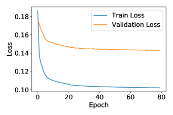
Figure 8: Training Loss and validation loss in reparameterization attack.

		Robust Acc. (transfer attack)
Defense Model Iterations	Standard Acc.	$N=1$	$N=2$	$N=3$
$N=3$	81.7%	69.7%	66.4%	79.5%
$N=4$	82.4%	75.6%	78.7%	79.9%
$N=5$	83.1%	81.6%	80.7%	81.7%
$N=10$	82.7%	81.4%	81.2%	81.0%
$N=13$	82.9%	80.9%	81.1%	81.3%

Table 5: Transfer attack based on BPDA. Each row shows the standard and robust accuracies of our defense model with a different number of LL-PGD steps in its adversarial transformation $g(\cdot)$. The number of LL-PGD steps in our defense model is shown in the left most column. The right most three columns correspond to the models with smaller numbers of LL-PGD steps. We use these models to craft adversarial examples to transfer attack our defense model. It shows that even when the number $N$ of LL-PGD steps in our defense model is moderately large ($N\geq 5$), the transfer attacks become ineffective. In all the evaluations, the perturbation size $\Delta$ in our defense model is set as $\Delta=0.2$.

A.3 BPDA Attack Details and Additional Results

As described in Sec. 4.1, we evaluate our defense model under the BPDA attack. To launch BPDA attack, we need to replace the non-differentiable operators in our adversarial transformation with their smooth approximations. In particular, the non-differentiable operators in the adversarial update rule (3) (in the main text) are the $\textrm{sgn}(\cdot)$ function,

$$\text{sgn}(\bm{x})=\begin{cases}1&\text{if}\ \bm{x}>0,\\ 0,&\text{if}\ \bm{x}=0,\\ -1&\text{if}\ \bm{x}<0.\end{cases}$$ (7)

and the $L_{\infty}$ projection operator,

$$\Pi_{\bm{x}^{\prime}\in\Delta_{\bm{x}}}(\bm{x})=\begin{cases}\bm{x}&\text{if}\ |\bm{x}|\leq\Delta,\\ -\Delta&\text{if}\ \bm{x}<-\Delta,\\ \Delta&\text{if}\ \bm{x}>\Delta.\end{cases}$$ (8)

In Sec. 4.1, we experimented with two different smooth approximations of the $\textrm{sgn}(\cdot)$ function, namely, the soft sign function $\frac{x}{1+|x|}$ and tanh function $\frac{e^{x}-e^{-x}}{e^{x}+e^{-x}}$, and the projection operator is replaced by directly approximating its derivative using (5).

Also discussed in Sec. 4.1 is an additional transfer attack: First, we craft adversarial examples by setting the number $N$ of LL-PGD steps to be a small value. This is motivated by the observation that, as shown in Fig. 5, BPDA attack is able to find effective adversarial examples when $N$ is small. We then use the resulting adversarial examples to transfer attack our defense model, which uses a larger number of LL-PGD steps in the adversarial transformation (in both training and inference). As summarized in Table 5, our experiment shows that this attack remains ineffective to our defense.

Method	$A_{std}$	$R_{rob}$	Best Attack
No defense	58.2%	0.0%	PGD
Madry et al. [26]	42.7%	17.3%	PGD
Zhang et al. [54]	40.6%	17.7%	PGD
Mao et al. [27]	40.9%	17.5%	PGD
Ours (Under BPDA)	48.8%	47.9%	BPDA
Ours	48.8%	40.2%	Transfer

Table 6: Comparisons on Tiny ImageNet. The layout of this table is similar to Table 3 in the main text (i.e., the comparisons on CIFAR-10). The perturbation range of all adversarial examples is $\Delta=0.031$. The last column indicates the most efficient attacking method that produces the worst robustness. The second last row indicates the worst-case robustness of our method under all BPDA-type attacks, while the last row indicates our worst-case robustness under all attacks.

A.4 Evaluation on Tiny ImageNet

We also evaluate our defense model on Tiny ImageNet dataset consisting of 64px$\times$64px RGB images. These images fall into 200 classes, each has 500 images for training and 50 images for testing. Following the evaluations setups in prior works, the adversarial examples used in the attacks have a maximum perturbation size (in $L_{\infty}$ norm) of 0.031 for pixel values ranging in [0,1]. We use ResNet18 as our classification network (in $f_{a}$) and the network structure of $f_{b}$ is described in Appendix A.1.

We compare our method with the state-of-the-art method [27] evaluated on Tiny ImageNet and the methods based on adversarial training [26, 54]. For all those methods, we use the implementation code provided in their original papers. When comparing with these methods, we use the same training protocol: the models are optimized use SGD (learning rate=0.1, momentum=0.9) and trained for 80 epochs.

As shown in Table 6, our method demonstrates significantly stronger robustness in comparison to previous methods. Our worst-case robust accuracy is 40.2%. In contrast, previous methods have robust accuracies around 18%. Remarkably, the standard accuracy of our method also outperforms previous methods.

A.5 Expectation over Transformation Images

Figure 4 in the main text shows a few examples of the difference between an input image $\bm{x}$ and its expectation over transformation, that is, the image of normalized $\bm{x}-\operatorname*{{\mathbb{E}}}_{\tilde{g}\sim\mathcal{T}}\tilde{g}(\bm{x})$. We now provide more samples of $\bm{x}-\operatorname*{{\mathbb{E}}}_{\tilde{g}\sim\mathcal{T}}\tilde{g}(\bm{x})$ images on both CIFAR-10 and Tiny ImageNet (see Fig. 9).

Discussion.  In [45], Tsipras et al. presented an interesting finding. They visualized the loss gradient with respect to input pixels, and found that if the model is adversarially trained, such a loss gradient is significantly human-aligned—they align well with perceptually relevant features (e.g., see Figure 2 in their paper). But if the model is not adversarially trained, the loss gradient appears like random noise. Here, we discover that the normalized difference $\bm{x}-\operatorname*{{\mathbb{E}}}_{\tilde{g}\sim\mathcal{T}}\tilde{g}(\bm{x})$ is also human-aligned, exhibiting perceptually relevant features, as shown in Fig. 10. In contrast to the discovery in [45], we found that $\bm{x}-\operatorname*{{\mathbb{E}}}_{\tilde{g}\sim\mathcal{T}}\tilde{g}(\bm{x})$ is always human-aligned. Even if the model $f_{b}$ is not adversarially trained, the difference image $\bm{x}-\operatorname*{{\mathbb{E}}}_{\tilde{g}\sim\mathcal{T}}\tilde{g}(\bm{x})$ still exhibits perceptually relevant features, as along as they are trained with sufficient number of epochs (see Fig. 9). If the model $f_{b}$ is adversarially trained, those perceptually relevant features become more noticeable.

Appendix B Discussion on Computational Performance

Our defense demands lower training cost than the standard adversarial training. For example, on CIFAR-10 dataset, our method takes 82 minutes to train a ResNet18 model for 80 epochs. This time cost is close to the standard (non-adversarial) training, which takes 56 minutes for the same setting. In contrast, the standard adversarial training takes 460 minutes for the same number of epochs and the same network structure. Notice that the lower training cost in our method is obtained without sacrificing its robustness performance. In fact, as shown in Table 3 in the main text and Table 6 here, our defense offers much stronger robustness.

The inference cost of our defense is more expensive than adversarially trained models, because the input image $\bm{x}$ during the inference also needs to be transformed by $g(\cdot)$. In our experiments, our defense takes 17 seconds to predict the labels of 10000 images in CIFAR-10, while the adversarially trained model and the standard model (without adversarial training) both take 4 seconds. This is the cost we have to pay in exchange for stronger robustness. We argue that this is worthy cost to pay because in comparison to network training cost, the inference cost is negligible. In fact, almost all adversarial defense methods that rely on input transformation [14, 39, 33] have a performance overhead at inference time. For example, PixelDefend [39] projects the input to a pre-trained PixelCNN-represented manifold through 100 steps of L-BFGS iterations. Their transformation is about 10$\times$ slower than ours even when our method uses the same network structure in $f_{b}$ as their PixelCNN.

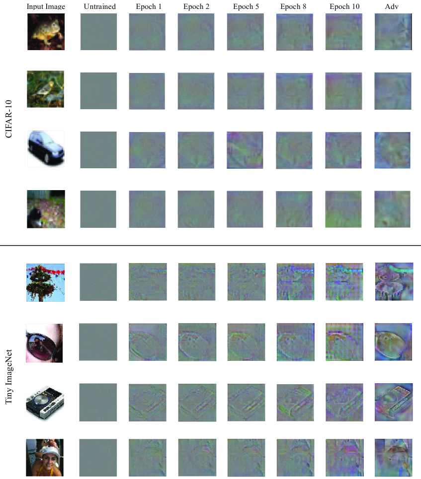
Figure 9: Here we show supplementary examples similar to those in Fig. 4 in the main text. The top four images are the results on CIFAR-10, while the bottom four images are those on Tiny ImageNet. The first column shows the input image $\bm{x}$ in each example. The other columns show the images generated by adversarial transformations with the $f_{b}$ models that are untrained, trained with an increasing number of epochs, and adversarially trained, as labeled on the top line. Each of those images is a visualization of the normalized difference $\bm{x}-\operatorname*{{\mathbb{E}}}_{\tilde{g}\sim\mathcal{T}}\tilde{g}(\bm{x})$, where the expectation is estimated using 5000 samples. It is evident that as the number of training epochs increases, the expectation over transformation $\operatorname*{{\mathbb{E}}}_{\tilde{g}\sim\mathcal{T}}\tilde{g}(\bm{x})$ drifts further away from $\bm{x}$, and the adversarially trained $f_{b}$ model produces an even larger difference.

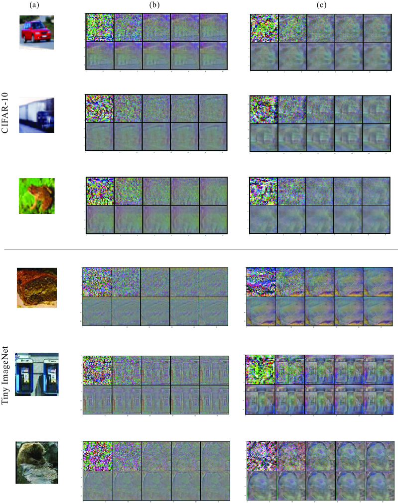
Figure 10: Here we visualize the normalized difference between an input image (shown in column (a)) and its expectation over transformation image $\operatorname*{{\mathbb{E}}}_{\tilde{g}\sim\mathcal{T}}\tilde{g}(\bm{x})$ in our defence model. The top three examples are from CIFAR-10, and the bottom three are from Tiny ImageNet. Column (b) shows the results using $f_{b}$ models with standard training, while column (c) are results with adversarial training. The Expectation over transformation in each example is estimated using an increasing number of samples. The ten sub-images (from left to right, top to bottom) in each group of column (b) and (c) are results in which the expectations over transformation are estimated using 1, 10, 50, 100, 200, 500, 1000, 2000, 5000, 10000 samples of $\tilde{g}(\cdot)$, respectively.

References

- [1] Moustafa Alzantot, Yash Sharma, Supriyo Chakraborty, Huan Zhang, Cho-Jui Hsieh, and Mani B Srivastava. Genattack: Practical black-box attacks with gradient-free optimization. In Proceedings of the Genetic and Evolutionary Computation Conference, pages 1111–1119. ACM, 2019.
- [2] Anish Athalye, Nicholas Carlini, and David A. Wagner. Obfuscated gradients give a false sense of security: Circumventing defenses to adversarial examples. In ICML, pages 274–283, 2018.
- [3] Anish Athalye, Logan Engstrom, Andrew Ilyas, and Kevin Kwok. Synthesizing robust adversarial examples. In International Conference on Machine Learning, pages 284–293, 2018.
- [4] Shumeet Baluja and Ian Fischer. Learning to attack: Adversarial transformation networks. In Proceedings of AAAI-2018, 2018.
- [5] Battista Biggio, Igino Corona, Davide Maiorca, Blaine Nelson, Nedim Šrndić, Pavel Laskov, Giorgio Giacinto, and Fabio Roli. Evasion attacks against machine learning at test time. In Joint European conference on machine learning and knowledge discovery in databases, pages 387–402. Springer, 2013.
- [6] Wieland Brendel, Jonas Rauber, and Matthias Bethge. Decision-based adversarial attacks: Reliable attacks against black-box machine learning models. In International Conference on Learning Representations, 2018.
- [7] Jacob Buckman, Aurko Roy, Colin Raffel, and Ian Goodfellow. Thermometer encoding: One hot way to resist adversarial examples. In International Conference on Learning Representations, 2018.
- [8] Nicholas Carlini and David Wagner. Towards evaluating the robustness of neural networks. In 2017 IEEE Symposium on Security and Privacy (SP), pages 39–57. IEEE, 2017.
- [9] Jianbo Chen and Michael I Jordan. Boundary attack++: Query-efficient decision-based adversarial attack. arXiv preprint arXiv:1904.02144, 2019.
- [10] Guneet S. Dhillon, Kamyar Azizzadenesheli, Jeremy D. Bernstein, Jean Kossaifi, Aran Khanna, Zachary C. Lipton, and Animashree Anandkumar. Stochastic activation pruning for robust adversarial defense. In International Conference on Learning Representations, 2018.
- [11] Yinpeng Dong, Fangzhou Liao, Tianyu Pang, Hang Su, Jun Zhu, Xiaolin Hu, and Jianguo Li. Boosting adversarial attacks with momentum. In Proceedings of the IEEE conference on computer vision and pattern recognition, pages 9185–9193, 2018.
- [12] Alhussein Fawzi, Hamza Fawzi, and Omar Fawzi. Adversarial vulnerability for any classifier. In Advances in Neural Information Processing Systems, pages 1178–1187, 2018.
- [13] Ian Goodfellow, Jonathon Shlens, and Christian Szegedy. Explaining and harnessing adversarial examples. In International Conference on Learning Representations, 2015.
- [14] Chuan Guo, Mayank Rana, Moustapha Cisse, and Laurens van der Maaten. Countering adversarial images using input transformations. In International Conference on Learning Representations, 2018.
- [15] Kaiming He, Xiangyu Zhang, Shaoqing Ren, and Jian Sun. Deep residual learning for image recognition. In Proceedings of the IEEE conference on computer vision and pattern recognition, pages 770–778, 2016.
- [16] Nathan Inkawhich, Wei Wen, Hai (Helen) Li, and Yiran Chen. Feature space perturbations yield more transferable adversarial examples. In The IEEE Conference on Computer Vision and Pattern Recognition (CVPR), June 2019.
- [17] Xiaojun Jia, Xingxing Wei, Xiaochun Cao, and Hassan Foroosh. Comdefend: An efficient image compression model to defend adversarial examples. In The IEEE Conference on Computer Vision and Pattern Recognition (CVPR), June 2019.
- [18] Alex Krizhevsky, Geoffrey Hinton, et al. Learning multiple layers of features from tiny images. Technical report, Citeseer, 2009.
- [19] Alexey Kurakin, Ian J. Goodfellow, and Samy Bengio. Adversarial machine learning at scale. In International Conference on Learning Representations, 2017.
- [20] Yandong Li, Lijun Li, Liqiang Wang, Tong Zhang, and Boqing Gong. Nattack: Learning the distributions of adversarial examples for an improved black-box attack on deep neural networks. In International Conference on Machine Learning, pages 3866–3876, 2019.
- [21] Fangzhou Liao, Ming Liang, Yinpeng Dong, Tianyu Pang, Xiaolin Hu, and Jun Zhu. Defense against adversarial attacks using high-level representation guided denoiser. In Proceedings of the IEEE Conference on Computer Vision and Pattern Recognition, pages 1778–1787, 2018.
- [22] Xuanqing Liu, Minhao Cheng, Huan Zhang, and Cho-Jui Hsieh. Towards robust neural networks via random self-ensemble. In Proceedings of the European Conference on Computer Vision (ECCV), pages 369–385, 2018.
- [23] Zihao Liu, Qi Liu, Tao Liu, Nuo Xu, Xue Lin, Yanzhi Wang, and Wujie Wen. Feature distillation: Dnn-oriented jpeg compression against adversarial examples. In The IEEE Conference on Computer Vision and Pattern Recognition (CVPR), June 2019.
- [24] Jonathan Long, Evan Shelhamer, and Trevor Darrell. Fully convolutional networks for semantic segmentation. In Proceedings of the IEEE conference on computer vision and pattern recognition, pages 3431–3440, 2015.
- [25] Xingjun Ma, Bo Li, Yisen Wang, Sarah M. Erfani, Sudanthi Wijewickrema, Grant Schoenebeck, Michael E. Houle, Dawn Song, and James Bailey. Characterizing adversarial subspaces using local intrinsic dimensionality. In International Conference on Learning Representations, 2018.
- [26] Aleksander Madry, Aleksandar Makelov, Ludwig Schmidt, Dimitris Tsipras, and Adrian Vladu. Towards deep learning models resistant to adversarial attacks. In International Conference on Learning Representations, 2018.
- [27] Chengzhi Mao, Ziyuan Zhong, Junfeng Yang, Carl Vondrick, and Baishakhi Ray. Metric learning for adversarial robustness. arXiv preprint arXiv:1909.00900, 2019.
- [28] Seyed-Mohsen Moosavi-Dezfooli, Alhussein Fawzi, and Pascal Frossard. Deepfool: a simple and accurate method to fool deep neural networks. In Proceedings of the IEEE conference on computer vision and pattern recognition, pages 2574–2582, 2016.
- [29] Aamir Mustafa, Salman Khan, Munawar Hayat, Roland Goecke, Jianbing Shen, and Ling Shao. Adversarial defense by restricting the hidden space of deep neural networks. In The IEEE International Conference on Computer Vision (ICCV), October 2019.
- [30] Nicolas Papernot, Patrick McDaniel, Ian Goodfellow, Somesh Jha, Z. Berkay Celik, and Ananthram Swami. Practical black-box attacks against machine learning. In Proceedings of the 2017 ACM on Asia Conference on Computer and Communications Security, ASIA CCS ’17, pages 506–519, New York, NY, USA, 2017. ACM.
- [31] Edward Raff, Jared Sylvester, Steven Forsyth, and Mark McLean. Barrage of random transforms for adversarially robust defense. In The IEEE Conference on Computer Vision and Pattern Recognition (CVPR), June 2019.
- [32] Jonas Rauber, Wieland Brendel, and Matthias Bethge. Foolbox: A python toolbox to benchmark the robustness of machine learning models. arXiv preprint arXiv:1707.04131, 2017.
- [33] Pouya Samangouei, Maya Kabkab, and Rama Chellappa. Defense-GAN: Protecting classifiers against adversarial attacks using generative models. In International Conference on Learning Representations, 2018.
- [34] Ali Shafahi, W Ronny Huang, Christoph Studer, Soheil Feizi, and Tom Goldstein. Are adversarial examples inevitable? arXiv preprint arXiv:1809.02104, 2018.
- [35] Ali Shafahi, Mahyar Najibi, Amin Ghiasi, Zheng Xu, John Dickerson, Christoph Studer, Larry S Davis, Gavin Taylor, and Tom Goldstein. Adversarial training for free! arXiv preprint arXiv:1904.12843, 2019.
- [36] Mahmood Sharif, Sruti Bhagavatula, Lujo Bauer, and Michael K Reiter. Accessorize to a crime: Real and stealthy attacks on state-of-the-art face recognition. In Proceedings of the 2016 ACM SIGSAC Conference on Computer and Communications Security, pages 1528–1540. ACM, 2016.
- [37] Yucheng Shi, Siyu Wang, and Yahong Han. Curls & whey: Boosting black-box adversarial attacks. In The IEEE Conference on Computer Vision and Pattern Recognition (CVPR), June 2019.
- [38] Aman Sinha, Hongseok Namkoong, and John Duchi. Certifiable distributional robustness with principled adversarial training. In International Conference on Learning Representations, 2018.
- [39] Yang Song, Taesup Kim, Sebastian Nowozin, Stefano Ermon, and Nate Kushman. Pixeldefend: Leveraging generative models to understand and defend against adversarial examples. In International Conference on Learning Representations, 2018.
- [40] Dong Su, Huan Zhang, Hongge Chen, Jinfeng Yi, Pin-Yu Chen, and Yupeng Gao. Is robustness the cost of accuracy? – a comprehensive study on the robustness of 18 deep image classification models. In The European Conference on Computer Vision (ECCV), September 2018.
- [41] Christian Szegedy, Wojciech Zaremba, Ilya Sutskever, Joan Bruna, Dumitru Erhan, Ian Goodfellow, and Rob Fergus. Intriguing properties of neural networks. arXiv preprint arXiv:1312.6199, 2013.
- [42] Olga Taran, Shideh Rezaeifar, Taras Holotyak, and Slava Voloshynovskiy. Defending against adversarial attacks by randomized diversification. In The IEEE Conference on Computer Vision and Pattern Recognition (CVPR), June 2019.
- [43] Simen Thys, Wiebe Van Ranst, and Toon Goedemé. Fooling automated surveillance cameras: adversarial patches to attack person detection. In Proceedings of the IEEE Conference on Computer Vision and Pattern Recognition Workshops, pages 0–0, 2019.
- [44] Florian Tramèr, Alexey Kurakin, Nicolas Papernot, Ian Goodfellow, Dan Boneh, and Patrick McDaniel. Ensemble adversarial training: Attacks and defenses. In International Conference on Learning Representations, 2018.
- [45] Dimitris Tsipras, Shibani Santurkar, Logan Engstrom, Alexander Turner, and Aleksander Madry. Robustness may be at odds with accuracy. arXiv preprint arXiv:1805.12152, 2018.
- [46] Jianyu Wang and Haichao Zhang. Bilateral adversarial training: Towards fast training of more robust models against adversarial attacks. In Proceedings of the IEEE International Conference on Computer Vision, pages 6629–6638, 2019.
- [47] Robert Edwin Wengert. A simple automatic derivative evaluation program. Communications of the ACM, 7(8):463–464, 1964.
- [48] Chaowei Xiao, Bo Li, Jun-Yan Zhu, Warren He, Mingyan Liu, and Dawn Song. Generating adversarial examples with adversarial networks. In Proceedings of the 27th International Joint Conference on Artificial Intelligence, pages 3905–3911. AAAI Press, 2018.
- [49] Chang Xiao, Peilin Zhong, and Changxi Zheng. Resisting adversarial attacks by -winners-take-all. arXiv preprint arXiv:1905.10510, 2019.
- [50] Cihang Xie, Jianyu Wang, Zhishuai Zhang, Zhou Ren, and Alan Yuille. Mitigating adversarial effects through randomization. In International Conference on Learning Representations, 2018.
- [51] Cihang Xie, Yuxin Wu, Laurens van der Maaten, Alan L Yuille, and Kaiming He. Feature denoising for improving adversarial robustness. In Proceedings of the IEEE Conference on Computer Vision and Pattern Recognition, pages 501–509, 2019.
- [52] Cihang Xie, Zhishuai Zhang, Yuyin Zhou, Song Bai, Jianyu Wang, Zhou Ren, and Alan L. Yuille. Improving transferability of adversarial examples with input diversity. In The IEEE Conference on Computer Vision and Pattern Recognition (CVPR), June 2019.
- [53] Dinghuai Zhang, Tianyuan Zhang, Yiping Lu, Zhanxing Zhu, and Bin Dong. You only propagate once: Painless adversarial training using maximal principle. arXiv preprint arXiv:1905.00877, 2019.
- [54] Hongyang Zhang, Yaodong Yu, Jiantao Jiao, Eric Xing, Laurent El Ghaoui, and Michael Jordan. Theoretically principled trade-off between robustness and accuracy. In International Conference on Machine Learning, pages 7472–7482, 2019.