This paper has been accepted for publication at the IEEE Conference on Computer Vision and Pattern Recognition, 2020.
Please cite the paper as: Heng Yang and Luca Carlone,
“In Perfect Shape: Certifiably Optimal 3D Shape Reconstruction from 2D Landmarks”,
In IEEE Conf. on Computer Vision and Pattern Recognition (CVPR), 2020.
In Perfect Shape: Certifiably Optimal
3D Shape Reconstruction from 2D Landmarks

Abstract

We study the problem of 3D shape reconstruction from 2D landmarks extracted in a single image. We adopt the 3D deformable shape model and formulate the reconstruction as a joint optimization of the camera pose and the linear shape parameters. Our first contribution is to apply Lasserre’s hierarchy of convex Sums-of-Squares (SOS) relaxations to solve the shape reconstruction problem and show that the SOS relaxation of minimum order 2 empirically solves the original non-convex problem exactly. Our second contribution is to exploit the structure of the polynomial in the objective function and find a reduced set of basis monomials for the SOS relaxation that significantly decreases the size of the resulting semidefinite program (SDP) without compromising its accuracy. These two contributions, to the best of our knowledge, lead to the first certifiably optimal solver for 3D shape reconstruction, that we name Shape^⋆. Our third contribution is to add an outlier rejection layer to Shape^⋆ using a truncated least squares (TLS) robust cost function and leveraging graduated non-convexity to solve TLS without initialization. The result is a robust reconstruction algorithm, named Shape${\#}$, that tolerates a large amount of outlier measurements. We evaluate the performance of Shape^⋆ and Shape${\#}$ in both simulated and real experiments, showing that Shape^⋆ outperforms local optimization and previous convex relaxation techniques, while Shape${\#}$ achieves state-of-the-art performance and is robust against $70\%$ outliers in the FG3DCar dataset.

1 Introduction

3D object detection and pose estimation from a single image is a fundamental problem in computer vision. Despite the progress in semantic segmentation [12], depth estimation [21], and pose estimation [17, 44], reconstructing the 3D shape and pose of an object from a single image remains a challenging task [2, 50, 38, 43, 19, 36].

A typical approach for 3D shape reconstruction is to first detect 2D landmarks in a single image, and then solve a model-based optimization to lift the 2D landmarks to form a 3D model [49, 50, 36, 26, 41]. For the optimization to be well-posed, the unknown shape is assumed to be a 3D deformable model, composed by a linear combination of basis shapes, handcrafted or learned from a large corpus of training data [9]. The optimization then seeks to jointly optimize the coefficients of the linear combination (shape parameters) and the camera pose to minimize the reprojection errors between the 3D model and the 2D landmarks. This model-based paradigm has been successful in several applications such as face recognition [5, 11], car model fitting [26, 13], and human pose estimation [50, 36].

Despite its long history and broad range of applications, there is still no globally optimal solver for the non-convex optimization problem arising in 3D shape reconstruction. Therefore, most existing solutions adopt a local optimization strategy, which alternates between solving for the camera pose and the shape parameters. These techniques, as shown in prior works [36, 13], require an initial guess for the solution and often get stuck in local minima. In addition, 2D landmark detectors are prone to produce outliers, causing existing methods to be brittle [41]. Therefore, the motivation for this paper is two-fold: (i) to develop a certifiably optimal shape reconstruction solver, and (ii) to develop a robust reconstruction algorithm that is insensitive to a large amount of outlier 2D measurements (e.g., $70\%$).

Contributions. Our first contribution is to formulate the shape reconstruction problem as a polynomial optimization problem and apply Lasserre’s hierarchy of Sums-of-Squares (SOS) relaxations to relax the non-convex polynomial optimization into a convex semidefinite program (SDP). We show the SOS relaxation of minimum order 2 empirically solves the non-convex shape reconstruction problem exactly and provides a global optimality certificate. The second contribution is to apply basis reduction, a technique that exploits the sparse structure of the polynomial in the objective function, to reduce the size of the resulting SDP. We show that basis reduction significantly improves the efficiency of the SOS relaxation without compromising global optimality. To the best of our knowledge, this is the first certifiably optimal solver for shape reconstruction, and we name it Shape^⋆. Our third contribution is to robustify Shape^⋆ by adopting a truncated least squares (TLS) robust cost function and solving the resulting robust estimation problem using graduated non-convexity [4]. The resulting algorithm, named Shape${\#}$, is robust against $70\%$ outliers and does not require an initial guess.

The rest of this paper is organized as follows. Section 2 reviews related work. Section 3 introduces notation and preliminaries on SOS relaxations. Section 4 introduces the shape reconstruction problem. Section 5 develops our SOS solver (Shape^⋆). Section 6 presents an algorithm (Shape${\#}$) to robustify the SOS relaxation against outliers. Section 7 provides experimental results in both simulations and real datasets, while Section 8 concludes the paper.

2 Related Work

We limit our review to optimization-based approaches for 3D shape reconstruction from 2D landmarks. The interested reader can find a review of end-to-end shape and pose reconstruction using deep learning in [19, 38, 18].

Local Optimization. Most existing methods resort to local optimization to solve the non-convex joint optimization of shape parameters and camera pose. Blanz and Vetter [5] propose a method for face recognition by fitting a morphable model of the 3D face shape and texture to a single image using stochastic Newton’s method to escape local minima. Gu and Kanade [11] align a deformable point-based 3D face model by alternatively deforming the 3D model and updating the 3D pose. Using similar alternating optimization, Ramakrishna et al. [36] tackle 3D human pose estimation by finding a sparse set of basis shapes from an over-complete human shape dictionary using projected matching pursuit; the approach is further improved by Fan et al. [10] to include pose locality constraints. Lin et al. [26] demonstrate joint 3D car model fitting and fine-grained classification; car model fitting in cluttered images is investigated in [13]. To mitigate the impact of outlying 2D landmarks, Li et al. [25] propose a RANSAC-type method for car model fitting and Wang et al. [41] replace the least squares estimation with an $\ell_{1}$-norm minimization.

Convex Relaxation. More recently, Zhou et al. [49] develop a convex relaxation, where they first over-parametrize the 3D deformable shape model by associating one rotation with each basis and then relax the resulting Stiefel manifold constraint to its convex envelope. Although showing superior performance compared to local optimization, the convex relaxation in [49] comes with no optimality guarantee and is typically loose in practice. In addition, Zhou et al. [50] model outliers using a sparse matrix and augment the optimization with an $\ell_{1}$ regularization to achieve robustness against $40\%$ outliers. In contrast, we will show that our convex relaxation comes with certifiable optimality, and our robust reconstruction approach can handle $70\%$ outliers.

3 Notation and Preliminaries

We use ${\cal S}^{n}$ to denote the set of $n\times n$ symmetric matrices. We write ${\bm{A}}\in{\cal S}^{n}_{+}$ (resp. ${\bm{A}}\in{\cal S}^{n}_{++}$) to denote that the matrix ${\bm{A}}\in{\cal S}^{n}$ is positive semidefinite (PSD) (resp. positive definite (PD)). Given $\bm{x}=[x_{1},\dots,x_{n}]^{\mathsf{T}}$, we let ${{\mathbb{R}}}[\bm{x}]$ (resp. ${{\mathbb{R}}}[\bm{x}]_{d}$) be the ring of polynomials in $n$ variables with real coefficients (resp. with degree at most $d$), and $[\bm{x}]_{d}$ be the vector of all $\left(\begin{subarray}{c}n+d\\ d\end{subarray}\right)$ monomials with degree up to $d$.

We now give a brief summary of SOS relaxations for polynomial optimization. Our review is based on [6, 31, 23]. We first introduce the notion of SOS polynomial.

Definition 1 (SOS Polynomial [6]).

A polynomial $p(\bm{x})\!\!\in\!\!{{\mathbb{R}}}[\bm{x}]_{2d}$ is said to be a sums-of-squares (SOS) polynomial if there exist polynomials $q_{1},\ldots,q_{m}\!\!\in\!\!{{\mathbb{R}}}[\bm{x}]_{d}$ such that:

$$p(\bm{x})=\sum_{i=1}^{m}q_{i}^{2}(\bm{x}).$$ (1)

We use $\Sigma_{n}$ (resp. $\Sigma_{n,2d})$ to denote the set of SOS polynomials in $n$ variables (resp. with degree at most $2d$). A polynomial $p(\bm{x})\in{{\mathbb{R}}}[\bm{x}]_{2d}$ is SOS if and only if there exists a PSD matrix ${\bm{Q}}\in{\cal S}^{N_{Q}}_{+}$ with $N_{Q}=\left(\begin{subarray}{c}n+d\\ d\end{subarray}\right)$, such that:

$$p(\bm{x})=[\bm{x}]_{d}^{\mathsf{T}}{\bm{Q}}[\bm{x}]_{d},$$ (2)

and ${\bm{Q}}$ is called the Gram matrix of $p(\bm{x})$.

Now consider the following polynomial optimization:

$$\min_{\bm{x}\in{{\mathbb{R}}^{n}}} f(\bm{x})$$ (3)

$$s.t. h_{i}(\bm{x})=0,i=1,\dots,m,$$

$$g_{k}(\bm{x})\geq 0,k=1,\dots,l,$$

where $f,h_{i},g_{k}\in{{\mathbb{R}}}[\bm{x}]$ are all polynomials and let ${\cal X}$ be the feasible set defined by $h_{i},g_{k}$. For convenience, denote $\bm{h}:=(h_{1},\dots,h_{m})$, $g_{0}:=1$ and $\bm{g}=(g_{0},\dots,g_{l})$. We call

$$\langle\bm{h}\rangle:=\{h\in{{\mathbb{R}}}[\bm{x}]:h=\sum_{i=1}^{m}\lambda_{i}h_{i},\lambda_{i}\in{{\mathbb{R}}}[\bm{x}]\},$$ (4)

$$\langle\bm{h}\rangle_{2\beta}:=\{h\in\langle\bm{h}\rangle:\text{deg}(\lambda_{i}h_{i})\leq 2\beta\},$$ (5)

the ideal and the $2\beta$-th truncated ideal of $\bm{h}$, where $\text{deg}(\cdot)$ is the degree of a polynomial. The ideal is simply a summation of polynomials with polynomial coefficients, a construct that will simplify the notation later on. We call

$$Q(\bm{g}):=\{g\in{{\mathbb{R}}}[\bm{x}]:g=\sum_{k=0}^{m}s_{k}g_{k},s_{k}\in\Sigma_{n}\},$$ (6)

$$Q_{\beta}(\bm{g}):=\{g\in Q(\bm{g}):\text{deg}(s_{k}g_{k})\leq 2\beta\},$$ (7)

the quadratic module and the $\beta$-th truncated quadratic module generated from $\bm{g}$. Note that the quadratic module is similar to the ideal, except now we require the polynomial coefficients to be SOS. Apparently, if $p(\bm{x})\in\langle\bm{h}\rangle+Q(\bm{g})$, then $p(\bm{x})$ is nonnegative on ${\cal X}$. Putinar’s Positivstellensatz [35] describes when the reverse is also true.

Theorem 2 (Putinar’s Positivstellensatz [35]).

Let ${\cal X}$ be the feasible set of problem (3). Assume $\langle\bm{h}\rangle+Q(\bm{g})$ is Archimedean, i.e., $M-\|\bm{x}\|_{2}^{2}\in\langle\bm{h}\rangle_{2\beta}+Q_{\beta}(\bm{g})$ for some $\beta\in\mathbb{N}$ and $M>0$. If $p(\bm{x})\in{{\mathbb{R}}}[\bm{x}]$ is positive on ${\cal X}$, then $p(\bm{x})\in\langle\bm{h}\rangle+Q(\bm{g})$.

Based on Putinar’s Positivstellensatz, Lasserre [22] derived a sequence of SOS relaxations that approximates the global minimum of problem (3) with increasing accuracy. The key insight behind Lasserre’s hierarchy is twofold. The first insight is that problem (3), which we can write succinctly as $\min_{\bm{x}\in{\cal X}}f(x)$, can be equivalently written as $\displaystyle\max_{\bm{x},\gamma}\gamma,s.t.f(x)-\gamma\geq 0\text{ on }{\cal X}$ (intuition: the latter pushes the lower bound $\gamma$ to reach the global minimum of $f(\bm{x})$). The second intuition is that we can rewrite the condition $f(x)-\gamma\geq 0\text{ on }{\cal X}$, using Putinar’s Positivstellensatz (Theorem 2), leading to the following hierarchy of Sums-of-Squares relaxations.

Theorem 3 (Lasserre’s Hierarchy [22]).

Lasserre’s hierarchy of order $\beta$ is the following SOS program:

$$\max\quad\gamma,\quad s.t.\;\;f(\bm{x})-\gamma\in\langle\bm{h}\rangle_{2\beta}+Q_{\beta}(\bm{g}),$$ (8)

which can be written as a standard SDP. Moreover, let $f^{\star}$ be the global minimum of (3) and $f^{\star}_{\beta}$ be the optimal value of (8), then $f^{\star}_{\beta}$ monotonically increases and $f^{\star}_{\beta}\rightarrow f^{\star}$ when $\beta\rightarrow\infty$. More recently, Nie [31] proved that under Archimedeanness, Lasserre’s hierarchy has finite convergence generically (i.e., $f^{\star}_{\beta}=f^{\star}$ for some finite $\beta$).

In computer vision, Lasserre’s hierarchy was first used by Kahl and Henrion [16] to minimize rational functions arising in geometric reconstruction problems, and more recently by Probst et al. [34] as a framework to solve a set of 3D vision problems. In this paper we will show that the SOS relaxation as written in eq. (8) allows using basis reduction to exploit the sparsity pattern of polynomials and leads to significantly smaller semidefinite programs.

4 Problem Statement: Shape Reconstruction

Assume we are given $N$ pixel measurements ${\bm{Z}}=[\bm{z}_{1},\dots,\bm{z}_{N}]\in{{\mathbb{R}}^{2\times N}}$ (the 2D landmarks), generated from the projection of points belonging to an unknown 3D shape ${\bm{S}}\in{{\mathbb{R}}^{3\times N}}$ onto an image. Further assume the shape ${\bm{S}}$ that can be represented as a linear combination of $K$ predefined basis shapes ${\bm{B}}_{k}\in{{\mathbb{R}}^{3\times N}}$, i.e. ${\bm{S}}=\sum_{k=1}^{K}c_{k}{\bm{B}}_{k}$, where $\{c_{k}\}_{k=1}^{K}$ are (unknown) shape coefficients. Then, the generative model of the 2D landmarks reads:

$$\bm{z}_{i}=\Pi{\bm{R}}\left(\sum_{k=1}^{K}c_{k}{\bm{B}}_{ki}\right)+\bm{t}+\bm{\epsilon}_{i},i=1,\dots,N,$$ (9)

where ${\bm{B}}_{ki}$ denotes the $i$-th 3D point on the $k$-th basis shape, $\bm{\epsilon}_{i}\in{{\mathbb{R}}^{2}}$ models the measurement noise, and $\Pi$ is the (known) weak perspective projection matrix:

$$\Pi=\left[\begin{array}[]{ccc}s_{x}&0&0\\ 0&s_{y}&0\end{array}\right],$$ (12)

with $s_{x}$ and $s_{y}$ being constants. In eq. (9), ${\bm{R}}\in\mathrm{SO}(3)$ and $\bm{t}\in{{\mathbb{R}}^{2}}$ model the (unknown) rotation and translation of the shape ${\bm{S}}$ relative to the camera (only a 2D translation can be estimated). The shape reconstruction problem consists in the joint estimation of the shape parameters $\{c_{k}\}_{k=1}^{K}$ and the camera pose $({\bm{R}},\bm{t})$.

Without loss of generality, we adopt the nonnegative sparse coding (NNSC) convention [50] and assume all the coefficients $c_{k}$ are nonnegative. Due to the existence of noise, we solve the following weighted least squares optimization with Lasso ($\ell_{1}$-norm) regularization:

$$\min_{\begin{subarray}{c}c_{k}\geq 0,k=1,\dots,K\\ \bm{t}\in{{\mathbb{R}}^{2}},{\bm{R}}\in\mathrm{SO}(3)\end{subarray}} \!\!\displaystyle\!\!\sum_{i=1}^{N}w_{i}\!\!\left\|\bm{z}_{i}\!-\!\Pi{\bm{R}}\left(\sum_{k=1}^{K}c_{k}{\bm{B}}_{ki}\right)\!-\!\bm{t}\right\|^{2}\!\!\!\!+\!\alpha\!\!\sum_{k=1}^{K}\left|c_{k}\right|$$ (13)

The $\ell_{1}$-norm regularization (controlled by a given constant $\alpha$) encourages the coefficients $c_{k}$ to be sparse when the shape ${\bm{S}}$ is generated from only a subset of the basis shapes [50] (note that the $\ell_{1}$-norm becomes redundant when using the NNSC convention). Contrary to previous approaches [50, 36], we explicitly associate a given weight $w_{i}\geq 0$ to each 2D measurement $\bm{z}_{i}$ in eq. (13). On the one hand, this allows accommodating heterogeneous noise in the 2D landmarks (e.g., $w_{i}=1/\sigma_{i}^{2}$ when the noise $\bm{\epsilon}_{i}$ is Gaussian, $\bm{\epsilon}_{i}\sim{\cal N}({\mathbf{0}},\sigma_{i}^{2}{\mathbf{I}}_{2})$). On the other hand, as shown in Section 6, the weighted least squares framework is useful to robustify (13) against outliers.

5 Certifiably Optimal Shape Reconstruction

This section shows how to develop a certifiably optimal solver for problem (13). Our first step is to algebraically eliminate the translation $\bm{t}$ and obtain a translation-free shape reconstruction problem, as shown below.

Theorem 4 (Translation-free Shape Reconstruction).

The shape reconstruction problem (13) is equivalent to the following translation-free optimization:

$$\min_{\begin{subarray}{c}c_{k}\geq 0,k=1,\dots,K\\ {\bm{R}}\in\mathrm{SO}(3)\end{subarray}} \!\!\!\displaystyle\sum_{i=1}^{N}\left\|\tilde{\bm{z}}_{i}\!-\!\Pi{\bm{R}}\left(\sum_{k=1}^{K}c_{k}\tilde{{\bm{B}}}_{ki}\right)\right\|^{2}\!\!+\!\alpha\sum_{k=1}^{K}|c_{k}|$$ (14)

where $\tilde{\bm{z}}_{i}$ and $\tilde{{\bm{B}}}_{ki}$ can be computed as follows:

$$\tilde{\bm{z}}_{i}=\sqrt{w_{i}}(\bm{z}_{i}-\bar{\bm{z}}^{w}),\text{ with }\bar{\bm{z}}^{w}=\frac{\sum_{i=1}^{N}w_{i}\bm{z}_{i}}{\sum_{i=1}^{N}w_{i}},$$ (15)

$$\tilde{{\bm{B}}}_{ki}=\sqrt{w_{i}}({\bm{B}}_{ki}-\bar{{\bm{B}}}^{w}_{k}),\text{ with }\bar{{\bm{B}}}^{w}_{k}=\frac{\sum_{i=1}^{N}w_{i}{\bm{B}}_{ki}}{\sum_{i=1}^{N}w_{i}}.$$ (16)

Further, let ${\bm{R}}^{\star}$ and $c_{k}^{\star},k=1,\dots,K,$ be the global minimizer of the above translation-free optimization (14), then the optimal translation $\bm{t}^{\star}$ can be recovered as:

$$\bm{t}^{\star}=\bar{\bm{z}}^{w}-\Pi{\bm{R}}^{\star}\left(\sum_{k=1}^{K}c_{k}^{\star}\bar{{\bm{B}}}^{w}_{k}\right).$$ (17)

A formal proof of Theorem 4 can be found in the Supplementary Material. The intuition behind Theorem 4 is that if we express the landmark coordinates and 3D basis shapes with respect to their (weighted) centroids $\bar{\bm{z}}^{w}$ and $\bar{{\bm{B}}}^{w}_{k},k=1,\dots,K$, we can remove the dependence on the translation $\bm{t}$. This strategy is inspired by Horn’s method for point cloud registration [15], and generalizes [50] to the weighted and non-centered case.

5.1 SOS Relaxation

This section applies Lasserre’s hierarchy as described in Theorem 3 to solve the translation-free shape reconstruction problem (14). We do this in two steps: we first show problem (14) can be formulated as a polynomial optimization in the form (3); and then we add valid constraints to make the feasible set Archimedean.

Polynomial Optimization Formulation. Denote $\bm{c}=[c_{1},\dots,c_{k}]^{\mathsf{T}}\in{{\mathbb{R}}^{K}}$, $\bm{r}=\text{vec}({\bm{R}})=[\bm{r}_{1}^{\mathsf{T}},\bm{r}_{2}^{\mathsf{T}},\bm{r}_{3}^{\mathsf{T}}]^{\mathsf{T}}\in{{\mathbb{R}}^{9}}$, with $\bm{r}_{i},i=1,2,3$ being the $i$-th column of ${\bm{R}}$, then $\bm{x}:=[\bm{c}^{\mathsf{T}},\bm{r}^{\mathsf{T}}]^{\mathsf{T}}\in{{\mathbb{R}}^{K+9}}$ is the unknown decision vector in (3). Consider the first term in the objective function of (14). We can write:

$$\scriptstyle q_{i}(\bm{x}):=\left\|\tilde{\bm{z}}_{i}-\Pi{\bm{R}}\left(\sum_{k=1}^{K}c_{k}\tilde{{\bm{B}}}_{ki}\right)\right\|^{2}=\left\|\tilde{\bm{z}}_{i}-\Pi\sum_{k=1}^{K}c_{k}{\bm{R}}\tilde{{\bm{B}}}_{ki}\right\|^{2},$$ (18)

then it becomes clear that $q_{i}(\bm{x})$ is a polynomial function of $\bm{x}$ with degree 4. Because the Lasso regularization is linear in $\bm{c}$, the objective function $f(\bm{x})$ is a degree-4 polynomial.

Now we consider the feasible set of (14). The inequality constraints $c_{k}\geq 0$ are already in generic form (3) with $g_{k}(\bm{x})=c_{k},k=1,\dots,K$, being degree-1 polynomials. As for the ${\bm{R}}\in\mathrm{SO}(3)$ constraint, it has already been shown in related work [39, 7] that enforcing ${\bm{R}}\in\mathrm{SO}(3)$ is equivalent to imposing 15 quadratic equality constraints.

Lemma 5 (Quadratic Constraints for $\mathrm{SO}(3)$ [39, 7]).

For a matrix ${\bm{R}}\in{{\mathbb{R}}^{3\times 3}}$, the constraint ${\bm{R}}\in\mathrm{SO}(3)$ (where $\mathrm{SO}(3):=\{{\bm{R}}:{\bm{R}}^{\mathsf{T}}{\bm{R}}={\mathbf{I}}_{3},\det{{\bm{R}}}=+1\}$ is the set of proper rotation matrices) is equivalent to the following set of degree-2 polynomial equality constraints ($h_{i}(\bm{x})=0,i=1,\dots,15$):

$$\begin{cases}h_{1}=1-\|\bm{r}_{1}\|^{2},h_{2}=1-\|\bm{r}_{2}\|^{2},h_{3}=1-\|\bm{r}_{3}\|^{2}\\ h_{4}=\bm{r}_{1}^{\mathsf{T}}\bm{r}_{2},\quad h_{5}=\bm{r}_{2}^{\mathsf{T}}\bm{r}_{3},\quad h_{6}=\bm{r}_{3}^{\mathsf{T}}\bm{r}_{1}\\ h_{7,8,9}=\bm{r}_{1}\times\bm{r}_{2}-\bm{r}_{3}\\ h_{10,11,12}=\bm{r}_{2}\times\bm{r}_{3}-\bm{r}_{1}\\ h_{13,14,15}=\bm{r}_{3}\times\bm{r}_{1}-\bm{r}_{2}\end{cases}$$ (19)

where $\bm{r}_{i}\in{{\mathbb{R}}^{3}},i=1,2,3$, denotes the $i$-th column of ${\bm{R}}$ and “$\times$” represents the vector cross product.

In eq. (19), $h_{1,2,3}$ constrain the columns to be unit vectors, $h_{4,5,6}$ constrain the columns to be mutually orthogonal, and $h_{7-15}$ constrain the columns to satisfy the right-hand rule (i.e., the determinant constraint).

In summary, the translation-free problem (14) is equivalent to a polynomial optimization with a degree-4 objective $f(\bm{x})$, constrained by 15 quadratic equalities $h_{i}(\bm{x})$ (eq. (19)) and $K$ linear inequalities $g_{k}(\bm{x})=c_{k}$.

Archimedean Feasible Set. The issue with the feasible set defined by inequalities $c_{k}\geq 0$ and equalities (19) is that $\langle\bm{h}\rangle+Q(\bm{g})$ is not Archimedean, which can be easily seen from the unboundedness of the linear inequality $c_{k}\geq 0$. However, we know the linear coefficients must be bounded because the pixel measurement values ${\bm{Z}}$ lie in a bounded set (the 2D image). Therefore, we propose to normalize the 2D measurements and the 3D basis shapes: (i) for 2D measurements ${\bm{Z}}$, we first divide them by $s_{x}$ and $s_{y}$ (eq. (12)), and then scale them such that they lie inside a unit circle; (ii) for each 3D basis shape ${\bm{B}}_{k}$, we scale ${\bm{B}}_{k}$ such that it lies inside a unit sphere. With this proper normalization, we can add the following degree-2 inequality constraints ($c_{k}^{2}\leq 1$) that bound the linear coefficients:

$$g_{K+k}(\bm{x})=1-c_{k}^{2},k=1,\dots,K.$$ (20)

Now we can certify the Archimedeanness of $\langle\bm{h}\rangle+Q(\bm{g})$:

$$K+3-\|\bm{x}\|_{2}^{2}=\underbrace{\sum_{k=1}^{K}1\cdot g_{K+k}}_{\in Q_{1}(\bm{g})}+\underbrace{h_{1}+h_{2}+h_{3}}_{\in\langle\bm{h}\rangle_{2}},$$ (21)

with $M=K+3$ and $\beta=1$ (cf. Theorem 2).

Apply Lasserre’s Hierarchy. With Archimedeanness, we can now apply Lasserre’s hierarchy of SOS relaxations.

Proposition 6 (SOS Relaxations for Shape Reconstruction).

The SOS relaxation of order $\beta$ ($\beta\geq 2$) for the translation-free shape reconstruction problem (14) is the following convex semidefinite program:

$$\max_{\begin{subarray}{c}\gamma\in{{\mathbb{R}}},{\bm{S}}_{0}\in{\cal S}^{N_{0}}_{+}\\ {\bm{S}}_{k}\in{\cal S}_{+}^{N_{s}},\;k=1,\dots,2K\\ \bm{\lambda}_{i}\in{{\mathbb{R}}^{N_{\lambda}}},i=1,\dots,15\end{subarray}} \gamma$$ (22)

$$s.t. f(\bm{x})-\gamma=[\bm{x}]_{\beta}^{\mathsf{T}}{\bm{S}}_{0}[\bm{x}]_{\beta}+$$ (23)

$$\sum_{k=1}^{2K}\left([\bm{x}]_{\beta-1}^{\mathsf{T}}{\bm{S}}_{k}[\bm{x}]_{\beta-1}\right)g_{k}(\bm{x})+$$

$$\sum_{i=1}^{15}\left(\bm{\lambda}_{i}^{\mathsf{T}}[\bm{x}]_{2\beta-2}\right)h_{i}(\bm{x}),$$

where $f(\bm{x})$ is the objective function defined in (14), $g_{k}(\bm{x}),k=1,\dots,2K$ are the inequality constraints $c_{k},1-c_{k}^{2}$, $h_{i}(\bm{x}),i=1,\dots,15$ are the equality constraints defined in (19), and $N_{0}:=\left(\begin{subarray}{c}K+9+\beta\\ \beta\end{subarray}\right)$, $N_{s}:=\left(\begin{subarray}{c}K+8+\beta\\ \beta-1\end{subarray}\right)$, $N_{\lambda}:=\left(\begin{subarray}{c}K+7+2\beta\\ 2\beta-2\end{subarray}\right)$ are the sizes of matrices and vectors.

While a formal proof of Proposition 6 is given in the Supplementary Material, we observe that (22) immediately results from the application of Lasserre’s hierarchy to (8), by parametrizing $Q_{\beta}(\bm{g})$ with monomial bases $[\bm{x}]_{\beta-1}$, $[\bm{x}]_{\beta}$ and PSD matrices ${\bm{S}}_{0}$, ${\bm{S}}_{k},k=1,\dots,2K$ (one for each $g_{k}$), and by parametrizing $\langle\bm{h}\rangle_{2\beta}$ with monomial basis $[\bm{x}]_{2\beta-2}$ and coefficient vectors $\bm{\lambda}_{i},i=1,\dots,15$ (one for each $h_{i}$). Problem (22) can be written as an SDP and solved globally using standard convex solvers (e.g. YALMIP [27]). We call the SDP written in (22) the primal SDP. The dual SDP of (22) can be derived using moment relaxation [22, 24, 23], which is readily available in GloptiPoly 3 [14].

Extract Solutions from SDP. After solving the SDP (22), we can extract solutions to the original non-convex problem (14), a procedure we call rounding.

Proposition 7 (Rounding and Duality Gap).

Let $f^{\star}_{\beta}=\gamma^{\star}$ and ${\bm{S}}_{0}^{\beta\star},{\bm{S}}_{k}^{\beta\star},\bm{\lambda}_{i}^{\beta\star}$ be the optimal solutions to the SDP (22) at order $\beta$; compute $\bm{v}^{\beta\star}$ as the eigenvector corresponding to the minimum eigenvalue of ${\bm{S}}_{0}^{\beta\star}$, and then normalize $\bm{v}^{\beta\star}$ such that the first entry is equal to 1. Then an approximate solution to problem (14) can be obtained as:

$$\hat{\bm{c}}^{\beta}=\text{proj}_{\bm{g}}([\bm{v}^{\beta\star}]_{\bm{c}});\quad\hat{\bm{r}}^{\beta}=\text{proj}_{\bm{h}}([\bm{v}^{\beta\star}]_{\bm{r}}),$$ (24)

where $[\bm{v}^{\beta\star}]_{\bm{c}}$ (resp. $[\bm{v}^{\beta\star}]_{\bm{r}}$) denotes the entries of $\bm{v}^{\beta\star}$ corresponding to monomials $\bm{c}$ (resp. $\bm{r}$), and $\text{proj}_{\bm{g}}$ (resp. $\text{proj}_{\bm{h}}$) denotes projection to the feasible set defined by $\bm{g}$ (resp. $\bm{h}$). Specifically for problem (14), $\text{proj}_{\bm{g}}$ is rounding each coefficient $c_{k}$ to the $[0,1]$ interval, and $\text{proj}_{\bm{h}}$ is the projection to $\mathrm{SO}(3)$. Moreover, let $\hat{f}_{\beta}$ be the value of the objective function evaluated at the approximate solution $\hat{\bm{x}}^{\beta}:=[(\hat{\bm{c}}^{\beta})^{\mathsf{T}},(\hat{\bm{r}}^{\beta})^{\mathsf{T}}]^{\mathsf{T}}$, then the following inequality holds (weak duality):

$$f^{\star}_{\beta}\leq f^{\star}\leq\hat{f}_{\beta},$$ (25)

where $f^{\star}$ is the true (unknown) global minimum of problem (14). We define the relative duality gap $\eta_{\beta}$ as:

$$\eta_{\beta}=(\hat{f}_{\beta}-f^{\star}_{\beta})/\hat{f}_{\beta},$$ (26)

which quantifies the quality of the SOS relaxation.

Certifiable Global Optimality. Besides extracting solutions to the original problem, we can also verify when the SOS relaxation solves the original problem exactly.

Theorem 8 (Certificate of Global Optimality).

Let $f^{\star}_{\beta}=\gamma^{\star}$ and ${\bm{S}}_{0}^{\beta\star}$ be the optimal solutions to the SDP (22) at order $\beta$. If $\text{corank}({\bm{S}}_{0}^{\beta\star})=1$ (the corank is the dimension of the null space of ${\bm{S}}_{0}^{\beta\star}$), then $f^{\star}_{\beta}$ is the global minimum of problem (14), and the relaxation is said to be tight at order $\beta$. Moreover, the relative duality gap $\eta_{\beta}=0$ and the solution $\hat{\bm{x}}^{\beta}$ extracted using Proposition 7 is the unique global minimizer of problem (14).

The proof of Theorem 8 is given in the Supplementary Material. Empirically (Section 7), we observed that the relaxation is always tight at the minimum relaxation order $\beta=2$. Note that even when the relaxation is not tight, one can still obtain an approximate solution using Proposition 7 and quantify how suboptimal the approximate solution is using the relative duality gap $\eta_{\beta}$.

5.2 Basis Reduction

Despite the theoretical soundness and finite convergence at order $\beta=2$, the size of the SDP (22) is $N_{0}=\left(\begin{subarray}{c}K+9+\beta\\ \beta\end{subarray}\right)$, which for $\beta=2$ becomes $\left(\begin{subarray}{c}K+11\\ 2\end{subarray}\right)$, implying that the size of the SDP grows quadratically in the number of bases $K$. Although there have been promising advances in improving the scalability of SDP solvers (see [29] for a thorough review), such as exploiting sparsity [42, 40, 30] and low-rankness [8, 37], in this section we demonstrate a simple yet effective approach, called basis reduction, that exploits the structure of the objective function to significantly reduce the size of the SDP in (22).

In a nutshell, basis reduction methods seek to find a smaller, but still expressive enough, subset of the full vector of monomials $[\bm{x}]_{\beta}$ on the right-hand side (RHS) of eq. (23), to explain the objective function $f(\bm{x})$ on the left-hand side (LHS). There exist standard approximation algorithms for basis reduction, discussed in [32, 33] and implemented in YALMIP [28]. However, in practice we found the basis selection method in YALMIP failed to find any reduction for the SDP (22). Therefore, here we propose a problem-specific reduction, which follows from the examination of which monomials appear on the LHS of (23).

Proposition 9 (SOS Relaxation with Basis Reduction).

The SOS relaxation of order $\beta=2$ with basis reduction for the translation-free shape reconstruction problem (14) is the following convex semidefinite program:

$$\max_{\begin{subarray}{c}\gamma\in{{\mathbb{R}}},{\bm{S}}_{0}\in{\cal S}_{+}^{N_{0}^{\prime}}\\ {\bm{S}}_{k}\in{\cal S}_{+}^{N_{s}^{\prime}},k=1,\dots,2K,\\ \bm{\lambda}_{i}\in{{\mathbb{R}}^{N_{\lambda}^{\prime}}},i=1,\dots,15\end{subarray}} \gamma$$ (27)

$$s.t. f(\bm{x})-\gamma=m_{2}(\bm{x})^{\mathsf{T}}{\bm{S}}_{0}m_{2}(\bm{x})+$$ (28)

$$\sum_{k=1}^{2K}([\bm{r}]_{1}^{\mathsf{T}}{\bm{S}}_{k}[\bm{r}])g_{k}(\bm{x})+$$

$$\sum_{i=1}^{15}(\bm{\lambda}_{i}^{\mathsf{T}}[\bm{c}]_{2})h_{i}(\bm{x}),$$

where $N_{0}^{\prime}=10K+10$, $N_{s}^{\prime}=10$, $N_{\lambda}^{\prime}=\left(\begin{subarray}{c}K+2\\ 2\end{subarray}\right)$, and $m_{2}(\bm{x})=[1,\bm{c}^{\mathsf{T}},\bm{r}^{\mathsf{T}},\bm{c}^{\mathsf{T}}\otimes\bm{r}^{\mathsf{T}}]^{\mathsf{T}}\in{{\mathbb{R}}^{N_{0}}}$, and where $\otimes$ is the Kronecker product.

Comparing the SDP (27) and (22), the most significant change is replacing the full monomial basis $[\bm{x}]_{\beta}$ in (22) with a much smaller monomial basis $m_{2}(\bm{x})$ that excludes degree-2 monomials purely supported in $\bm{c}$ and $\bm{r}$. This reduction is motivated by analyzing the monomial terms in $f(\bm{x})$. Although a formal proof of the equivalence between (22) and (27) remains open, we provide an intuitive explanation in the Supplementary Material. After basis reduction, the size of the SDP (27) is $N_{0}^{\prime}=10K+10$, which is linear in $K$ and much smaller than the size of the original SDP (22) $N_{k}=\left(\begin{subarray}{c}K+11\\ 2\end{subarray}\right)$. Section 7 numerically shows that the SDP after basis reduction gives the same (tight) solution as the original SDP.

5.3 Shape^⋆: Algorithm Summary

To summarize the derivation in this section, our solver for the shape reconstruction problem (13), named Shape^⋆, works as follows. It first solves the SDP (27) and applies the rounding described in Proposition 7 to compute an estimate of the shape parameters $c_{k}$ and rotation ${\bm{R}}$ and possibly certify its optimality. Then, Shape^⋆ uses the closed-form expression (17) to retrieve the translation estimate $\bm{t}$.

6 Robust Outlier Rejection

Section 5 proposed a certifiably optimal solver for problem (13). However, the least squares formulation (13) tends to be sensitive to outliers: the pixel measurements ${\bm{Z}}$ in eq. (9) are typically produced by learning-based or handcrafted detectors [50], which might produce largely incorrect measurements (e.g. due to wrong data association $\bm{z}_{i}\leftrightarrow{\bm{B}}_{ki}$), which in turn leads to poor shape reconstruction results. This section shows how to regain robustness by iteratively solving the weighted least squares problem (13) and adjusting the weights $w_{i}$ to reject outliers.

The key insight is to substitute the least square penalty in (13) with a robust cost function, namely the truncated least squares (TLS) cost [47, 46, 20, 48]. Hence, we propose the following TLS shape reconstruction formulation:

$$\!\!\!\min_{\begin{subarray}{c}c_{k}\geq 0,\\ k=1,\dots,K\\ \bm{t}\in{{\mathbb{R}}^{2}},{\bm{R}}\in\mathrm{SO}(3)\end{subarray}} \displaystyle\sum_{i=1}^{N}\rho_{\bar{c}}\left(r_{i}(c_{k},{\bm{R}},\bm{t})\right)+\alpha\!\sum_{k=1}^{K}\!c_{k}$$ (29)

where $r_{i}(c_{k},{\bm{R}},\bm{t}):=\left\|\bm{z}_{i}\!-\!\Pi{\bm{R}}\left(\sum_{k=1}^{K}c_{k}{\bm{B}}_{ki}\right)\!-\!\bm{t}\right\|$ (introduced for notational convenience), and $\rho_{\bar{c}}(r)=\min(r^{2},\bar{c}^{2})$ implements a truncated least squares cost, which is quadratic for small residuals and saturates to a constant value for residuals larger than a maximum error $\bar{c}$.

Our second insight is that $\rho_{\bar{c}}(r)$ can be written as $\rho_{\bar{c}}(r)=\min_{w\in\{0,1\}}wr^{2}+(1-w)\bar{c}^{2}$, by introducing extra slack binary variables $w\in\{0,1\}$. Therefore, we can write problem (29) equivalently as:

$$\!\!\!\min_{\begin{subarray}{c}c_{k}\geq 0,k=1,\dots,K,\\ w_{i}\in\{0,1\},i=1,\dots,N\\ \bm{t}\in{{\mathbb{R}}^{2}},{\bm{R}}\in\mathrm{SO}(3)\end{subarray}} \displaystyle\sum_{i=1}^{N}w_{i}\left(r_{i}(c_{k},{\bm{R}},\bm{t})\right)\!+\!(1\!-\!w_{i})\bar{c}^{2}\!\!+\!\alpha\!\sum_{k=1}^{K}\!\!c_{k}$$ (30)

The final insight is that now we can minimize (30) by iteratively minimizing (i) over $c_{k},{\bm{R}},\bm{t}$ (with fixed weights $w_{i}$), and (ii) over the weights $w_{i}$ (with fixed $c_{k},{\bm{R}},\bm{t}$). The rationale for this approach is that step (i) can be implemented using Shape^⋆ (since in this case the weights are fixed), and step (ii) can be implemented in closed-form. To improve convergence of this iterative algorithm, we adopt graduated non-convexity [4, 45], which starts with a convex approximation of problem (30) and uses a control parameter $\mu$ to gradually increase the amount of non-convexity, till (for large $\mu$) one solves (30). The resulting algorithm named Shape${\#}$ is given in Algorithm 1. We refer the reader to the Supplementary Material and [45] for a complete derivation of Algorithm 1 and for the closed-form expression of the weight update in line 1 of the algorithm.

input :  measurements $\bm{z}_{i},i=1,\ldots,N$,

basis shapes ${\bm{B}}_{k},k=1,\ldots,M$

maximum error $\bar{c}$, regularization constant $\alpha$

output :  shape reconstruction: $c_{k}^{\star},{\bm{R}}^{\star},\bm{t}^{\star}$

/* Initialization */

1 $w_{i}^{(0)}=1,\quad i=1,\dots,N$

2 $\mu^{(0)}=10^{-4}$

/* Iterations */

3 for  $\tau=1:\text{maxIter}$  do

       /* Variable update */

4       $c_{k}^{(\tau)},{\bm{R}}^{(\tau)},\bm{t}^{(\tau)}=\text{{\sf Shape${}^{\star}$}}(\bm{z}_{i},{\bm{B}}_{k},\alpha,w_{i}^{(\tau-1)},\mu^{(\tau-1)})$

       /* Compute residual errors */

5       $r_{i}^{(\tau)}=\|\bm{z}_{i}-\Pi{\bm{R}}^{(\tau)}\left(\sum_{k=1}^{K}c_{k}^{(\tau)}{\bm{B}}_{ki}\right)-\bm{t}^{(\tau)}\|$

       /* Weight update */

6       $w_{i}^{(\tau)}=\text{weightUpdate}(r_{i}^{(\tau)},\bar{c},\mu^{(\tau-1)})$

       /* Compute objective function */

7       $f^{(\tau)}=\text{computeObjective}(r_{i}^{(\tau)},w_{i}^{(\tau)},\mu^{(\tau-1)},\alpha,\bar{c})$

       /* Check convergence ($\tau>1$) */

8       if  $|f^{(\tau)}-f^{(\tau-1)}|<10^{-10}$  then

9             break

      /* Update control parameter $\mu$ */

10       $\mu^{(\tau)}=2\cdot\mu^{(\tau-1)}$

return $c_{k}^{(\tau)},{\bm{R}}^{(\tau)},\bm{t}^{(\tau)}$.

Algorithm 1 Robust Shape Reconstruction.

Shape${\#}$ is deterministic and does not require an initial guess. We remark that the graduated non-convexity scheme in Shape${\#}$ (contrarily to Shape^⋆) is not guaranteed to converge to an optimal solution of (30), but we show in the next section that it is empirically robust to $70\%$ outliers.

7 Experiments

Implementation details. Both Shape^⋆ and Shape${\#}$ are implemented in Matlab, with both SOS relaxations (22) and (27) implemented using YALMIP [27] and the resulting SDPs solved using MOSEK [1].

7.1 Efficiency Improvement by Basis Reduction

We first evaluate the efficiency improvement due to basis reduction in simulation. We fix the number of correspondences $N=100$, and increase the number of basis shapes $K=5,10,20$. At each $K$, we first randomly generate $K$ basis shapes ${\bm{B}}_{1},\dots,{\bm{B}}_{K}\in{{\mathbb{R}}^{3\times N}}$, with entries sampled independently from a Normal distribution ${\cal N}(0,1)$. Then $K$ linear coefficients $\bm{c}=[c_{1},\dots,c_{K}]^{\mathsf{T}}$ are uniformly sampled from the interval $[0,1]$, and a rotation matrix ${\bm{R}}$ is randomly chosen. The 2D measurements ${\bm{Z}}$ are computed from the generative model (9) with $\bm{t}=\bm{0}$, $s_{x}=s_{y}=1$ for $\Pi$, and additive noise $\bm{\epsilon}_{i}\sim{\cal N}(\bm{0},0.01^{2})$. For shape reconstruction, we feed the noisy ${\bm{Z}}$ and bases ${\bm{B}}_{k}$ to (i) the SOS relaxation (22) without basis reduction, and (ii) the SOS relaxation (27) with basis reduction, both at relaxation order $\beta=2$ and with no Lasso regularization ($\alpha=0$).

To evaluate the effects of introducing basis reduction, we compute the following statistics for each choice of $K$: (i) solution time for the SDP; (ii) tightness of the SOS relaxation, including $\text{corank}({\bm{S}}_{0}^{2\star})$ and relative duality gap $\eta_{2}$; (iii) accuracy of reconstruction, including the coefficients estimation error ($\ell_{2}$ norm of the difference between estimated and ground-truth coefficients) and the rotation estimation error (the geodesic distance between estimated and ground-truth rotation). Table 1 shows the resulting statistics. We see that the SOS relaxation without basis reduction quickly becomes intractable at $K=20$ (mean solution time is 2440 seconds), while the relaxation with basis reduction can still be solved in a reasonable amount of time (107 seconds). In addition, from the co-rank of $({\bm{S}}_{0}^{2\star})$ and the relative duality gap $\eta_{2}$, we see basis reduction has no negative impact on the quality of the relaxation, which remains tight at order $\beta=2$. This observation is further validated by the identical accuracy of $\bm{c}$ and ${\bm{R}}$ estimation before and after basis reduction (last two rows of Table 1).

# of Bases $K$	$K=5$	$K=10$	$K=20$
SDP Time [s]	$\begin{array}[]{c}3.52\\ \bm{0.550}\end{array}$	$\begin{array}[]{c}47.0\\ \bm{5.28}\end{array}$	$\begin{array}[]{c}2440\\ \bm{107}\end{array}$
$\text{corank}({\bm{S}}_{0}^{2\star})$	$\begin{array}[]{c}1\\ \bm{1}\end{array}$	$\begin{array}[]{c}1\\ \bm{1}\end{array}$	$\begin{array}[]{c}1\\ \bm{1}\end{array}$
Duality Gap $\eta_{2}$	$\begin{array}[]{c}5\mathrm{e}{-6}\\ \bm{1\mathrm{e}{-5}}\end{array}$	$\begin{array}[]{c}7\mathrm{e}{-6}\\ \bm{2\mathrm{e}{-5}}\end{array}$	$\begin{array}[]{c}4\mathrm{e}{-5}\\ \bm{1\mathrm{e}{-5}}\end{array}$
$\bm{c}$ Error	$\begin{array}[]{c}1.3\mathrm{e}{-3}\\ \bm{1.3\mathrm{e}{-3}}\end{array}$	$\begin{array}[]{c}2.3\mathrm{e}{-3}\\ \bm{2.3\mathrm{e}{-3}}\end{array}$	$\begin{array}[]{c}3.2\mathrm{e}{-3}\\ \bm{3.2\mathrm{e}{-3}}\end{array}$
${\bm{R}}$ Error [deg]	$\begin{array}[]{c}0.0690\\ \bm{0.0690}\end{array}$	$\begin{array}[]{c}0.0487\\ \bm{0.0487}\end{array}$	$\begin{array}[]{c}0.0298\\ \bm{0.0298}\end{array}$

Table 1: Efficiency improvement by basis reduction. Bold text represent mean values computed by solving the SOS relaxation with basis reduction (27), while normal text represent mean values computed by solving the SOS relaxation without basis reduction (22). Statistics are computed over 20 Monte Carlo runs.

7.2 Shape^⋆ for Outlier-Free Reconstruction

In this section, we compare the performance of Shape^⋆ against state-of-art optimization techniques for shape reconstruction. We follow the same protocol as in Section 7.1, but only generate 2D measurements from a sparse set of $p=2$ basis shapes. This is done by only sampling $p$ out of $K$ nonzero shape coefficients, i.e., $c_{p+1},\dots,c_{K}=0$. We then compare the performance of Shape^⋆, setting $\alpha=0.01$ to encourage sparseness, against three state-of-the-art optimization techniques: (i) the projective matching pursuit method [36] (label: PMP), which uses principal component analysis to first obtain a set of orthogonal bases from $\{{\bm{B}}_{k}\}$ and then locally optimizes the shape parameters and camera pose using the mean shape as an initial guess; (ii) the alternative optimization method [49] (label: Altern), which locally optimizes problem (13) by alternatively updating $\bm{c}$ and ${\bm{R}}$, initialized at the mean shape; and (iii) the convex relaxation with refinement proposed in [50] (label: convex+refine), which uses a convex relaxation and then refines the solution to obtain $\bm{c}$ and ${\bm{R}}$. Fig. 1 shows the boxplots of the 3D shape estimation error (mean $\ell_{2}$ distance between the reconstructed shape and the ground-truth shape) and the rotation estimation error for $K=5,10,20$ basis shapes and 20 Monte Carlo runs. We observe that Shape^⋆ has the highest accuracy in estimating the 3D shape and camera pose, though the other three methods also perform quite well. In all the Monte Carlo runs, Shape^⋆ achieves $\text{corank}({\bm{S}}_{0}^{2\star})=1$ and mean relative duality gap $\eta_{2}=6.3\mathrm{e}{-5}$, indicating that Shape^⋆ was able to obtain an optimal solution.

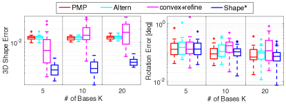
Figure 1: 3D shape estimation error (left) and rotation estimation error (right) by Shape^⋆ compared with PMP [36], Altern [49] and convex+refine [50], for increasing basis shapes $K=5,10,20$.

7.3 Shape${\#}$ for Robust Reconstruction

This section shows that Shape${\#}$ achieves state-of-the-art performance on the FG3DCar [26] dataset. The FG3DCar dataset contains 300 car images with ground-truth 2D landmarks ${\bm{Z}}\in{{\mathbb{R}}^{2\times N}},N=256$. It also contains $K=15$ 3D mesh models of different cars $\{{\bm{B}}_{k}\}_{k=1}^{K}$. To generate outliers, we randomly change $10\%-70\%$ of the $N$ ground-truth 2D landmarks ${\bm{Z}}$ to be arbitrary positions inside the image. We then evaluate the robustness of Shape${\#}$ compared with two other robust methods based on the assumption of sparse outliers in [50]: (i) robustified alternative optimization (label: Altern+Robust) and (ii) robustified convex optimization (label: Convex+Robust). Fig. 2 boxplots the shape estimation and rotation estimation error under increasing outlier rates computed over 40 randomly chosen images in the FG3DCar dataset. We can see that Shape${\#}$ is insensitive to $70\%$ outliers, while the accuracy of both Altern+Robust and Convex+Robust decreases with respect to higher outlier rates and they fail at $60\%$ outliers. Fig. 3 shows two examples of qualitative results, where we see Shape${\#}$ gives high-quality model fitting at $70\%$ outliers, while the quality of Altern+Robust and Convex+Robust starts decreasing at $40\%$ outliers. More qualitative results are given in the Supplementary Material.

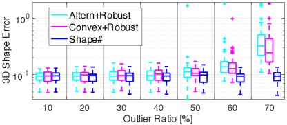
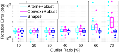
Figure 2: 3D shape estimation error (top) and rotation estimation error (bottom) by Shape${\#}$ compared with Altern+Robust [50] and Convex+Robust [50] under increasing outlier rates.

Altern+Robust	Convex+Robust	Shape${\#}$
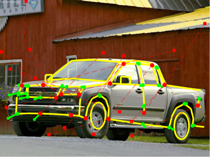
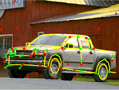
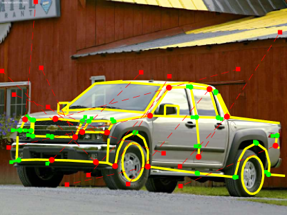
(a) Chevrolet Colorado LS $40\%$ outliers.
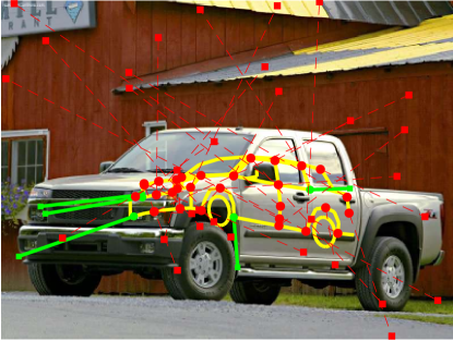
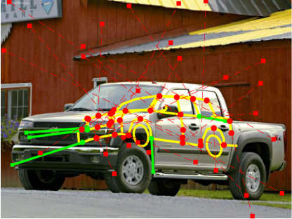
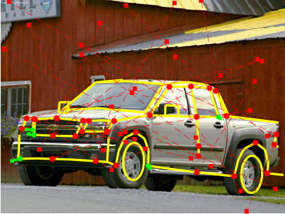
(b) Chevrolet Colorado LS $70\%$ outliers.
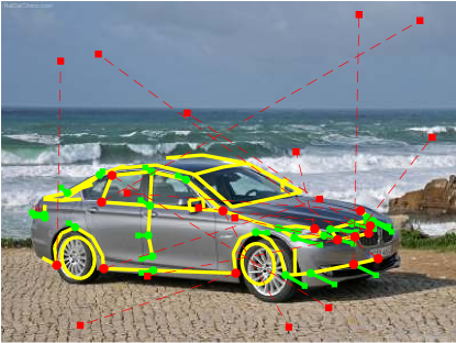
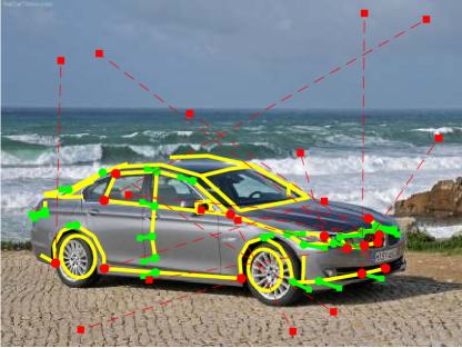
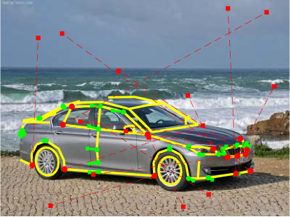
(c) BMW 5-Series $40\%$ outliers.
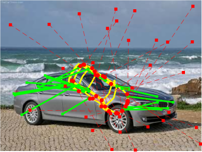
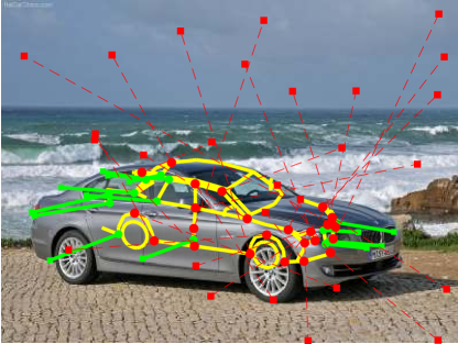
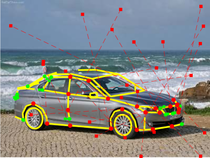
(d) BMW 5-Series $70\%$ outliers.

Figure 3: Selected qualitative results on the FG3DCar dataset [26] under $40\%$ and $70\%$ outlier rates using Altern+Robust [50], Convex+Robust [50], and Shape${\#}$. (a)-(b): results on the Chevrolet Colorado LS; (c)-(d): results on the BMW 5-Series. Green: inliers. Red: outliers. Circle: 3D landmark. Square: 2D landmark. [Best viewed electronically.]

8 Conclusions

We presented Shape^⋆, the first certifiably optimal solver for 3D shape reconstruction from 2D landmarks in a single image. Shape^⋆ is developed by applying Lasserre’s hierarchy of SOS relaxations combined with basis reduction to improve efficiency. Experimental results show that the SOS relaxation of order 2 always achieves global optimality. To handle outlying measurements, we also proposed Shape${\#}$, which solves a truncated least squares robust estimation problem by iteratively running Shape^⋆ without the need for an initial guess. We show that Shape${\#}$ achieves robustness against $70\%$ outliers on the FG3DCar dataset and outperforms state-of-the-art solvers.

Supplementary Material

9 Proof of Theorem 4

Proof.

Here we prove Theorem 4 in the main document. Recall the weighted least squares optimization for shape reconstruction in eq. (13) and denote its objective function as $f(\bm{c},{\bm{R}},\bm{t})$, with $\bm{c}=[c_{1},\dots,c_{k}]^{\mathsf{T}}$:

$$f(\bm{c},{\bm{R}},\bm{t})=\\ \displaystyle\sum_{i=1}^{N}w_{i}\left\|\bm{z}_{i}-\Pi{\bm{R}}\left(\sum_{k=1}^{K}c_{k}{\bm{B}}_{ki}\right)-\bm{t}\right\|^{2}+\alpha\sum_{k=1}^{K}\left|c_{k}\right|.$$ (A1)

In order to marginalize out the translation $\bm{t}$, we compute the derivative of $f(\bm{c},{\bm{R}},\bm{t})$ w.r.t. $\bm{t}$:

$$\frac{\partial f}{\partial\bm{t}}=2\sum_{i=1}^{N}w_{i}\bm{t}-2\sum_{i=1}^{N}w_{i}\left(\bm{z}_{i}-\Pi{\bm{R}}\left(\sum_{k=1}^{K}c_{k}{\bm{B}}_{ki}\right)\right),$$ (A2)

and set it to $\bm{0}$, which allows us to write $\bm{t}^{\star}$ in closed form using ${\bm{R}}^{\star}$ and $\bm{c}^{\star}$:

$$\bm{t}^{\star}=\bar{\bm{z}}^{w}-\Pi{\bm{R}}^{\star}\left(\sum_{k=1}^{K}c_{k}^{\star}\bar{{\bm{B}}}^{w}_{k}\right),$$ (A3)

with $\bar{\bm{z}}^{w}$ and $\bar{{\bm{B}}}^{w}_{k},k=1,\dots,K,$ being the weighted centers of the 2D landmarks ${\bm{Z}}$ and the 3D basis shapes ${\bm{B}}_{k}$:

$$\bar{\bm{z}}^{w}=\frac{\sum_{i=1}^{N}w_{i}\bm{z}_{i}}{\sum_{i=1}^{N}w_{i}},\quad\bar{{\bm{B}}}^{w}_{k}=\frac{\sum_{i=1}^{N}\bar{{\bm{B}}}_{ki}}{\sum_{i=1}^{N}w_{i}}.$$ (A4)

Then we can substitute the expression of $\bm{t}^{\star}$ in (A3) back into the objective function in (A1) and obtain an objective function without translation:

$$f^{\prime}(\bm{c},{\bm{R}})=\\ \sum_{i=1}^{N}w_{i}\left\|(\bm{z}_{i}-\bar{\bm{z}}^{w})-\Pi{\bm{R}}\left(\sum_{k=1}^{K}c_{i}({\bm{B}}_{ik}-\bar{{\bm{B}}}^{w}_{k})\right)\right\|^{2}+\\ \alpha\sum_{k=1}^{K}|c_{k}|$$ (A5)

Lastly, by defining:

$$\tilde{\bm{z}}_{i}=\sqrt{w_{i}}(\bm{z}_{i}-\bar{\bm{z}}^{w}),$$ (A6)

$$\tilde{{\bm{B}}}_{ki}=\sqrt{w_{i}}({\bm{B}}_{ki}-\bar{{\bm{B}}}^{w}),k=1,\dots,K$$ (A7)

we can see the equivalence between the objective function in eq. (A5) and the objective function in eq. (14) of Theorem 4. The constraints remain unchanged because we only marginalize out the unconstrained variable $\bm{t}$. Therefore, the shape reconstruction problem (13) is equivalent to the translation-free problem (14), and the optimal translation can be recovered using eq. (A3). ∎

10 Proof of Proposition 6

Proof.

Here we prove the SOS relaxation of order $\beta$ ($\beta\geq 2$) for the translation-free shape reconstruction problem (14) is the semidefinite program in (22). First, let us rewrite the general form of Lasserre’s hierarchy of order $\beta$ in eq. (8) in Theorem 3 as the following:

$$\max \gamma$$ (A8)

$$s.t. f(\bm{x})-\gamma=h+g,$$

$$h\in\langle\bm{h}\rangle_{2\beta},$$

$$g\in Q_{\beta}(\bm{g}).$$

In words, the constraints of (A8) ask the polynomial $f(\bm{x})-\gamma$ to be written as a sum of two polynomials $h$ and $g$, with $h$ in the $2\beta$-th truncated ideal of $\bm{h}$, and $g$ in the $\beta$-th truncated quadratic module of $\bm{g}$.

Next, we use the definition of the $2\beta$-th truncated ideal and the $\beta$-th truncated quadratic module to explicitly represent $h$ and $g$. First recall the definition of the $2\beta$-th truncated ideal in eq. (5), which states that $h$ must be written as a sum of polynomial products between the equality constraints $h_{i}$’s and the polynomial multipliers $\lambda_{i}$’s:

$$h=\sum_{i=1}^{15}\lambda_{i}h_{i},$$ (A9)

and the degree of each polynomial product $\lambda_{i}h_{i}$ must be no greater than $2\beta$, i.e., $\deg(\lambda_{i}h_{i})\leq 2\beta$. In the translation-free shape reconstruction problem, because all the 15 equality constraints in eq. (19) (arising from ${\bm{R}}\in\mathrm{SO}(3)$) have degree 2, the degree of the polynomial multipliers must be at most $2\beta-2$, i.e., $\deg(\lambda_{i})\leq 2\beta-2$. Therefore, we can parametrize each $\lambda_{i}$ using $[\bm{x}]_{2\beta-2}$, the vector of monomials up to degree $2\beta-2$:

$$\lambda_{i}=\bm{\lambda}_{i}^{\mathsf{T}}[\bm{x}]_{2\beta-2},\quad\bm{\lambda}_{i}\in{{\mathbb{R}}^{N_{\lambda}}},N_{\lambda}=\left(\begin{subarray}{c}K+7+2\beta\\ 2\beta-2\end{subarray}\right),$$ (A10)

with $\bm{\lambda}_{i}$ being the vector of unknown coefficients associated with the monomial basis $[\bm{x}]_{2\beta-2}$. The size of $\bm{\lambda}_{i}$ is equal to the length of $[\bm{x}]_{2\beta-2}$, which can be computed by $\left(\begin{subarray}{c}n+d\\ d\end{subarray}\right)$, with $n=K+9$ being the number of variables in $\bm{x}$, and $d=2\beta-2$ being the maximum degree of the monomial basis. Similarly for $g$, we recall the definition of the $\beta$-th truncated quadratic module in eq. (7), which states that $g$ must be written as a sum of polynomial products between the inequality constraints $g_{k}$’s and the SOS polynomial multipliers $s_{k}$’s:

$$g=\sum_{k=0}^{2K}s_{k}g_{k},$$ (A11)

and the degree of each polynomial product $s_{k}g_{k}$ must be no greater than $2\beta$, i.e., $\deg(s_{k}g_{k})\leq 2\beta$. For our specific shape reconstruction problem, we have $g_{0}:=1$, $g_{k}=c_{k},k=1,\dots,K$, and $g_{K+k}=1-c_{k}^{2},k=1,\dots,K$. Since $g_{0}$ has degree 0, $s_{0}$ can have degree up to $2\beta$. All $g_{k},k=1,\dots,K$, have degree 1, so $s_{k},k=1,\dots,K$, can have degree up to $2\beta-1$. However, because SOS polynomials can only have even degree, $s_{k},k=1,\dots,K$ can only have degree up to $2\beta-2$. For $g_{K+k},k=1,\dots,K$, they have degree 2, so their corresponding SOS polynomial multipliers $s_{K+k},k=1,\dots,K$ can have degree up to $2\beta-2$. Now for each SOS polynomial $s_{k},k=0,\dots,2K$, from the Gram matrix representation in eq. (2), we can associate a PSD matrix ${\bm{S}}_{k}$ with it using corresponding monomial bases:

$$\begin{cases}s_{0}=[\bm{x}]_{\beta}^{\mathsf{T}}{\bm{S}}_{0}[\bm{x}]_{\beta}&{\bm{S}}_{0}\in{\cal S}_{+}^{N_{0}},N_{0}=\left(\begin{subarray}{c}K+9+\beta\\ \beta\end{subarray}\right)\\ s_{k\neq 0}=[\bm{x}]_{\beta-1}^{\mathsf{T}}{\bm{S}}_{k}[\bm{x}]_{\beta-1}&{\bm{S}}_{k}\in{\cal S}_{+}^{N_{\lambda}},N_{\lambda}=\left(\begin{subarray}{c}K+8+\beta\\ \beta-1\end{subarray}\right)\end{cases}$$ (A12)

Finally, by inserting the expressions of $s_{k}$ in (A12) back to the expression of $g$ in (A11), and inserting the expression of $\lambda_{i}$ in (A10) back to the expression of $h$ in (A9), we can convert the SOS relaxation of general form (A8) to the semidefinite program (22). ∎

11 Proof of Theorem 8

Proof.

According to [23], the dual SDP of (22) is the following SDP:

$$\min_{\bm{y}} L_{\bm{y}}(f)$$ (A13)

$$s.t. {\bm{M}}_{\beta}(\bm{y})\succeq 0,$$ (A14)

$${\bm{M}}_{\beta-v_{k}}(g_{k}\bm{y})\succeq 0,$$ (A15)

$${\bm{M}}_{\beta-u_{i}}(h_{i}\bm{y})={\mathbf{0}},$$ (A16)

$$y_{{\mathbf{0}}}=1,$$ (A17)

where $\bm{y}\in{{\mathbb{R}}^{N_{2\beta}}}$, $N_{2\beta}=\left(\begin{subarray}{c}K+9+2\beta\\ 2\beta\end{subarray}\right)$ is a vector of moments for a probability measure supported on ${\cal X}$ defined by the equalities $h_{i}$ and inequalities $g_{k}$; $L_{\bm{y}}(f)=\sum_{\bm{\alpha}}f_{\bm{\alpha}}y_{\bm{\alpha}}$ is a linear function of $\bm{y}$, where $f_{\bm{\alpha}}$ is the coefficient of $f(\bm{x})$ associated with monomial $\bm{x}^{\bm{\alpha}}$, and $y^{\bm{\alpha}}$ is the moment of the monomial $\bm{x}^{\bm{\alpha}}$ w.r.t. the probability measure; ${\bm{M}}_{\beta}(\bm{y})\in{{\mathbb{R}}^{N_{\beta}}},N_{\beta}=\left(\begin{subarray}{c}K+9+\beta\\ \beta\end{subarray}\right)$ is the moment matrix of degree $\beta$ that assembles all the moments in $\bm{y}$; ${\bm{M}}_{\beta-v_{k}}(g_{k}\bm{y}),v_{k}=\lceil\deg(g_{k})/2\rceil$, is the localizing matrix that takes some moments from the moment matrix ${\bm{M}}_{\beta}(\bm{y})$ and entry-wise multiply them with the inequality $g_{k}$ (cf. [23] for more details); ${\bm{M}}_{\beta-u_{i}}(h_{i}\bm{y}),u_{i}=\lceil\deg(h_{i})/2\rceil$ is the localizing matrix that takes some moments from the moment matrix and entry-wise multiply them with the equality $h_{i}$. Due to strong duality of the primal-dual SDP, we have complementary slackness:

$${\bm{S}}_{0}^{\beta\star}{\bm{M}}_{\beta}^{\star}={\mathbf{0}},$$ (A18)

at global optimality of the SDP pair. Since $\text{corank}({\bm{S}}_{0}^{\beta\star})=1$, then according to Theorem 5.7 of [23], we have $\mathrm{rank}\left({\bm{M}}_{\beta}^{\star}\right)=1$ and $f_{\beta}^{\star}$ is the global minimum of the original shape reconstruction problem (14). Further, as $\mathrm{rank}\left({\bm{M}}_{\beta}^{\star}\right)=1$, ${\bm{M}}_{\beta}^{\star}=\bm{v}^{\star}(\bm{v}^{\star})^{\mathsf{T}}$ where $\bm{v}^{\star}=[\bm{x}^{\star}]_{\beta}$ and $\bm{x}^{\star}$ is the unique global minimizer of the original problem (14). However, the fact that ${\bm{S}}_{0}^{\beta\star}{\bm{M}}_{\beta}^{\star}={\mathbf{0}}$ and ${\bm{M}}_{\beta}^{\star}=\bm{v}^{\star}(\bm{v}^{\star})^{\mathsf{T}}$ implies:

$${\bm{S}}_{0}^{\beta\star}\bm{v}^{\star}={\mathbf{0}},$$ (A19)

and $\bm{v}^{\star}$ is in the null-space of ${\bm{S}}_{0}^{\beta\star}$. Therefore, the solution extracted using Proposition 7 is also the unique global minimizer of problem (14). ∎

12 Derivation of Proposition 9

Here we show the intuition for using the basis reduction in Proposition 9. In the original SOS relaxation (22), the parametrization of the SOS polynomial multipliers $s_{k},k=0,\dots,2K$, and the polynomial multipliers $\lambda_{i},i=1,\dots,15$, uses the vector of all monomials up to their corresponding degrees (cf. (A10) and (A12)), which leads to an SDP of size $N_{0}=\left(\begin{subarray}{c}K+9+\beta\\ \beta\end{subarray}\right)$ that grows quadratically with the number of basis shapes $K$. In basis reduction, we do not limit ourselves to the vector of full monomials, but rather parametrize $s_{0}$, $s_{k}$ and $\lambda_{i}$ with unknown monomials bases $v_{0}[\bm{x}]$, $v_{s}[\bm{x}]$ and $v_{\lambda}[\bm{x}]$, which allows us to rewrite (23) as:

$$f(\bm{x})-\gamma=\overbrace{v_{0}[\bm{x}]^{\mathsf{T}}{\bm{S}}_{0}v_{0}[\bm{x}]}^{s_{0}}+\\ \sum_{k=1}^{2K}\overbrace{\left(v_{s}[\bm{x}]^{\mathsf{T}}{\bm{S}}_{k}v_{k}[\bm{x}]\right)}^{s_{k}}g_{k}(\bm{x})+\\ \sum_{i=1}^{15}\overbrace{\left(\bm{\lambda}_{i}^{\mathsf{T}}v_{\lambda}[\bm{x}]\right)}^{\lambda_{i}}h_{i}(\bm{x}),$$ (A20)

with the hope that $v_{0}[\bm{x}]\subseteq[\bm{x}]_{2}$, $v_{s}[\bm{x}]\subseteq[\bm{x}]_{1}$ and $v_{\lambda}[\bm{x}]\subseteq[\bm{x}]_{2}$ have much smaller sizes (we limit ourselves to the case of $\beta=2$, at which level the relaxation is empirically tight).

As described, one can see that the problem of finding smaller $v_{0}[\bm{x}]$, $v_{s}[\bm{x}]$ and $v_{\lambda}[\bm{x}]$, while keeping the relaxation empirically tight, is highly combinatorial in general. Therefore, our strategy is to only consider the following case:

1. Expressive: choose $v_{0}[\bm{x}]$ such that $s_{0}$ contains all the monomials in $f(\bm{x})-\gamma$,

2. Balanced: choose $v_{s}[\bm{x}]$ and $v_{\lambda}[\bm{x}]$ such that the sum $s_{0}+\sum s_{k}g_{k}+\sum\lambda_{i}h_{i}$ can only have monomials from $f(\bm{x})-\gamma$.

In words, condition (i) ensures that the right-hand side (RHS) of (A20) contains all the monomials of the left-hand side (LHS). Condition (ii) asks the three terms of the RHS, i.e., $s_{0}$, $\sum s_{k}g_{k}$ and $\sum\lambda_{i}h_{i}$, to be self-balanced in the types of monomials. For example, if $s_{0}$ contains extra monomials that are not in the LHS, then those extra monomials better appear also in $\sum s_{k}g_{k}$ and/or $\sum\lambda_{i}h_{i}$ so that they could be canceled by summation. Under these two conditions, it is possible to have equation (A20) hold.

The choices in both conditions depend on analyzing the monomials in $f(\bm{x})-\gamma$. Recall the expression of $f(\bm{x})$ in (14) and the expression $q_{i}(\bm{x})$ in (18) for each term inside the summation, it can be seen that $f(\bm{x})$ only contains the following types of monomials:

$$1$$ (A21)

$$c_{k},1\leq k\leq K$$ (A22)

$$c_{k}r_{j},1\leq k\leq K,1\leq j\leq 9$$ (A23)

$$c_{k_{1}}c_{k_{2}}r_{j_{1}}r_{j_{2}},1\leq k_{1}\leq k_{2}\leq K,1\leq j_{1}\leq j_{2}\leq 9$$ (A24)

and the key observation is that $f(\bm{x})$ does not contain degree-4 monomials purely in $\bm{c}$ or $\bm{r}$, i.e., $c_{k_{1}}c_{k_{2}}c_{k_{3}}c_{k_{4}}$ and $r_{j_{1}}r_{j_{2}}r_{j_{3}}r_{j_{4}}$, or any degree-3 monomials in $\bm{c}$ and $\bm{r}$. Therefore, when choosing $v_{0}[\bm{x}]$, we can exclude degree-2 monomials purely in $\bm{c}$ and $\bm{r}$ from $[\bm{x}]_{2}$, and set $v_{0}[\bm{x}]=m_{2}(\bm{x})=[1,\bm{c}^{\mathsf{T}},\bm{r}^{\mathsf{T}},\bm{c}^{\mathsf{T}}\otimes\bm{r}^{\mathsf{T}}]^{\mathsf{T}}$ as stated in Proposition 9. This will satisfy the expressive condition (i), because $s_{0}=m_{2}[\bm{x}]^{\mathsf{T}}{\bm{S}}_{0}m_{2}[\bm{x}]$ can have the following monomials:

$$1,\quad c_{k},\quad c_{k}r_{j},\quad c_{k_{1}}c_{k_{2}}r_{j_{1}}r_{j_{2}}$$ (A25)

$$r_{j},\quad c_{k_{1}}c_{k_{2}},\quad r_{j_{1}}r_{j_{2}},\quad c_{k_{1}}c_{k_{2}}r_{j},\quad c_{k}r_{j_{1}}r_{j_{2}}$$ (A26)

and those in (A25) cover the monomials in $f(\bm{x})$. Replacing $[\bm{x}]_{2}$ with $v_{0}[\bm{x}]=m_{2}(\bm{x})$ is the key step in reducing the size of the SDP, because it reduces the size of the SDP from $\left(\begin{subarray}{c}K+11\\ 2\end{subarray}\right)$ to $10K+10$, i.e., from quadratic to linear in $K$.

In order to satisfy condition (ii), when choosing $v_{s}[\bm{x}]$ and $v_{\lambda}[\bm{x}]$, the goal is to have the product between $s_{k}$, $\lambda_{i}$ and $g_{k}$, $h_{i}$ result in monomials that appear in $f(x)-\gamma$, and ensure that monomials that do not appear in the latter can simplify our in the summation. For example, as stated in Proposition 9, we choose $v_{s}[\bm{x}]=[\bm{r}]_{1}=[1,\bm{r}^{\mathsf{T}}]^{\mathsf{T}}$ and $s_{k}$ will contain monomials 1, $r_{j}$ and $r_{j_{1}}r_{j_{2}}$. Because $g_{k}$’s have monomials $1$, $c_{k}$ and $c_{k}^{2}$, we can see that $\sum s_{k}g_{k}$ will contain the following monomials:

$$1,\ c_{k},\ r_{j_{1}}r_{j_{2}}c_{k}^{2},$$ (A27)

$$c_{k}^{2},\ r_{j},\ r_{j}c_{k}^{2},\ r_{j_{1}}r_{j_{2}},\ r_{j_{1}}r_{j_{2}}c_{k},\$$ (A28)

This still satisfies the balanced condition, because monomials of $\sum s_{k}g_{k}$ in (A27) balance with monomials of $s_{0}$ in (A25), and monomials of $\sum s_{k}g_{k}$ in (A27) balance with monomials of $s_{0}$ in (A26). Similarly, choosing $v_{\lambda}[\bm{x}]=[\bm{c}]_{2}$ makes $\lambda_{i}$ have monomials $1$, $c_{k}$ and $c_{k_{1}}c_{k_{2}}$, and because $h_{i}$’s have monomials $1$, $r_{j}$ and $r_{j_{1}}r_{j_{2}}$, we see that $\sum\lambda_{i}h_{i}$ contains the following monomials:

$$1,\ c_{k},\ c_{k}r_{j},\ c_{k_{1}}c_{k_{2}}r_{j_{1}}r_{j_{2}},$$ (A29)

$$r_{j},\ r_{j_{1}}r_{j_{2}},\ c_{k}r_{j_{1}}r_{j_{2}},\ c_{k_{1}}c_{k_{2}},\ c_{k_{1}}c_{k_{2}}r_{j},$$ (A30)

which balance with monomials in $s_{0}$ from (A25) and (A26).

We remark that we cannot guarantee that the SOS relaxation resulting from basis reduction can achieve the same performance as the original SOS relaxation and we cannot guarantee our choice of basis is “optimal” in any sense. Therefore, in practice, one needs to check the solution and compute $\text{corank}({\bm{S}}_{0}^{2\star})$ and $\eta_{2}$ to check the optimality of the solution produced by (27). Moreover, it remains an open problem to find a better set of monomials bases to achieve better reduction (e.g., knowing more about the algebraic geometry of $g_{k}$ and $h_{i}$ could possibly enable using the standard monomials as a set of bases [6]).

13 Derivation of Algorithm 1

For a complete discussion of graduated non-convexity and its applications for robust spatial perception, please see [45].

In the main document, for robust shape reconstruction, we adopt the TLS shape reconstruction formulation:

$$\!\!\!\min_{\begin{subarray}{c}c_{k}\geq 0,\\ k=1,\dots,K\\ \bm{t}\in{{\mathbb{R}}^{2}},{\bm{R}}\in\mathrm{SO}(3)\end{subarray}} \displaystyle\sum_{i=1}^{N}\rho_{\bar{c}}\left(r_{i}(c_{k},{\bm{R}},\bm{t})\right)+\alpha\!\sum_{k=1}^{K}\!c_{k}$$ (A31)

where $r_{i}(c_{k},{\bm{R}},\bm{t}):=\left\|\bm{z}_{i}\!-\!\Pi{\bm{R}}\left(\sum_{k=1}^{K}c_{k}{\bm{B}}_{ki}\right)\!-\!\bm{t}\right\|$ is called the residual, and $\rho_{\bar{c}}(r)=\min(r^{2},\bar{c}^{2})$ implements a truncated least squares cost. Recalling that $\rho_{\bar{c}}(r)=\min(r^{2},\bar{c}^{2})=\min_{w\in\{0,1\}}wr^{2}+(1-w)\bar{c}^{2}$, we can rewrite the TLS shape reconstruction as a joint optimization of $(\bm{c},{\bm{R}},\bm{t})$ and the binary variables $w_{i}$’s, as in eq. (30) in the main document. However, as hinted in the main document, due to the non-convexity of the TLS cost, directly solving the joint problem or alternating between solving for $(\bm{c},{\bm{R}},\bm{t})$ and binary variables $w_{i}$’s would require an initial guess and is prone to bad local optima.

The idea of graduated non-convexity (GNC) [4] is to introduce a surrogate function $\rho^{\mu}_{\bar{c}}(r)$, governed by a control parameter $\mu$, such that changing $\mu$ allows $\rho^{\mu}_{\bar{c}}(r)$ to start from a convex proxy of $\rho_{\bar{c}}(r)$, and gradually increase the amount of non-convexity till the original TLS function $\rho_{\bar{c}}(r)$ is recovered. The surrogate function for TLS is stated below.

Proposition A1 (Truncated Least Squares (TLS) and GNC).

The truncated least squares function is defined as:

$$\rho_{\bar{c}}(r)=\begin{cases}\scriptstyle{r^{2}}&{\footnotesize\text{ if }}\scriptstyle{r^{2}\in\left[0,\bar{c}^{2}\right]}\\ \scriptstyle{\bar{c}^{2}}&{\footnotesize\text{ if }}\scriptstyle{r^{2}\in\left[\bar{c}^{2},+\infty\right)}\end{cases},$$ (A32)

where $\bar{c}$ is a given truncation threshold. The GNC surrogate function with control parameter $\mu$ is:

$$\rho^{\mu}_{\bar{c}}(r)=\begin{cases}\scriptstyle{r^{2}}&{\footnotesize\text{ if }}\scriptstyle{r^{2}\in\left[0,\frac{\mu}{\mu+1}\bar{c}^{2}\right]}\\ \scriptstyle{2\bar{c}|r|\sqrt{\mu(\mu+1)}-\mu(\bar{c}^{2}+r^{2})}&{\footnotesize\text{ if }}\scriptstyle{r^{2}\in\left[\frac{\mu}{\mu+1}\bar{c}^{2},\frac{\mu+1}{\mu}\bar{c}^{2}\right]}\\ \scriptstyle{\bar{c}^{2}}&{\footnotesize\text{ if }}\scriptstyle{r^{2}\in\left[\frac{\mu+1}{\mu}\bar{c}^{2},+\infty\right)}\end{cases}.$$ (A33)

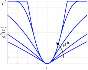
Figure A1: Graduated Non-Convexity (GNC) with control parameter $\mu$ for the Truncated Least Squares (TLS) cost.

By inspection, one can verify $\rho^{\mu}_{\bar{c}}(r)$ is convex for $\mu$ approaching zero (($\rho^{\mu}_{\bar{c}}(r))^{\prime\prime}=-2\mu\rightarrow 0$) and retrieves $\rho_{\bar{c}}(r)$ in (A32) for $\mu\rightarrow+\infty$. An illustration of $\rho^{\mu}_{\bar{c}}(r)$ is given in Fig. A1.

The nice property of the GNC surrogate function is that when $\mu$ is close to zero, $\rho^{\mu}_{\bar{c}}$ is convex, which means the only non-convexity of problem (A31) comes from the constraints and can be relaxed using the SOS relaxations.

For the GNC surrogate function $\rho^{\mu}_{\bar{c}}$, the simple trick of introducing binary variables ($\rho_{\bar{c}}(r)=\min_{w\in\{0,1\}}wr^{2}+(1-w)\bar{c}^{2}$) would not work. However, Black and Rangarajan [3] showed that this idea of introducing an outlier variable can be generalized to many robust cost functions. In particular, for the GNC surrogate function, we have the following.

Theorem A2 (Black-Rangarajan Duality for GNC surrogate TLS).

The GNC surrogate TLS shape reconstruction:

$$\!\!\!\min_{\begin{subarray}{c}c_{k}\geq 0,\\ k=1,\dots,K\\ \bm{t}\in{{\mathbb{R}}^{2}},{\bm{R}}\in\mathrm{SO}(3)\end{subarray}} \displaystyle\sum_{i=1}^{N}\rho_{\bar{c}}^{\mu}\left(r_{i}(c_{k},{\bm{R}},\bm{t})\right)+\alpha\!\sum_{k=1}^{K}\!c_{k}$$ (A34)

with $\rho^{\mu}_{\bar{c}}(r)$ defined in (A33), is equivalent to the following optimization with outlier variables $w_{i}$’s:

$$\!\!\!\min_{\begin{subarray}{c}c_{k}\geq 0,\\ k=1,\dots,K\\ \bm{t}\in{{\mathbb{R}}^{2}},{\bm{R}}\in\mathrm{SO}(3)\\ w_{i}\in[0,1],i=1,\dots,N\end{subarray}}\displaystyle\sum_{i=1}^{N}\left[w_{i}r_{i}^{2}(c_{k},{\bm{R}},\bm{t})+\Phi^{\mu}_{\bar{c}}(w_{i})\right]+\alpha\!\sum_{k=1}^{K}\!c_{k}$$ (A35)

where $\Phi^{\mu}_{\bar{c}}(w_{i})$ is the following outlier process:

$$\Phi^{\mu}_{\bar{c}}(w_{i})=\frac{\mu(1-w_{i})}{\mu+w_{i}}\bar{c}^{2}.$$ (A36)

Proof.

The derivation of $\Phi^{\mu}_{\bar{c}}(w_{i})$ in (A36) follows the Black-Rangarajan procedure in Fig. 10 of [3]. ∎

In words, the Black-Rangarajan duality allows us to rewrite the non-convex shape reconstruction problem as a joint optimization in $(\bm{c},{\bm{R}},\bm{t})$ and outlier variables $w_{i}$’s. The interested readers can find closed-form outlier processes for many other robust cost functions in the original paper [3].

Leveraging the Black-Rangarajan duality, for any given choice of the control parameter $\mu$, we can solve problem (A35) in two steps: first we solve $(\bm{c},{\bm{R}},\bm{t})$ using Shape^⋆ with fixed weights $w_{i}$’s, and then we update the weights with fixed $(\bm{c},{\bm{R}},\bm{t})$. In particular, at each iteration $\tau$ (corresponding to a given control parameter $\mu$), we perform the following:

1. Variable update: minimize (A35) with respect to $(\bm{c},{\bm{R}},\bm{t})$, with fixed weights $w_{i}^{(\tau-1)}$:

   $$c_{k}^{(\tau)},{\bm{R}}^{(\tau)},\bm{t}^{(\tau)}=\\ \!\!\!\operatorname*{arg\,min}_{\begin{subarray}{c}c_{k}\geq 0,\\ k=1,\dots,K\\ \bm{t}\in{{\mathbb{R}}^{2}},{\bm{R}}\in\mathrm{SO}(3)\end{subarray}}\displaystyle\sum_{i=1}^{N}w_{i}^{(\tau-1)}r_{i}^{2}(c_{k},{\bm{R}},\bm{t})+\alpha\!\sum_{k=1}^{K}\!c_{k},$$ (A37)

   where we have dropped the term $\sum_{i=1}^{N}\Phi^{\mu}_{\bar{c}}(w_{i})$ because it is independent from $(\bm{c},{\bm{R}},\bm{t})$. This problem is exactly the weighted least squares problem (13) and can be solved using Shape^⋆ (cf. line 1 in Algorithm 1). Using the solutions $(c_{k}^{(\tau)},{\bm{R}}^{(\tau)},\bm{t}^{(\tau)})$, we can compute the residuals $r_{i}^{(\tau)}$ (cf. line 1 in Algorithm 1).

2. Weight update: minimize (A35) with respect to $w_{i}$, with fixed residuals $r_{i}^{(\tau)}$:

   $$w_{i}^{(\tau)}=\operatorname*{arg\,min}_{w_{i}\in[0,1],i=1,\dots,N}\sum_{i=1}^{N}(r_{i}^{(\tau)})^{2}w_{i}+\Phi_{\bar{c}}^{\mu}(w_{i}),$$ (A38)

   where we have dropped $\sum_{k=1}^{K}c_{k}^{(\tau)}$ because it is a constant for the optimization. This optimization, fortunately, can be solved in closed-form. We take the gradient of the objective function with respect to $w_{i}$:

   $$\nabla_{w_{i}}=(r_{i}^{(\tau)})^{2}+\nabla_{w_{i}}\Phi_{\bar{c}}^{\mu}(w_{i})$$

   $$=(r_{i}^{(\tau)})^{2}-\frac{\mu(\mu+1)}{(\mu+w_{i})^{2}}\bar{c}^{2}$$ (A39)

   and observe that $\nabla_{w_{i}}=(r_{i}^{(\tau)})^{2}-\frac{\mu+1}{\mu}\bar{c}^{2}$ when $w_{i}=0$, and $\nabla_{w_{i}}=(r_{i}^{(\tau)})^{2}-\frac{\mu}{\mu+1}\bar{c}^{2}$ when $w_{i}=1$. Therefore, the global minimizer $w_{i}^{\star}:=w_{i}^{(\tau)}$ is:

   $${}w_{i}^{(\tau)}=\begin{cases}0&\text{ if }(r_{i}^{(\tau)})^{2}\in\left[\frac{\mu+1}{\mu}\bar{c}^{2},+\infty\right]\\ \frac{\bar{c}}{r_{i}^{(\tau)}}\sqrt{\mu(\mu+1)}-\mu&\text{ if }(r_{i}^{(\tau)})^{2}\in\left[\frac{\mu}{\mu+1}\bar{c}^{2},\frac{\mu+1}{\mu}\bar{c}^{2}\right]\\ 1&\text{ if }(r_{i}^{(\tau)})^{2}\in\left[0,\frac{\mu}{\mu+1}\bar{c}^{2}\right]\end{cases}.$$ (A40)

   and this is the weight update rule in line 1 of Algorithm 1.

After both the variables and weights are updated using the shaperobust approach described above, we increase the control parameter $\mu$ to increase the non-convexity of the surrogate function $\rho^{\mu}_{\bar{c}}$ (cf. line 1 of Algorithm 1). At the next iteration $\tau+1$, the updated weights are used to perform the variable update. The iterations terminate when the change in the objective function becomes negligible (cf. line 1 of Algorithm 1) or after a maximum number of iterations (cf. line 1 of Algorithm 1). Note that all weights are initialized to $1$ (cf. line 1 in Algorithm 1), which means that initially all measurements are tentatively accepted as inliers, therefore no prior information about inlier/outlier is required.

14 FG3DCar Qualitative Results

Fig. 14 shows 9 full qualitative results comparing the performances of Altern+Robust [50], Convex+Robust [50] and Shape${\#}$ on the FG3DCar [26] dataset under $10\%$ to $70\%$ outlier rates. One can further see that the performance of Shape${\#}$ is sensitive to $70\%$ outliers, while the performances of Altern+Robust and Convex+Robust gradually degrade and fail at $50\%$ to $60\%$ outliers.

	$10\%$	$20\%$	$30\%$	$40\%$	$50\%$	$60\%$	$70\%$
Altern+Robust
Convex+Robust
Shape${\#}$
Chevrolet Colorado LS

Altern+Robust

& Convex+Robust Shape${\#}$    BMW 5-Series    Altern+Robust Convex+Robust Shape${\#}$    Mercedes-Benz C 600

Figure A2: Qualitative results on the FG3DCar dataset [26] under $10-70\%$ outlier rates using Altern+Robust [50], Convex+Robust [50], and Shape${\#}$. Yellow: shape reconstruction result projected onto the image. Green: inliers. Red: outliers. Circle: 3D landmark. Square: 2D landmark. [Best viewed electronically.]

& Convex+Robust Shape${\#}$    Honda CRV    Altern+Robust Convex+Robust Shape${\#}$    Mercedes-Benz GL450

Figure A2: Qualitative results on the FG3DCar dataset [26] under $10-70\%$ outlier rates using Altern+Robust [50], Convex+Robust [50], and Shape${\#}$. Yellow: shape reconstruction result projected onto the image. Green: inliers. Red: outliers. Circle: 3D landmark. Square: 2D landmark. (cont.) [Best viewed electronically.]

& Convex+Robust Shape${\#}$    Volvo V70    Altern+Robust Convex+Robust Shape${\#}$    Saab 93

Figure A2: Qualitative results on the FG3DCar dataset [26] under $10-70\%$ outlier rates using Altern+Robust [50], Convex+Robust [50], and Shape${\#}$. Yellow: shape reconstruction result projected onto the image. Green: inliers. Red: outliers. Circle: 3D landmark. Square: 2D landmark. (cont.) [Best viewed electronically.]

References

- [1] MOSEK ApS. The MOSEK optimization toolbox for MATLAB manual. Version 8.1., 2017.
- [2] Mathieu Aubry, Daniel Maturana, Alexei A Efros, Bryan C Russell, and Josef Sivic. Seeing 3D chairs: exemplar part-based 2D-3D alignment using a large dataset of CAD models. In IEEE Conf. on Computer Vision and Pattern Recognition (CVPR), pages 3762–3769, 2014.
- [3] Michael J. Black and Anand Rangarajan. On the unification of line processes, outlier rejection, and robust statistics with applications in early vision. Intl. J. of Computer Vision, 19(1):57–91, 1996.
- [4] Andrew Blake and Andrew Zisserman. Visual reconstruction. MIT Press, 1987.
- [5] Volker Blanz and Thomas Vetter. Face recognition based on fitting a 3D morphable model. IEEE Trans. Pattern Anal. Machine Intell., 25(9):1063–1074, 2003.
- [6] Grigoriy Blekherman, Pablo A Parrilo, and Rekha R Thomas. Semidefinite optimization and convex algebraic geometry. SIAM, 2012.
- [7] Jesus Briales and Javier Gonzalez-Jimenez. Convex Global 3D Registration with Lagrangian Duality. In IEEE Conf. on Computer Vision and Pattern Recognition (CVPR), 2017.
- [8] Burer, Samuel and Monteiro, Renato D C. A nonlinear programming algorithm for solving semidefinite programs via low-rank factorization. Mathematical Programming, 95(2):329–357, 2003.
- [9] Timothy F. Cootes, Christopher J. Taylor, David H. Cooper, and Jim Graham. Active shape models - their training and application. Comput. Vis. Image Underst., 61(1):38–59, January 1995.
- [10] Xiaochuan Fan, Kang Zheng, Youjie Zhou, and Song Wang. Pose locality constrained representation for 3D human pose reconstruction. In European Conf. on Computer Vision (ECCV), pages 174–188. Springer, 2014.
- [11] Lie Gu and Takeo Kanade. 3D alignment of face in a single image. In IEEE Conf. on Computer Vision and Pattern Recognition (CVPR), volume 1, pages 1305–1312, 2006.
- [12] Kaiming He, Georgia Gkioxari, Piotr Dollár, and Ross Girshick. Mask R-CNN. In Intl. Conf. on Computer Vision (ICCV), pages 2980–2988, 2017.
- [13] Mohsen Hejrati and Deva Ramanan. Analyzing 3D Objects in Cluttered Images. In Advances in Neural Information Processing Systems (NIPS), pages 593–601, 2012.
- [14] Didier Henrion, Jean-Bernard Lasserre, and Johan Löfberg. GloptiPoly 3: moments, optimization and semidefinite programming. Optim. Methods. Softw., 24(4-5):761–779, 2009.
- [15] Berthold K. P. Horn. Closed-form solution of absolute orientation using unit quaternions. J. Opt. Soc. Amer., 4(4):629–642, Apr 1987.
- [16] Fredrik Kahl and Didier Henrion. Globally optimal estimates for geometric reconstruction problems. Intl. J. of Computer Vision, 74(1):3–15, 2007.
- [17] Laurent Kneip, Hongdong Li, and Yongduek Seo. UPnP: An optimal o(n) solution to the absolute pose problem with universal applicability. In European Conf. on Computer Vision (ECCV), pages 127–142. Springer, 2014.
- [18] Nikos Kolotouros, Georgios Pavlakos, Michael J Black, and Kostas Daniilidis. Learning to reconstruct 3d human pose and shape via model-fitting in the loop. In Intl. Conf. on Computer Vision (ICCV), pages 2252–2261, 2019.
- [19] Nikos Kolotouros, Georgios Pavlakos, and Kostas Daniilidis. Convolutional mesh regression for single-image human shape reconstruction. In IEEE Conf. on Computer Vision and Pattern Recognition (CVPR), 2019.
- [20] Pierre-Yves Lajoie, Siyi Hu, Giovanni Beltrame, and Luca Carlone. Modeling perceptual aliasing in SLAM via discrete-continuous graphical models. IEEE Robotics and Automation Letters (RA-L), 2019.
- [21] Katrin Lasinger, René Ranftl, Konrad Schindler, and Vladlen Koltun. Towards robust monocular depth estimation: Mixing datasets for zero-shot cross-dataset transfer. arXiv preprint arXiv:1907.01341, 2019.
- [22] Jean B. Lasserre. Global optimization with polynomials and the problem of moments. SIAM J. Optim., 11(3):796–817, 2001.
- [23] Jean-Bernard Lasserre. Moments, positive polynomials and their applications, volume 1. World Scientific, 2010.
- [24] Monique Laurent. Sums of squares, moment matrices and optimization over polynomials. In Emerging applications of algebraic geometry, pages 157–270. Springer, 2009.
- [25] Yan Li, Leon Gu, and Takeo Kanade. Robustly aligning a shape model and its application to car alignment of unknown pose. IEEE transactions on pattern analysis and machine intelligence, 33(9):1860–1876, 2011.
- [26] Yen-Liang Lin, Vlad I. Morariu, Winston H. Hsu, and Larry S. Davis. Jointly optimizing 3D model fitting and fine-grained classification. In European Conf. on Computer Vision (ECCV), 2014.
- [27] Johan Löfberg. YALMIP: A toolbox for modeling and optimization in MATLAB. In Proceedings of the CACSD Conference, volume 3. Taipei, Taiwan, 2004.
- [28] Johan Lofberg. Pre-and post-processing sum-of-squares programs in practice. IEEE Transactions on Automatic Control, 54(5):1007–1011, 2009.
- [29] Anirudha Majumdar, Georgina Hall, and Amir Ali Ahmadi. A survey of recent scalability improvements for semidefinite programming with applications in machine learning, control, and robotics. arXiv preprint arXiv:1908.05209, 2019.
- [30] Joshua G Mangelson, Jinsun Liu, Ryan M Eustice, and Ram Vasudevan. Guaranteed globally optimal planar pose graph and landmark SLAM via sparse-bounded sums-of-squares programming. In IEEE Intl. Conf. on Robotics and Automation (ICRA), pages 9306–9312. IEEE, 2019.
- [31] Jiawang Nie. Optimality conditions and finite convergence of lasserre’s hierarchy. Mathematical programming, 146(1-2):97–121, 2014.
- [32] Frank Permenter and Pablo Parrilo. Partial facial reduction: simplified, equivalent SDPs via approximations of the PSD cone. 171(1-2):1–54, 2018.
- [33] Frank Permenter and Pablo A Parrilo. Basis selection for sos programs via facial reduction and polyhedral approximations. In 53rd IEEE Conference on Decision and Control, pages 6615–6620. IEEE, 2014.
- [34] Thomas Probst, Danda Pani Paudel, Ajad Chhatkuli, and Luc Van Gool. Convex relaxations for consensus and non-minimal problems in 3D vision. In Intl. Conf. on Computer Vision (ICCV), 2019.
- [35] Mihai Putinar. Positive polynomials on compact semi-algebraic sets. Indiana University Mathematics Journal, 42(3):969–984, 1993.
- [36] Varun Ramakrishna, Takeo Kanade, and Yaser Sheikh. Reconstructing 3D human pose from 2D image landmarks. In European Conf. on Computer Vision (ECCV), 2012.
- [37] David M Rosen, Luca Carlone, Afonso S Bandeira, and John J Leonard. SE-Sync: A certifiably correct algorithm for synchronization over the special Euclidean group. Intl. J. of Robotics Research, 38(2-3):95–125, 2019.
- [38] Denis Tome, Chris Russell, and Lourdes Agapito. Lifting from the deep: Convolutional 3d pose estimation from a single image. In IEEE Conf. on Computer Vision and Pattern Recognition (CVPR), pages 2500–2509, 2017.
- [39] Roberto Tron, David M Rosen, and Luca Carlone. On the inclusion of determinant constraints in lagrangian duality for 3D SLAM. In Robotics: Science and Systems (RSS), Workshop “The problem of mobile sensors: Setting future goals and indicators of progress for SLAM”.
- [40] Hayato Waki, Sunyoung Kim, Masakazu Kojima, and Masakazu Muramatsu. Sums of squares and semidefinite program relaxations for polynomial optimization problems with structured sparsity. SIAM J. Optim., 17(1):218–242, 2006.
- [41] Chunyu Wang, Yizhou Wang, Zhouchen Lin, Alan Loddon Yuille, and Wen Gao. Robust estimation of 3D human poses from a single image. In IEEE Conf. on Computer Vision and Pattern Recognition (CVPR), pages 2369–2376, 2014.
- [42] Tillmann Weisser, Jean B Lasserre, and Kim-Chuan Toh. Sparse-BSOS: a bounded degree SOS hierarchy for large scale polynomial optimization with sparsity. Math. Program. Comput., 10(1):1–32, 2018.
- [43] Jiajun Wu, Tianfan Xue, Joseph J Lim, Yuandong Tian, Joshua B Tenenbaum, Antonio Torralba, and William T Freeman. Single image 3d interpreter network. In European Conf. on Computer Vision (ECCV), pages 365–382. Springer, 2016.
- [44] Yu Xiang, Tanner Schmidt, Venkatraman Narayanan, and Dieter Fox. PoseCNN: A convolutional neural network for 6D object pose estimation in cluttered scenes. In Robotics: Science and Systems (RSS), 2018.
- [45] Heng Yang, Pasquale Antonante, Vasileios Tzoumas, and Luca Carlone. Graduated non-convexity for robust spatial perception: From non-minimal solvers to global outlier rejection. IEEE Robotics and Automation Letters (RA-L), 2020.
- [46] Heng Yang and Luca Carlone. A polynomial-time solution for robust registration with extreme outlier rates. In Robotics: Science and Systems (RSS), 2019.
- [47] Heng Yang and Luca Carlone. A quaternion-based certifiably optimal solution to the Wahba problem with outliers. In Intl. Conf. on Computer Vision (ICCV), 2019.
- [48] Heng Yang, Jingnan Shi, and Luca Carlone. TEASER: Fast and Certifiable Point Cloud Registration. arXiv preprint arXiv:2001.07715, 2020.
- [49] Xiaowei Zhou, Spyridon Leonardos, Xiaoyan Hu, and Kostas Daniilidis. 3D shape reconstruction from 2D landmarks: A convex formulation. In IEEE Conf. on Computer Vision and Pattern Recognition (CVPR), 2015.
- [50] Xiaowei Zhou, Menglong Zhu, Spyridon Leonardos, and Kostas Daniilidis. Sparse representation for 3D shape estimation: A convex relaxation approach. IEEE Trans. Pattern Anal. Machine Intell., 39(8):1648–1661, 2017.
- [51] Xiaowei Zhou, Menglong Zhu, Georgios Pavlakos, Spyridon Leonardos, Konstantinos G Derpanis, and Kostas Daniilidis. Monocap: Monocular human motion capture using a cnn coupled with a geometric prior. IEEE Trans. Pattern Anal. Machine Intell., 41(4):901–914, 2018.