Schmidt’s Game and Nonuniformly Expanding Interval Maps

Abstract.

We study Manneville–Pomeau maps on the unit interval and prove that the set of points whose forward orbits miss an interval with left endpoint 0 is strong winning for Schmidt’s game. Strong winning sets are dense, have full Hausdorff dimension, and satisfy a countable intersection property. Similar results were known for certain expanding maps, but these did not address the nonuniformly expanding case. Our analysis is complicated by the presence of infinite distortion and unbounded geometry.

1. Introduction and statement of results

Let $X$ be a compact metric space, $f$ a countably-branched piecewise-continuous map, and $\mu$ an $f$-invariant measure on $X$. There are broad conditions under which $\mu$-almost every point in $X$ has dense forward orbit under $f$. This is the case, for example, if $\mu$ is ergodic and fully supported on $X$. The “exceptional sets” of points with nondense orbits, despite being $\mu$-null, are nevertheless often large in a different sense. In particular they are often winning for Schmidt’s game, which implies that they are dense in $X$, have full Hausdorff dimension (if $X\subset\mathbb{R}^{n}$), and remain winning when intersected with countably many suitable winning sets in $X$. Examples of systems possessing winning exceptional sets include surjective endomorphisms of the torus [1, 2], beta transformations [3, 4], the Gauss map [5], and $C^{2}$ (uniformly) expanding maps of compact connected manifolds [6].

In this article we add to this list the Manneville–Pomeau map $f\colon\left[0,1\right]\to\left[0,1\right]$ defined by

$$f(x)=\begin{cases}x+x^{1+\gamma}&\text{if }0\leq x<r_{1}\\ x+x^{1+\gamma}-1&\text{if }r_{1}\leq x\leq 1,\end{cases}$$

where $\gamma>0$ is a fixed parameter and $r_{1}$ is the unique solution of $x+x^{1+\gamma}=1$ (see Figure 2). Our main result is the following theorem, which we prove in §7.

Theorem 1.1.

The set

$$\mathcal{E}_{f}:=\big{\{}x\in\left[0,1\right]\colon\left.\left[0,\epsilon\right.\right)\cap\left\{f^{n}x\right\}_{n\geq 0}=\emptyset\text{ for some }\epsilon>0\big{\}}$$

is strong winning for Schmidt’s game.

Remark 1.2.

As the proof of Theorem 1.1 will demonstrate, the strong winning dimension of $\mathcal{E}_{f}$, i.e., the supremum of all $\alpha$ for which $\mathcal{E}_{f}$ is $\alpha$-strong winning, depends on $\gamma$.

Remark 1.3.

It is well-known that $\operatorname{Leb}\left(\mathcal{E}_{f}\right)=0$. Indeed, we may express $\mathcal{E}_{f}$ as a countable union of nested Cantor sets:

$$\mathcal{E}_{f}=\bigcup_{n=1}^{\infty}\mathcal{C}_{n},\quad\mathcal{C}_{n}:=\bigcap_{k=0}^{\infty}f^{-k}\left(\left[r_{n},1\right]\right).$$

The sets $\mathcal{C}_{n}$ are compact and $f$-invariant. By suitably modifying $f$ on the interval $\left[0,r_{n}\right]$, the fact that $\operatorname{Leb}\left(\mathcal{C}_{n}\right)=0$ now follows from the standard result that compact sets invariant under a $C^{2}$ circle map are Lebesgue-null.

One consequence of Theorem 1.1 concerns the set $S$ of points having positive lower Lyapunov exponent for $f$. Recall that for $x\in\left[0,1\right]$ the lower Lyapunov exponent of $x$ is the number $\liminf_{n\to\infty}\frac{1}{n}\sum_{k=0}^{n-1}\log\big{|}\big{(}f^{k}\big{)}^{\prime}\left(x\right)\big{|}$ (using one-sided derivatives as necessary). We prove the following corollary in §4.

Corollary 1.4.

The set of points with positive lower Lyapunov exponent for $f$ is strong winning for Schmidt’s game.

It was known [7, 8] that $S$ has full Hausdorff dimension for all values of $\gamma>0$; Corollary 1.4 greatly strengthens this. In the case that $\gamma<1$, $f$ possesses a fully supported absolutely continuous (with respect to Lebesgue measure) ergodic probability measure $\mu$, so that Lebesgue-almost every point has positive lower Lyapunov exponent since $\operatorname{Lyap}(\mu)>0$ (see [9] and references therein). Note that even sets with full Lebesgue measure are not necessarily winning (the complement of a Legesgue-null winning set is never winning by Theorem 3.1 below; an example is the set of reals normal to a given base [5]). When $\gamma\geq 1$, however, $\operatorname{Leb}(S)=0$ [9], and so Corollary 1.4 is the strongest available result concerning the “largeness” of the set $S$ in this case, and gives another example of a Lebesgue-null winning set.

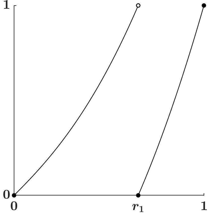
Figure 1. The graph of the Manneville–Pomeau map $f$ with $\gamma=1.5$.

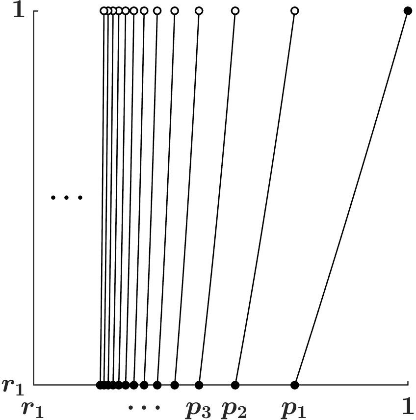
Figure 2. The graph of $F$, the first return map to $\left[r_{1},1\right]$ induced by $f$.

2. Method of proof

The primary difficulty in studying $f$ is the nonuniformity of expansion near the indifferent fixed point 0, which gives rise to infinite distortion. The map $f$ also exhibits unbounded geometry, by which we mean that the ratio of the longest to the shortest Markov partition element of successive generations tends to infinity. We address the problem of infinite distortion by inducing $f$ on $\left[r_{1},1\right]$ to get a uniformly expanding first return map $F$. This induced map satisfies a bounded distortion estimate, which is a key property of expanding systems that features prominently in the articles mentioned above. The issue of unbounded geometry is overcome using the notion of “commensurate,” introduced in [10].

The bulk of this paper involves analyzing the induced map $F\colon\left[r_{1},1\right]\to\left[r_{1},1\right]$ given by the rule

$$Fx:=f^{\tau\left(x\right)}\left(x\right),\quad\tau\left(x\right):=\min\left\{n\geq 0\colon f^{n}x\in\left[r_{1},1\right]\right\}.$$

See Figure 2. We will show that Theorem 1.1 is a straightforward consequence of the following analogous result for $F$, which we prove in §6:

Theorem 2.1.

The set

$$\mathcal{E}_{F}:=\left\{x\in\left[r_{1},1\right]\colon\left.\left[r_{1},r_{1}+\epsilon\right.\right)\cap\left\{F^{n}x\right\}_{n\geq 0}=\emptyset\text{ for some }\epsilon>0\right\}$$

is strong winning for Schmidt’s game.

Remark 2.2.

Our proof of Theorem 2.1 works for any map topologically conjugate to $F$ and satisfying the estimates concerning the Markov structure of $F$ in Proposition 4.9.

In proving Theorem 2.1 we follow the approach of Mance and Tseng in [10]. In that article the authors studied Lüroth expansions, whose associated dynamical system is piecewise linear. This linear structure permitted a precise computation of the lengths of intervals in the natural Markov partition. In this paper we cannot obtain closed-form expressions for these lengths; instead we derive estimates (Corollary 4.10) derived from a distortion result (Proposition 4.9).

We note that in [4] Hu and Yu considered the class of piecewise locally $C^{1+\delta}$ expanding maps, a class that includes the Gauss map. At first glance the induced map $F$ looks quite similar to the Gauss map; however, the authors in [4] required a Hölder-type distortion estimate that $F$ does not satisfy.

3. Schmidt’s Game

We describe a simplified version of a set-theoretic game introduced by Schmidt in [5]. The game is played on the unit interval $\left[0,1\right]$. Fix two constants $\alpha,\beta\in\left(0,1\right)$ and a set $S\subset\left[0,1\right]$. Two players, Alice and Bob, alternately choose nested closed intervals $B_{1}\supset A_{1}\supset B_{2}\supset A_{2}\supset\dots$ with Bob choosing first. These intervals must satisfy the relations $\left|B_{n+1}\right|=\beta\left|A_{n}\right|$ and $\left|A_{n}\right|=\alpha\left|B_{n}\right|$ for all $n\in\mathbb{N}$ ($\left|B_{1}\right|$ is arbitrary). Then $\bigcap A_{n}=\bigcap B_{n}$ consists of a single point, $\omega$. Alice wins the game if and only if $\omega\in S$.

If Alice has a winning strategy by which she can win regardless of Bob’s choices, $S$ is said to be $\left(\alpha,\beta\right)$-winning. $S$ is called $\alpha$-winning if it is $\left(\alpha,\beta\right)$-winning for all $\beta\in\left(0,1\right)$. $S$ is called winning if it is $\alpha$-winning for some $\alpha\in\left(0,1\right)$. The following result lists important properties of winning sets; the proof may be found in [5].

Theorem 3.1.

A winning set in $\left[0,1\right]$ is dense, uncountable, and has full Hausdorff dimension. A countable intersection of $\alpha$-winning sets is $\alpha$-winning. A cocountable subset of an $\alpha$-winning set is $\alpha$-winning.

In [11] McMullen introduced a modification of Schmidt’s game in which the length restrictions are loosened to $\left|B_{n+1}\right|\geq\beta\left|A_{n}\right|$ and $\left|A_{n}\right|\geq\alpha\left|B_{n}\right|$. This results in strong winning sets. As the name implies, strong winning sets are winning. In addition, the strong winning property is preserved under quasisymmetric homeomorphisms, which is not generally true of the winning property.

4. Proofs of Minor Results

4.1. Notation

Let $B\subset\left[0,1\right]$ be a closed interval. The expression $[B)$ denotes the interior of $J$ union its left endpoint; $(B]$ is similarly defined. $\partial^{\ell}B$ and $\partial^{r}B$ denote the left and right endpoints of $B$, respectively. The notations $\overline{B}$ and $B^{\circ}$ denote the closure and interior of $B$, respectively. $|B|$ denotes the diameter of $B$, and we call $B$ nontrivial if $0<|B|<1$. Henceforth all closed intervals are assumed to be nontrivial.

4.2. Technical results

Definition 4.1 (The sequence $\left\{r_{n}\right\}_{n=0}^{\infty}$).

Define $\left\{r_{n}\right\}_{n=0}^{\infty}\subset\left.\left(0,1\right.\right]$ recursively by $r_{0}=1$ and $\left\{r_{n+1}\right\}=f^{-1}\left(r_{n}\right)\cap\left(0,r_{n}\right)$; thus $r_{n}\searrow 0$.

Definition 4.2 (The sequence $\left\{p_{n}\right\}_{n=0}^{\infty}$).

Define $\left\{p_{n}\right\}_{n=0}^{\infty}\subset\left.\left(r_{1},1\right.\right]$ recursively by $p_{0}=1$ and $\left\{p_{n}\right\}:=f^{-1}\left(r_{n}\right)\cap\left(r_{1},1\right)$; thus $p_{n}\searrow r_{1}$.

The asymptotics of these sequences will play a crucial role. Proofs of the next two results may be found in §6.2 of [12].

Theorem 4.3 (The asymptotics of $\left\{r_{n}\right\}_{n=0}^{\infty}$).

There exists a constant $C_{1}>1$ such that for all $n\in\mathbb{N}$,

$$C_{1}^{-1}n^{-\frac{1}{\gamma}}\leq r_{n}\leq C_{1}n^{-\frac{1}{\gamma}},$$

$$C_{1}^{-1}n^{-1-\frac{1}{\gamma}}\leq r_{n-1}-r_{n}\leq C_{1}n^{-1-\frac{1}{\gamma}}.$$

Theorem 4.4 (A distortion estimate for $f\mathord{\upharpoonright}_{\left[0,r_{1}\right]}$).

There exists a constant $C_{2}>1$ such that for all integers $1\leq m\leq n$, and for all points $x,y\in\left.\left[r_{n+1},r_{n}\right.\right)$,

$$\left|\log\frac{\left(f^{m}\right)^{\prime}x}{\left(f^{m}\right)^{\prime}y}\right|\leq\frac{C_{2}}{r_{n-m}-r_{n-m+1}}\left|f^{m}x-f^{m}y\right|.$$

Corollary 4.5 (A distortion estimate for $f\mathord{\upharpoonright}_{\left[r_{1},1\right]}$).

There exists a constant $C_{3}>1$ such that for all integers $1\leq m\leq n$, and for all points $x,y\in\left.\left[p_{n},p_{n-1}\right.\right)$,

$$\left|\log\frac{\left(f^{m}\right)^{\prime}x}{\left(f^{m}\right)^{\prime}y}\right|\leq\frac{C_{3}}{r_{n-m}-r_{n-m+1}}\left|f^{m}x-f^{m}y\right|.$$

Proof.

First assume that $m>1$. Observe that

$$\left|\log\frac{\left(f^{m}\right)^{\prime}x}{\left(f^{m}\right)^{\prime}y}\right|\leq\left|\log\frac{\left(f^{m-1}\right)^{\prime}\left(fx\right)}{\left(f^{m-1}\right)^{\prime}\left(fy\right)}\right|+\left|\left(\log f^{\prime}\right)x-\left(\log f^{\prime}\right)y\right|.$$

Because $fx,fy\in\left.\left[r_{n},r_{n-1}\right.\right)$, Theorem 4.4 applies to the first term on the right-hand side above. Now use the Mean Value Theorem to find $\xi\in\left(x,y\right)$ such that

$$\left|\log\frac{\left(f^{m}\right)^{\prime}x}{\left(f^{m}\right)^{\prime}y}\right| \leq\frac{C_{2}\left|f^{m}x-f^{m}y\right|}{r_{n-m}-r_{n-m+1}}+\left|\frac{f^{\prime\prime}\xi}{f^{\prime}\xi}\right|\left|x-y\right|$$

$$\leq\frac{C_{2}\left|f^{m}x-f^{m}y\right|}{r_{n-m}-r_{n-m+1}}+\frac{\gamma\left(\gamma+1\right)\xi^{\gamma-1}}{1+\left(\gamma+1\right)\xi^{\gamma}}\left|f^{m}x-f^{m}y\right|$$

$$\leq\left(\frac{C_{2}}{r_{n-m}-r_{n-m+1}}+\frac{\gamma}{r_{1}}\right)\left|f^{m}x-f^{m}y\right|$$

$$\leq\frac{C_{2}+\frac{\gamma}{r_{1}}}{r_{n-m}-r_{n-m+1}}\left|f^{m}x-f^{m}y\right|.$$

If $m=1$, then as above we have

$$\left|\log\frac{\left(f^{m}\right)^{\prime}x}{\left(f^{m}\right)^{\prime}y}\right|=\left|\log\frac{f^{\prime}x}{f^{\prime}y}\right|\leq\frac{\gamma}{r_{1}}\left|fx-fy\right|\leq\frac{C_{2}+\frac{\gamma}{r_{1}}}{r_{n-1}-r_{n}}\left|fx-fy\right|.$$

The corollary follows by taking $C_{3}:=C_{2}+\frac{\gamma}{r_{1}}$. ∎

Definition 4.6 (Basic intervals of generation $n$; $G_{n}$).

Define the basic interval of generation $0$ to be $\left[r_{1},1\right]$ and write $G_{0}:=\left\{\left[r_{1},1\right]\right\}$. For $n\in\mathbb{N}$, a closed interval is called a basic interval of generation $n$ if it is the closure of a maximal open interval of monotonicity for $F^{n}$. We denote by $G_{n}$ the collection of all basic intervals of generation $n$. Thus, for example, $G_{1}=\left\{\left[p_{1},1\right],\left[p_{2},p_{1}\right],\ldots\right\}$.

Definition 4.7 (Labeling basic intervals via their itineraries).

Given $k\in\mathbb{N}$ and positive integers $m_{1},\dots,m_{k}$, define $J_{m_{1},\dots,m_{k}}\in G_{k}$ as

$$J_{m_{1},\dots,m_{k}}:=\overline{{\textstyle\bigcap_{i=1}^{k}F^{-\left(i-1\right)}\left(\left.\left[p_{m_{i}},p_{m_{i}-1}\right.\right)\right)}}.$$

Equivalently, we may recursively define $J_{1}:=\left[p_{1},1\right]$, $J_{2}:=\left[p_{2},p_{1}\right]$, etc., and then declare $J_{m_{1},\dots,m_{k}}:=J_{m_{1}\dots m_{k-1}}\cap F^{-k}\left(J_{m_{k}}\right)$. Thus $J_{\sigma}$ is the $m_{k}$-th branch of $F^{k}$ in $J_{m_{1}\dots m_{k-1}}$, with branches numbered from right to left.

In the following proposition we use that fact that $F$ is uniformly expanding. Write $\lambda=\inf\left\{F^{\prime}x\colon x\in\left(r_{1},1\right)\setminus\left\{p_{n}\right\}_{n=1}^{\infty}\right\}>1$.

Proposition 4.8 (A distortion estimate for $F$).

There exists a constant $C_{4}>1$ such that for all integers $1\leq k\leq n$, for all $J_{m_{1}\dots m_{n}}\in G_{n}$, and for all $x,y\in\left(J_{m_{1}\dots m_{n}}\right)^{\circ}$,

$$\left|\log\frac{\left(F^{k}\right)^{\prime}x}{\left(F^{k}\right)^{\prime}y}\right|\leq C_{4}.$$

Proof.

Because $F^{i-1}x,F^{i-1}y\in\left(p_{m_{i}},p_{m_{i}-1}\right)$ for $1\leq i\leq n$, we have

$$\left|\log\frac{\left(F^{k}\right)^{\prime}x}{\left(F^{k}\right)^{\prime}y}\right|\leq\sum_{i=1}^{k}\left|\log\frac{F^{\prime}\left(F^{i-1}x\right)}{F^{\prime}\left(F^{i-1}y\right)}\right|=\sum_{i=1}^{k}\left|\log\frac{\left(f^{m_{i}}\right)^{\prime}\left(F^{i-1}x\right)}{\left(f^{m_{i}}\right)^{\prime}\left(F^{i-1}y\right)}\right|.$$

Now we use Corollary 4.5 to obtain

$$\left|\log\frac{\left(F^{k}\right)^{\prime}x}{\left(F^{k}\right)^{\prime}y}\right| \leq\frac{C_{3}}{r_{0}-r_{1}}\sum_{i=1}^{k}\left|f^{m_{i}}\left(F^{i-1}x\right)-f^{m_{i}}\left(F^{i-1}y\right)\right|$$

$$=\frac{C_{3}}{r_{0}-r_{1}}\sum_{i=1}^{k}\left|F^{i}x-F^{i}y\right|\leq\frac{C_{3}}{r_{0}-r_{1}}\sum_{i=1}^{k}\lambda^{-\left(k-i\right)}\left|F^{k}x-F^{k}y\right|$$

$$<C_{3}\sum_{j=0}^{\infty}\lambda^{-j}=:C_{4}.\qed$$

Proposition 4.9 (An estimate of the lengths of basic intervals).

There exists a constant $C_{5}>1$ such that for all $n\in\mathbb{N}$, for all $J_{\sigma}\in G_{n}$, and for all $k\in\mathbb{N}$,

$$C_{5}^{-1}k^{-\frac{1}{\gamma}}\leq\frac{\left|\bigcup_{i=k}^{\infty}J_{\sigma i}\right|}{\left|J_{\sigma}\right|}\leq C_{5}k^{-\frac{1}{\gamma}},$$

$$C_{5}^{-1}k^{-1-\frac{1}{\gamma}}\leq\frac{\left|J_{\sigma k}\right|}{\left|J_{\sigma}\right|}\leq C_{5}k^{-1-\frac{1}{\gamma}}.$$

Proof.

In proving the first claimed estimate we may ignore the trivial case $k=1$. Use the Mean Value Theorem to find $\xi_{1},\xi_{2}\in\left(J_{\sigma}\right)^{\circ}$ such that

$$\frac{\left|\bigcup_{i=k}^{\infty}J_{\sigma i}\right|}{\left|J_{\sigma}\right|}=\frac{\left|\left[r_{1},p_{k-1}\right]\right|/\left(F^{n}\right)^{\prime}\left(\xi_{1}\right)}{\left|\left[r_{1},1\right]\right|/\left(F^{n}\right)^{\prime}\left(\xi_{2}\right)}.$$

Now using Proposition 4.8 and the first estimate of Theorem 4.3 yields

$$\frac{\left|\bigcup_{i=k}^{\infty}J_{\sigma i}\right|}{\left|J_{\sigma}\right|} \leq\frac{\exp(C_{4})}{1-r_{1}}\left|\left[r_{1},p_{k-1}\right]\right|\leq\frac{\exp\left(C_{4}\right)}{1-r_{1}}\left|f\left(\left[r_{1},p_{k-1}\right]\right)\right|=\frac{\exp\left(C_{4}\right)}{1-r_{1}}r_{k-1}$$

$$\leq\frac{C_{1}\exp\left(C_{4}\right)}{1-r_{1}}\left(k-1\right)^{-\frac{1}{\gamma}}\leq\frac{2^{\frac{1}{\gamma}}C_{1}\exp\left(C_{4}\right)}{1-r_{1}}k^{-\frac{1}{\gamma}}$$

Similarly we have

$$\frac{\left|\bigcup_{i=k}^{\infty}J_{\sigma i}\right|}{\left|J_{\sigma}\right|} \geq\frac{\exp\left(-C_{4}\right)}{1-r_{1}}\left|\left[r_{1},p_{k-1}\right]\right|\geq\frac{\exp\left(-C_{4}\right)}{\left(1-r_{1}\right)\sup f^{\prime}\mathord{\upharpoonright}_{\left(r_{1},1\right)}}\left|f\left(\left[r_{1},p_{k-1}\right]\right)\right|$$

$$\geq\frac{C_{1}^{-1}\exp\left(-C_{4}\right)}{\left(1-r_{1}\right)\sup f^{\prime}\mathord{\upharpoonright}_{\left(r_{1},1\right)}}\left(k-1\right)^{-\frac{1}{\gamma}}\geq\frac{C_{1}^{-1}\exp\left(-C_{4}\right)}{\left(1-r_{1}\right)\sup f^{\prime}\mathord{\upharpoonright}_{\left(r_{1},1\right)}}k^{-\frac{1}{\gamma}}.$$

In proving the second claimed estimate we include the case $k=1$. With nearly identical calculations to those above, but now using the second estimate of Theorem 4.3, we see that

$$\frac{\left|J_{\sigma k}\right|}{\left|J_{\sigma}\right|} \leq\frac{\exp\left(C_{4}\right)}{1-r_{1}}\left|\left[p_{k},p_{k-1}\right]\right|\leq\frac{\exp\left(C_{4}\right)}{1-r_{1}}\left|f\left(\left[p_{k},p_{k-1}\right]\right)\right|$$

$$=\frac{\exp\left(C_{4}\right)}{1-r_{1}}\left|\left[r_{k},r_{k-1}\right]\right|\leq\frac{C_{1}\exp\left(C_{4}\right)}{1-r_{1}}k^{-1-\frac{1}{\gamma}}$$

as well as

$$\frac{\left|J_{\sigma k}\right|}{\left|J_{\sigma}\right|} \geq\frac{\exp\left(-C_{4}\right)}{1-r_{1}}\left|\left[p_{k},p_{k-1}\right]\right|\geq\frac{\exp\left(-C_{4}\right)}{\left(1-r_{1}\right)\sup f^{\prime}\mathord{\upharpoonright}_{\left(r_{1},1\right)}}\left|f\left(\left[p_{k},p_{k-1}\right]\right)\right|$$

$$=\frac{\exp\left(-C_{4}\right)}{\left(1-r_{1}\right)\sup f^{\prime}\mathord{\upharpoonright}_{\left(r_{1},1\right)}}\left|\left[r_{k},r_{k-1}\right]\right|\geq\frac{C_{1}^{-1}\exp\left(-C_{4}\right)}{\left(1-r_{1}\right)\sup f^{\prime}\mathord{\upharpoonright}_{\left(r_{1},1\right)}}k^{-1-\frac{1}{\gamma}}.$$

The proposition follows by taking

$$C_{5}:=\max\left\{\frac{2^{\frac{1}{\gamma}}C_{1}\exp\left(C_{4}\right)}{1-r_{1}},\frac{\left(1-r_{1}\right)\sup f^{\prime}\mathord{\upharpoonright}_{\left(r_{1},1\right)}}{C_{1}^{-1}\exp\left(-C_{4}\right)}\right\}.\qed$$

Corollary 4.10.

Fix $n\in\mathbb{N}$, $J_{\sigma}\in G_{n}$, and $\zeta\in\left(0,1\right)$. Find the unique $K\in\mathbb{N}$ such that $\partial^{\ell}J_{\sigma}+\zeta\left|J_{\sigma}\right|\in\left.\left[J_{\sigma K}\right.\right)$. Then

$$\left(C_{5}\zeta\right)^{-\gamma}-1\leq K\leq\left(C_{5}^{-1}\zeta\right)^{-\gamma}.$$

Proof.

Because

$$\bigcup_{i=K+1}^{\infty}J_{\sigma i}\subset\left(\left.\partial^{\ell}J_{\sigma},\partial^{\ell}J_{\sigma}+\zeta\left|J_{\sigma}\right|\right]\right.\subset\bigcup_{i=K}^{\infty}J_{\sigma i},$$

Proposition 4.9 allows us to estimate the diameters of the three sets above as follows:

$$C_{5}^{-1}\left(K+1\right)^{-\frac{1}{\gamma}}\left|J_{\sigma}\right|\leq\left|\bigcup_{i=K+1}^{\infty}J_{\sigma i}\right|\leq\zeta\left|J_{\sigma}\right|\leq\left|\bigcup_{i=K}^{\infty}J_{\sigma i}\right|\leq C_{5}K^{-\frac{1}{\gamma}}\left|J_{\sigma}\right|.$$

Solving the inequalities

$$C_{5}^{-1}\left(K+1\right)^{-\frac{1}{\gamma}}\leq\zeta\quad\text{and}\quad\zeta\leq C_{5}K^{-\frac{1}{\gamma}}$$

for $K$ completes the proof. ∎

Proof of Corollary 1.4.

Let $S$ be the set of points in $\left(0,1\right)$ with positive lower Lyapunov exponent for $f$. If $x\in\mathcal{E}_{f}$, find $\epsilon>0$ such that the orbit of $x$ under $f$ avoids $\left.\left[0,\epsilon\right.\right)$. Note that $f^{\prime}\left(f^{k}x\right)$ is well-defined for all $k\in\mathbb{N}\cup\{0\}$ because $x$ is not a preimage of $0$. Since $f^{\prime}$ is increasing, the lower Lyapunov exponent of $x$, $L(x)$, satisfies

$$L(x)=\liminf_{n\to\infty}\frac{1}{n}\sum_{k=0}^{n-1}\log\left|f^{\prime}\left(f^{k}x\right)\right|\geq\liminf_{n\to\infty}\frac{1}{n}\sum_{k=0}^{n-1}\log f^{\prime}\left(\epsilon\right)=f^{\prime}\left(\epsilon\right)>0.$$

Hence $\mathcal{E}_{f}\subset S$ and the result follows. ∎

5. Commensurability

Following [10], we make the next two definitions.

Definition 5.1 (Left endpoints of generation $n$).

A point is called a left endpoint of generation $n$ if it is the left endpoint of some basic interval of generation $n$.

Definition 5.2 (Commensurability with generation $n$).

If $B$ is a closed interval and $n\in\mathbb{N}$, say that $B$ is commensurate with generation $n$ (c.w.g. $n$) if $B$ contains some member of $G_{n}$ but no member of $G_{n-1}$.

We observe the following properties of basic intervals:

1. For all $I\in G_{n}$ with $n>0$, and all $0\leq k\leq n-1$, there exists a unique member of $G_{k}$ properly containing $I$.

2. Basic intervals of distinct generations are either nested or disjoint.

3. Basic intervals of the same generation have disjoint interiors.

4. Every basic interval $I\in G_{n}$ has a unique left-adjacent basic interval in $G_{n}$.

5. Every basic interval $I_{\sigma k}\in G_{n}$, where $|\sigma|\geq 0$ and $k>1$, has a unique right-adjacent basic interval in $G_{n}$.

6. If $\ell$ is a left endpoint of generation $n$ and $\epsilon>0$, then the interval $\left(\ell,\ell+\epsilon\right)$ contains infinitely many members of $G_{n+k}$ for all $k\geq 1$.

7. For each $n\in\mathbb{N}\cup\{0\}$, the union of the elements of $G_{n}$ is dense in $\left[0,1\right]$.

Lemma 5.3.

Every closed interval $B$ is commensurate with a unique generation.

Proof.

The collection of all left endpoints of all generations is equal to the set $\left(\bigcup_{n=0}^{\infty}F^{-n}\left(0\right)\right)\setminus\{1\}$, and hence is dense in $\left[r_{1},1\right]$. So $B^{\circ}$ contains a left endpoint of some generation $n\in\mathbb{N}$; hence $B$ contains some basic interval of generation $n+1$ by Observation (vi). Let $n_{0}$ be the least generation for which $B$ contains a member of $G_{n_{0}}$. Then $n_{0}\geq 1$, and $B$ contains a member of $G_{n_{0}}$ but no member of $G_{n_{0}-1}$.

Suppose $B$ is c.w.g $g_{1}$ and $g_{2}$, where $g_{1}<g_{2}$. $B$ contains some $I\in G_{g_{1}}$; hence $\left.\left[B\right.\right)$ contains $\partial^{\ell}I$. Thus $\left(\partial^{\ell}I,\partial^{r}B\right)\subset B$ contains an element of $G_{g_{1}+1}$ by Observation (vi). Repeating this argument shows that $B$ contains an element of $g_{2}-1$, contradicting that $B$ is c.w.g. $g_{2}$. ∎

Corollary 5.4.

If a closed interval $B$ is c.w.g. $n$, then $B$ intersects either one or two elements of $G_{n-1}$.

Proof.

$B$ intersects at least one member of $G_{n-1}$ by Observation (vii). If $B$ intersects three elements of $G_{n-1}$, then $B$ intersects three adjacent elements of $G_{n-1}$. Call the leftmost one $I_{1}$, the middle one $I_{2}$, and the rightmost one $I_{3}$. Then $I_{2}=\left[\partial^{r}I_{1},\partial^{\ell}I_{3}\right]\subset B$, contradicting that $B$ is c.w.g. $n$. ∎

Lemma 5.5.

If a closed interval $B$ is c.w.g. $n$, then $B$ contains at most one left endpoint of generation at most $n-1$. Furthermore, if $B$ contains a left endpoint $\ell$ of generation $k<n-1$, then $\ell$ is the right endpoint of $B$.

Proof.

Suppose $B$ contains two left endpoints $\ell_{1}<\ell_{2}$ of generations $g_{1},g_{2}$, respectively, and $g_{1},g_{2}\leq n-1$. First assume that $g_{1}=g_{2}$. Then $B$ contains two adjacent left endpoints of generation $g_{1}$; hence $B$ contains a basic interval of generation $g_{1}\leq n-1$, contradicting that $B$ is c.w.g. $n$.

Next assume $g_{1}<g_{2}$. Then the interval $\left(\ell_{1},\ell_{2}\right)$ contains an element of $G_{g_{1}+1}$ by Observation (vi); hence $\left(\ell_{1},\ell_{2}\right)$ contains a left endpoint of generation $g_{1}+1$. Repeating this argument shows that $\left(\ell_{1},\ell_{2}\right)\subset B$ contains a left endpoint of generation $g_{2}$. Now we are in the situation of the previous case, giving a contradiction.

Finally, assume $g_{1}>g_{2}$. For $i\in\{1,2\}$ let $I_{i}$ be the basic interval of generation $g_{i}$ with left endpoint $\ell_{i}$. By Observation (ii), either $I_{1}\cap I_{2}=\emptyset$, $I_{1}\subset I_{2}$, or $I_{2}\subset I_{1}$. Now $I_{2}\subset I_{1}$ is impossible because $g_{2}<g_{1}$, and $I_{1}\subset I_{2}$ is impossible because $\partial^{\ell}I_{1}\notin I_{2}$. So $I_{1}\cap I_{2}=\emptyset$ and thus $B$ contains $I_{1}$, a basic interval of generation at most $n-1$. This contradicts that $B$ is c.w.g. $n$.

For the second claim of the lemma, observe that if $\left.\left[B\right.\right)$ contains a left endpoint $\ell$ of generation $k<n-1$, then the interval $(\ell,\partial^{r}B)\subset B$ contains a basic interval of generation $k+1<n$ by Observation (vi), contradicting that $B$ is c.w.g. $n$. ∎

Corollary 5.6.

If a closed interval $B$ is c.w.g. $n\geq 2$, then there is a unique element of $G_{n-2}$ that properly contains $B$.

Proof.

$\left.\left[B\right.\right)$ intersects at least one member of $G_{n-2}$ by Observation (vii). If $B$ intersects two members of $G_{n-2}$, then $B$ intersects two adjacent members $I_{1},I_{2}$ of $G_{n-2}$. Let $\partial^{r}I_{1}=\partial^{\ell}I_{2}$. By Lemma 5.5, $\partial^{\ell}I_{2}=\partial^{r}B$. This shows that there is exactly one element of $G_{n-2}$ that intersects $\left.\left[B\right.\right)$; hence this element must contain $B$ by Observation (iv). Proper containment follows because $B$ is c.w.g. $n$. ∎

6. Proof that $\mathcal{E}_{F}$ is strong winning (Theorem 2.1)

6.1. Initial steps

Recall the constant $C_{5}>1$ defined in Proposition 4.9, in which bounds on the lengths of basic intervals are derived; $\gamma>0$, which appears in the exponent in the definition of $f$, controls the degree of nonuniform hyperbolicity of the system. Define $\alpha=2^{-2-\frac{1}{\gamma}}C_{5}^{-1}$ and let $\beta\in\left(0,1\right)$ be arbitrary. We now show that $\mathcal{E}_{F}$ is $\left(\alpha,\beta\right)$-strong winning.

Bob begins the game by choosing $B_{1}\subset\left[r_{1},1\right]$. Alice chooses $A_{1}\subset B_{1}$ so that $\{r_{1},1\}\cap A_{1}=\emptyset$. Bob chooses $B_{2}\subset A_{1}$. Thus $B_{2}$ is c.w.g $g_{1}>0$.

Find $d_{1}^{\prime}$ large enough that

$$\left|B_{2}\right|>\tfrac{1}{d_{1}^{\prime}}\left|I\right|\text{ for all }I\in G_{g_{1}-1}\text{ that intersect }B_{2}.$$

Next, if $g_{1}=1$, define $d_{2}^{\prime}:=1$. Otherwise find $d_{2}^{\prime}>1$ large enough so that

$$B_{2}\cap\left(\partial^{\ell}I,\partial^{\ell}I+\tfrac{1}{d_{2}^{\prime}}\left|I\right|\right)=\emptyset\text{ for all }I\in\bigcup_{g=0}^{g_{1}-2}G_{g}.$$

Now fix constants $d_{1}$ and $d_{2}$ satisfying

$$d_{1} >\max\left\{d_{1}^{\prime},2^{1+\frac{1}{\gamma}}C_{5}^{2}\left(\alpha\beta\right)^{-1}\right\},$$

$$d_{2} >\max\left\{d_{2}^{\prime},2^{1+\frac{2}{\gamma}}C_{5}^{4}\left(\alpha\beta\right)^{-1},2d_{1}\left(1-2\alpha\right)^{-1}\right\}.$$

Let $n_{1}:=2$. During the course of the $\left(\alpha,\beta\right)$ game we will prove the following claim, which is the heart of our proof, by induction.

Claim.

Regardless of how Bob plays the $\left(\alpha,\beta\right)$ game, Alice can play in such a way that: there exist integers $0<n_{1}<n_{2}<\dots$ and $0<g_{1}<g_{2}<\dots$ such that for all $j\in\mathbb{N}$,

1. $B_{n_{j}}$ is c.w.g. $g_{j}$,

2. $\left|B_{n_{j}}\right|>\tfrac{1}{d_{1}}\left|J\right|$ for all $J\in G_{g_{j}-1}$ that intersect $B_{n_{j}}$.

3. $B_{n_{j}}\cap\big{(}\partial^{\ell}J,\partial^{\ell}J+\tfrac{1}{d_{2}}\left|J\right|\big{)}=\emptyset$ for all $J\in\bigcup_{g=0}^{g_{j}-2}G_{g}$;

Note that the case $j=1$ was handled above. Before proceeding to the induction step, we show how the claim implies the theorem.

Write $\{\omega\}=\bigcap_{n=1}^{\infty}B_{n}$ and define $K:=\left\lceil\left(C_{5}d_{2}\right)^{\gamma}\right\rceil\geq 1$. For any basic interval $J_{\sigma}$ of any generation we have $\big{(}\partial^{\ell}J_{\sigma},\partial^{\ell}J_{\sigma}+\frac{1}{d_{2}}\left|J_{\sigma}\right|\big{)}\supset\bigcup_{i=K+1}^{\infty}\left.\left[J_{\sigma i}\right.\right)$ by Corollary 4.10. Also for any $n\in\mathbb{N}\cup\{0\}$ we have $F^{n}\omega\in\left(r_{1},p_{K}\right)$ if and only if $\omega\in\bigcup_{i=K+1}^{\infty}J_{\sigma i}$ for some $J_{\sigma}\in G_{n}$. The claim implies that the latter condition never holds; therefore the orbit of $\omega$ under $F$ stays outside $\left(r_{1},p_{K}\right)$. We conclude that

$$\widetilde{\mathcal{E}_{F}}:=\left\{x\in\left[r_{1},1\right]\colon\left(r_{1},r_{1}+\epsilon\right)\cap\left\{F^{n}x\right\}_{n\geq 0}=\emptyset\right\}$$

is $\left(\alpha,\beta\right)$-strong winning. As $\beta$ was arbitrary, $\widetilde{\mathcal{E}_{F}}$ is $\alpha$-strong winning. Finally, the original set of interest, $\mathcal{E}_{F}$, is a cocountable subset of $\widetilde{\mathcal{E}_{F}}$ because

$$\mathcal{E}_{F}=\left\{x\in\left[r_{1},1\right]\colon\left.\left[r_{1},r_{1}+\epsilon\right.\right)\cap\left\{F^{n}x\right\}_{n\geq 0}=\emptyset\right\}=\widetilde{\mathcal{E}_{F}}\setminus\bigcup_{n=0}^{\infty}F^{-n}\left(r_{1}\right).$$

Therefore $\mathcal{E}_{F}$ is $\alpha$-winning because a countable intersection of $\alpha$-strong winning sets is $\alpha$-strong winning (see the observation before Theorem 1.2 in [11]), and because an $\alpha$-strong winning set with one point removed is $\alpha$-strong winning whenever $\alpha\leq\frac{1}{2}$ (because Alice can avoid the removed point within two turns).

6.2. Induction step of the claim

We will need the following result.

Lemma 6.1.

Fix a basic interval $J_{\sigma}$ of any generation. Then

$$\left[\partial^{\ell}J_{\sigma},\partial^{\ell}J_{\sigma}+\tfrac{1}{d_{2}}\left|J_{\sigma}\right|\right]\subset\left[\partial^{\ell}J_{\sigma},\partial^{r}J_{\sigma 3}\right).$$

Equivalently, $\big{[}\partial^{\ell}J_{\sigma},\partial^{\ell}J_{\sigma}+\frac{1}{d_{2}}\left|J_{\sigma}\right|\big{]}\cap\left(J_{\sigma 1}\cup J_{\sigma 2}\right)=\emptyset$.

Proof.

Let $K$ be the unique integer such that $\partial^{\ell}J_{\sigma}+\frac{1}{d_{2}}\left|J_{\sigma}\right|\in\left.\left[J_{\sigma K}\right.\right)$. Using Corollary 4.10 we find that

$$K+1\geq\left(\frac{C_{5}}{d_{2}}\right)^{-\gamma}>\left(\frac{C_{5}}{2^{1+\frac{2}{\gamma}}C_{5}^{4}\left(\alpha\beta\right)^{-1}}\right)^{-\gamma}>\left(\frac{C_{5}}{3^{\frac{1}{\gamma}}C_{5}}\right)^{-\gamma}=3.$$

Hence $K\geq 3$. ∎

Now we begin the induction. Assume that for some $j\in\mathbb{N}$ statements $P_{1}\left(j\right)$, $P_{2}\left(j\right)$, and $P_{3}\left(j\right)$ hold. By Lemma 5.5, $B_{n_{j}}$ contains at most one left endpoint of generation at most $g_{j}-1$. Let $B_{n_{j}}^{\text{mid}}$ denote the midpoint of $B_{n_{j}}$. We consider two cases, according as to whether the interval $\big{.}\big{(}B_{n_{j}}^{\text{mid}},\partial^{r}B_{n_{j}}\big{.}\big{]}$ contains a left endpoint of generation at most $g_{j}-1$.

Case 1: The interval $\bm{\big{.}\big{(}B_{n_{j}}^{\text{mid}},\partial^{r}B_{n_{j}}\big{.}\big{]}}$ does not contain a left endpoint of generation at most $\bm{g_{j}-1}$

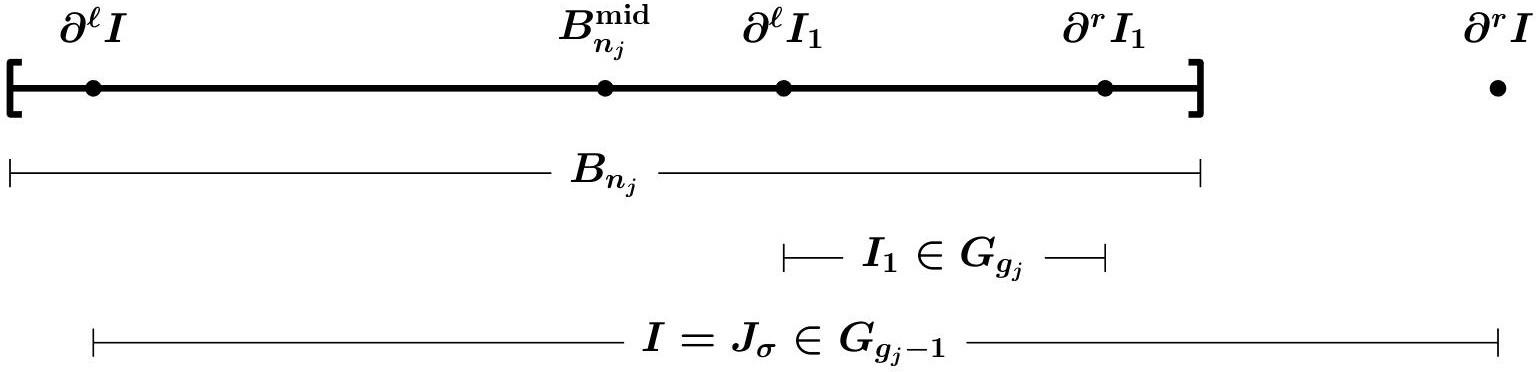
Figure 3. One possibility for Case 1 of the induction step.

We refer the reader to Figure 3. Because $B_{n_{j}}$ is c.w.g. $g_{j}$, $B_{n_{j}}$ contains some basic interval of generation $g_{j}$. Let $I_{1}$ be the rightmost basic interval of generation $g_{j}$ contained in $B_{n_{j}}$, and let $I$ denote the unique basic interval of generation $g_{j}-1$ containing $I_{1}$ by Observation (i). Then $\partial^{\ell}I\leq B_{n_{j}}^{\text{mid}}$. Note that $\partial^{\ell}I$ could be inside or outside $B_{n_{j}}$.

Next, we claim that $\partial^{r}I>\partial^{r}B_{n_{j}}$. To see this, first note that $\partial^{r}I\geq\partial^{\ell}B_{n_{j}}$ because $I_{1}$, and hence $I$, intersects $B_{n_{j}}$. Next we have that $\partial^{r}I\geq\partial^{r}B_{n_{j}}$, for otherwise the interval $\big{(}\partial^{r}I,\partial^{r}B_{n_{j}}\big{)}\subset B_{n_{j}}$ would contain a member of $G_{g_{j}}$ to the right of $I_{1}$ by Observation (vi). Finally, if $\partial^{r}I=\partial^{r}B_{n_{j}}$, then $\partial^{r}B_{n_{j}}\leq\partial^{r}B_{2}<1$ and hence $\partial^{r}I\in\big{.}\big{(}B_{n_{j}}^{\text{mid}},\partial^{r}B_{n_{j}}\big{.}\big{]}$ would be the left endpoint of some basic interval of generation at most $g_{j}-1$. This proves the claim.

Write $I=J_{\sigma}$ for some string $\sigma$ of length $g_{j}-1$. In order to specify Alice’s strategy in choosing $A_{n_{j}}$ we consider two subcases, according as to whether $\partial^{\ell}J_{\sigma 1}\leq\partial^{r}B_{n_{j}}$.

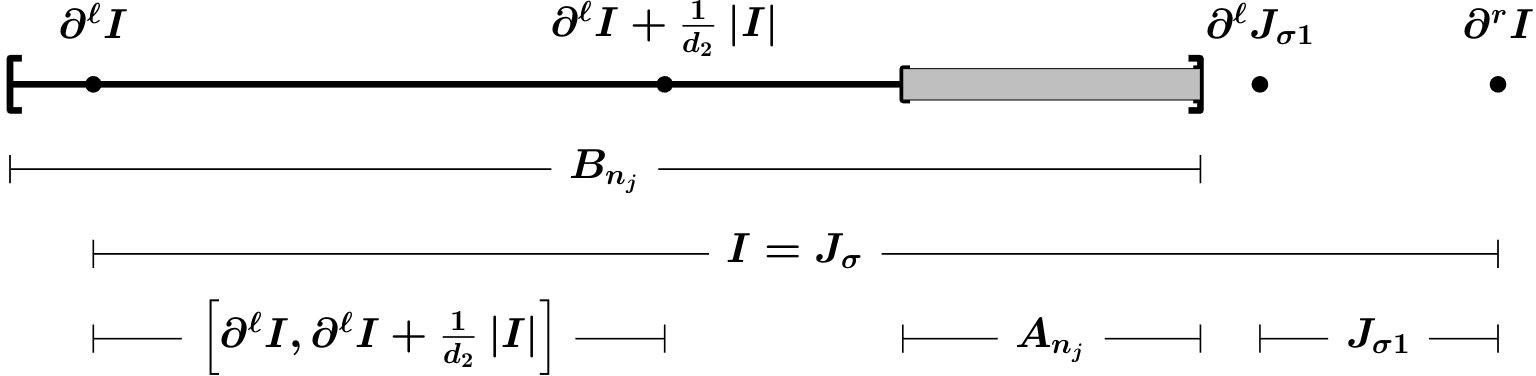
Figure 4. Case 1, Subcase 1 of the induction step.

Subcase 1: $\partial^{\ell}J_{\sigma 1}>\partial^{r}B_{n_{j}}$. See Figure 4. Alice chooses

$$A_{n_{j}}=\left[\partial^{r}B_{n_{j}}-\alpha\left|B_{n_{j}}\right|,\partial^{r}B_{n_{j}}\right]\subset B_{n_{j}}.$$

Using the induction hypothesis $P_{2}\left(j\right)$ we find that

$$\partial^{r}B_{n_{j}}-\left(\partial^{\ell}I+\frac{1}{d_{2}}\left|I\right|\right) \geq\frac{1}{2}\left|B_{n_{j}}\right|-\frac{1}{d_{2}}\left|I\right|>\frac{1}{2}\left|B_{n_{j}}\right|-\frac{d_{1}}{d_{2}}\left|B_{n_{j}}\right|$$

$$>\left(\frac{1}{2}-\frac{d_{1}}{2d_{1}\left(1-2\alpha\right)^{-1}}\right)\left|B_{n_{j}}\right|=\alpha\left|B_{n_{j}}\right|.$$

This shows that $A_{n_{j}}$ is disjoint from $\big{(}\partial^{\ell}I,\partial^{\ell}I+\frac{1}{d_{2}}\left|I\right|\big{)}$. Also $A_{n_{j}}$ is disjoint from $J_{\sigma 1}$ because $\partial^{r}A_{n_{j}}=\partial^{r}B_{n_{j}}<\partial^{\ell}J_{\sigma 1}$. Finally, because $\alpha<\frac{1}{2}$ we have $A_{n_{j}}\subset\big{[}B_{n_{j}}^{\text{mid}},\partial^{r}B_{n_{j}}\big{]}\subset I$ so that $A_{n_{j}}$ is disjoint from every element of $G_{g_{j}-1}\setminus\{I\}$.

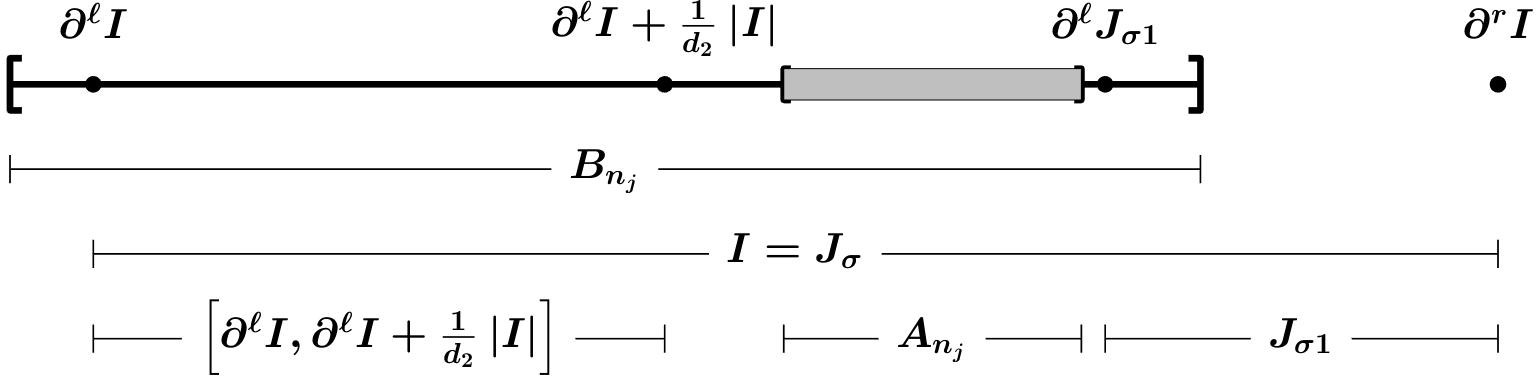
Figure 5. Case 1, Subcase 2 of the induction step.

Subcase 2: $\partial^{\ell}J_{\sigma 1}\leq\partial^{r}B_{n_{j}}$. See Figure 5. In this case $B_{n_{j}}$ must contain $J_{\sigma 2}$ since otherwise $B_{n_{j}}$ would not contain any member of $G_{g_{j}}$. Also $\big{(}\partial^{\ell}I,\partial^{\ell}I+\frac{1}{d_{2}}\left|I\right|\big{)}$ is disjoint from $J_{\sigma 2}$ by Lemma 6.1. Furthermore, by Proposition 4.9,

$$\left|I_{\sigma 2}\right| \geq 2^{-1-\frac{1}{\gamma}}C_{5}^{-1}\left|I\right|>2^{-1-\frac{1}{\gamma}}C_{5}^{-1}\big{|}\big{[}B_{n_{j}}^{\text{mid}},\partial^{r}B_{n_{j}}\big{]}\big{|}$$

$$=2^{-2-\frac{1}{\gamma}}C_{5}^{-1}\left|B_{n_{j}}\right|>\alpha\left|B_{n_{j}}\right|.$$

Thus, as in the previous subcase, Alice may choose $A_{n_{j}}\subset J_{\sigma 2}\subset I$ to be disjoint from $\big{(}\partial^{\ell}I,\partial^{\ell}I+\frac{1}{d_{2}}|I|\big{)}$, $J_{\sigma 1}$, and every element of $G_{g_{j}-1}\setminus\{I\}$.

This takes care of the two subcases. Now Bob chooses $B_{n_{j}+1}$. If $B_{n_{j}+1}$ is c.w.g. $g_{j}$, Alice plays arbitrarily until Bob chooses an interval c.w.g. $g_{j+1}>g_{j}$. This will eventually happen because $A_{n_{j}}$ contains finitely many members of $G_{g_{j}}$ (since $\partial^{\ell}I\notin A_{n_{j}}$) and Alice can force $\left|B_{n}\right|\searrow 0$ by always choosing an interval $A_{n}$ of length $\alpha\left|B_{n}\right|$; hence $B_{n}$ will eventually be too small to contain a member of $G_{g_{j}}$.

Let $n_{j+1}$ be such that $B_{n_{j+1}-1}$ is c.w.g. $g_{j}$ and $B_{n_{j+1}}$ is c.w.g. $g_{j+1}>g_{j}$. Define

$$\mathcal{J}:=\left\{J\in\bigcup_{g=g_{j}}^{g_{j+1}-1}G_{g}\colon J\cap B_{n_{j+1}}\neq\emptyset\right\}.$$

Observe that every $J\in\mathcal{J}$ is contained in $J_{\sigma}$ because $B_{n_{j+1}}$ is disjoint from every element of $G_{g_{j}-1}\setminus\left\{J_{\sigma}\right\}$.

Lemma 6.2.

$\left|B_{n_{j+1}}\right|\geq 2^{-1-\frac{1}{\gamma}}\alpha\beta C_{5}^{-2}\left|J\right|>2^{\frac{1}{\gamma}}C_{5}^{2}d_{2}^{-1}\left|J\right|$ for all $J\in\mathcal{J}$.

Proof.

First observe that every $J\in\mathcal{J}$ is contained in some element of $G_{g_{j}}\cap\mathcal{J}$, and so it suffices to verify the lemma when $J\in G_{g_{j}}\cap\mathcal{J}$. Next, note that the function $n\mapsto\left|J_{\sigma n}\right|$ is strictly decreasing; this follows immediately from the fact that $f^{\prime}$ is increasing. Finally, because $B_{n_{j+1}-1}\subset I$ is c.w.g. $g_{j}$ we may define $k_{0}:=\min\left\{k\colon J_{\sigma k}\subset B_{n_{j+1}-1}\right\}$. Then $k_{0}\geq 2$ by the choice of $A_{n_{j}}$ (or because $\partial^{r}I\notin B_{n_{j}}$ if $B_{n_{j+1}-1}=B_{n_{j}}$). By the definition of $k_{0}$ we have $k_{0}-1=\min\left\{k\colon J_{\sigma k}\cap B_{n_{j+1}-1}\neq\emptyset\right\}\leq\min\left\{k\colon J_{\sigma k}\in\mathcal{J}\right\}$. Using Proposition 4.9 we have

$$\frac{\left|B_{n_{j+1}}\right|}{\max\left\{\left|J\right|\colon J\in G_{g_{j}}\cap\mathcal{J}\right\}} \geq\alpha\beta\frac{\left|B_{n_{j+1}-1}\right|}{\left|J_{\sigma\left(k_{0}-1\right)}\right|}\geq\alpha\beta\frac{\left|J_{\sigma k_{0}}\right|}{\left|J_{\sigma\left(k_{0}-1\right)}\right|}\geq\alpha\beta\frac{C_{5}^{-1}k_{0}^{-1-\frac{1}{\gamma}}}{C_{5}\left(k_{0}-1\right)^{-1-\frac{1}{\gamma}}}$$

$$\geq 2^{-1-\frac{1}{\gamma}}\alpha\beta C_{5}^{-2}=\frac{2^{\frac{1}{\gamma}}C_{5}^{2}}{2^{1+\frac{2}{\gamma}}C_{5}^{4}\left(\alpha\beta\right)^{-1}}>\frac{2^{\frac{1}{\gamma}}C_{5}^{2}}{d_{2}}.\qed$$

Corollary 6.3.

$B_{n_{j+1}}$ is disjoint from every interval $\big{(}\partial^{\ell}J,\partial^{\ell}J+\frac{1}{d_{2}}\left|J\right|\big{)}$, where $J\in\bigcup_{g=0}^{g_{j+1}-2}G_{g}$.

Proof.

$P_{3}\left(j\right)$ is true by the induction hypothesis; therefore it suffices to consider $J\in\bigcup_{g=g_{j}-1}^{g_{j+1}-2}G_{g}$. Also $B_{n_{j+1}}\subset A_{n_{j}}$, $A_{n_{j}}$ is disjoint from $\big{(}\partial^{\ell}I,\partial^{\ell}I+\frac{1}{d_{2}}\left|I\right|\big{)}$, and $I$ is the only element of $G_{g_{j}-1}$ that intersects $\left(A_{n_{j}}\right)^{\circ}$. So it suffices to consider $J\in\bigcup_{g=g_{j}}^{g_{j+1}-2}G_{g}$.

Fix such a $J=J_{\tau}\in G_{g^{\prime}}$, where $g_{j}\leq g^{\prime}\leq g_{j+1}-2$. Using Observation (i) and Corollary 5.6, let $J^{\prime}$ be the unique element of $G_{g^{\prime}}$ containing $B_{n_{j+1}}$. If $J\neq J^{\prime}$, then $B_{n_{j+1}}$ is disjoint from the interior of $J$ and we are done. So suppose $J=J^{\prime}$.

Find the unique $K\in\mathbb{N}$ such that $\partial^{\ell}J+\frac{1}{d_{2}}\left|J\right|\in\left.\left[J_{\tau K}\right.\right)$. By Lemma 6.1, $K-1\geq 2$, and by Corollary 4.10, $K-1\geq\big{(}\frac{C_{5}}{d_{2}}\big{)}^{-\gamma}-2$. So by Proposition 4.9,

$$\frac{\left|\bigcup_{i=K-1}^{\infty}J_{\tau i}\right|}{\left|J\right|} \leq C_{5}\left(K-1\right)^{-\frac{1}{\gamma}}\leq C_{5}\bigg{(}\left(\frac{C_{5}}{d_{2}}\right)^{-\gamma}-2\bigg{)}^{-\frac{1}{\gamma}}$$

$$\leq C_{5}\bigg{(}\frac{1}{2}\left(\frac{C_{5}}{d_{2}}\right)^{-\gamma}\bigg{)}^{-\frac{1}{\gamma}}=\frac{2^{\frac{1}{\gamma}}C_{5}^{2}}{d_{2}}.$$

Therefore, if the left endpoint of $B_{n_{j+1}}$ were contained in $\big{.}\big{[}\partial^{\ell}J,\partial^{\ell}J+\frac{1}{d_{2}}\left|J\right|\big{.}\big{)}$, then $B_{n_{j+1}}$ would contain $J_{\tau\left(K-1\right)}\in G_{g^{\prime}+1}$ by Lemma 6.2. But this is not possible because $B_{n_{j+1}}$ is c.w.g. $g_{j+1}>g^{\prime}+1$. ∎

In conclusion, $P_{1}\left(j+1\right)$ is true by construction, Lemma 6.2 implies $P_{2}\left(j+1\right)$ because $\frac{1}{d_{1}}<2^{-1-\frac{1}{\gamma}}\alpha\beta C_{5}^{-2}$, and Corollary 6.3 is the statement $P_{3}\left(j+1\right)$. This completes the analysis of Case 1.

Case 2: The interval $\bm{\big{.}\big{(}B_{n_{j}}^{\text{mid}},\partial^{r}B_{n_{j}}\big{.}\big{]}}$ contains a left endpoint of generation at most $\bm{g_{j}-1}$

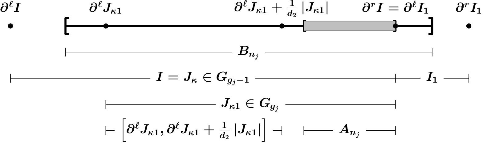
Figure 6. Case 2 of the induction step.

We refer the reader to Figure 6. Let $I_{1}$ be a basic interval of generation at most $g_{j}-1$ with left endpoint in $\big{.}\big{(}B_{n_{j}}^{\text{mid}},\partial^{r}B_{n_{j}}\big{.}\big{]}$. Then there is some basic interval of generation at most $g_{j}-1$ with right endpoint $\partial^{\ell}I_{1}$ by Observation (iv); hence there is some $I=J_{\kappa}\in G_{g_{j}-1}$ having right endpoint $\partial^{\ell}I_{1}$. Note that $\partial^{\ell}I<\partial^{\ell}B_{n_{j}}$ since $\partial^{r}I\in B_{n_{j}}$ and $B_{n_{j}}$ is c.w.g. $g_{j}$. Alice chooses $A_{n_{j}}=\left[\partial^{r}I-\alpha\left|B_{n_{j}}\right|,\partial^{r}I\right]$. Using Proposition 4.9 we have

$$\left|\left[\partial^{\ell}J_{\kappa 1}+\tfrac{1}{d_{2}}\left|J_{\kappa 1}\right|,\partial^{\ell}I\right]\right| \geq C_{5}^{-1}\left|I\right|\left(1-\tfrac{1}{d_{2}}\right)\geq C_{5}^{-1}\big{|}\big{[}\partial^{\ell}B_{n_{j}},B_{n_{j}}^{\text{mid}}\big{]}\big{|}\left(1-\tfrac{1}{d_{2}}\right)$$

$$>\tfrac{1}{4}C_{5}^{-1}\left|B_{n_{j}}\right|>\alpha\left|B_{n_{j}}\right|,$$

which shows that $A_{n_{j}}\subset J_{\kappa 1}$ and moreover, that $A_{n_{j}}$ is disjoint from the interval $\big{[}\partial^{\ell}J_{\kappa 1},\partial^{\ell}J_{\kappa 1}+\frac{1}{d_{2}}\left|J_{\kappa 1}\right|\big{]}$. Thus $A_{n_{j}}$ is disjoint from all intervals $\big{[}\partial^{\ell}J,\partial^{\ell}J+\frac{1}{d_{2}}\left|J\right|\big{]}$ where $J\in G_{g_{j}}$.

Let $A_{n_{j}}$ be c.w.g. $\tilde{g}>g_{j}$. Then by the choice of $A_{n_{j}}$, $J_{\kappa 1\tilde{\kappa}1}\subset A_{n_{j}}\subset J_{\kappa 1\tilde{\kappa}}$, where $\tilde{\kappa}$ is a string of $\tilde{g}-g_{j}-1$ repeating ones. Now Bob chooses $B_{n_{j}+1}$. Define $n_{j+1}:=n_{j}+1$ and let $B_{n_{j+1}}$ be c.w.g. $g_{j+1}\geq\tilde{g}$.

Lemma 6.4.

$\left|B_{n_{j+1}}\right|\geq\beta C_{5}^{-1}\left|J\right|>\tfrac{1}{d_{2}}\left|J\right|$ for all $J\in G_{g_{j+1}-1}$ that intersect $B_{n_{j+1}}$.

Proof.

If $g_{j+1}=\tilde{g}$, then the only basic interval of generation $g_{j+1}-1$ intersecting $B_{n_{j+1}}$ is $J_{\kappa 1\tilde{\kappa}}$, and by Proposition 4.9 we have

$$\left|B_{n_{j+1}}\right|\geq\beta\left|A_{n_{j}}\right|\geq\beta\left|J_{\kappa 1\tilde{\kappa}1}\right|\geq\beta C_{5}^{-1}\left|J_{\kappa 1\tilde{\kappa}}\right|>\tfrac{1}{d_{1}}\left|J_{\kappa 1\tilde{\kappa}}\right|.$$

On the other hand, if $g_{j+1}>\tilde{g}$, then there are at most two basic intervals of generation $g_{j+1}-1$ intersecting $B_{n_{j+1}}$ by Corollaries 5.4 and 5.6. If there is one, call it $J_{\tau t}$; if there are two, call them $J_{\tau t}$ and $J_{\tau(t+1)}$. Both $J_{\tau t}$ and $J_{\tau(t+1)}$ are contained in $J_{\kappa 1\tilde{\kappa}}$. Thus $\left|J_{\tau(t+1)}\right|<\left|J_{\tau t}\right|<\left|J_{\kappa 1\tilde{\kappa}}\right|$ since $f^{\prime}$ is increasing. Borrowing from the calculation above,

$$\left|B_{n_{j+1}}\right| \geq\beta C_{5}^{-1}\left|J_{\kappa 1\tilde{\kappa}}\right|>\beta C_{5}^{-1}\max\left\{\left|J_{\tau(t+1)}\right|,\left|J_{\tau t}\right|\right\}$$

$$>\tfrac{1}{d_{1}}\max\left\{\left|J_{\tau(t+1)}\right|,\left|J_{\tau t}\right|\right\}.\qed$$

Lemma 6.5.

$B_{n_{j+1}}$ is disjoint from every interval $\big{(}\partial^{\ell}J,\partial^{\ell}J+\frac{1}{d_{2}}\left|J\right|\big{)}$, where $J\in\bigcup_{g=0}^{g_{j+1}-2}G_{g}$.

Proof.

We use the same notation as in the previous lemma. $P_{3}\left(j\right)$ is true by the induction hypothesis; therefore it suffices to consider $J\in\bigcup_{g=g_{j}-1}^{g_{j+1}-2}G_{g}$. Also $B_{n_{j+1}}\subset A_{n_{j}}\subset J_{\kappa 1}$, $J_{\kappa 1}$ is disjoint from $\big{(}\partial^{\ell}I,\partial^{\ell}I+\frac{1}{d_{2}}\left|I\right|\big{)}$ by Lemma 6.1, and $I$ is the only element of $G_{g_{j}-1}$ that intersects $\left(A_{n_{j}}\right)^{\circ}$. So it suffices to consider $J\in\bigcup_{g=g_{j}}^{g_{j+1}-2}G_{g}$.

Fix such a $J\in G_{g}$, where $g_{j}\leq g\leq g_{j+1}-2$. Let $J^{\prime}$ be the unique element of $G_{g}$ containing $J_{\tau(t+1)}$ and $J_{\tau t}$. If $J\neq J^{\prime}$, then $B_{n_{j+1}}$ is disjoint from the interior of $J$ and we are done. So suppose $J=J^{\prime}$. Thus $J=J_{\kappa 1\kappa^{\prime}}$ where $\kappa^{\prime}$ is a string of $g-g_{j}$ repeating ones. We consider two cases, the first of which (Case A) is potentially vacuous.

Case A: $g_{j}\leq g\leq\tilde{g}-2$. Recall that $B_{n_{j+1}}\subset A_{n_{j}}\subset J_{\kappa 1\tilde{\kappa}}\in G_{\tilde{g}-1}$ where $\tilde{\kappa}$ is a string of $\tilde{g}-g_{j}-1$ repeating ones. Also $J=J_{\kappa 1\kappa^{\prime}}$ where $\kappa^{\prime}$ is a string of $g-g_{j}$ repeating ones; but $\left|\kappa^{\prime}\right|=g-g_{j}\leq\tilde{g}-g_{j}-2<\tilde{g}-g_{j}-1=\left|\tilde{\kappa}\right|$, and $\big{(}\partial^{\ell}J,\partial^{\ell}J+\frac{1}{d_{2}}\left|J\right|\big{)}\subset\bigcup_{i=3}^{\infty}J_{\kappa 1\kappa^{\prime}i}$ by Lemma 6.1. The result follows in this case.

Case B: $\tilde{g}-1\leq g\leq g_{j+1}-2$. Find the unique $K$ such that $\partial^{\ell}J+\frac{1}{d_{2}}\left|J\right|\in\left.\left[J_{\kappa 1\kappa^{\prime}K}\right.\right)$. By Lemma 6.1, $K-1\geq 2$, and by Corollary 4.10, $K-1\geq\big{(}\frac{C_{5}}{d_{2}}\big{)}^{-\gamma}-2$. Thus, using Proposition 4.9,

$$\frac{\left|\bigcup_{i=K-1}^{\infty}J_{\kappa 1\kappa^{\prime}i}\right|}{\left|J\right|} \leq C_{5}\left(K-1\right)^{-\frac{1}{\gamma}}\leq C_{5}\bigg{(}\left(\frac{C_{5}}{d_{2}}\right)^{-\gamma}-2\bigg{)}^{-\frac{1}{\gamma}}$$

$$\leq C_{5}\bigg{(}\frac{1}{2}\left(\frac{C_{5}}{d_{2}}\right)^{-\gamma}\bigg{)}^{-\frac{1}{\gamma}}=\frac{2^{\frac{1}{\gamma}}C_{5}^{2}}{d_{2}}.$$

Also $\left|\kappa^{\prime}\right|=g-g_{j}\geq\tilde{g}-g_{j}-1=\left|\tilde{\kappa}\right|$ and so by Proposition 4.9,

$$\frac{\left|B_{n_{j+1}}\right|}{\left|J\right|}\geq\beta\frac{\left|A_{n_{j}}\right|}{\left|J\right|}\geq\beta\frac{\left|J_{\kappa 1\tilde{\kappa}1}\right|}{\left|J_{\kappa 1\kappa^{\prime}}\right|}\geq\beta\frac{\left|J_{\kappa 1\tilde{\kappa}1}\right|}{\left|J_{\kappa 1\tilde{\kappa}}\right|}\geq\beta C_{5}^{-1}>\frac{2^{\frac{1}{\gamma}}C_{5}^{2}}{d_{2}}.$$

Therefore, if the left endpoint of $B_{n_{j+1}}$ were contained in $\big{.}\big{[}\partial^{\ell}J,\partial^{\ell}J+\frac{1}{d_{2}}\left|J\right|\big{.}\big{)}$, then $B_{n_{j+1}}$ would contain $J_{\kappa 1\kappa^{\prime}\left(K-1\right)}\in G_{g+1}$. But this is not possible because $B_{n_{j+1}}$ is c.w.g. $g_{j+1}>g+1$. ∎

In conclusion, $P_{1}\left(j+1\right)$ is true by construction, Lemma 6.4 is the statement $P_{2}\left(j+1\right)$, and Lemma 6.5 is the statement $P_{3}\left(j+1\right)$. This completes the analysis of Case 2. The induction argument is complete, and with it, the proof of Theorem 2.1.

7. Proof that $\mathcal{E}_{f}$ is strong winning (Theorem 1.1)

Let $\mathcal{E}_{F}$ be $\alpha_{F}$-strong winning (with $\alpha_{F}\leq\frac{1}{2}$) and define $\alpha_{f}:=\exp\left(-C_{2}\right)\alpha_{F}$ (the constant $C_{2}$ is defined in Theorem 4.4). Let $\beta_{f}\in\left(0,\exp\left(-C_{2}\right)\right)$ be arbitrary and define $\beta_{F}:=\exp\left(C_{2}\right)\beta_{f}$. We claim that $\mathcal{E}_{f}$ is $\left(\alpha_{f},\beta_{f}\right)$-strong winning. In order to prove this we set up two $\left(\alpha,\beta\right)$ games; Alice and Bob will play the primary $\left(\alpha_{f},\beta_{f}\right)$ game on $\left(\left[0,1\right],\mathcal{E}_{f}\right)$, and Alicia and Bobby will play an auxiliary $\left(\alpha_{F},\beta_{F}\right)$ game on $\left(\left[r_{1},1\right],\mathcal{E}_{F}\right)$.

The main game begins as Bob chooses $B_{1}\subset\left[0,1\right]$. Alice chooses $A_{1}$ such that $0\notin A_{1}$. Bob chooses $B_{2}$. Alice plays arbitrarily until Bob chooses an interval that is contained in some $\left[r_{n+1},r_{n}\right]$. This will eventually happen for the following reason. There are finitely many intervals $\left[r_{n+1},r_{n}\right]$ that intersect $B_{2}$ (because $0\notin B_{2}$), and Alice can force $\left|B_{n}\right|\searrow 0$ by always choosing an interval $A_{n}$ of length $\alpha_{f}\left|B_{n}\right|$. Furthermore $\alpha_{f}<\frac{1}{2}$ and so Alice may always choose $A_{n}$ so as to avoid any given point in $B_{n}$. After relabeling we may therefore assume without loss of generality that $B_{1}\subset\left[r_{n+1},r_{n}\right]$ for some $n\in\mathbb{N}$.

The auxiliary game begins as Bobby chooses $B_{1}^{\prime}=f^{n}\left(B_{1}\right)\subset\left[r_{1},1\right]$. Alicia, as part of her winning strategy, chooses $A_{1}^{\prime}\subset B_{1}^{\prime}$. Define $A_{1}=f^{-n}\left(A_{1}^{\prime}\right)\cap\left[r_{n+1},r_{n}\right]\subset B_{1}$. By the Mean Value Theorem there exist $\xi,\xi^{\prime}\in B_{1}$ such that

$$\frac{\left|A_{1}\right|}{\left|B_{1}\right|}=\frac{\left|A_{1}^{\prime}\right|/\left(f^{n}\right)^{\prime}\left(\xi\right)}{\left|B_{1}^{\prime}\right|/\left(f^{n}\right)^{\prime}\left(\xi^{\prime}\right)}\geq\exp\left(-\frac{C_{2}}{r_{0}-r_{1}}\left|f^{n}\xi-f^{n}\xi^{\prime}\right|\right)\alpha_{F}\geq\alpha_{f}.$$

Thus $A_{1}$ is a permissible interval for Alice to choose; she does so.

Suppose the four players have chosen intervals $\left\{A_{i},B_{i},A_{i}^{\prime},B_{i}^{\prime}\right\}_{i=1}^{k}$ for some $k\in\mathbb{N}$ in such a way that $f^{n}\left(B_{k}\right)=B_{k}^{\prime}$ and $A_{k}=f^{-n}\left(A_{k}^{\prime}\right)\cap\left[r_{n+1},r_{n}\right]$, and $A_{k}$ is chosen as part of Alicia’s winning strategy. Bob chooses $B_{k+1}\subset A_{k}$. Define $B_{k+1}^{\prime}=f^{n}\left(B_{k+1}\right)\subset A_{k}^{\prime}$. By the Mean Value Theorem there exist $\eta,\eta^{\prime}\in A_{k}$ such that

$$\frac{\left|B_{k+1}^{\prime}\right|}{\left|A_{k}^{\prime}\right|}=\frac{\left|B_{k+1}\right|}{\left|A_{k}\right|}\frac{\left(f^{n}\right)^{\prime}\left(\eta\right)}{\left(f^{n}\right)^{\prime}\left(\eta^{\prime}\right)}\geq\exp\left(-\frac{C_{2}}{r_{0}-r_{1}}\left|f^{n}\eta-f^{n}\eta^{\prime}\right|\right)\beta_{f}\geq\beta_{F}.$$

Thus $B_{k+1}^{\prime}$ is a permissible interval for Bobby to choose; he does so. Alicia, as part of her winning strategy, chooses $A_{k+1}^{\prime}\subset B_{k+1}^{\prime}$. Define $A_{k+1}=f^{-n}\left(A_{k+1}^{\prime}\right)\cap\left[r_{n+1},r_{n}\right]\subset B_{k+1}$. By the Mean Value Theorem there exist $\upsilon,\upsilon^{\prime}\in B_{k+1}$ such that

$$\frac{\left|A_{k+1}\right|}{\left|B_{k+1}\right|}=\frac{\left|A_{k+1}^{\prime}\right|/\left(f^{n}\right)^{\prime}\left(\upsilon\right)}{\left|B_{k+1}^{\prime}\right|/\left(f^{n}\right)^{\prime}\left(\upsilon^{\prime}\right)}\geq\exp\left(-\frac{C_{2}}{r_{0}-r_{1}}\left|f^{n}\upsilon-f^{n}\upsilon^{\prime}\right|\right)\alpha_{F}\geq\alpha_{f}.$$

Thus $A_{k+1}$ is a permissible interval for Alicia to choose; she does so.

This completes the induction. Define $\{\omega\}=\bigcap_{k=1}^{\infty}B_{k}$ and $\{\omega^{\prime}\}=\bigcap_{k=1}^{\infty}B_{k}^{\prime}$. By construction, Alicia wins; thus there exists $L\in\mathbb{N}$ such that the orbit of $\omega^{\prime}$ under $F$ stays outside the interval $\left.\left[r_{1},p_{L}\right.\right)$. Define $M:=2+\max\left\{L,n\right\}$. We claim that the orbit of $\omega$ under $f$ stays outside the interval $\left.\left[0,r_{M}\right.\right)$.

Suppose otherwise. Write $\omega^{\prime}\in J_{m_{1}m_{2}\dots}$ and let

$$\tau:=\min\left\{t\in\mathbb{N}\cup\{0\}\colon f^{t}\omega\in\left.\left[0,r_{M}\right.\right)\right\}.$$

Because $M>n+1$ and $\omega\in\left[r_{n+1},r_{n}\right]$ we have $\tau>n$. Find $j\geq 0$ and $0\leq s<m_{j+1}$ such that

$$\tau=n+m_{1}+\dots+m_{j}+s.$$

Because the orbit of $\omega^{\prime}$ under $F$ avoids $\left.\left[r_{1},p_{L}\right.\right)$ we have that $m_{i}\leq L<M$ for all $i$. Therefore

$$F^{j+1}\omega^{\prime}=f^{m_{1}+\dots m_{j+1}+n}\omega=f^{m_{j+1}-s}\left(f^{\tau}\omega\right)\in\left.\left[0,r_{M-m_{j+1}+s}\right.\right)\subset\left.\left[0,r_{1}\right.\right).$$

But $F^{j+1}\omega^{\prime}\in J_{m_{j+2}}\subset\left[r_{1},1\right]$, a contradiction.

This shows that $\mathcal{E}_{f}$ is $\left(\alpha_{f},\beta_{f}\right)$-strong winning whenever $\beta_{f}\in\left(0,\exp\left(-C_{2}\right)\right)$. Clearly this implies that $\mathcal{E}_{f}$ is $\left(\alpha_{f},\beta\right)$-strong winning for all $\beta\in\left(0,1\right)$. Hence $\mathcal{E}_{f}$ is $\alpha_{f}$-strong winning.

8. Acknowledgments

The author would like to thank his Ph.D. advisor, Vaughn Climenhaga, for his infinite patience and wisdom.

References

- [1] R. Broderick, L. Fishman, and D. Kleinbock, “Schmidt’s game, fractals, and orbits of toral endomorphisms,” Ergodic Theory Dynam. Systems, vol. 31, no. 4, pp. 1095–1107, 2011.
- [2] S. G. Dani, “On orbits of endomorphisms of tori and the Schmidt game,” Ergodic Theory Dynam. Systems, vol. 8, no. 4, pp. 523–529, 1988.
- [3] D. Färm, T. Persson, and J. Schmeling, “Dimension of countable intersections of some sets arising in expansions in non-integer bases,” Fund. Math., vol. 209, no. 2, pp. 157–176, 2010.
- [4] H. Hu and Y. Yu, “On Schmidt’s game and the set of points with non-dense orbits under a class of expanding maps,” J. Math. Anal. Appl., vol. 418, no. 2, pp. 906–920, 2014.
- [5] W. M. Schmidt, “On badly approximable numbers and certain games,” Trans. Amer. Math. Soc., vol. 123, pp. 178–199, 1966.
- [6] J. Tseng, “Schmidt games and Markov partitions,” Nonlinearity, vol. 22, no. 3, pp. 525–543, 2009.
- [7] K. Gelfert and M. Rams, “The Lyapunov spectrum of some parabolic systems,” Ergodic Theory Dynam. Systems, vol. 29, no. 3, pp. 919–940, 2009.
- [8] K. Nakaishi, “Multifractal formalism for some parabolic maps,” Ergodic Theory Dynam. Systems, vol. 20, no. 3, pp. 843–857, 2000.
- [9] M. Thaler, “Estimates of the invariant densities of endomorphisms with indifferent fixed points,” Israel J. Math., vol. 37, no. 4, pp. 303–314, 1980.
- [10] B. Mance and J. Tseng, “Bounded Lüroth expansions: applying Schmidt games where infinite distortion exists,” Acta Arith., vol. 158, no. 1, pp. 33–47, 2013.
- [11] C. T. McMullen, “Winning sets, quasiconformal maps and Diophantine approximation,” Geom. Funct. Anal., vol. 20, no. 3, pp. 726–740, 2010.
- [12] L.-S. Young, “Recurrence times and rates of mixing,” Israel J. Math., vol. 110, pp. 153–188, 1999.