Reviewing and Improving the Gaussian Mechanism for Differential Privacy

Abstract

Differential privacy provides a rigorous framework to quantify data privacy, and has received considerable interest recently. A randomized mechanism satisfying $(\epsilon,\delta)$-differential privacy (DP) roughly means that, except with a small probability $\delta$, altering a record in a dataset cannot change the probability that an output is seen by more than a multiplicative factor $e^{\epsilon}$. A well-known solution to $(\epsilon,\delta)$-DP is the Gaussian mechanism initiated by Dwork et al. [1] in 2006 with an improvement by Dwork and Roth [2] in 2014, where a Gaussian noise amount $\sqrt{2\ln\frac{2}{\delta}}\times\frac{\Delta}{\epsilon}$ of [1] or $\sqrt{2\ln\frac{1.25}{\delta}}\times\frac{\Delta}{\epsilon}$ of [2] is added independently to each dimension of the query result, for a query with $\ell_{2}$-sensitivity $\Delta$. Although both classical Gaussian mechanisms [1, 2] explicitly assume $0<\epsilon\leq 1$ only, our review finds that many studies in the literature have used the classical Gaussian mechanisms under values of $\epsilon$ and $\delta$ where we show the added noise amounts of [1, 2] do not achieve $(\epsilon,\delta)$-DP. We obtain such result by analyzing the optimal (i.e., least) Gaussian noise amount $\sigma_{\texttt{DP-OPT}}$ for $(\epsilon,\delta)$-DP and identifying the set of $\epsilon$ and $\delta$ where the noise amounts of classical Gaussian mechanisms are even less than $\sigma_{\texttt{DP-OPT}}$. The inapplicability of mechanisms of [1, 2] to large $\epsilon$ can also be seen from our result that $\sigma_{\texttt{DP-OPT}}$ for large $\epsilon$ can be written as $\Theta\big{(}\frac{1}{\sqrt{\epsilon}}\big{)}$, but not $\Theta\left(\frac{1}{\epsilon}\right)$.

Since $\sigma_{\texttt{DP-OPT}}$ has no closed-form expression and needs to be approximated in an iterative manner, we propose Gaussian mechanisms by deriving closed-form upper bounds for $\sigma_{\texttt{DP-OPT}}$. Our mechanisms achieve $(\epsilon,\delta)$-DP for any $\epsilon$, while the classical Gaussian mechanisms [1, 2] do not achieve $(\epsilon,\delta)$-DP for large $\epsilon$ given $\delta$. Moreover, the utilities of our proposed Gaussian mechanisms improve those of the classical Gaussian mechanisms [1, 2] and are close to that of the optimal yet more computationally expensive Gaussian mechanism.

Since most mechanisms proposed in the literature for $(\epsilon,\delta)$-DP are obtained by ensuring a condition called $(\epsilon,\delta)$-probabilistic differential privacy (pDP), we also present an extensive discussion of $(\epsilon,\delta)$-pDP including deriving Gaussian noise amounts to achieve it.

To summarize, our paper fixes the literature’s long-time misuse of Gaussian mechanism [1, 2] for $(\epsilon,\delta)$-differential privacy and provides a comprehensive study for the Gaussian mechanisms.

I Introduction

Differential privacy. Differential privacy [3] has received considerable interest [1, 4, 5, 6, 7, 8, 9, 10, 11] since it provides a rigorous framework to quantify data privacy. Roughly speaking, a randomized mechanism achieving $(\epsilon,\delta)$-differential privacy (DP) means that, except with a (typically small) probability $\delta$, altering a record in a dataset cannot change the probability that an output is seen by more than a multiplicative factor $e^{\epsilon}$. Formally, for $D$ and $D^{\prime}$ iterating through all pairs of neighboring datasets which differ by one record, and for $\mathcal{Y}$ iterating through all subsets of the output range of a randomized mechanism $Y$, the mechanism $Y$ achieves $(\epsilon,\delta)$-DP if ${\mathbb{P}}\left[{Y(D)\in\mathcal{Y}}\right]\leq e^{\epsilon}{\mathbb{P}}\left[{Y(D^{\prime})\in\mathcal{Y}}\right]+\delta,$ where ${\mathbb{P}}\left[{\cdot}\right]$ denotes the probability, and the probability space is over the coin flips of the randomized mechanism $Y$. If $\delta=0$, the notion of $(\epsilon,\delta)$-DP becomes $\epsilon$-DP.

Classical Gaussian mechanisms [1, 2] to achieve $(\epsilon,\delta)$-differential privacy. Among various mechanisms to achieve DP, the Gaussian mechanism for real-valued queries initiated by [1] has received much attention, where a certain amount of zero-mean Gaussian noise is added independently to each dimension of the query result. Below, for a Gaussian mechanism with parameter $\sigma$, we mean that $\sigma$ is the standard deviation of the Gaussian noise.

As shown in [1, 2], the noise amount in the Gaussian mechanism scales with the $\ell_{2}$-sensitivity $\Delta$ of a query, which is defined as the maximal $\ell_{2}$ distance between the true query results for any two neighboring datasets $D$ and $D^{\prime}$ that differ in one record; i.e., $\Delta=\max_{\textrm{neighboring $D,D^{\prime}$}}\|Q(D)-Q(D^{\prime})\|_{2}$. We will elaborate the notion of neighboring datasets in Remark 1 on Page 1. For a query with $\ell_{2}$-sensitivity $\Delta$, the noise amount in the first Gaussian mechanism proposed by Dwork et al. [1] in 2006 to achieve $(\epsilon,\delta)$-DP, denoted by Dwork-2006, is given by

$$\textstyle{\sigma_{\texttt{Dwork-2006}}:=\sqrt{2\ln\frac{2}{\delta}}\times\frac{\Delta}{\epsilon}.}$$ (1)

Improving Dwork-2006 via a smaller amount of noise addition, the Gaussian mechanism by Dwork and Roth [2] in 2014, denoted by Dwork-2014, adds Gaussian noise with standard deviation

$$\textstyle{\sigma_{\texttt{Dwork-2014}}:=\sqrt{2\ln\frac{1.25}{\delta}}\times\frac{\Delta}{\epsilon}.}$$ (2)

Both Page 6 in [1] for Dwork-2006 and Theorem A.1 on Page 261 in [2] for Dwork-2014 consider $\epsilon\leq 1$. We will formally prove that Dwork-2006 and Dwork-2014 fail to achieve $(\epsilon,\delta)$-DP for large $\epsilon$ given $\delta$. Moreover, we will show in Section III that many studies [12, 13, 14, 15, 16, 17, 7, 8, 18, 19, 20, 21] applying Dwork-2006 and Dwork-2014 neglect the condition $\epsilon\leq 1$, and use Dwork-2006 or Dwork-2014 under values of $\epsilon$ and $\delta$ where the added Gaussian noise amount actually does not achieve $(\epsilon,\delta)$-DP. This renders their obtained results inaccurate.

One may wonder why we consider both mechanisms since clearly it holds that

$$\text{$\sigma_{\texttt{Dwork-2014}}$ in Eq.~{}(\ref{dwork-2014})}<\text{$\sigma_{\texttt{Dwork-2006}}$ in Eq.~{}(\ref{dwork-2006})}.$$ (3)

The reason is as follows. Although Dwork-2014 achieves higher utility than that of Dwork-2006 for the set of $\epsilon$ and $\delta$ under which they both achieve $(\epsilon,\delta)$-DP, Dwork-2006 has wider applicability than Dwork-2014; i.e., the set of $\epsilon$ and $\delta$ where Dwork-2014 achieves $(\epsilon,\delta)$-DP is a strict subset of the set of $\epsilon$ and $\delta$ where Dwork-2006 achieves $(\epsilon,\delta)$-DP. Given the above, we discuss both mechanisms.

Our contributions. We make the following contributions in this paper.

1. Failures of classical Gaussian mechanisms for large $\epsilon$. We prove (in Theorem 1 on Page 1) that the classical Gaussian mechanisms Dwork-2006 of [1] and Dwork-2014 of [2] fail to achieve $(\epsilon,\delta)$-DP for large $\epsilon$ given $\delta$. In fact, we prove that for any Gaussian mechanism with noise amount $F(\delta)\times\frac{\Delta}{\epsilon}$ for some function $F(\delta)$, there exists a positive function $G(\delta)$ for any $0<\delta<1$ such that the above Gaussian mechanism does not achieve $(\epsilon,\delta)$-DP for any $\epsilon>G(\delta)$. The above result applies to Dwork-2006 and Dwork-2014, where the former specifies $F(\delta)$ as $\sqrt{2\ln\frac{2}{\delta}}$ and the latter specifies $F(\delta)$ as $\sqrt{2\ln\frac{1.25}{\delta}}$.

2. The literature’s misuse of classical Gaussian mechanisms for large $\epsilon$. After a literature review (in Table I on Page I), we find that many papers [12, 13, 14, 15, 16, 17, 7, 8, 18, 19, 20, 21] use the classical Gaussian mechanism Dwork-2006 or Dwork-2014 under values of $\epsilon$ and $\delta$ where the added noise amount actually does not achieve $(\epsilon,\delta)$-DP. This makes their obtained results inaccurate.

3. An $\epsilon$-independent upper bound and asympotics of the optimal Gaussian noise amount for $(\epsilon,\delta)$-DP. We prove (in Theorem 3 on Page 3) that the optimal (i.e., least) Gaussian noise amount $\sigma_{\texttt{DP-OPT}}$ for $(\epsilon,\delta)$-DP is always less than $\frac{\Delta}{2\sqrt{2}\cdot\operatorname*{inverf}(\delta)}$, which does not depend on $\epsilon$, where $\operatorname*{inverf}()$ denotes the inverse of the error function. This is in contrast to the classical Gaussian mechanisms’ noise amounts $\sigma_{\texttt{Dwork-2006}}$ in Eq. (1) and $\sigma_{\texttt{Dwork-2014}}$ in Eq. (2) which scale with $\frac{1}{\epsilon}$ and tend to $\infty$ as $\epsilon\to 0$. In fact, we prove that $\sigma_{\texttt{DP-OPT}}$ given a fixed $\delta$ converges to its upper bound $\frac{\Delta}{2\sqrt{2}\cdot\operatorname*{inverf}(\delta)}$ as $\epsilon\to 0$, and is $\Theta\left(\frac{1}{\sqrt{\epsilon}}\right)$ as $\epsilon\to\infty$. Also, we show that $\sigma_{\texttt{DP-OPT}}$ given a fixed $\epsilon$ is $\Theta\left(\sqrt{\ln\frac{1}{\delta}}\hskip 1.5pt\right)$ as $\delta\to 0$.

4. Our Gaussian mechanisms for $(\epsilon,\delta)$-differential privacy with closed-form expressions. Although the optimal Gaussian mechanism for $(\epsilon,\delta)$-DP has been proposed in a very recent work [22], its noise amount $\sigma_{\texttt{DP-OPT}}$ has no closed-form expression and needs to be approximated in an iterative manner. Hence, we propose new Gaussian mechanisms (Mechanism 1 and Mechanism 2 in Theorems 4 and 5 on Page 4) by deriving closed-form upper bounds for $\sigma_{\texttt{DP-OPT}}$. We summarize the advantages of our Gaussian mechanisms as follows.

   • As discussed, our Gaussian mechanisms have closed-form expressions and are computationally efficient than [22]’s optimal Gaussian noise amount, which has no closed-form expression and needs to be approximated in an iterative manner. In addition, both numerical and experimental studies show that the utilities of our Gaussian mechanisms are close to that of the optimal yet more computationally expensive Gaussian mechanism by [22].

   • Our Gaussian mechanisms all achieve $(\epsilon,\delta)$-DP for any $\epsilon$, while the classical Gaussian mechanisms Dwork-2006 of [1] and Dwork-2014 of [2] were proposed for only $0<\epsilon\leq 1$ and we show that they do not achieve $(\epsilon,\delta)$-DP for large $\epsilon$ given $\delta$, as noted in Contribution 1) above.

   • We prove (in Inequality (10) on Page 10) that the noise amounts of our Gaussian mechanisms are less than that of Dwork-2014 (and hence also less than that of Dwork-2006), for $0<\epsilon\leq 1$ where the proofs of Dwork-2006 of [1] and Dwork-2014 of [2] require.

   • For a subset of $\epsilon>1$ where Dwork-2014 happens to work (Dwork-2014’s original proof requires $\epsilon\leq 1$), experiments (in Figure 2 on Page 2) show that our Mechanism 1 often adds noise amount less than that of Dwork-2014.

5. $(\epsilon,\delta)$-Differential privacy versus $(\epsilon,\delta)$-probabilistic differential privacy. Since most mechanisms proposed in the literature for $(\epsilon,\delta)$-differential privacy (DP) are obtained by ensuring a notion called $(\epsilon,\delta)$-probabilistic differential privacy (pDP), which requires the privacy loss random variable to fall in the interval $[-\epsilon,\epsilon]$ with probability at least $1-\delta$, we also investigate $(\epsilon,\delta)$-pDP, and show its difference/relationship with $(\epsilon,\delta)$-DP (in Section VI on Page VI). In particular, the minimal Gaussian noise amount to achieve $(\epsilon,\delta)$-pDP given $\delta$ scales with $\frac{1}{\epsilon}$ as $\epsilon\to 0$ (from Theorem 7 on Page 7), while the minimal Gaussian noise amount to achieve $(\epsilon,\delta)$-DP given $\delta$ converges to its upper bound $\frac{\Delta}{2\sqrt{2}\cdot\operatorname*{inverf}(\delta)}$ as $\epsilon\to 0$ (from Theorem 3 on Page 3). Moreover, while clearly $(\epsilon,\delta)$-pDP implies $(\epsilon,\delta)$-DP, we also prove that $(\epsilon,\delta)$-DP implies $(\epsilon_{*},\frac{\delta(1+e^{-\epsilon_{*}})}{1-e^{\epsilon-\epsilon_{*}}})$-pDP for any $\epsilon_{*}>\epsilon$.

6. Gaussian mechanisms for $(\epsilon,\delta)$-probabilistic differential privacy. For $(\epsilon,\delta)$-pDP, we also derive the optimal Gaussian mechanism (in Theorem 6 on Page 6) which adds the least amount of Gaussian noise (denoted by $\sigma_{\texttt{pDP-OPT}}$). However, since $\sigma_{\texttt{pDP-OPT}}$ has no closed-form expression and needs to be approximated in an iterative manner, we propose Gaussian mechanisms for $(\epsilon,\delta)$-pDP (Mechanism 3 and Mechanism 4 in Theorems 8 and 9 on Page 8) by deriving more computationally efficient upper bounds (in closed-form expressions) for $\sigma_{\texttt{pDP-OPT}}$.

Organization. The rest of the paper is organized as follows.

• Section II surveys related work.

• In Section III, we elaborate $(\epsilon,\delta)$-differential privacy (DP) and review the literature’s misuse of classical Gaussian mechanisms.

• In Section IV, we discuss the optimal Gaussian mechanism for $(\epsilon,\delta)$-DP, where the noise amount has no closed-form expression.

• Section V presents our Gaussian mechanisms for $(\epsilon,\delta)$-DP with closed-form expressions of noise amounts.

• Since most mechanisms proposed in the literature for $(\epsilon,\delta)$-DP are obtained by ensuring a notion called $(\epsilon,\delta)$-probabilistic differential privacy (pDP), Section VI is devoted to $(\epsilon,\delta)$-pDP, where we discuss the difference/relationship between $(\epsilon,\delta)$-pDP and $(\epsilon,\delta)$-DP, and derive the optimal Gaussian mechanism for $(\epsilon,\delta)$-pDP, where the noise amount has no closed-form expression. Then we propose Gaussian mechanisms for $(\epsilon,\delta)$-pDP with closed-form expressions of noise amounts.

• In view that concentrated differential privacy [9] and related notions [10, 23, 24] have recently been proposed as variants of differential privacy, we show in Section VII that achieving $(\epsilon,\delta)$-DP by ensuring one of these privacy definitions gives Gaussian mechanisms worse than ours.

• Section VIII presents experimental results.

• We conclude the paper in Section IX.

Due to the space limitation, additional details including the proofs are provided in the appendices of this supplementary file.

Notation. Throughout the paper, ${\mathbb{P}}\left[{\cdot}\right]$ denotes the probability, and ${\mathbb{F}}\left[{\cdot}\right]$ stands for the probability density function. The error function is denoted by ${\operatorname*{erf}}()$, and its complement is ${\operatorname*{erfc}}()$; i.e., ${\operatorname*{erf}}(x):=\frac{2}{\sqrt{\pi}}\int_{0}^{x}e^{-{t}^{2}}\hskip 1.0pt\emph{d}t$ and ${\operatorname*{erfc}}(x):=1-{\operatorname*{erf}}(x)$. In addition, $\operatorname*{inverf}()$ is the inverse of the error function, and $\operatorname*{inverfc}()$ is the inverse of the complementary error function.

II Related Work

Differential privacy. The notion of differential privacy (DP) [3] has received much attention [25, 26, 27, 28, 29, 30] since it provides a rigorous framework to quantify data privacy. The Gaussian mechanism to achieve DP has been investigated in [1, 2], while the Laplace mechanism is introduced in [3] and the exponential mechanism is proposed in [31]. The Gaussian (resp., Laplace) mechanism adds independent Gaussian (resp., Laplace) noise to each dimension of the query result, while the exponential mechanism can address non-numeric queries. Recently, the following mechanisms to achieve DP have been proposed: the truncated Laplacian mechanism [32], the staircase mechanism [33, 34], and the Podium mechanism [35]. Compared with these mechanisms, the Gaussian mechanism is more friendly for composition analysis since the privacy loss random variable (defined in Section VI on Page VI) after composing independent Gaussian mechanisms follows a Gaussian distribution, whereas the privacy loss after composing independent truncated Laplacian mechanisms (staircase mechanisms, or podium mechanisms) has a complicated probability distribution.

Use of Gaussian mechanism. The Gaussian mechanism has been used by Dwork et al. [27] to design algorithms for privacy-preserving principal component analysis. Nikolov et al. [28] leverage the Gaussian mechanism for differentially private release of a $k$-way marginal query. The Gaussian mechanism is also used by Hsu et al. [29] for enabling multiple parties to distributedly solve convex optimization problems in a privacy-preserving and distributed manner. Gilbert and McMillan  [36] apply the Gaussian mechanism to differentially private recovery of heat source location. Bun et al. [37] employ the Gaussian mechanism to derive a lower bound on the length of a combinatorial object called a fingerprinting code, proposed by Boneh and Shaw [38] for watermarking copyrighted content. Abadi et al. [26] apply $(\epsilon,\delta)$-DP to stochastic gradient descent of deep learning, where the Gaussian mechanism is used for adding noise to the gradient. Recently, Liu [39] have presented a generalized Gaussian mechanism based on the $\ell_{p}$-sensitivity${}^{\text{\ref{footnotelp}}}$.

Probabilistic differential privacy. Most mechanisms proposed in the literature for $(\epsilon,\delta)$-DP are obtained by ensuring a notion called $(\epsilon,\delta)$-probabilistic differential privacy (pDP) [40], which requires the privacy loss random variable to fall in the interval $[-\epsilon,\epsilon]$ with probability at least $1-\delta$. For the formal definition and results discussed below, see Section VI for details, where we present i) relations between $(\epsilon,\delta)$-DP and $(\epsilon,\delta)$-pDP, ii) an analytical but not closed-form expression for the optimal Gaussian mechanism (denoted by Mechanism pDP-OPT) to achieve $(\epsilon,\delta)$-pDP, and iii) Gaussian mechanisms for $(\epsilon,\delta)$-pDP, denoted by Mechanism 3 and Mechanism 4, respectively.

Other variants of differential privacy. Different variants of differential privacy have been proposed in the literature recently, including mean-concentrated differential privacy (mCDP) [9], zero-concentrated differential privacy (zCDP) [10], Rényi differential privacy [23] (RDP), and truncated concentrated differential privacy (tCDP) [24]. These notions are more complex than $(\epsilon,\delta)$-DP, so we believe that $(\epsilon,\delta)$-DP will still be used in many applications. Therefore, any issue concerning the classical Gaussian mechanism for $(\epsilon,\delta)$-DP is worthy of serious discussions in the research community. Moreover, we show in Section VII on Page VII that achieving $(\epsilon,\delta)$-DP by ensuring one of these privacy definitions (i.e., mCDP, zCDP, RDP, and tCDP) gives Gaussian mechanisms worse than ours.

Composition. One of the appealing properties of differential privacy is the composition property [2], meaning that the composition of differentially private algorithms satisfies a certain level of differential privacy. In Appendix -P of this supplementary file, we provide analyses for the composition of Gaussian mechanisms. Our result is that for $m$ queries $Q_{1},Q_{2},\ldots,Q_{m}$ with $\ell_{2}$-sensitivity $\Delta_{1},\Delta_{2},\ldots,\Delta_{m}$, if the query result of $Q_{i}$ is added with independent Gaussian noise of amount (i.e., standard deviation) $\sigma_{i}$, then the differential privacy (DP) level for the composition of the $m$ noisy answers is the same as that of a Gaussian mechanism with noise amount $\sigma_{*}:=\left(\sum_{i=1}^{m}\frac{{\Delta_{i}}^{2}}{{\sigma_{i}}^{2}}\right)^{-1/2}$ for a query with $\ell_{2}$-sensitivity $1$. Let ${\sigma_{\epsilon,\delta}^{\textup{DP}}}$ be a Gaussian noise amount which achieves $(\epsilon,\delta)$-DP for a query with $\ell_{2}$-sensitivity $1$, where the expression of ${\sigma_{\epsilon,\delta}^{\textup{DP}}}$ can follow from classical Dwork-2006 and Dwork-2014 of [1, 2] (when $\epsilon\leq 1$), the optimal one (i.e., DP-OPT), or our proposed mechanisms (i.e., Mechanism 1 and Mechanism 2). Then the above composition satisfies $(\epsilon,\delta)$-DP for $\epsilon$ and $\delta$ satisfying $\sigma_{*}\geq{\sigma_{\epsilon,\delta}^{\textup{DP}}}$ with $\sigma_{*}$ defined above.

III $(\epsilon,\delta)$-Differential Privacy and Usage of the Gaussian Mechanism

The formal definition of $(\epsilon,\delta)$-differential privacy [1] is as follows.

Definition 1 ($(\epsilon,\delta)$-Differential privacy [1]).

A randomized algorithm $Y$ satisfies $(\epsilon,\delta)$-differential privacy, if for any two neighboring datasets $D$ and $D^{\prime}$ that differ only in one record, and for any possible subset of outputs $\mathcal{Y}$ of $Y$, we have

$${\mathbb{P}}\left[{Y(D)\in\mathcal{Y}}\right]\leq e^{\epsilon}\cdot{\mathbb{P}}\left[{Y(D^{\prime})\in\mathcal{Y}}\right]+\delta.$$ (4)

where ${\mathbb{P}}\left[{\cdot}\right]$ denotes the probability of an event. If $\delta=0$, $Y$ is said to satisfy $\epsilon$-differential privacy.

Remark 1 (Notion of neighboring datasets).

Two datasets $D$ and $D^{\prime}$ are called neighboring if they differ only in one record. There are still variants about this. In the first case, the size of $D$ and $D^{\prime}$ differ by one so that $D^{\prime}$ is obtained by adding one record to $D$ or deleting one record from $D$. In the second case, $D$ and $D^{\prime}$ have the same size (say $n$), and have different records at only one of the $n$ positions. Finally, the notion of neighboring datasets can also be defined to include both cases above. Our results in this paper do not rely on how neighboring datasets are specifically defined. In a differential privacy application, after the notion of neighboring datasets is defined, what we need is just the $\ell_{2}$-sensitivity $\Delta$ of a query $Q$ with respect to neighboring datasets: $\Delta=\max_{\textrm{neighboring datasets $D,D^{\prime}$}}\|Q(D)-Q(D^{\prime})\|_{2}$.

Theorem 1 below shows failures of the classical Gaussian mechanisms [2, 1] for large $\epsilon$.

Theorem 1 (Failures of the classical Gaussian mechanisms of Dwork and Roth [2] and of Dwork et al. [1] to achieve $(\epsilon,\delta)$-differential privacy for large $\epsilon$).

For a positive function $F(\delta)$, consider a Gaussian mechanism which adds Gaussian noise with standard deviation $F(\delta)\times\frac{\Delta}{\epsilon}$ to each dimension of a query with $\ell_{2}$-sensitivity $\Delta$. With an arbitrarily fixed $0<\delta<1$, as $\epsilon$ increases, the above Gaussian mechanism does not achieve $(\epsilon,\delta)$-differential privacy for large enough $\epsilon$ (specifically, for any $\epsilon>G(\delta)$ with $G(\delta)$ being some positive function). This result applies to the classical Gaussian mechanism Dwork-2014 of Dwork and Roth [2] and mechanism Dwork-2006 of Dwork et al. [1], where the former specifies $F(\delta)$ as $\sqrt{2\ln\frac{1.25}{\delta}}$ and the latter specifies $F(\delta)$ as $\sqrt{2\ln\frac{2}{\delta}}$.

We formally prove Theorem 1 in Appendix -B.

Remark 2.

For the Gaussian mechanism Dwork-2014 of [2], the blue line in Figure 1(i) on Page 1 illustrates all points $(\delta,G_{*}(\delta))$ such that Dwork-2014 does not achieve $(\epsilon,\delta)$-differential privacy for $\epsilon>G_{*}(\delta)$; e.g., $G_{*}(10^{-3})=7.47$, $G_{*}(10^{-4})=8.00$, $G_{*}(10^{-5})=8.43$, and $G_{*}(10^{-6})=8.79$. For the Gaussian mechanism Dwork-2006 of [1], the blue line in Figure 1(ii) on Page 1 illustrates all points $(\delta,G_{\#}(\delta))$ such that Dwork-2006 does not achieve $(\epsilon,\delta)$-differential privacy for $\epsilon>G_{\#}(\delta)$; e.g., $G_{\#}(10^{-3})=8.51$, $G_{\#}(10^{-4})=8.99$, $G_{\#}(10^{-5})=9.39$, and $G_{\#}(10^{-6})=9.73$.

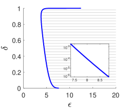
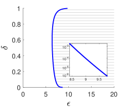
(i) Mechanism Dwork-2014 of Dwork and Roth [2]	(ii) Mechanism Dwork-2006 of Dwork et al. [1]

Figure 1: The shaded area in each subfigure represents the set of $(\epsilon,\delta)$ where Mechanism Dwork-2014 (resp., Dwork-2006) does not achieve $(\epsilon,\delta)$-differential privacy.

The literature’s misuse of the classical Gaussian mechanisms. After a literature review, we find that many papers [12, 13, 14, 15, 16, 17, 7, 8, 18, 19, 20, 21] use the classical Gaussian mechanism Dwork-2006 (resp., Dwork-2014) under values of $\epsilon$ and $\delta$ where Dwork-2006 (resp., Dwork-2014) actually does not achieve $(\epsilon,\delta)$-differential privacy. Table I on Page I summarizes selected papers which misuse the classical Gaussian mechanism Dwork-2006 or Dwork-2014.

Usage of $\epsilon>1$. Although $\epsilon\leq 1$ is preferred in practical applications, there are still cases where $\epsilon>1$ is used, so it is necessary to have Gaussian mechanisms which apply to not only $\epsilon\leq 1$ but also $\epsilon>1$. We discuss usage of $\epsilon>1$ as follows. First, the references [12, 13, 14, 15, 16, 17, 7, 8, 18, 19, 20, 21] in Table I have used $\epsilon>1$. Second, the Differential Privacy Synthetic Data Challenge organized by the National Institute of Standards and Technology (NIST) [41] included experiments of $\epsilon$ as $10$. Third, for a variant of differential privacy called local differential privacy [42] which is implemented in several industrial applications, Apple [43, 44] and Google [45] have adopted $\epsilon>1$.

TABLE I: Misuse of the Classical Gaussian Mechanisms in the Literature from 2014 to 2018.

Selected papers	Mechanism	$\epsilon$	$\delta$	The resulting noise amounts	The least noise amounts
Imtiaz and Sarwate [12]	Dwork-2014	10	0.01	0.3108	0.3501
Liu et al. [13]	Dwork-2014	6, 10	0.1	0.3746, 0.2248	0.3813, 0.2818
Wang et al. [14]	Dwork-2014	8.87, 9.59	$10^{-5}$	0.5462, 0.5052	0.5172, 0.5513
Ermis and Cemgil [15]	Dwork-2014	10	$10^{-2}$, $10^{-5}$	0.3108, 0.4845	0.3501, 0.4999
Liu et al. [16]	Dwork-2014	8	$10^{-1}$	0.2809	0.3215
Imtiaz and Sarwate [17]	Dwork-2014	10	$10^{-2}$	0.3108	0.3501
Jälkö et al. [7]	Dwork-2014	10	$10^{-3}$	0.3776	0.4061
Heikkilä et al. [8]	Dwork-2014	10, 31.62	$10^{-4}$	0.4344, 0.1374	0.1976, 0.4553
Imtiaz and Sarwate [18]	Dwork-2006	10	$10^{-2}$	0.3325	0.3501
Pyrgelis et al. [19]	Dwork-2006	10	$10^{-1}$	0.2448	0.2818
Wang et al. [21]	Dwork-2006	10	$10^{-1}$	0.2448	0.2818
Jain and Thakurta [20]	Dwork-2006	10	$10^{-3}$	0.3898	0.4061

TABLE II: Different mechanisms to achieve $(\epsilon,\delta)$-differential privacy (DP).

DP Mechanisms	Comparison	Common properties
DP-OPT of Theorem 2	• the optimal Gaussian mechanism to achieve $(\epsilon,\delta)$-DP, • no closed-form expression, • computed using the bisection method with the number of iterations being logarithmic in the given error (i.e., tolerance).	Noise amounts $\sigma_{\texttt{DP-OPT}}$, $\sigma_{\texttt{Mechanism-1}}$, and $\sigma_{\texttt{Mechanism-2}}$ are all smaller than $\sigma_{\texttt{Dwork-2014}}$ and $\sigma_{\texttt{Dwork-2006}}$, for $0<\epsilon\leq 1$ which the proofs of Dwork-2014 and Dwork-2006 require (The proof is in Appendix -A).
Our Mechanism 1 of Theorem 4	• closed-form expression involving the complementary error function $\operatorname*{erfc}()$ and its inverse $\operatorname*{inverfc}()$, • computational complexity: dependent on $\operatorname*{erfc}()$ & $\operatorname*{inverfc}()$ implementations and often very efficient, • $\sigma_{\texttt{Mechanism-1}}$ is slightly greater than $\sigma_{\texttt{DP-OPT}}$.
Our Mechanism 2 of Theorem 5	• closed-form expression involving only elementary functions, • computed in constant amount of time, • $\sigma_{\texttt{Mechanism-2}}$ is slightly greater than $\sigma_{\texttt{Mechanism-1}}$.

IV The Optimal Gaussian Mechanism for $(\epsilon,\delta)$-Differential Privacy

A recent work [22] of Balle and Wang in ICML 2018 analyzed the optimal Gaussian mechanism for $(\epsilon,\delta)$-differential privacy, where “optimal” means that the noise amount is the least among Gaussian mechanisms. This optimal Gaussian mechanism is also analyzed by Sommer et al. [46], where the shape of the privacy loss is also discussed. Based on [22], we present Theorem 2 below.

Theorem 2 (Optimal Gaussian mechanism for $(\epsilon,\delta)$-differential privacy).

The optimal Gaussian mechanism for $(\epsilon,\delta)$-differential privacy, denoted by Mechanism DP-OPT, adds Gaussian noise with standard deviation $\sigma_{\texttt{DP-OPT}}$ specified below to each dimension of a query with $\ell_{2}$-sensitivity $\Delta$.

• We derive $\sigma_{\texttt{DP-OPT}}$ as follows based on Theorem 8 of Balle and Wang [22]:

  $$\text{With $a$ satisfying }\operatorname*{erfc}\left(a\right)-e^{\epsilon}\operatorname*{erfc}\left(\sqrt{a^{2}+\epsilon}\right)=2\delta,$$

  $$\text{we get~{}}\textstyle{\sigma_{\texttt{DP-OPT}}:=\frac{\left(a+\sqrt{a^{2}+\epsilon}\hskip 1.5pt\right)\cdot\Delta}{\epsilon\sqrt{2}}},$$ (5)

  where $\operatorname*{erfc}()$ is the complementary error function.

For $\epsilon\geq 0.01$ and $0<\delta\leq 0.05$, we prove the following results:

• $\sigma_{\texttt{DP-OPT}}>\frac{\Delta}{\sqrt{2\epsilon\,}}$.

• $\sigma_{\texttt{DP-OPT}}<\sqrt{2\ln\frac{1}{2\delta}}\cdot\frac{\Delta}{\epsilon}+\frac{\Delta}{\sqrt{2\epsilon\,}}$.

Remark 3.

Results (ii) and (iii) of Theorem 2 mean that $\sigma_{\texttt{DP-OPT}}$ is in the form of $\Theta\left(\frac{1}{\sqrt{\epsilon}}\right)$ for large $\epsilon$ (note $\frac{1}{\epsilon}$ is smaller than $\frac{1}{\sqrt{\epsilon}}$ for large $\epsilon$). This further implies the result of Theorem 1 for $0<\delta\leq 0.05$ (our direct proof for Theorem 1 in Appendix -B works for any $0<\delta<1$).

Remark 4.

With $r(u):=\operatorname*{erfc}\left(u\right)-e^{\epsilon}\operatorname*{erfc}\left(\sqrt{u^{2}+\epsilon}\right)$, the term $a$ in Eq. (5) satisfies $r(a)=2\delta$. Then $r(u)$ strictly decreases as $u$ increases given the derivative $r^{\prime}(u)=\frac{2}{\sqrt{\pi}}\exp(-u^{2})\times\frac{u-\sqrt{u^{2}+\epsilon}}{\sqrt{u^{2}+\epsilon}}<0$. Based on this and $r(0)=1-e^{\epsilon}\operatorname*{erfc}\left(\sqrt{\epsilon}\right)$, for $a$ in Eq. (5), we obtain $a>0$ if $2\delta<1-e^{\epsilon}\operatorname*{erfc}\left(\sqrt{\epsilon}\right)$, and $a\leq 0$ otherwise. More discussions about Remark 4 are presented in Appendix -D of this supplementary file.

Remark 5.

Mechanism DP-OPT is just the optimal Gaussian mechanism for $(\epsilon,\delta)$-differential privacy in the sense that it gives the minimal required amount of noise when the noise follows a Gaussian distribution. However, it may not be the optimal mechanism for $(\epsilon,\delta)$-differential privacy, since there may exist other perturbation methods [35, 32, 47] which may outperform a Gaussian mechanism under certain utility measure [33].

We prove Theorem 2 in Appendix -C of this supplementary file.

Since $\sigma_{\texttt{DP-OPT}}$ of Theorem 2 has no closed-form expression and needs to be approximated in an iterative manner, we first provide its asympotics in Theorem 3 and present more computationally efficient upper bounds for $\sigma_{\texttt{DP-OPT}}$ in Section V.

In Appendix -O of this supplementary file, we present Algorithm 1 to compute $\sigma_{\texttt{DP-OPT}}$ of Theorem 2.

We now analyze the asympotics for the optimal Gaussian noise amount $\sigma_{\texttt{DP-OPT}}$ of $(\epsilon,\delta)$-differential privacy. As a side result, we prove that $\sigma_{\texttt{DP-OPT}}$ is always less than $\frac{\Delta}{2\sqrt{2}\cdot\operatorname*{inverf}(\delta)}$ and hence bounded even for $\epsilon\to 0$. This is in contrast to the classical Gaussian mechanisms’ noise amounts $\sigma_{\texttt{Dwork-2006}}$ and $\sigma_{\texttt{Dwork-2014}}$ in Eq. (1) and (2) which scale with $\frac{1}{\epsilon}$ and hence tend to $\infty$ as $\epsilon\to 0$.

Theorem 3 (An upper bound and asympotics of the optimal Gaussian noise amount for $(\epsilon,\delta)$-differential privacy).

• For any $\epsilon>0$ and $0<\delta<1$, $\sigma_{\texttt{DP-OPT}}$ is less than $\frac{\Delta}{2\sqrt{2}\cdot\operatorname*{inverf}(\delta)}$, which is the optimal Gaussian noise amount to achieve $(0,\delta)$-differential privacy.

• Given a fixed $0<\delta<1$, $\sigma_{\texttt{DP-OPT}}$ converges to its upper bound $\frac{\Delta}{2\sqrt{2}\cdot\operatorname*{inverf}(\delta)}$ as $\epsilon\to 0$.

• Given a fixed $0<\delta<1$, $\sigma_{\texttt{DP-OPT}}$ is $\Theta\left(\frac{1}{\sqrt{\epsilon}}\right)$ as $\epsilon\to\infty$; specifically, $\lim_{\epsilon\to\infty}\sigma_{\texttt{DP-OPT}}\Big{/}\left(\frac{\Delta}{\sqrt{2\epsilon\hskip 1.5pt}}\right)=1$.

• Given a fixed $\epsilon>0$, $\sigma_{\texttt{DP-OPT}}$ is $\Theta\left(\sqrt{\ln\frac{1}{\delta}}\right)$ as $\delta\to 0$; specifically, $\lim_{\delta\to 0}\sigma_{\texttt{DP-OPT}}\Big{/}\left(\frac{\Delta}{\epsilon}\sqrt{2\ln\frac{1}{\delta}}\hskip 1.5pt\right)=1$.

Intuition of Result ① of Theorem 3 based on Theorem 2. With $\delta$ fixed, when $\epsilon$ tends to 0, the quantity $a$ in Eq. (5) of Theorem 2 is negative and is close to $-\operatorname*{inverfc}(1-\delta)$; i.e., $\operatorname*{inverf}(\delta)$, where we use $\operatorname*{erfc}\left(-a\right)=2-\operatorname*{erfc}\left(a\right)$. Then the numerator $(a+\sqrt{a^{2}+\epsilon})\Delta$ of Eq. (5) can be written as $\frac{\epsilon\Delta}{-a+\sqrt{a^{2}+\epsilon}}$ and approaches $\frac{\epsilon\Delta}{(-a)\cdot 2}$ to scale with $\epsilon$ instead of scaling with $\sqrt{\epsilon}$ as $\epsilon\to 0$. As the numerator and denominator of Eq. (5) are both $\Theta(\epsilon)$ as $\epsilon\to 0$, $\sigma_{\texttt{DP-OPT}}$ with fixed $\delta$ does not grow unboundedly as $\epsilon\to 0$.

We prove Theorem 3 in Appendix -E of this supplementary file. Theorem 3 provides the first asymptotic results in the literature on the optimal Gaussian noise amount for $(\epsilon,\delta)$-differential privacy. The proofs delicately bound $\sigma_{\texttt{DP-OPT}}$ to avoid over-approximation.

For clarification, we note that Results ② and ④ of Theorem 3 do not contradict each other since Result ② fixes $0<\delta<1$ and considers $\epsilon\to 0$ so that $\epsilon/\delta\to 0$, while Result ④ fixes $\epsilon>0$ and considers $\delta\to 0$ so that $\delta/\epsilon\to 0$. More specifically, to bound $\sigma_{\texttt{DP-OPT}}$ in Result ④, we consider $\epsilon>f(\delta)$ for some function $f$, which clearly holds given a fixed $\epsilon>0$ and $\delta\to 0$. With $\epsilon>f(\delta)$, the expression $\frac{\Delta}{\epsilon}\sqrt{2\ln\frac{1}{\delta}}$ in Result ④ is less than $\frac{\Delta}{f(\delta)}\sqrt{2\ln\frac{1}{\delta}}$, which is less than $\frac{\Delta}{2\sqrt{2}\cdot\operatorname*{inverf}(\delta)}$ for suitable $f(\delta)$, so Result ② does not contradict Result ④.

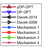
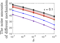
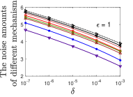
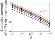
	(i)	(ii)	(iii)
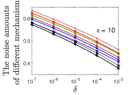
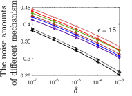
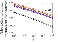
	(iv)	(v)	(vi)

Figure 2: The noise amounts of different mechanisms with respect to $\delta$, for $\epsilon$ = 0.1, 1, 5, 10, 15 and 20. The meanings of the legends are as follows.

• pDP-OPT (resp., DP-OPT) is the optimal Gaussian mechanism to achieve $(\epsilon,\delta)$-pDP (resp., $(\epsilon,\delta)$-DP), where pDP is short for probabilistic differential privacy, a notion stronger than differential privacy (DP) and to be elaborated in Section VI.

• Dwork-2006 (resp., Dwork-2014) is the Gaussian mechanism proposed by Dwork et al. [1] in 2006 (resp., Dwork and Roth [2] in 2014) to achieve $(\epsilon,\delta)$-DP.

• Mechanism 1 and Mechanism 2, which are our proposals to achieve $(\epsilon,\delta)$-DP and discussed in Section V, are simpler and more computationally efficient than DP-OPT.

• Mechanism 3 and Mechanism 4, which are our proposals to achieve $(\epsilon,\delta)$-pDP and will be discussed in Section VI-D, are simpler and more computationally efficient than pDP-OPT.

V Our Proposed Gaussian Mechanisms for $(\epsilon,\delta)$-Differential Privacy

Table II summarizes different mechanisms to achieve $(\epsilon,\delta)$-differential privacy (DP), including DP-OPT in Theorem 2 of the previous section as well as our Mechanism 1 and Mechanism 2 to be presented below.

We now detail our Gaussian mechanisms for $(\epsilon,\delta)$-differential privacy, where the noise amounts have closed-form expressions and are more computationally efficient than the above Theorem 2’s DP-OPT which has no closed-form expression. Our idea is to present computationally efficient upper bounds of $\sigma_{\texttt{DP-OPT}}$. To this end, we first present Lemma 1, which upper bounds $a$ in Eq. (5) of Theorem 2.

Lemma 1.

$a$ in Eq. (5) is less than $b$ in Eq. (7a).

We prove Lemma 1 in Appendix -G of this supplementary file. Theorem 2 and Lemma 1 imply

$$\text{$\sigma_{\texttt{DP-OPT}}$ in Eq.~{}(\ref{eqn-sigma-DP-OPT})}<\text{$\sigma_{\texttt{Mechanism-1}}$ in Eq.~{}(\ref{eqn-sigma-Mechanism-1}) of Theorem~{}\ref{thm-Mechanism-1}},$$ (6)

where Theorem 4 below presents Mechanism 1 to achieve $(\epsilon,\delta)$-differential privacy.

Theorem 4 (Gaussian Mechanism 1 for $(\epsilon,\delta)$-differential privacy).

$(\epsilon,\delta)$-Differential privacy can be achieved by Mechanism 1, which adds Gaussian noise with standard deviation $\sigma_{\texttt{Mechanism-1}}$ to each dimension of a query with $\ell_{2}$-sensitivity $\Delta$, for $\sigma_{\texttt{Mechanism-1}}$ given by

$$b:=\begin{cases}{\operatorname*{inverfc}\left(\frac{2\delta}{1-e^{\epsilon}\cdot\frac{\operatorname*{erfc}\left(\sqrt{\big{[}\operatorname*{inverfc}\big{(}2\delta+e^{\epsilon}\operatorname*{erfc}\left(\sqrt{\epsilon}\right)\big{)}\big{]}^{2}+\epsilon}\right)}{2\delta+e^{\epsilon}\operatorname*{erfc}\left(\sqrt{\epsilon}\right)}}\right)}\\ \text{~{}if $2-e^{\epsilon}\operatorname*{erfc}\left(\sqrt{\epsilon}\right)>2\delta$,}\\ 0\text{~{}otherwise};\end{cases}$$ (7a)

$$\textstyle{\sigma_{\texttt{Mechanism-1}}:=\frac{\left(b+\sqrt{b^{2}+\epsilon}\hskip 1.5pt\right)\cdot\Delta}{\epsilon\sqrt{2}}}.$$ (7b)

The expression of $\sigma_{\texttt{Mechanism-1}}$ involves the complementary error function $\operatorname*{erfc}()$ and its inverse $\operatorname*{inverfc}()$. Hence, we further present Lemma 2 below, which will enable us to propose Mechanism 2. Its noise amount is given by the closed-form expression of $\sigma_{\texttt{Mechanism-2}}$ and has only elementary functions.

Lemma 2 upper bounds $b$ in Eq. (7a) of Theorem 4.

Lemma 2.

$b$ in Eq. (7a) is less than $c$ in Eq. (9).

We prove Lemma 2 in Appendix -H of this supplementary file. Theorem 4 and Lemma 2 imply

$$\text{$\sigma_{\texttt{Mechanism-1}}$ in Eq.~{}(\ref{eqn-sigma-Mechanism-1})}<\text{$\sigma_{\texttt{Mechanism-2}}$ in Eq.~{}(\ref{eqn-u-Mechanism-2})},$$ (8)

where the presented Mechanism 2 in Theorem 5 below is further simpler than Mechanism 1 as noted above.

Theorem 5 (Gaussian Mechanism 2 for $(\epsilon,\delta)$-differential privacy).

For $0<\delta<0.5$, $(\epsilon,\delta)$-differential privacy can be achieved by Mechanism 2, which adds Gaussian noise with standard deviation $\sigma_{\texttt{Mechanism-2}}$ to each dimension of a query with $\ell_{2}$-sensitivity $\Delta$, for $\sigma_{\texttt{Mechanism-2}}$ given by

$$\textstyle{c:=\sqrt{\ln\frac{2}{\sqrt{16\delta+1}-1}}};~{}~{}\textstyle{\sigma_{\texttt{Mechanism-2}}:=\frac{\left(c+\sqrt{c^{2}+\epsilon}\hskip 1.5pt\right)\cdot\Delta}{\epsilon\sqrt{2}}}.$$ (9)

Superiority of our mechanisms. The following discussions show the superiority of our proposed mechanisms.

• From Inequalities (6) and (8), we have $\text{$\sigma_{\texttt{DP-OPT}}$ in Eq.~{}(\ref{eqn-sigma-DP-OPT})}<\text{$\sigma_{\texttt{Mechanism-1}}$ in Eq.~{}(\ref{eqn-sigma-Mechanism-1})}<\text{$\sigma_{\texttt{Mechanism-2}}$ in Eq.~{}(\ref{eqn-u-Mechanism-2})}$. Among these noise amounts, $\sigma_{\texttt{Mechanism-1}}$ and $\sigma_{\texttt{Mechanism-2}}$ are straightforward to compute, whereas $\sigma_{\texttt{DP-OPT}}$ require higher computational complexity (a simple approach is the bisection method in [48, Page 3]. Also, our plots in Figure 2 show that the noise amounts added by the optimal Gaussian mechanism DP-OPT and our more computationally efficient Mechanism 1 are close.

• For $0<\epsilon\leq 1$ where the proofs of Dwork-2006 of [1] and Dwork-2014 of [2] require, we prove in Appendix -A that

  $$\sigma_{\texttt{Mechanism-1}}<\sigma_{\texttt{Mechanism-2}}<\sigma_{\texttt{Dwork-2014}}<\sigma_{\texttt{Dwork-2006}}.$$ (10)

• From Theorem 1, there exists a function $G(\delta)$ such that Dwork-2014 does not achieve $(\epsilon,\delta)$-differential privacy for $\epsilon>G(\delta)$. Figure 1 shows $G(10^{-3})=7.47$, $G(10^{-4})=8.00$, $G(10^{-5})=8.43$, and $G(10^{-6})=8.79$. Result ii) above considers $0<\epsilon\leq 1$. For $1<\epsilon\leq G(\delta)$ which the proof of Dwork-2014 does not cover but Dwork-2014 happens to achieve $(\epsilon,\delta)$-differential privacy, $\sigma_{\texttt{Mechanism-1}}<\sigma_{\texttt{Dwork-2014}}$ still holds as given by Figure 2. Moreover, our Mechanism 1 and Mechanism 2 apply to any $\epsilon$. A similar discussion holds for Dwork-2006.

Applications of our mechanisms. Our proposed mechanisms has the following applications. First, the noise amounts of our mechanisms can be set as initial values to quickly search for the optimal value or its tighter upper bound (as the optimal value has no closed-form expression). We use such approach in Algorithm 1 of Appendix -O of this supplementary file. In addition, our upper bounds may provide an intuitive understanding about how a sufficient Gaussian noise amount changes according to $\epsilon$ and $\delta$: given $\delta$, a noise amount of $\Theta\big{(}\frac{1}{\epsilon}\big{)}+\Theta\big{(}\frac{1}{\sqrt{\epsilon}}\big{)}$ suffices; i.e., $\Theta\big{(}\frac{1}{\epsilon}\big{)}$ suffices for small $\epsilon$ and $\Theta\big{(}\frac{1}{\sqrt{\epsilon}}\big{)}$ suffices for large $\epsilon$. Finally, our mechanisms can be useful for Internet of Things (IoT) devices with little power or computational capabilities, since our mechanisms are more computationally efficient than the optimal Gaussian mechanism.

VI $(\epsilon,\delta)$-Probabilistic Differential Privacy: Connection to $(\epsilon,\delta)$-Differential Privacy and Gaussian Mechanisms

In this section, for $(\epsilon,\delta)$-probabilistic differential privacy, we discuss its connection to $(\epsilon,\delta)$-differential privacy and its Gaussian mechanisms.

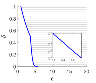
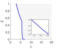
(i) Mechanism Dwork-2014	(ii) Mechanism Dwork-2006

Figure 3: The shaded area in each subfigure represents the set of $(\epsilon,\delta)$ where Mechanism Dwork-2014 (resp., Dwork-2006) does not achieve $(\epsilon,\delta)$-probabilistic differential privacy.

VI-A $(\epsilon,\delta)$-Probabilistic differential privacy

To achieve $(\epsilon,\delta)$-differential privacy (formally given in Definition 1 on Page 1), most mechanisms ensure a condition on the privacy loss random variable defined below. Such condition is termed $(\epsilon,\delta)$-probabilistic differential privacy [40] and elaborated below. We will explain that $(\epsilon,\delta)$-probabilistic differential privacy is sufficient but not necessary for $(\epsilon,\delta)$-differential privacy.

For neighboring datasets $D$ and $D^{\prime}$, the privacy loss $L_{Y,D,D^{\prime}}(y)$ represents the multiplicative difference between the probabilities that the same output $y$ is observed when the randomized algorithm $Y$ is applied to $D$ and $D^{\prime}$, respectively. Specifically, we define

$$L_{Y,D,D^{\prime}}(y):=\ln\frac{{\mathbb{F}}\left[{Y(D)=y}\right]}{{\mathbb{F}}\left[{Y(D^{\prime})=y}\right]},$$ (11)

where ${\mathbb{F}}\left[{\cdot}\right]$ denotes the probability density function.

For simplicity, we use probability density function ${\mathbb{F}}\left[{\cdot}\right]$ in Eq. (11) above by assuming that the randomized algorithm $Y$ has continuous output. If $Y$ has discrete output, we replace ${\mathbb{F}}\left[{\cdot}\right]$ by probability notation ${\mathbb{P}}\left[{\cdot}\right]$.

When $y$ follows the probability distribution of random variable $Y(D)$, $L_{Y,D,D^{\prime}}(y)$ follows the probability distribution of $L_{Y,D,D^{\prime}}(Y(D))$, which is the privacy loss random variable. As a sufficient condition to enforce $(\epsilon,\delta)$-differential privacy, $(\epsilon,\delta)$-probabilistic differential privacy of [40] is defined such that the privacy loss random variable $L_{Y,D,D^{\prime}}(Y(D))$ falls in the interval $[-\epsilon,\epsilon]$ with probability at least $1-\delta$; i.e., $\mathbb{P}\left[-\epsilon\leq L_{Y,D,D^{\prime}}(Y(D))\leq\epsilon\right]\geq 1-\delta$. This is equivalent to the following definition.

Definition 2 ($(\epsilon,\delta)$-Probabilistic differential privacy [40]).

A randomized algorithm $Y$ satisfies $(\epsilon,\delta)$-probabilistic differential privacy, if for any two neighboring datasets $D$ and $D^{\prime}$ (elaborated in Remark 1 on Page 1), we have that for $y$ following the probabilistic distribution of the output $Y(D)$ (notated as $y\sim Y(D)$),

$$\mathbb{P}_{y\sim Y(D)}\left[e^{-\epsilon}\leq\frac{{\mathbb{F}}\left[{Y(D)=y}\right]}{{\mathbb{F}}\left[{Y(D^{\prime})=y}\right]}\leq e^{\epsilon}\right]\geq 1-\delta,$$ (12)

where ${\mathbb{F}}\left[{\cdot}\right]$ denotes the probability density function.

VI-B Relationships between differential privacy and probabilistic differential privacy

Lemmas 3 and 4 below present the relationships between differential privacy and probabilistic differential privacy.

Lemma 3.

$(\epsilon,\delta)$-Probabilistic differential privacy implies $(\epsilon,\delta)$-differential privacy.

Lemma 4.

$(\epsilon,\delta)$-Differential privacy implies $(\epsilon_{*},\frac{\delta\cdot(1+e^{-\epsilon_{*}})}{1-e^{\epsilon-\epsilon_{*}}})$-probabilistic differential privacy for any $\epsilon_{*}>\epsilon$.

While the straightforward Lemma 3 is shown in [2], the proof of Lemma 4 is not trivial. Although [9] of Dwork and Rothblum, and [10] of Bun and Steinke mention that differential privacy is equivalent, up to a small loss in parameters, to probabilistic differential privacy, [9, 10] do not present Lemma 4. For completeness, we present the proofs of Lemmas 3 and 4 in Appendices -I and -J of this supplementary file.

Similar to Theorem 1 on Page 1, we show in Figure 3 the failures of the classical Gaussian mechanisms of Dwork and Roth [2] in 2014 and of Dwork et al. [1] in 2006 to achieve $(\epsilon,\delta)$-probabilistic differential privacy for large $\epsilon$.

We now present the optimal Gaussian mechanism for $(\epsilon,\delta)$-probabilistic differential privacy.

TABLE III: Different mechanisms to achieve $(\epsilon,\delta)$-probabilistic differential privacy (pDP).

pDP Mechanisms	Comparison
Our pDP-OPT of Theorem 6	• the optimal Gaussian mechanism to achieve $(\epsilon,\delta)$-pDP, • no closed-form expression, • computed using the bisection method with the number of iterations being logarithmic in the given error (i.e., tolerance).
Our Mechanism 3 of Theorem 8	• closed-form expression involving the complementary error function’s inverse $\operatorname*{inverfc}()$, • computational complexity: dependent on $\operatorname*{inverfc}()$ implementations and often very efficient, • $\sigma_{\texttt{Mechanism-3}}$ is slightly greater than $\sigma_{\texttt{pDP-OPT}}$.
Our Mechanism 4 of Theorem 9	• closed-form expression involving only elementary functions, • computed in constant amount of time, • $\sigma_{\texttt{Mechanism-4}}$ is slightly greater than $\sigma_{\texttt{Mechanism-3}}$.

VI-C An analytical but not closed-form expression for the optimal Gaussian mechanism of $(\epsilon,\delta)$-probabilistic differential privacy

The optimal Gaussian mechanism of $(\epsilon,\delta)$-probabilistic differential privacy (pDP) is given in Theorem 6 below.

Theorem 6 (Optimal Gaussian mechanism for $(\epsilon,\delta)$-probabilistic differential privacy).

The optimal Gaussian mechanism for $(\epsilon,\delta)$-probabilistic differential privacy, denoted by Mechanism pDP-OPT, adds Gaussian noise with standard deviation $\sigma_{\texttt{pDP-OPT}}$ to each dimension of a query with $\ell_{2}$-sensitivity $\Delta$, for $\sigma_{\texttt{pDP-OPT}}$ given by

$$\text{Solve $d$ such that }\operatorname*{erfc}\left(d\right)+\operatorname*{erfc}\left(\sqrt{d^{2}+\epsilon}\right)=2\delta;$$ (13a)

$$\sigma_{\texttt{pDP-OPT}}:=\frac{\left(d+\sqrt{d^{2}+\epsilon}\hskip 1.5pt\right)\cdot\Delta}{\epsilon\sqrt{2}}.$$ (13b)

Remark 6.

Mechanism pDP-OPT is just the optimal Gaussian mechanism for $(\epsilon,\delta)$-probabilistic differential privacy in the sense that it gives the minimal required amount of noise when the noise follows a Gaussian distribution. However, it may not be the optimal mechanism for $(\epsilon,\delta)$-probabilistic differential privacy, since there may exist other perturbation methods (e.g., adding non-Gaussian noise) which may outperform a Gaussian mechanism under certain utility measure [47].

We prove Theorem 6 in Appendix -K of this supplementary file. We present the asympotics of $\sigma_{\texttt{pDP-OPT}}$ as Theorem 7 below.

Theorem 7 (The asympotics of the optimal Gaussian noise amount for $(\epsilon,\delta)$-probabilistic differential privacy).

• Given a fixed $0<\delta<1$, $\sigma_{\texttt{pDP-OPT}}$ is $\Theta\left(\frac{1}{\epsilon}\right)$ as $\epsilon\to 0$. Specifically, given a fixed $0<\delta<1$, $\lim_{\epsilon\to 0}\sigma_{\texttt{pDP-OPT}}\Big{/}\left(\frac{\operatorname*{inverfc}(\delta)\cdot\Delta}{\epsilon\sqrt{2}}\right)=1$.

• Given a fixed $0<\delta<1$, $\sigma_{\texttt{pDP-OPT}}$ is $\Theta\left(\frac{1}{\sqrt{\epsilon}}\right)$ as $\epsilon\to\infty$. Specifically, given a fixed $0<\delta<1$, $\lim_{\epsilon\to\infty}\sigma_{\texttt{pDP-OPT}}\Big{/}\left(\frac{\Delta}{\sqrt{2\epsilon\hskip 1.5pt}}\right)=1$.

• Given a fixed $\epsilon>0$, $\sigma_{\texttt{pDP-OPT}}$ is $\Theta\left(\sqrt{\ln\frac{1}{\delta}}\right)$ as $\delta\to 0$. Specifically, given a fixed $\epsilon>0$, $\lim_{\delta\to 0}\sigma_{\texttt{pDP-OPT}}\Big{/}\left(\frac{\Delta}{\epsilon}\sqrt{2\ln\frac{1}{\delta}}\hskip 1.5pt\right)=1$.

Theorem 7 is proved in Appendix -L of this supplementary file.

Remark 7.

From Result ① of Theorem 7, given a fixed $0<\delta<1$, $\sigma_{\texttt{pDP-OPT}}=\Theta\left(\frac{1}{\epsilon}\right)\to\infty$ as $\epsilon\to 0$. In contrast, from Result ① of Theorem 3, given a fixed $0<\delta<1$, $\sigma_{\texttt{DP-OPT}}\to\frac{\Delta}{2\sqrt{2}\cdot\operatorname*{inverf}(\delta)}$ as $\epsilon\to 0$. This shows a fundamental difference between $(\epsilon,\delta)$-differential privacy and $(\epsilon,\delta)$-probabilistic differential privacy.

Remark 8.

In Lemmas 3 and 4 above, we show the relationship between differential privacy and probabilistic differential privacy that the latter implies the former and the former implies the latter up to possible loss in privacy parameters. Given this, one may wonder if this relationship contradicts their difference discussed in Remark 7 above as $\epsilon\to 0$. Below we explain there is no contradiction, by showing that the Gaussian noise amount for probabilistic differential privacy obtained by first achieving differential privacy is at the same order as the optimal Gaussian noise amount for probabilistic differential privacy when $\epsilon\to 0$.

From Lemma 4, $(0,\frac{\delta\cdot(1-e^{-\epsilon})}{1+e^{-\epsilon}})$-differential privacy implies $(\epsilon,\delta)$-probabilistic differential privacy. From Result ① of Theorem 3, $(0,\frac{\delta\cdot(1-e^{-\epsilon})}{1+e^{-\epsilon}})$-differential privacy can be achieved by the Gaussian mechanism with noise amount $\frac{\Delta}{2\sqrt{2}\cdot\operatorname*{inverf}\big{(}\frac{\delta\cdot(1-e^{-\epsilon})}{1+e^{-\epsilon}}\big{)}}$. Hence, $(\epsilon,\delta)$-probabilistic differential privacy can also be achieved by the Gaussian mechanism with noise amount $\frac{\Delta}{2\sqrt{2}\cdot\operatorname*{inverf}\big{(}\frac{\delta\cdot(1-e^{-\epsilon})}{1+e^{-\epsilon}}\big{)}}$, which given $\delta$ is $\Theta\left(\frac{1}{\epsilon}\right)$ as $\epsilon\to 0$ due to $\lim_{\epsilon\to 0}\frac{(1-e^{-\epsilon})}{1+e^{-\epsilon}}\big{/}\epsilon=\frac{1}{2}$ and $\lim_{x\to 0}\frac{\operatorname*{inverf}(x)}{x}=\frac{\sqrt{\pi}}{2}$ from [49]. From Result ① of Theorem 7, the optimal Gaussian noise amount for $(\epsilon,\delta)$-probabilistic differential privacy given $\delta$ is also $\Theta\left(\frac{1}{\epsilon}\right)$ as $\epsilon\to 0$. Hence, the combination of Lemma 4 and Result ① of Theorem 3 does not contradict Result ① of Theorem 7.

From Theorem 6, the optimal Gaussian mechanism pDP-OPT does not have a closed-form expression. In the next subsection, we detail our Gaussian mechanisms for $(\epsilon,\delta)$-pDP, where the noise amounts have closed-form expressions and are more computationally efficient than pDP-OPT.

VI-D Our Gaussian mechanisms for $(\epsilon,\delta)$-probabilistic differential privacy with closed-form expressions of noise amounts

The idea of our Gaussian mechanisms is to present computationally efficient upper bounds of $\sigma_{\texttt{pDP-OPT}}$. To this end, we first present Lemma 5, which upper bounds $d$ in Eq. (13a) of Theorem 6.

Lemma 5.

$d$ in Eq. (13a) is greater than $\operatorname*{inverfc}(2\delta)$ and less than $\operatorname*{inverfc}(\delta)$.

We prove Lemma 5 in Appendix -M of this supplementary file. Theorem 6 and Lemma 5 imply an upper bound of $\sigma_{\texttt{pDP-OPT}}$ as $\sigma_{\texttt{Mechanism-3}}$ in Theorem 8 below, where we present Mechanism 3 to achieve $(\epsilon,\delta)$-probabilistic differential privacy.

Theorem 8 (Gaussian Mechanism 3 for $(\epsilon,\delta)$-Probabilistic differential privacy).

$(\epsilon,\delta)$-Probabilistic differential privacy can be achieved by Mechanism 3, which adds Gaussian noise with standard deviation $\sigma_{\texttt{Mechanism-3}}$ to each dimension of a query with $\ell_{2}$-sensitivity $\Delta$, for $\sigma_{\texttt{Mechanism-3}}$ given by

$$f:=\operatorname*{inverfc}(\delta);$$ (14a)

$$\sigma_{\texttt{Mechanism-3}}:=\frac{\left(f+\sqrt{f^{2}+\epsilon}\hskip 1.5pt\right)\cdot\Delta}{\epsilon\sqrt{2}}.$$ (14b)

The expression of $\sigma_{\texttt{Mechanism-3}}$ involves the complementary error function’s inverse $\operatorname*{inverfc}()$. Hence, we further present Lemma 6 below, which will enable us to propose Mechanism 4. Its noise amount is given by the closed-form expression of $\sigma_{\texttt{Mechanism-4}}$ and has only elementary functions.

Lemma 6 upper bounds $f$ in Eq. (14a).

Lemma 6.

$f$ in Eq. (14a) is less than $g$ in Eq. (15a).

We prove Lemma 6 in Appendix -N of this supplementary file.

Theorem 8 and Lemma 6 imply an upper bound of $\sigma_{\texttt{Mechanism-3}}$ as $\sigma_{\texttt{Mechanism-4}}$ in Theorem 9 below, where the presented Mechanism 4 is further simpler than Mechanism 3 as noted above.

Theorem 9 (Gaussian Mechanism 4 for $(\epsilon,\delta)$-Probabilistic differential privacy).

$(\epsilon,\delta)$-Probabilistic differential privacy can be achieved by Mechanism 4, which adds Gaussian noise with standard deviation $\sigma_{\texttt{Mechanism-4}}$ to each dimension of a query with $\ell_{2}$-sensitivity $\Delta$, for $\sigma_{\texttt{Mechanism-4}}$ given by

$$g:=\sqrt{\ln\frac{2}{\sqrt{8\delta+1}-1}};$$ (15a)

$$\sigma_{\texttt{Mechanism-4}}:=\frac{\left(g+\sqrt{g^{2}+\epsilon}\hskip 1.5pt\right)\cdot\Delta}{\epsilon\sqrt{2}}.$$ (15b)

Table III summarizes different mechanisms to achieve $(\epsilon,\delta)$-probabilistic differential privacy discussed above.

VII Concentrated Differential Privacy and Related Notions

Several variants of differential privacy (DP), including mean-concentrated differential privacy (mCDP) [9], zero-concentrated differential privacy (zCDP) [10], Rényi differential privacy [23] (RDP), and truncated concentrated differential privacy (tCDP) [24] have been recently proposed as alternatives to $(\epsilon,\delta)$-DP. Below we show that achieving $(\epsilon,\delta)$-DP by first ensuring one of these privacy definitions (mCDP, zCDP, RDP, and tCDP) cannot give Gaussian mechanisms better than ours, based on existing results on the relationships between mCDP, zCDP, RDP, tCDP and DP.

Lemma 7 (Relationship between $(\epsilon,\delta)$-DP and $(\mu,\tau)$-mCDP).

For $\epsilon>\mu$, $(\mu,\tau)$-mCDP implies $(\epsilon,\delta)$-probabilistic differential privacy (pDP) for
$\delta=\exp\left(-\frac{(\epsilon-\mu)^{2}}{2\tau^{2}}\right)+\exp\left(-\frac{(\epsilon+\mu)^{2}}{2\tau^{2}}\right)$, which further implies $(\epsilon,\delta)$-DP.

Despite not being presented in [9] which proposes mCDP, the first part of Lemma 7 clearly follows from the definitions of mCDP and pDP by using the tail bounds on the privacy loss random variable of mCDP, while the second part of Lemma 7 is from Lemma 3.

For a query with $\ell_{2}$-sensitivity $1$, Theorem 3.2 in [9] shows that the Gaussian mechanism with standard deviation $\sigma$ achieves $(\frac{1}{2\sigma^{2}},\frac{1}{\sigma})$-mCDP, which based on Lemma 7 implies $(\epsilon,\delta)$-pDP for $\delta=\exp\left(-\frac{(\epsilon-\frac{1}{2\sigma^{2}})^{2}}{2(\frac{1}{\sigma})^{2}}\right)+\exp\left(-\frac{(\epsilon+\frac{1}{2\sigma^{2}})^{2}}{2(\frac{1}{\sigma})^{2}}\right)$. Expressing $\sigma$ in terms of $\epsilon$ and $\delta$ gives $\sigma$ as $\sigma_{\texttt{pDP-OPT}}$ of Theorem 6. Hence, using the relationship between mCDP and (p)DP does not give a new mechanism which we have not presented.

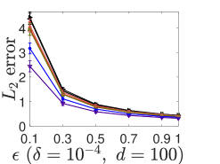
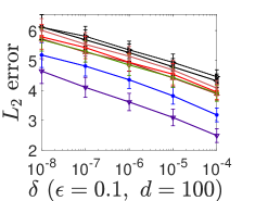
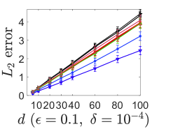
(a) Error w.r.t. $\epsilon$	(b) Error w.r.t. $\delta$	(c) Error w.r.t. dimension $d$

Figure 4: Mean estimation.

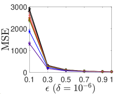
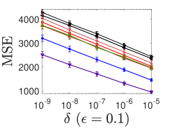
(a) Error w.r.t. $\epsilon$	(b) Error w.r.t. $\delta$

Figure 5: Histogram estimation.

Relationship between zCDP and DP. From Proposition 1.3 and Proposition 1.6 in [10], $\rho$-zCDP implies ($\epsilon$, $\delta$)-DP for $\epsilon=\rho+2\sqrt{\rho\ln(\frac{1}{\delta})}$. Moreover, the Gaussian mechanism with standard deviation $\sigma$ achieves $\rho$-zCDP by [10], where $\rho=\frac{\Delta^{2}}{2\sigma^{2}}$. Combining these results, we can derive that the Gaussian mechanism with standard deviation $\frac{\Delta\cdot\left(\sqrt{\ln\frac{1}{\delta}}+\sqrt{\ln\frac{1}{\delta}+\epsilon}\right)}{\sqrt{2}\epsilon}$ achieves ($\epsilon$, $\delta$)-DP. This expression is obtained by solving $\sigma$ which satisfy $\rho=\frac{\Delta^{2}}{2\sigma^{2}}$ and $\epsilon=\rho+2\sqrt{\rho\ln(\frac{1}{\delta})}$. Such noise amount is even worse (i.e., higher) than our weakest Mechanism 4 in Theorem 9 on Page 9 in view of $\sqrt{8\delta+1}-1>2\delta$ given $0<\delta<1$. Hence, achieving $(\epsilon,\delta)$-DP by first ensuring zCDP cannot give Gaussian mechanisms better than ours.

Relationship between RDP and DP. Mironov [23] shows that ($\alpha$, $\rho\alpha$)-RDP implies ($\epsilon$, $\delta$)-DP for $\epsilon=\rho\alpha+\frac{\ln(1/\delta)}{\alpha-1}$, and the Gaussian mechanism with standard deviation $\sigma$ achieves ($\alpha,\rho\alpha$)-RDP for $\rho=\frac{\Delta^{2}}{2\sigma^{2}}$. Combining these results, we can also prove that the Gaussian mechanism with standard deviation $\frac{\Delta\cdot\left(\sqrt{\ln\frac{1}{\delta}}+\sqrt{\ln\frac{1}{\delta}+\epsilon}\right)}{\sqrt{2}\,\epsilon}$ achieves ($\epsilon$, $\delta$)-DP. This expression is obtained by finding the smallest $\sigma$ such that there exists $\alpha>1$ such that $\rho=\frac{\Delta^{2}}{2\sigma^{2}}$ and $\epsilon=\rho\alpha+\frac{\ln(1/\delta)}{\alpha-1}$ (we just express $\sigma$ and take its minimum with respect to $\alpha$). As noted above, this noise amount is even worse (i.e., higher) than our weakest Mechanism 4 in Theorem 9. Thus, achieving $(\epsilon,\delta)$-DP by first ensuring RDP cannot give Gaussian mechanisms better than ours. We emphasize that the comparison may be different if the RDP paper [23]’s Proposition 3 that ($\alpha$, $\rho\alpha$)-RDP implies ($\rho\alpha+\frac{\ln(1/\delta)}{\alpha-1}$, $\delta$)-DP can be improved. Yet, we have not been able to find such improvement after checking prior papers related to RDP.

Relationship between tCDP and DP. Bun et al. [24] show that ($\rho,~{}\omega$)-tCDP implies ($\epsilon$, $\delta$)-DP for $\epsilon=\begin{cases}\rho+2\sqrt{\rho\ln{\frac{1}{\delta}}}~{}\textit{if}~{}\ln\frac{1}{\delta}\leq(\omega-1)^{2}\rho,\\ \rho\omega+\frac{\ln(\frac{1}{\delta})}{\omega-1}~{}\textit{if}~{}\ln\frac{1}{\delta}\geq(\omega-1)^{2}\rho,\end{cases}$ and the Gaussian mechanism with standard deviation $\sigma$ achieves ($\rho,~{}\omega$)-tCDP for $\rho=\frac{\Delta^{2}}{2\sigma^{2}}$. We can see that these results are already covered by the above discussions for the relationship between zCDP and DP, and for the relationship between RDP and DP. Therefore, achieving $(\epsilon,\delta)$-DP by first ensuring tCDP cannot give Gaussian mechanisms better than ours.

VIII Experiments

This section presents experiments to evaluate different Gaussian mechanisms for mean estimation and histogram estimation under differential privacy.

VIII-A Mean Estimation

We evaluate the utility of all mechanisms for the task of private mean estimation using synthetic data. The input dataset $x=(x_{1},\ldots,x_{n})$ contains $n$ vectors $x_{i}\in\mathbb{R}^{d}$ for a given $d$, and the query for mean computation is $Q(x)=(1/n)\sum_{i=1}^{n}x_{i}$. We set $n=1000$ and sample each dataset $x$ in two steps [39]. The first step is to sample an initial data center $x_{0}\in\mathbb{R}^{d}$, with each dimension of $x_{0}$ independently following a standard Gaussian distribution with zero mean and variance being $1$. The second step is to construct $x=(x_{1},\ldots,x_{n})$ with $x_{i}=x_{0}+\xi_{i}$, where each $\xi_{i}\in\mathbb{R}^{d}$ is independently and identically distributed (i.i.d.) with independent coordinates sampled uniformly from the interval $[-1/2,1/2]$. We consider bounded differential privacy, where two neighboring datasets have the same size $n$, and have different records at only one of the $n$ positions. Since the points $x_{i}$ in each dataset all lie in an $\ell_{\infty}$-ball of radius 1, the $\ell_{2}$-sensitivity of mean estimation is $\sqrt{d}/n$, where $d$ is a record’s dimension.

For the above query $Q$ on the dataset $x$, we consider different Gaussian mechanisms to achieve $(\epsilon,\delta)$-differential privacy. Let $\widetilde{Q}$ be such a Gaussian mechanism. We report the $\ell_{2}$ error $\left\|\widetilde{Q}(x)-Q(x)\right\|_{2}$. The results for different Gaussian mechanisms are presented in Figure 5. The plots consider $\epsilon\leq 1$ since this is required by the proofs of Dwork-2006 of [1] and Dwork-2014 of [2]. Figure 5-(a) fixes $\delta=10^{-4}$ and varies $\epsilon$; Figure 5-(b) fixes $\epsilon=0.1$ and varies $\delta$; and Figure 5-(c) with $\epsilon=0.1$ and $\delta=10^{-4}$ evaluates the impact of a data record’s dimension $d$. All subfigures of Figure 5 show that our proposed Gaussian mechanisms achieve better utilities than the classical Gaussian mechanisms [1, 2] Dwork-2014 and Dwork-2006; In fact, Dwork-2014 and Dwork-2006 have the largest $\ell_{2}$-errors. Moreover, the utilities of our proposed mechanisms are close to that of the optimal yet more computationally expensive Gaussian mechanism DP-OPT.

VIII-B Histogram Estimation

We now run experiments on the Adult dataset from the UCI machine learning repository, to evaluate different Gaussian mechanisms for histogram estimation with differential privacy. The Adult dataset contains census information with 45222 records and 15 attributes. The attributes include both categorical ones such as race, gender, and education level, as well as numerical ones such as capital gain, capital loss, and weight. We consider the combination of all categorical attributes and let the histogram query be a vector of the counts. Here we tackle unbounded differential privacy, where a neighboring dataset is obtained by deleting or adding one record, so the sensitivity of the histogram query is $1$. For different Gaussian mechanisms satisfying $(\epsilon,\delta)$-differential privacy, we compare their Mean Squared Error (MSE) and plot the results in Figure 5.

In Figure 5-(a), we vary $\epsilon$ from $0.1$ to $1.0$ while fixing $\delta=10^{-6}$. In Figure 5-(b), we vary $\delta$ from $10^{-9}$ to $10^{-5}$ while fixing $\epsilon=0.1$. Both subfigures show that the utilities of our proposed Gaussian mechanisms are higher than those of the classical ones [1, 2] and close to that of the optimal yet more computationally expensive DP-OPT mechanism.

IX Conclusion

Differential privacy (DP) has received considerable interest recently since it provides a rigorous framework to quantify data privacy. Well-known solutions to $(\epsilon,\delta)$-DP are the Gaussian mechanisms by Dwork et al. [1] in 2006 and by Dwork and Roth [2] in 2014, where a certain amount of Gaussian noise is added independently to each dimension of the query result. Although the two classical Gaussian mechanisms [1, 2] explicitly state their usage for $\epsilon\leq 1$ only, many studies applying them neglect the constraint on $\epsilon$, rendering the obtained results inaccurate. In this paper, for $(\epsilon,\delta)$-DP, we present Gaussian mechanisms which work for every $\epsilon$. Another improvement is that our mechanisms achieve higher utilities than those of the classical ones [1, 2]. Since most mechanisms proposed in the literature for $(\epsilon,\delta)$-DP are obtained by ensuring a condition called $(\epsilon,\delta)$-probabilistic differential privacy (pDP), we also present the difference/relationship between $(\epsilon,\delta)$-DP and $(\epsilon,\delta)$-pDP, and Gaussian mechanisms for $(\epsilon,\delta)$-pDP. Our research on reviewing and improving the Gaussian mechanisms will benefit differential privacy applications built based on the primitive.

The appendices are organized as follows. Appendices -A and -B are also provided in the submission, while other appendices are given in this submitted supplementary file (the same as [50]).

• Appendix -A presents the proof of
  $\sigma_{\texttt{Mechanism-1}}<\sigma_{\texttt{Mechanism-2}}<\sigma_{\texttt{Dwork-2014}}<\sigma_{\texttt{Dwork-2006}}$.

• Appendix -B presents the proof of Theorem 1.

• Appendix -C presents the proof of Theorem 2.

• Appendix -D presents more discussions about Remark 4 of Page 4.

• Appendix -E presents the proof of Theorem 3.

• Appendix -F presents the proof of Lemma 10.

• Appendix -G proves Lemma 1, which along with Theorem 2 implies Theorem 4.

• Appendix -H proves Lemma 2, which along with Theorem 4 implies Theorem 5.

• Appendix -I presents the proof of Lemma 3.

• Appendix -J presents the proof of Lemma 4.

• Appendix -K presents the proof of Theorem 6.

• Appendix -L presents the proof of Theorem 7.

• Appendix -M proves Lemma 5, which along with Theorem 6 implies Theorem 8.

• Appendix -N proves Lemma 6, which along with Theorem 8 implies Theorem 9.

• Appendix -O presents Algorithm 1 to compute $\sigma_{\texttt{DP-OPT}}$ of Theorem 2.

• Appendix -P provides analyses for the composition of Gaussian mechanisms to achieve $(\epsilon,\delta)$-DP or $(\epsilon,\delta)$-pDP.

• Appendix -Q shows Lemma 8, which is used in the proofs of Lemmas 2 and 6.

-A Proving $\sigma_{\texttt{Mechanism-1}}<\sigma_{\texttt{Mechanism-2}}<\sigma_{\texttt{Dwork-2014}}<\sigma_{\texttt{Dwork-2006}}$

To prove $\sigma_{\texttt{Mechanism-1}}<\sigma_{\texttt{Mechanism-2}}<\sigma_{\texttt{Dwork-2014}}<\sigma_{\texttt{Dwork-2006}}$, from Inequalities (3) and (8), we just need to establish $\sigma_{\texttt{Mechanism-2}}<\sigma_{\texttt{Dwork-2014}}$. Recalling Eq. (2) and (9), we will prove

$$\sqrt{2\ln\frac{1.25}{\delta}}$$

$$>\bigg{(}{\sqrt{\ln\frac{2}{\sqrt{16\delta+1}-1}+\epsilon}\hskip 1.0pt+\hskip 1.0pt\sqrt{\ln\frac{2}{\sqrt{16\delta+1}-1}}}\hskip 2.0pt\bigg{)}\bigg{/}{\sqrt{2}},$$

$$\hskip 10.0pt\text{for $\epsilon\leq 1$ and $0<\delta<0.5$}.$$ (16)

Since the term after “$>$” in Inequality (16) is increasing with respect to $\epsilon$, we can just let $\epsilon$ be $1$ in Inequality (16). Hence, we will obtain Inequality (16) once proving

$$\sqrt{2\ln\frac{1.25}{\delta}}$$

$$>\bigg{(}{\sqrt{\ln\frac{2}{\sqrt{16\delta+1}-1}+1}\hskip 1.0pt+\hskip 1.0pt\sqrt{\ln\frac{2}{\sqrt{16\delta+1}-1}}}\hskip 1.0pt\hskip 2.0pt\bigg{)}\bigg{/}{\sqrt{2}},$$

$$\hskip 10.0pt\text{for $0<\delta<0.5$}.$$ (17)

With $a$ denoting $\sqrt{\ln\frac{1.25}{\delta}}$ and $b$ denoting $\sqrt{\ln\frac{2}{\sqrt{16\delta+1}-1}}$, then Inequality (17) means $\sqrt{2}\,a>(\sqrt{b^{2}+1}+\sqrt{b}\,)/\sqrt{2}$, which is equivalent to $b<a-\frac{0.25}{a}$ since setting $b$ as $a-\frac{0.25}{a}$ will let $(\sqrt{b^{2}+1}+\sqrt{b}\,)/\sqrt{2}$ be $\sqrt{2}\,a$ exactly (note that $a-\frac{0.25}{a}>0$ clearly holds for $0<\delta<0.5$). Hence, the desired result Inequality (17) is equivalent to

$$\sqrt{\ln\frac{2}{\sqrt{16\delta+1}-1}}<\sqrt{\ln\frac{1.25}{\delta}}-\frac{0.25}{\sqrt{\ln\frac{1.25}{\delta}}},\hskip 10.0pt$$

$$\text{for $0<\delta<0.5$},$$ (18)

which clearly is implied by the following after taking the square on both sides:

$${\ln\frac{2}{\sqrt{16\delta+1}-1}}<\ln\frac{1.25}{\delta}-0.5,\text{ for $0<\delta<0.5$}.$$ (19)

Due to $1.25\times\exp(-0.5)\approx 0.7582>0.75$, Inequality (19) is implied by

$${\frac{2}{\sqrt{16\delta+1}-1}}<\frac{0.75}{\delta}\text{ for $0<\delta<0.5$}.$$ (20)

We define $f(\delta):={\frac{2}{\sqrt{16\delta+1}-1}}-\frac{0.75}{\delta}$. Taking the derivative of $f(\delta)$ with respect to $\delta$, we obtain

$$f^{\prime}(\delta) =-\frac{16}{(\sqrt{16\delta+1}-1)^{2}\sqrt{16\delta+1}}+\frac{3}{4\delta^{2}}$$

$$={\frac{5\sqrt{16\delta+1}-(8\delta+1)}{8\delta^{2}\sqrt{16\delta+1}}}$$

$$={\frac{25(16\delta+1)-(8\delta+1)^{2}}{8[5\sqrt{16\delta+1}+(8\delta+1)]\delta^{2}\sqrt{16\delta+1}}}$$

$$={\frac{64\delta(1-\delta)+320\delta+24}{8[5\sqrt{16\delta+1}+(8\delta+1)]\delta^{2}\sqrt{16\delta+1}}}$$

$$>0,\text{~{}for $0<\delta<0.5$}.$$ (21)

Hence, $f(\delta)$ is strictly increasing for $0<\delta<0.5$, resulting in $f(\delta)<f(0.5)={\frac{2}{\sqrt{16\delta+1}-1}}-\frac{0.75}{\delta}=-0.5<0$, so that Inequality (20) is proved. Then following the explanation above, we complete establishing $\sigma_{\texttt{Mechanism-2}}<\sigma_{\texttt{Dwork-2014}}$. $\blacksquare$

-B Proof of Theorem 1

From Theorem 2, $\sigma_{\texttt{DP-OPT}}$ is the minimal required amount of Gaussian noise to achieve $(\epsilon,\delta)$-differential privacy. Hence, to show that the Gaussian noise amount $F(\delta)\times{\Delta}/{\epsilon}$ is not sufficient for $(\epsilon,\delta)$-differential privacy, we will prove that for any $0<\delta<1$, there exists a positive function $G(\delta)$ such that for any $\epsilon>G(\delta)$, we have

$$F(\delta)\times{\Delta}/{\epsilon}<\sigma_{\texttt{DP-OPT}}.$$ (22)

We can show that the function $x+\sqrt{x^{2}+\epsilon}$ strictly increases as $x$ increases for $x\in(-\infty,\infty)$ by noting its derivative $1+\frac{x}{\sqrt{x^{2}+\epsilon}}$ is positive. Also, $\lim_{x\to-\infty}(x+\sqrt{x^{2}+\epsilon})=\lim_{x\to-\infty}\frac{\epsilon}{-x+\sqrt{x^{2}+\epsilon}}=0$ and $\lim_{x\to\infty}(x+\sqrt{x^{2}+\epsilon})=\infty$. Hence, the values that $x+\sqrt{x^{2}+\epsilon}$ for $x\in(-\infty,\infty)$ can take constitutes the open interval $(0,\infty)$. Then due to $F(\delta)>0$, we can define $h$ such that

$$F(\delta)=\frac{h+\sqrt{h^{2}+\epsilon}}{\sqrt{2}}.$$ (23)

From Eq. (23) and $\sigma_{\texttt{DP-OPT}}=\frac{\left(a+\sqrt{a^{2}+\epsilon}\hskip 1.5pt\right)\cdot\Delta}{\epsilon\sqrt{2}}$ of (5), clearly Inequality (22) is equivalent to $\frac{h+\sqrt{h^{2}+\epsilon}}{\sqrt{2}}<\frac{a+\sqrt{a^{2}+\epsilon}}{\sqrt{2}}$ and further equivalent to $h<a$.

As shown in Appendix -D, $r(u):=\operatorname*{erfc}\left(u\right)-e^{\epsilon}\operatorname*{erfc}\left(\sqrt{u^{2}+\epsilon}\right)$ strictly decreases as $u$ increases for $u\in(-\infty,\infty)$. Then $h<a$ is equivalent to $r(h)>r(a)$. We will prove $\lim_{\epsilon\to\infty}r(h)=2$, which along with $r(a)=2\delta$ in Eq. (5) implies that for any $0<\delta<1$, there exists a positive function $G(\delta)$ such that for any $\epsilon>G(\delta)$, we have $r(h)>r(a)$ and thus $h<a$.

From the above discussion, the desired result Eq. (22) follows once we show $\lim_{\epsilon\to\infty}r(h)=2$. From Eq. (23), it holds that $h={\frac{F(\delta)}{\sqrt{2}}}-\frac{\epsilon}{F(\delta)\cdot 2\sqrt{2}}$. Hence, for any $\epsilon\geq 4\times[F(\delta)]^{2}$, we have $h\leq-\frac{\epsilon}{4\sqrt{2}\cdot F(\delta)}$, which implies

$$e^{\epsilon}\operatorname*{erfc}\left(\sqrt{h^{2}+\epsilon}\right)$$

$$\leq e^{\epsilon}\operatorname*{erfc}\left(|h|\right)$$

$$\leq e^{\epsilon}\operatorname*{erfc}\left(\frac{\epsilon}{4\sqrt{2}\cdot F(\delta)}\right)$$

$$\leq e^{\epsilon}\times\exp\left(-\left(\frac{\epsilon}{4\sqrt{2}\cdot F(\delta)}\right)^{2}\right)$$

$$\to 0,\text{~{}as~{}}\epsilon\to\infty,$$ (24)

where the last “$\leq$” uses $\operatorname*{erfc}\left(x\right)\leq\exp\left(-x^{2}\right)$ for $x>0$. The above result Eq. (24) implies $\lim_{\epsilon\to\infty}[e^{\epsilon}\operatorname*{erfc}\left(\sqrt{h^{2}+\epsilon}\right)]=0$. Combining this and $\lim_{\epsilon\to\infty}\operatorname*{erfc}\left(h\right)=2$, we derive $\lim_{\epsilon\to\infty}r(h)=2$. Then as already explained, the desired result is proved. $\blacksquare$

-C Proof of Theorem 2

Proving Theorem 2’s Property (i):

The optimal Gaussian mechanism for $(\epsilon,\delta)$-differential privacy, denoted by Mechanism DP-OPT, adds Gaussian noise with standard deviation $\sigma_{\texttt{DP-OPT}}$ to each dimension of a query with $\ell_{2}$-sensitivity $\Delta$, for $\sigma_{\texttt{DP-OPT}}$ obtained by Theorem 8 of Balle and Wang [22] to satisfy

$$\Phi\left(\frac{\Delta}{2\sigma_{\texttt{DP-OPT}}}-\frac{\epsilon\sigma_{\texttt{DP-OPT}}}{\Delta}\right)$$

$$\quad-e^{\epsilon}\Phi\left(-\frac{\Delta}{2\sigma_{\texttt{DP-OPT}}}-\frac{\epsilon\sigma_{\texttt{DP-OPT}}}{\Delta}\right)=\delta,$$ (25)

where $\Phi\left(\cdot\right)$ denotes the cumulative distribution function of the standard univariate Gaussian probability distribution with mean $0$ and variance $1$.

We define

$$a:=\frac{1}{\sqrt{2}}\big{(}\frac{\epsilon\sigma_{\texttt{DP-OPT}}}{\Delta}-\frac{\Delta}{2\sigma_{\texttt{DP-OPT}}}\big{)}.$$ (26)

Then $\sigma_{\texttt{DP-OPT}}$ equals $\frac{\left(a+\sqrt{a^{2}+\epsilon}\hskip 1.5pt\right)\cdot\Delta}{\epsilon\sqrt{2}}$, as given by Eq. (5). Also, $\frac{1}{\sqrt{2}}\big{(}-\frac{\Delta}{2\sigma_{\texttt{DP-OPT}}}-\frac{\epsilon\sigma_{\texttt{DP-OPT}}}{\Delta}\big{)}$ in Eq. (25) equals $-\sqrt{a^{2}+\epsilon}$, since $\frac{1}{2}\left(-\frac{\Delta}{2\sigma_{\texttt{DP-OPT}}}-\frac{\epsilon\sigma_{\texttt{DP-OPT}}}{\Delta}\right)^{2}-\frac{1}{2}\left(\frac{\epsilon\sigma_{\texttt{DP-OPT}}}{\Delta}-\frac{\Delta}{2\sigma_{\texttt{DP-OPT}}}\right)^{2}=\epsilon$. Thus, Eq. (25) becomes

$$\Phi\left(-a\sqrt{2}\right)-e^{\epsilon}\Phi\left(-\sqrt{2(a^{2}+\epsilon)}\right)=\delta.$$ (27)

Given

$$\Phi\left(-a\sqrt{2}\right) =\frac{1}{2}+\frac{1}{2}\operatorname*{erf}\left(-a\right)$$

$$=\frac{1}{2}-\frac{1}{2}\operatorname*{erf}\left(a\right)$$

$$=\frac{1}{2}\operatorname*{erfc}\left(a\right)$$ (28)

and

$$\Phi\left(-\sqrt{2(a^{2}+\epsilon)}\right)$$

$$=\frac{1}{2}+\frac{1}{2}\operatorname*{erf}\left(-\sqrt{a^{2}+\epsilon}\right)$$

$$=\frac{1}{2}-\frac{1}{2}\operatorname*{erf}\left(\sqrt{a^{2}+\epsilon}\right)$$

$$=\frac{1}{2}\operatorname*{erfc}\left(\sqrt{a^{2}+\epsilon}\right).$$ (29)

Then we write Eq. (25) as $\frac{1}{2}\operatorname*{erfc}\left(a\right)-e^{\epsilon}\cdot\frac{1}{2}\operatorname*{erfc}\left(\sqrt{a^{2}+\epsilon}\right)=\delta$, so $a$ is given by Eq. (5).

Proving Theorem 2’s Property (ii):

For $\epsilon\geq 0.01$ and $0<\delta\leq 0.05$, we know from Appendix -D to be presented soon that $1-e^{\epsilon}\operatorname*{erfc}\left(\sqrt{\epsilon}\right)>2\delta$ and $a>0$. Using this in $\sigma_{\texttt{DP-OPT}}:=\frac{\left(a+\sqrt{a^{2}+\epsilon}\hskip 1.5pt\right)\cdot\Delta}{\epsilon\sqrt{2}}$, we clearly have $\sigma_{\texttt{DP-OPT}}>\frac{\Delta}{\sqrt{2\epsilon\,}}$.

Proving Theorem 2’s Property (iii):

From Theorem 2’s Property (ii) proved above, $a>0$. Given $\operatorname*{erfc}\left(a\right)-e^{\epsilon}\operatorname*{erfc}\left(\sqrt{a^{2}+\epsilon}\right)=2\delta$, we use $\operatorname*{erfc}\left(a\right)>2\delta$ to derive $a<\operatorname*{inverfc}(2\delta)<\sqrt{\ln\frac{1}{2\delta}}$, where the last step uses $0<\delta\leq 0.05$ and Proposition 1 below. Then we have

$$\sigma_{\texttt{DP-OPT}}: =\frac{\left(a+\sqrt{a^{2}+\epsilon}\hskip 1.5pt\right)\cdot\Delta}{\epsilon\sqrt{2}}$$

$$<\frac{\left(a+\sqrt{(a+\sqrt{\epsilon})^{2}}\hskip 1.5pt\right)\cdot\Delta}{\epsilon\sqrt{2}}$$

$$=\frac{\left(2a+\sqrt{\epsilon}\hskip 1.5pt\right)\cdot\Delta}{\epsilon\sqrt{2}}$$

$$<\sqrt{2\ln\frac{1}{2\delta}}\cdot\frac{\Delta}{\epsilon}+\frac{\Delta}{\sqrt{2\epsilon\,}}$$ (30)

$\blacksquare$

Proposition 1.

$\operatorname*{inverfc}(x)<\sqrt{\ln\frac{1}{x}}$ for $0<x<1$.

Proof of Proposition 1. The desired result $\operatorname*{inverfc}(x)<\sqrt{\ln\frac{1}{x}}$ follows from Lemma 8 (i.e., $\operatorname*{inverfc}(x)<\sqrt{\ln\frac{2}{\sqrt{8x+1}-1}}$ for $0<x<1$) and the obvious inequality $\sqrt{8x+1}-1>2x$ for $0<x<1$. $\blacksquare$

Lemma 8.

For $0<y<1$, it holds that $\operatorname*{inverfc}(y)<\sqrt{\ln\frac{2}{\sqrt{8y+1}-1}}$.

We defer the proof of Lemma 8 to the end (i.e., Appendix -Q).

-D More discussions about Remark 4 of Page 4

With $r(u):=\operatorname*{erfc}\left(u\right)-e^{\epsilon}\operatorname*{erfc}\left(\sqrt{u^{2}+\epsilon}\right)$, the term $a$ in Eq. (5) satisfies $r(a)=2\delta$. We know that $r(u)$ strictly decreases as $u$ increases for $u\in(-\infty,\infty)$ in view of the derivative $r^{\prime}(u)=\frac{2}{\sqrt{\pi}}\exp(-u^{2})\cdot\frac{u-\sqrt{u^{2}+\epsilon}}{\sqrt{u^{2}+\epsilon}}<0$. Moreover, we now show $r(0)=1-e^{\epsilon}\operatorname*{erfc}\left(\sqrt{\epsilon}\right)>0$. With $s(\epsilon):=e^{\epsilon}\operatorname*{erfc}\left(\sqrt{\epsilon}\right)$, we know from Lemma 9 below that $s(\epsilon)$ strictly decreases as $\epsilon$ increases for $\epsilon>0$. The above analysis induces $r(0)=1-s(\epsilon)>1-s(0)=0$.

Summarizing the above results, $r(a)=2\delta$, $r(0)=1-e^{\epsilon}\operatorname*{erfc}\left(\sqrt{\epsilon}\right)>0$, we define $\epsilon_{*}$ as the solution to $1-e^{\epsilon_{*}}\operatorname*{erfc}\left(\sqrt{\epsilon_{*}}\right)=2\delta$ ($\epsilon_{*}$ exists for $0<\delta<0.5$ from Lemma 9 below), and have the following results for $a$ in Eq. (5), where “iff” is short for “if and only if”:

1. $a>0$ iff $1-e^{\epsilon}\operatorname*{erfc}\left(\sqrt{\epsilon}\right)>2\delta$ (i.e., iff $\epsilon>\epsilon_{*}$ when $\epsilon_{*}$ exists);

2. $a=0$ iff $1-e^{\epsilon}\operatorname*{erfc}\left(\sqrt{\epsilon}\right)=2\delta$ (i.e., iff $\epsilon=\epsilon_{*}$ when $\epsilon_{*}$ exists);

3. $a<0$ iff $1-e^{\epsilon}\operatorname*{erfc}\left(\sqrt{\epsilon}\right)<2\delta$ (i.e., iff $\epsilon<\epsilon_{*}$ when $\epsilon_{*}$ exists).

In most real-world applications with $\epsilon\geq 0.01$ and $\delta\leq 0.05$, case 1) above holds since $1-e^{\epsilon}\operatorname*{erfc}\left(\sqrt{\epsilon}\right)=1-s(\epsilon)\geq 1-s(0.01)>0.1\geq 2\delta$, where we use the above result that $s(\epsilon)$ strictly decreases as $\epsilon$ increases.

Lemma 9.

The following results hold.

• With $s(\epsilon):=e^{\epsilon}\operatorname*{erfc}\left(\sqrt{\epsilon}\right)$, $s(\epsilon)$ strictly decreases as $\epsilon$ increases for $\epsilon>0$.

• The values that $s(\epsilon)$ for $\epsilon\in(0,\infty)$ can take constitutes the open interval $(0,1)$.

Proof of Lemma 9:

Proving Result i): We obtain the desired result in view of the derivative $s^{\prime}(\epsilon):=-\frac{1}{\sqrt{\pi\epsilon\hskip 2.0pt}}+e^{\epsilon}\operatorname*{erfc}\left(\sqrt{\epsilon}\right)<0$, where the last step holds from $\operatorname*{erfc}\left(\sqrt{\epsilon}\right)<\frac{\exp(-\epsilon)}{\sqrt{\pi\epsilon\hskip 2.0pt}}$, which we obtain by replacing $x$ with $\sqrt{\epsilon}$ in Reference [51]’s Inequality (4): $\operatorname*{erfc}\left(x\right)<\frac{\exp(-x^{2})}{x\sqrt{\pi}}$.

Proving Result ii): From $\operatorname*{erfc}\left(\sqrt{\epsilon}\right)<\frac{\exp(-\epsilon)}{\sqrt{\pi\epsilon\hskip 2.0pt}}$ given above, we have $s(\epsilon)=e^{\epsilon}\operatorname*{erfc}\left(\sqrt{\epsilon}\right)<\frac{1}{\sqrt{\pi\epsilon\hskip 2.0pt}}\to 0$ as $\epsilon\to\infty$. Also, $s(0)=1$. Since we know from Result i) that $s(\epsilon)$ strictly decreases as $\epsilon$ increases for $\epsilon>0$, the values that $s(\epsilon)$ for $\epsilon\in(0,\infty)$ can take constitutes the open interval $(0,1)$.

-E Proof of Theorem 3

We first present Lemma 10, which is proved in Appendix -F below.

Lemma 10 (Bounds of the optimal Gaussian noise amount for $(\epsilon,\delta)$-differential privacy).

Given a fixed $0<\delta<1$, we have:

For $$\epsilon>0 \sigma_{\texttt{DP-OPT}}<\frac{\Delta}{2\sqrt{2}\cdot\operatorname*{inverfc}(1-\delta)}=\frac{\Delta}{2\sqrt{2}\cdot\operatorname*{inverf}(\delta)}$$: ; (31a)

For $$\epsilon>0 \sigma_{\texttt{DP-OPT}}<\frac{\left(\operatorname*{inverfc}(2\delta)+\sqrt{[\operatorname*{inverfc}(2\delta)]^{2}+\epsilon}\hskip 1.5pt\right)\cdot\Delta}{\epsilon\sqrt{2}}$$: . (31b)

If $0<\delta<0.5$, with $\epsilon_{*}$ denoting the solution to $e^{\epsilon_{*}}\operatorname*{erfc}\left(\sqrt{\epsilon_{*}}\right)=1-2\delta$, we have:

For $$0<\epsilon\leq\epsilon_{*} \sigma_{\texttt{DP-OPT}}>\frac{\Delta}{\sqrt{2}\{\operatorname*{inverfc}(\frac{2-2\delta}{e^{\epsilon}+1})+\sqrt{[\operatorname*{inverfc}(\frac{2-2\delta}{e^{\epsilon}+1})]^{2}+\epsilon}\}}$$: ; (32a)

$${\textup{For $\epsilon>\epsilon_{*}$: $\sigma_{\texttt{DP-OPT}}>\frac{\Delta}{\sqrt{2\epsilon\hskip 1.0pt}}$}}.$$ (32b)

If $0.5\leq\delta<1$ (which does not hold in practice and is presented here only for completeness), with $\epsilon_{\#}$ denoting the solution to $e^{\epsilon_{\#}}\operatorname*{erfc}\left(\sqrt{\epsilon_{\#}}\right)=1-\delta$, we have:

For $$\epsilon>0 \sigma_{\texttt{DP-OPT}}>\frac{\Delta}{\sqrt{2}\{\operatorname*{inverfc}(\frac{2-2\delta}{e^{\epsilon}+1})+\sqrt{[\operatorname*{inverfc}(\frac{2-2\delta}{e^{\epsilon}+1})]^{2}+\epsilon}\}}$$: ; (33a)

$${\textup{For $\epsilon>\epsilon_{\#}$: $\sigma_{\texttt{DP-OPT}}>\frac{\Delta}{\left(\operatorname*{inverf}(\delta)+\sqrt{[\operatorname*{inverf}(\delta)]^{2}+\epsilon}\hskip 1.5pt\right)\cdot\sqrt{2}}$}}.$$ (33b)

We prove Lemma 10 in Appendix -F. Below we use Lemma 10 to show Theorem 3.

Eq. (31a) is Result ① of Theorem 3. Eq. (31a) (32a) and (33a) imply Result ② of Theorem 3. If $0<\delta<0.5$, Eq. (31b) and (32b) imply Result ③ of Theorem 3. If $0.5\leq\delta<1$, Eq. (31b) and (33b) imply Result ③ of Theorem 3.

To prove Result ④ of Theorem 3 (i.e., $\lim_{\delta\to 0}\sigma_{\texttt{DP-OPT}}\Big{/}\left(\frac{\Delta}{\epsilon}\sqrt{2\ln\frac{1}{\delta}}\hskip 1.5pt\right)=1$), below we use the sandwich method. Specifically, we find an upper bound and a lower bound for $\sigma_{\texttt{DP-OPT}}$, and show that dividing each bound by $\frac{\Delta}{\epsilon}\sqrt{2\ln\frac{1}{\delta}}$ converges to $1$ as $\delta\to 0$.

For the upper bound part, given a fixed $\epsilon>0$, we use Theorem 2’s Property (iii) to derive

$$\sigma_{\texttt{DP-OPT}}\bigg{/}\left(\frac{\Delta}{\epsilon}\sqrt{2\ln\frac{1}{\delta}}\right)$$

$$<\left(\sqrt{2\ln\frac{1}{2\delta}}\cdot\frac{\Delta}{\epsilon}+\frac{\Delta}{\sqrt{2\epsilon\,}}\right)\bigg{/}\left(\frac{\Delta}{\epsilon}\sqrt{2\ln\frac{1}{\delta}}\right)$$

$$\to 1,\text{ as $\delta\to 0$}.$$ (34)

The proof for the lower bound part is more complex and is presented below.

We define $f(x)=e^{x}\operatorname*{erfc}\left(\sqrt{a^{2}+x}\right)$. Then we have the first-order derivative $f^{\prime}(x)$ and second-order derivative $f^{\prime\prime}(x)$ as follows:

$$f^{\prime}(x)=e^{x}\operatorname*{erfc}\left(\sqrt{a^{2}+x}\right)-\frac{\exp(-a^{2})}{\sqrt{\pi(a^{2}+x)}}$$

and

$$f^{\prime\prime}(x)=e^{x}\operatorname*{erfc}\left(\sqrt{a^{2}+x}\right)-\frac{\exp(-a^{2})}{\sqrt{\pi(a^{2}+x)}}+\frac{\exp(-a^{2})}{2\sqrt{\pi}(a^{2}+x)^{3/2}}.$$

We have the following two propositions. After stating their proofs, we continue proving Theorem 2.

Proposition 2.

$f^{\prime}(x)<0$ for $x\geq 0$.

Proposition 3.

$f^{\prime\prime}(x)>0$ for $x\geq 0$.

Proof of Proposition 2: From Proposition 3, we have $f^{\prime}(x)\leq f^{\prime}(0)$ for $x\geq 0$, which along with $\textstyle{f^{\prime}(0)=\operatorname*{erfc}\left(|a|\right)-\frac{\exp(-a^{2})}{|a|\sqrt{\pi}}<0}$ from Reference [52]’s Inequality (4) implies $f^{\prime}(x)<0$ for $x\geq 0$.

Proof of Proposition 3: We can write $\textstyle{f^{\prime\prime}(x)=e^{x}u(\sqrt{a^{2}+x})}$ for function $u(y)$ defined by $u(y):=\operatorname*{erfc}\left(y\right)-\frac{\exp(-y^{2})}{y\sqrt{\pi}}(1-\frac{1}{2y^{2}})$. We have $u(y)>0$ from the asymptotic expansion (i.e., Inequality 7.12.1 in [52]) of the complementary error function $\operatorname*{erfc}\left(\cdot\right)$. Hence, the desired result is proved.

Now we continue the proof of Theorem 2.

Propositions 2 and  3 induce $f^{\prime}(x)\leq f^{\prime}(\epsilon)<0$ for $x\geq 0$. Then we have $f(0)-f(\epsilon)=-\int_{x=0}^{\epsilon}f^{\prime}(x)\,\text{d}x\geq-\int_{x=0}^{\epsilon}f^{\prime}(\epsilon)\,\text{d}x=-f^{\prime}(\epsilon)\epsilon$, which implies

$$-f^{\prime}(\epsilon)=\frac{\exp(-a^{2})}{\sqrt{\pi(a^{2}+\epsilon)}}-e^{\epsilon}\operatorname*{erfc}\left(\sqrt{a^{2}+\epsilon}\right)\leq\frac{2\delta}{\epsilon}.$$ (35)

For notation convenience, we define

$$A:=\sqrt{a^{2}+\epsilon}.$$ (36)

Then

$$\frac{\exp(-A^{2})}{A\sqrt{\pi}}-\operatorname*{erfc}\left(A\right)\leq\frac{2\delta}{\epsilon\cdot\exp(\epsilon)}.$$ (37)

From the inverse factorial series of the complementary error function $\operatorname*{erfc}\left(\cdot\right)$ [52], it holds that

$$\operatorname*{erfc}\left(A\right)$$

$$\leq\frac{\exp(-A^{2})}{A\sqrt{\pi}}\left[1-\frac{1}{2(A^{2}+1)}+\frac{1}{4(A^{2}+1)(A^{2}+2)}\right]$$

$$=\frac{\exp(-A^{2})}{A\sqrt{\pi}}\left[1-\frac{2A^{2}+3}{4(A^{2}+1)(A^{2}+2)}\right],$$ (38)

which we use in the above Inequality (37) to obtain

$$\frac{\exp(-A^{2})}{A\sqrt{\pi}}\cdot\frac{2A^{2}+3}{4(A^{2}+1)(A^{2}+2)}\leq\frac{2\delta}{\epsilon\cdot\exp(\epsilon)}.$$ (39)

This further induces

$$\exp(-A^{2})$$

$$\leq\frac{2\delta}{\epsilon\cdot\exp(\epsilon)}\cdot\frac{4A\cdot(A^{2}+1)(A^{2}+2)\sqrt{\pi}}{2A^{2}+3}$$

$$\leq\frac{2\delta}{\epsilon\cdot\exp(\epsilon)}\cdot 4A\cdot(0.5A^{2}+0.75)\sqrt{\pi},$$ (40)

where the last step uses

$$(A^{2}+1)(A^{2}+2)-(2A^{2}+3)(0.5A^{2}+0.75)$$

$$=-0.25<0.$$ (41)

Then

$$\exp(-A^{2})$$

$$\leq\frac{2\delta}{\epsilon\cdot\exp(\epsilon)}\cdot 4A\cdot(0.5A^{2}+0.75)\sqrt{\pi}$$

$$\leq\frac{2\delta}{\epsilon\cdot\exp(\epsilon)}\cdot 4\sqrt{\ln\frac{1}{\delta}}\Big{[}0.5\Big{(}\sqrt{\ln\frac{1}{\delta}}\,\Big{)}^{2}+0.75\Big{]}\sqrt{\pi}.$$ (42)

We consider $0<\delta\leq 0.005$. We can assume $\delta\leq e^{-1.5}$. For such $\delta\leq e^{-1.5}$, it holds that

$$0.5\Big{(}\sqrt{\ln\frac{1}{\delta}}\,\Big{)}^{2}+0.75\leq\Big{(}\sqrt{\ln\frac{1}{\delta}}\,\Big{)}^{2},$$ (43)

which we use in Inequality (42) to derive

$$\exp(-A^{2})\leq 8\delta\Big{(}\sqrt{\ln\frac{1}{\delta}}\,\Big{)}^{3}\frac{\sqrt{\pi}}{{\epsilon\cdot\exp(\epsilon)}}.$$ (44)

Then for $\delta\leq e^{-1.5}$ and $8\delta\Big{(}\sqrt{\ln\frac{1}{\delta}}\,\Big{)}^{3}\sqrt{\pi}/\epsilon\leq 1$, which clearly holds given a fixed $\epsilon>0$ and $\delta\to 0$, we have

$$A \geq\sqrt{\ln\frac{\epsilon\cdot\exp(\epsilon)}{8\delta\Big{(}\sqrt{\ln\frac{1}{\delta}}\,\Big{)}^{3}\sqrt{\pi}}}$$

$$=\sqrt{\epsilon+\ln\frac{1}{\delta}+\ln\frac{\epsilon}{8\sqrt{\pi}}-\frac{3}{2}\ln\ln\frac{1}{\delta}}.$$ (45)

For $\epsilon\geq 1$ and $0<\delta\leq 0.005$, we can verify that • $\delta\leq e^{-1.5}$, • $8\delta\Big{(}\sqrt{\ln\frac{1}{\delta}}\,\Big{)}^{3}\sqrt{\pi}/\epsilon\leq 1$, and $\ln\frac{\epsilon}{8\sqrt{\pi}}-\frac{3}{2}\ln\ln\frac{1}{\delta}\geq\ln\frac{1}{8\sqrt{\pi}}-\frac{3}{2}\ln\ln\frac{1}{0.005}>0.0057$. Hence,

$$A\geq\sqrt{\ln\frac{1}{\delta}+\ln\frac{\epsilon}{8\sqrt{\pi}}-\frac{3}{2}\ln\ln\frac{1}{\delta}}>\sqrt{\ln\frac{0.0057}{\delta}},$$ (46)

which implies

$$\sigma_{\texttt{DP-OPT}}$$

$$=\frac{\left(a+\sqrt{a^{2}+\epsilon}\hskip 1.5pt\right)\cdot\Delta}{\epsilon\sqrt{2}}$$

$$=\frac{\left(\sqrt{A^{2}-\epsilon}\,+\,A\hskip 1.5pt\right)\cdot\Delta}{\epsilon\sqrt{2}}$$

$$>\frac{\Delta}{\epsilon\sqrt{2}}\left(\sqrt{\ln\frac{1}{\delta}+\ln 0.0057-\epsilon}+\sqrt{\ln\frac{1}{\delta}+\ln 0.0057}\right).$$ (47)

Clearly, dividing the above lower bound of (47) by $\frac{\Delta}{\epsilon}\sqrt{2\ln\frac{1}{\delta}}$ converges to $1$ as $\delta\to 0$. Combining this with (34), we complete proving Result ④ of Theorem 3. $\blacksquare$

-F Proof of Lemma 10

Proof of Lemma 10’s Eq. (31a) for $\epsilon>0$:

We write $\sigma_{\texttt{DP-OPT}}$ of Theorem 2 as a function $\sigma_{\texttt{DP-OPT}}(\epsilon,\delta)$. Given a fixed $0<\delta<0.5$, clearly $\sigma_{\texttt{DP-OPT}}(\epsilon,\delta)$ strictly decreases as $\epsilon$ increases, which implies for $\epsilon>0$ that $\sigma_{\texttt{DP-OPT}}(\epsilon,\delta)$ is less than $\lim_{\epsilon\to 0}\sigma_{\texttt{DP-OPT}}(\epsilon,\delta)$ (if such limit exists). When $\epsilon\to 0$, $a$ in Eq. (5) is negative and satisfies $\operatorname*{erfc}\left(a\right)-\operatorname*{erfc}\left(-a\right)\to 2\delta$ so that $a\to-\operatorname*{inverfc}(1-\delta)$ due to $\operatorname*{erfc}\left(-a\right)=2-\operatorname*{erfc}\left(a\right)$. This further implies for $\epsilon\to 0$ that

$$\sigma_{\texttt{DP-OPT}}(\epsilon,\delta) =\frac{\left(a+\sqrt{a^{2}+\epsilon}\hskip 1.5pt\right)\cdot\Delta}{\epsilon\sqrt{2}}$$

$$=\frac{\Delta}{\left(-a+\sqrt{a^{2}+\epsilon}\hskip 1.5pt\right)\cdot\sqrt{2}}$$

$$\to\frac{\Delta}{2\sqrt{2}\cdot\operatorname*{inverfc}(1-\delta)}.$$ (48)

Hence, for $\epsilon>0$, we have

$$\sigma_{\texttt{DP-OPT}}(\epsilon,\delta) <\lim_{\epsilon\to 0}\sigma_{\texttt{DP-OPT}}(\epsilon,\delta)$$

$$=\frac{\Delta}{2\sqrt{2}\cdot\operatorname*{inverfc}(1-\delta)}$$

$$=\frac{\Delta}{2\sqrt{2}\cdot\operatorname*{inverf}(\delta)}.$$ (49)

Proof of Lemma 10’s Eq. (31b) for $\epsilon>0$: Eq. (31b) follows from Eq. (5) and Lemma 11 presented at the end of this subsection.

Proof of Lemma 10’s Eq. (32a) for $0<\delta<0.5$ and $0<\epsilon\leq\epsilon_{*}$:

We consider $0<\delta<0.5$ and $0<\epsilon\leq\epsilon_{*}$ here. In this case, from Appendix -D, $a$ in Eq. (5) is negative or zero. Then we have $\operatorname*{erfc}\left(\sqrt{a^{2}+\epsilon}\right)<\operatorname*{erfc}\left(|a|\right)=\operatorname*{erfc}\left(-a\right)$, which along with $\operatorname*{erfc}\left(a\right)-e^{\epsilon}\operatorname*{erfc}\left(\sqrt{a^{2}+\epsilon}\right)=2\delta$ and $\operatorname*{erfc}\left(a\right)=2-\operatorname*{erfc}\left(-a\right)$ implies $2-\operatorname*{erfc}\left(-a\right)-e^{\epsilon}\operatorname*{erfc}\left(-a\right)<2\delta$. Then we have $\operatorname*{erfc}\left(-a\right)>\frac{2-2\delta}{e^{\epsilon}+1}$, which along with the aforementioned result $a\leq 0$ implies

$$-\operatorname*{inverfc}\bigg{(}\frac{2-2\delta}{e^{\epsilon}+1}\bigg{)}<a\leq 0.$$ (50)

Thus,

$$\sigma_{\texttt{DP-OPT}}(\epsilon,\delta)$$

$$=\frac{\left(a+\sqrt{a^{2}+\epsilon}\hskip 1.5pt\right)\cdot\Delta}{\epsilon\sqrt{2}}$$

$$=\frac{\Delta}{\left(-a+\sqrt{a^{2}+\epsilon}\hskip 1.5pt\right)\cdot\sqrt{2}}$$

$$>\frac{\Delta}{\sqrt{2}\cdot\{\operatorname*{inverfc}(\frac{2-2\delta}{e^{\epsilon}+1})+\sqrt{[\operatorname*{inverfc}(\frac{2-2\delta}{e^{\epsilon}+1})]^{2}+\epsilon}\}}.$$ (51)

Proof of Lemma 10’s Eq. (32b) for $0<\delta<0.5$ and $\epsilon>\epsilon_{*}$:

We consider $0<\delta<0.5$ and $\epsilon>\epsilon_{*}$ here. In this case, from Appendix -D, $a$ in Eq. (5) is positive. Then $\sigma_{\texttt{DP-OPT}}(\epsilon,\delta)=\frac{\left(a+\sqrt{a^{2}+\epsilon}\hskip 1.5pt\right)\cdot\Delta}{\epsilon\sqrt{2}}>\frac{\sqrt{\epsilon}\cdot\Delta}{\epsilon\sqrt{2}}=\frac{\Delta}{\sqrt{2\epsilon\hskip 1.0pt}}$.

Proof of Lemma 10’s Eq. (33a) for $0.5\leq\delta<1$ and $\epsilon>0$:

The proof is similar to that for Eq. (32a) above. First, with $0.5\leq\delta<1$ and $\epsilon>0$, from Appendix -D, $a$ in Eq. (5) is negative. Then similar to the proof of Eq. (50), we have

$$-\operatorname*{inverfc}\bigg{(}\frac{2-2\delta}{e^{\epsilon}+1}\bigg{)}<a<0.$$ (52)

Then we also obtain Eq. (33a) in a way similar to the proof of Eq. (51).

Proof of Lemma 10’s Eq. (33b) for $0.5\leq\delta<1$ and $\epsilon>\epsilon_{\#}$:

Since $e^{\epsilon}\operatorname*{erfc}\left(\sqrt{\epsilon}\right)$ strictly decreases as $\epsilon$ increases from Lemma 9 on Page 9, for $\epsilon_{\#}$ denoting the solution to $e^{\epsilon_{\#}}\operatorname*{erfc}\left(\sqrt{\epsilon_{\#}}\right)=1-\delta$, we have for $\epsilon>\epsilon_{\#}$ that $e^{\epsilon}\operatorname*{erfc}\left(\sqrt{\epsilon}\right)<e^{\epsilon_{\#}}\operatorname*{erfc}\left(\sqrt{\epsilon_{\#}}\right)=1-\delta$, which gives a lower bound on $a$ of Eq. (5):

$$a >\operatorname*{inverfc}\big{(}2\delta+e^{\epsilon}\operatorname*{erfc}\left(\sqrt{\epsilon}\right)\big{)}$$

$$>\operatorname*{inverfc}(1+\delta)$$

$$=-\operatorname*{inverf}(\delta).$$ (53)

Then

$$\sigma_{\texttt{DP-OPT}}(\epsilon,\delta)$$

$$=\frac{\left(a+\sqrt{a^{2}+\epsilon}\hskip 1.5pt\right)\cdot\Delta}{\epsilon\sqrt{2}}$$

$$=\frac{\Delta}{\left(-a+\sqrt{a^{2}+\epsilon}\hskip 1.5pt\right)\cdot\sqrt{2}}$$

$$>\frac{\Delta}{\left(\operatorname*{inverf}(\delta)+\sqrt{[\operatorname*{inverf}(\delta)]^{2}+\epsilon}\hskip 1.5pt\right)\cdot\sqrt{2}}.$$ (54)

$\blacksquare$

Lemma 11.

$a$ in Eq. (5) is less than $\operatorname*{inverfc}(2\delta)$.

Proof of Lemma 11: The result follows since Eq. (5) induces $\operatorname*{erfc}\left(a\right)=2\delta+e^{\epsilon}\operatorname*{erfc}\left(\sqrt{a^{2}+\epsilon}\right)>2\delta$ and $\operatorname*{erfc}\left(\cdot\right)$ is a strictly decreasing function.

-G Establishing Lemma 1, which along with Theorem 2 implies Theorem 4

When $e^{\epsilon}\operatorname*{erfc}\left(\sqrt{\epsilon}\right)+2\delta\geq 2$, we have $b=0$ from Eq. (7a) on Page 7a and $a\leq 0$ from Appendix -D on Page -D, so the desired result $a\leq b$ follows. Below we focus on the case of $e^{\epsilon}\operatorname*{erfc}\left(\sqrt{\epsilon}\right)+2\delta<2$.

We use Theorem 2 to prove Theorem 4. In particular, we will show that $a$ specified in Eq. (5) is less than $b$ defined in Eq. (7a).

Recall that Eq. (5) presents

$$\operatorname*{erfc}\left(a\right)-e^{\epsilon}\operatorname*{erfc}\left(\sqrt{a^{2}+\epsilon}\right)=2\delta.$$ (55)

We will find an upper bound for $a$ and this upper bound will be $b$. To this end, we will show $\operatorname*{erfc}\left(a\right)$ is at least some fraction of $\operatorname*{erfc}\left(\sqrt{a^{2}+\epsilon}\right)$. This will be done by i) proving a lower bound for $a$, and ii) showing that $\frac{\operatorname*{erfc}\left(\sqrt{u^{2}+\epsilon}\right)}{\operatorname*{erfc}\left(u\right)}$ strictly increases as $u$ increases for $u\in(-\infty,\infty)$.

We first give a lower bound for $a$. From Eq. (55), we have $\operatorname*{erfc}\left(a\right)=2\delta+e^{\epsilon}\operatorname*{erfc}\left(\sqrt{a^{2}+\epsilon}\right)<2\delta+e^{\epsilon}\operatorname*{erfc}\left(\sqrt{\epsilon}\right)$, which implies that if $2\delta+e^{\epsilon}\operatorname*{erfc}\left(\sqrt{\epsilon}\right)<2$,

$$a>\operatorname*{inverfc}\big{(}2\delta+e^{\epsilon}\operatorname*{erfc}\left(\sqrt{\epsilon}\right)\big{)},$$ (56)

where we note that the image domain of $\operatorname*{erfc}\left(\cdot\right)$ is $(0,2)$ since the image domain of $\operatorname*{erf}\left(\cdot\right)$ is $(-1,1)$ and $\operatorname*{erfc}\left(\cdot\right)=1-\operatorname*{erf}\left(\cdot\right)$.

We now prove $h(u):=\frac{\operatorname*{erfc}\left(\sqrt{u^{2}+\epsilon}\right)}{\operatorname*{erfc}\left(u\right)}$ strictly increases as $u$ increases for $u\in(-\infty,\infty)$. Taking the derivative of $h(u)$ with respect to $u$, we obtain

$$h^{\prime}(u) =\frac{\operatorname*{erfc}^{\prime}\left(\sqrt{u^{2}+\epsilon}\right)\times\operatorname*{erfc}\left(u\right)-\operatorname*{erfc}\left(\sqrt{u^{2}+\epsilon}\right)\times\operatorname*{erfc}^{\prime}\left(u\right)}{\operatorname*{erfc}^{2}\left(u\right)}$$

$$=\frac{2}{\sqrt{\pi}}\times\exp(-u^{2})\times\frac{\kappa(u)}{\operatorname*{erfc}^{2}\left(u\right)},$$ (57)

for $\kappa(u)$ defined by

$$\kappa(u):=-\exp\left(-\epsilon\right)\times\frac{u}{\sqrt{u^{2}+\epsilon}}\times\operatorname*{erfc}\left(u\right)+\operatorname*{erfc}\left(\sqrt{u^{2}+\epsilon}\right).$$ (58)

We will prove $\kappa(u)>0$. To this end, we first investigate the monotonicity of $\kappa(u)$ for $u\in(-\infty,\infty)$. Taking the derivative of $\kappa(u)$ with respect to $u$, we get

$$\kappa^{\prime}(u) =\exp\left(-\epsilon\right)\times\frac{u}{\sqrt{u^{2}+\epsilon}}\times\frac{2}{\sqrt{\pi}}\exp\left(-u^{2}\right)$$

$$\quad-\exp\left(-\epsilon\right)\times\frac{\sqrt{u^{2}+\epsilon}-\frac{u^{2}}{\sqrt{u^{2}+\epsilon}}}{u^{2}+\epsilon}\times\operatorname*{erfc}\left(u\right)$$

$$\quad-\frac{2}{\sqrt{\pi}}\exp\left(-u^{2}-\epsilon\right)\times\frac{u}{\sqrt{u^{2}+\epsilon}}$$

$$=-\exp\left(-\epsilon\right)\times\frac{\epsilon}{(u^{2}+\epsilon)^{3/2}}\times\operatorname*{erfc}\left(u\right)$$

$$<0.$$ (59)

Hence, $\kappa(u)$ strictly decreases as $u$ increases for $u\in(-\infty,\infty)$. Combining this and $\lim_{u\to\infty}\frac{\kappa(u)}{\operatorname*{erfc}\left(u\right)}:=1-\exp\left(-\epsilon\right)>0$, we conclude for $u\in(-\infty,\infty)$ that $\frac{\kappa(u)}{\operatorname*{erfc}\left(u\right)}>0$ and hence $\kappa(u)>0$. Thus, $h^{\prime}(u)$ in Eq. (57) is positive, so that $h(u)$ is increasing for $u\in(-\infty,\infty)$. This along with Eq. (56) implies

$$h(a) \geq h\left(\operatorname*{inverfc}\big{(}2\delta+e^{\epsilon}\operatorname*{erfc}\left(\sqrt{\epsilon}\right)\big{)}\right).$$ (60)

From Eq. (55) and (60), and $h(a):=\frac{\operatorname*{erfc}\left(\sqrt{a^{2}+\epsilon}\right)}{\operatorname*{erfc}\left(a\right)}$, we derive

$$\operatorname*{erfc}\left(a\right) =\frac{2\delta}{1-e^{\epsilon}\cdot h(a)}$$

$$\geq\frac{2\delta}{1-e^{\epsilon}\cdot h\left(\operatorname*{inverfc}\big{(}2\delta+e^{\epsilon}\operatorname*{erfc}\left(\sqrt{\epsilon}\right)\big{)}\right)}$$

$$=\operatorname*{erfc}\left(b\right),$$ (61)

where the last step uses the expression of $b$ in Eq. (7a). Hence, it holds that $a\leq b$. Then we obtain the desired result of Theorem 2 implying Theorem 4. $\blacksquare$

-H Establishing Lemma 2, which along with Theorem 4 implies Theorem 5

From Eq. (61), it holds that $\operatorname*{erfc}\left(b\right)>2\delta$, which implies $b<\operatorname*{inverfc}(2\delta)$. For $0<\delta<0.5$, we replace $y$ in Lemma 8 on Page 8 with $2\delta$ to obtain $\operatorname*{inverfc}(2\delta)<c$ for $c:=\sqrt{\ln\frac{2}{\sqrt{16\delta+1}-1}}$. Then we have $b<c$. Thus, Theorem 4 implies Theorem 5. $\blacksquare$

-I Proof of Lemma 3

The sktech of the following proof is given in [2]. We present the full details for completeness.

Recall that a mechanism $Y$ achieves $(\epsilon,\delta)$-differential privacy if

$${\mathbb{P}}\left[{Y(x)\in\mathcal{Y}}\right]\leq e^{\epsilon}{\mathbb{P}}\left[{Y(x^{\prime})\in\mathcal{Y}}\right]+\delta,$$

$$\text{for any output set }\mathcal{Y},\text{ neighboring datasets }x\text{ and }x^{\prime},$$ (62)

where the probability space is over the coin flips of the randomized mechanism $Y$, $D$ and $D^{\prime}$ iterate through all pairs of neighboring datasets, and $\mathcal{Y}$ iterates through all subsets of the output range.

To achieve $(\epsilon,\delta)$-differential privacy, we first show that it suffices to ensure

$${\mathbb{P}}\left[{\frac{{\mathbb{F}}\left[{Y(x)=y}\right]}{{\mathbb{F}}\left[{Y(x^{\prime})=y}\right]}\leq e^{\epsilon}}\right]\geq 1-\delta,$$

$$\text{for any output }y,\text{ neighboring datasets }x\text{ and }x^{\prime},$$ (63)

where the probability space is over the coin flips of the randomized mechanism $Y$, $D$ and $D^{\prime}$ iterate through all pairs of neighboring datasets, and $y$ iterates through the output range $\mathcal{O}$. Specifically, we will prove that Eq. (63) implies Eq. (62).

We define set $\mathcal{S}$ by

$$\mathcal{S} :=\left\{y~{}\bigg{|}~{}\frac{{\mathbb{F}}\left[{Y(x)=y}\right]}{{\mathbb{F}}\left[{Y(x^{\prime})=y}\right]}\leq e^{\epsilon}\right\}.$$ (64)

Then if Eq. (63) holds, we have

$${\mathbb{P}}\left[{Y(x)\in\mathcal{S}}\right] \geq 1-\delta.$$ (65)

With $\mathcal{O}$ being the output range, $\mathcal{O}\setminus\mathcal{S}$ is the complement set of $\mathcal{S}$. Then Eq. (65) implies

$${\mathbb{P}}\left[{Y(x)\in\mathcal{O}\setminus\mathcal{S}}\right]=1-{\mathbb{P}}\left[{Y(x)\in\mathcal{S}}\right] \leq\delta.$$ (66)

To show that Eq. (63) implies Eq. (62), we have

$${\mathbb{P}}\left[{Y(x)\in\mathcal{Y}}\right]$$

$$={\mathbb{P}}\left[{Y(x)\in\mathcal{Y}\cap\mathcal{S}}\right]+{\mathbb{P}}\left[{Y(x)\in\mathcal{Y}\setminus\mathcal{S}}\right]$$

$$=\int_{y\in\mathcal{Y}\cap\mathcal{S}}{\mathbb{F}}\left[{Y(x)=y}\right]\,\mbox{d}y+{\mathbb{P}}\left[{Y(x)\in\mathcal{Y}\setminus\mathcal{S}}\right]$$

$$\stackrel{{\scriptstyle\text{(*)}}}{{\leq}}\int_{y\in\mathcal{Y}\cap\mathcal{S}}e^{\epsilon}{\mathbb{F}}\left[{Y(x^{\prime})=y}\right]\,\mbox{d}y+{\mathbb{P}}\left[{Y(x)\in\mathcal{O}\setminus\mathcal{S}}\right]$$

$$\stackrel{{\scriptstyle\text{(\#)}}}{{\leq}}e^{\epsilon}{\mathbb{P}}\left[{Y(x^{\prime})\in\mathcal{Y}\cap\mathcal{S}}\right]+\delta$$

$$\leq e^{\epsilon}{\mathbb{F}}\left[{Y(x^{\prime})\in\mathcal{Y}}\right]+\delta,$$ (67)

where the above step (*) uses Eq. (64) and $\mathcal{Y}\setminus\mathcal{S}\subseteq\mathcal{O}\setminus\mathcal{S}$, and step (#) uses Eq. (66). $\blacksquare$

-J Proof of Lemma 4

For neighboring datasets $D$ and $D^{\prime}$, the privacy loss $L_{Y,D,D^{\prime}}(y)$ represents the multiplicative difference between the probabilities that the same output $y$ is observed when the randomized algorithm $Y$ is applied to $D$ and $D^{\prime}$, respectively. Specifically, we define

$$L_{Y,D,D^{\prime}}(y):=\ln\frac{{\mathbb{F}}\left[{Y(D)=y}\right]}{{\mathbb{F}}\left[{Y(D^{\prime})=y}\right]},$$ (68)

where ${\mathbb{F}}\left[{\cdot}\right]$ denotes the probability density function.

For simplicity, we use probability density function ${\mathbb{F}}\left[{\cdot}\right]$ in Eq. (11) above by assuming that the randomized algorithm $Y$ has continuous output. If $Y$ has discrete output, we replace ${\mathbb{F}}\left[{\cdot}\right]$ by probability notation ${\mathbb{P}}\left[{\cdot}\right]$.

When $y$ follows the probability distribution of random variable $Y(D)$, $L_{Y,D,D^{\prime}}(y)$ follows the probability distribution of random variable $L_{Y,D,D^{\prime}}(Y(D))$.

We have Lemmas 12 and 13 below, which will be proved soon.

Lemma 12.

Given datasets $D$, $D^{\prime}$, and an $(\epsilon,\delta)$-differentially private randomized algorithm $Y$, for any real number $t$, it holds that

$${\mathbb{P}}\left[{L_{Y,D,D^{\prime}}(Y(D))\geq t}\right] \leq\frac{\delta}{1-e^{\epsilon-t}}.$$ (69)

Lemma 13.

The relationships between privacy loss random variables $L_{Y,D,D^{\prime}}(Y(D))$ and $L_{Y,D^{\prime},D}(Y(D^{\prime}))$ are as follows. Given datasets $D$, $D^{\prime}$, and a randomized algorithm $Y$, for any real number $t$, it holds that

$${\mathbb{P}}\left[{L_{Y,D,D^{\prime}}(Y(D))\leq-t}\right]\leq e^{-t}{\mathbb{P}}\left[{L_{Y,D^{\prime},D}(Y(D^{\prime}))\geq t}\right].$$ (70)

Proof of Lemma 4: The result follows from Lemmas 12 and 13. $\blacksquare$

Proof of Lemma 12: Since $L_{Y,D,D^{\prime}}(Y(\cdot))$ can be seen as post-processing on $Y(\cdot)$ and hence also satisfies $(\epsilon,\delta)$-differential privacy, we have

$${\mathbb{P}}\left[{L_{Y,D,D^{\prime}}(Y(D))\geq t}\right]$$

$$\leq\delta+e^{\epsilon}{\mathbb{P}}\left[{L_{Y,D,D^{\prime}}(Y(D^{\prime}))\geq t}\right]$$

$$=\delta+e^{\epsilon}\int_{\mathcal{Y}}{\mathbb{F}}\left[{Y(D^{\prime})=y}\right]{\mathbb{P}}\left[{L_{Y,D,D^{\prime}}(y)\geq t}\right]\,\textup{d}y$$

$$=\delta+e^{\epsilon}\int_{\mathcal{Y}}{\mathbb{F}}\left[{Y(D^{\prime})=y}\right]{\mathbb{P}}\left[{\begin{array}[]{l}{\mathbb{F}}\left[{Y(D)=y}\right]\\ \geq e^{t}{\mathbb{F}}\left[{Y(D^{\prime})=y}\right]\end{array}}\right]\,\textup{d}y$$ (73)

$$\leq\delta+e^{\epsilon}\int_{\mathcal{Y}}e^{-t}{\mathbb{F}}\left[{Y(D)=y}\right]{\mathbb{P}}\left[{\begin{array}[]{l}{\mathbb{F}}\left[{Y(D)=y}\right]\\ \geq e^{t}{\mathbb{F}}\left[{Y(D^{\prime})=y}\right]\end{array}}\right]\,\textup{d}y$$ (76)

$$=\delta+e^{\epsilon-t}{\mathbb{P}}\left[{L_{Y,D,D^{\prime}}(Y(D))\geq t}\right]$$ (77)

$\blacksquare$

Proof of Lemma 13: We have

$${\mathbb{P}}\left[{L_{Y,D,D^{\prime}}(Y(D))\leq-t}\right]$$

$$=\int_{\mathcal{Y}}{\mathbb{F}}\left[{Y(D)=y}\right]{\mathbb{P}}\left[{\begin{array}[]{l}{\mathbb{F}}\left[{Y(D)=y}\right]\\ \leq e^{-t}{\mathbb{F}}\left[{Y(D^{\prime})=y}\right]\end{array}}\right]\,\textup{d}y$$ (80)

$$\leq\int_{\mathcal{Y}}e^{-t}{\mathbb{F}}\left[{Y(D^{\prime})=y}\right]{\mathbb{P}}\left[{\begin{array}[]{l}{\mathbb{F}}\left[{Y(D^{\prime})=y}\right]\\ \geq e^{t}{\mathbb{F}}\left[{Y(D)=y}\right]\end{array}}\right]\,\textup{d}y$$ (83)

$$=e^{-t}{\mathbb{P}}\left[{L_{Y,D^{\prime},D}(Y(D^{\prime}))\geq t}\right].$$

$\blacksquare$

-K Proof of Theorem 6

For the proposed Gaussian mechanism, we now prove

$$\mathbb{P}_{y\sim Y(D)}\left[{e^{-\epsilon}\leq\frac{{\mathbb{F}}\left[{Y(D)=y}\right]}{{\mathbb{F}}\left[{Y(D^{\prime})=y}\right]}\leq e^{\epsilon}}\right]\geq 1-\delta,$$

$$\text{for any output }y,\text{ neighboring datasets }D\text{ and }D^{\prime}.$$ (84)

The desired result Eq. (84) can also be written as

$$\mathbb{P}_{y\sim Y(D)}\left[{\left|\ln\frac{{\mathbb{F}}\left[{Y(D)=y}\right]}{{\mathbb{F}}\left[{Y(D^{\prime})=y}\right]}\right|\leq\epsilon}\right]\geq 1-\delta,$$

$$\text{for any output }y,\text{ neighboring datasets }D\text{ and }D^{\prime}.$$ (85)

With $(\epsilon,\delta)$-differential privacy being translated to Eq. (85), we will show that the minimal noise amount can be derived, while the classic mechanism by Dwork and Roth [2] presents only a loose bound.

Let the output of the query $Q$ on the dataset $D$ be an $m$-dimensional vector. We define notation $r_{1},\ldots,r_{m}$ such that

$$y-Q(D)=[r_{1},\ldots,r_{m}].$$ (86)

Since $Y(D)$ is the result of adding a zero-mean Gaussian noise with standard deviation $\sigma$ to $Q(D)$, we have

$${\mathbb{F}}\left[{Y(D)=y}\right]=\prod_{j=1}^{m}\left(\frac{1}{\sqrt{2\pi{\sigma}^{2}\,}}e^{-\frac{{r_{j}}^{2}}{2{\sigma}^{2}}}\right).$$ (87)

We introduce notation $s_{1},\ldots,s_{m}$ such that

$$Q(D)-Q(D^{\prime})=[s_{1},\ldots,s_{m}].$$ (88)

From Eq. (86) and (88), it holds that

$$y-Q(D^{\prime})=[r_{1}+s_{1},\ldots,r_{m}+s_{m}].$$ (89)

Since $Y(D^{\prime})$ is the result of adding a zero-mean Gaussian noise with standard deviation $\sigma$ to $Q(D^{\prime})$, we have

$${\mathbb{F}}\left[{Y(D^{\prime})=y}\right]=\prod_{j=1}^{m}\left(\frac{1}{\sqrt{2\pi{\sigma}^{2}\,}}e^{-\frac{{(r_{j}+s_{j})}^{2}}{2{\sigma}^{2}}}\right).$$ (90)

The combination of Eq. (87) and (90) induces

$$\ln\frac{{\mathbb{F}}\left[{Y(D)=y}\right]}{{\mathbb{F}}\left[{Y(D^{\prime})=y}\right]} =\ln\frac{~{}~{}~{}\prod_{j=1}^{m}\left(\frac{1}{\sqrt{2\pi{\sigma}^{2}\,}}e^{-\frac{{r_{j}}^{2}}{2{\sigma}^{2}}}\right)~{}~{}~{}}{~{}~{}~{}\prod_{j=1}^{m}\left(\frac{1}{\sqrt{2\pi{\sigma}^{2}\,}}e^{-\frac{{(r_{j}+s_{j})}^{2}}{2{\sigma}^{2}}}\right)~{}~{}~{}}$$

$$=\sum_{j=1}^{m}\left[\frac{(r_{j}+s_{j})^{2}}{2{\sigma}^{2}}-\frac{{r_{j}}^{2}}{2{\sigma}^{2}}\right]$$

$$=\frac{\sum_{j=1}^{m}(s_{j}r_{j})}{{\sigma}^{2}}+\frac{\sum_{j=1}^{m}{s_{j}}^{2}}{2{\sigma}^{2}}.$$ (91)

We define

$$S:=\sqrt{\sum_{j=1}^{m}{s_{j}}^{2}},$$ (92)

and

$$G:=\frac{\sum_{j=1}^{m}(s_{j}r_{j})}{S}.$$ (93)

From Eq. (88), $S$ is the $\ell_{2}$ distance between $Q(D)$ and $Q(D^{\prime})$; i.e.,

$$S:=\|Q(D)-Q(D^{\prime})\|_{2}.$$ (94)

Note that $r_{j}$ for each $j\in\{1,2,\ldots,m\}$ defined in Eq. (86) is a zero-mean Gaussian random variable with standard deviation $\sigma$. In addition, $r_{1},\ldots,r_{m}$ are independent. Hence,

$$G \frac{\sum_{j=1}^{m}(s_{j}r_{j})}{S}$$ defined as is a zero-mean Gaussian

$$\text{random variable with variance $\frac{\sum_{j=1}^{m}({s_{j}}^{2}{\sigma}^{2})}{S^{2}}={\sigma}^{2}$},$$ (95)

where the last step uses Eq. (92). For notational simplicity, we write $G\sim\text{Gaussian}(0,{\sigma}^{2})$.

From Eq. (92) and (93), it follows that

$$\ln\frac{{\mathbb{F}}\left[{Y(D)=y}\right]}{{\mathbb{F}}\left[{Y(D^{\prime})=y}\right]} =\frac{GS}{{\sigma}^{2}}+\frac{S^{2}}{2{\sigma}^{2}}.$$ (96)

Hence, we have

$$\mathbb{P}_{y\sim Y(D)}\left[{\left|\ln\frac{{\mathbb{F}}\left[{Y(D)=y}\right]}{{\mathbb{F}}\left[{Y(D^{\prime})=y}\right]}\right|\leq\epsilon}\right]$$

$$=\mathbb{P}_{G\sim\text{Gaussian}(0,{\sigma}^{2})}\left[{\left|\frac{GS}{{\sigma}^{2}}+\frac{S^{2}}{2{\sigma}^{2}}\right|\leq\epsilon}\right].$$ (97)

If $S>0$, given the result Eq. (93) that $G$ is a zero-mean Gaussian random variable with standard deviation $\sigma$, we obtain

$$\mathbb{P}_{G\sim\text{Gaussian}(0,{\sigma}^{2})}\left[{\left|\frac{GS}{{\sigma}^{2}}+\frac{S^{2}}{2{\sigma}^{2}}\right|\leq\epsilon}\right]$$

$$={\mathbb{P}}\left[{-\frac{\epsilon{\sigma}^{2}}{S}-\frac{S}{2}\leq G\leq\frac{\epsilon{\sigma}^{2}}{S}-\frac{S}{2}}\right]$$

$$=\frac{1}{2}\left[1+\operatorname*{erf}\left(\frac{\frac{\epsilon{\sigma}^{2}}{S}-\frac{S}{2}}{\sigma\sqrt{2}}\right)\right]-\frac{1}{2}\left[1+\operatorname*{erf}\left(\frac{-\frac{\epsilon{\sigma}^{2}}{S}-\frac{S}{2}}{\sigma\sqrt{2}}\right)\right]$$

$$=\frac{1}{2}\operatorname*{erf}\left(\frac{\frac{\epsilon{\sigma}^{2}}{S}-\frac{S}{2}}{\sigma\sqrt{2}}\right)+\frac{1}{2}\operatorname*{erf}\left(\frac{\frac{\epsilon{\sigma}^{2}}{S}+\frac{S}{2}}{\sigma\sqrt{2}}\right)$$

$$=f_{\epsilon,\,\sigma}(S),$$ (98)

for $f_{\epsilon,\,\sigma}(S)$ defined by

$$f_{\epsilon,\,\sigma}(S):=\frac{1}{2}\left[\operatorname*{erf}\left(\frac{\frac{\epsilon{\sigma}^{2}}{S}-\frac{S}{2}}{\sigma\sqrt{2}}\right)+\operatorname*{erf}\left(\frac{\frac{\epsilon{\sigma}^{2}}{S}+\frac{S}{2}}{\sigma\sqrt{2}}\right)\right],$$ (99)

where Eq. (98) uses the cumulative distribution function of a zero-mean Gaussian random variable $G$ as well as the fact that $\operatorname*{erf}(\cdot)$ is an odd function; i.e., $\operatorname*{erf}(-x)=-\operatorname*{erf}(x)$.

If $S=0$, it is clear that

$$\mathbb{P}_{G\sim\text{Gaussian}(0,{\sigma}^{2})}\left[{\left|\frac{GS}{{\sigma}^{2}}+\frac{S^{2}}{2{\sigma}^{2}}\right|\leq\epsilon}\right]=1.$$ (100)

The $\ell_{2}$-sensitivity $\Delta$ of the query $Q$ is the maximal $\ell_{2}$ distance between the (true) query outputs for any two neighboring datasets $D$ and $D^{\prime}$ that differ in one record: $\Delta=\max_{\textrm{neighboring $D,D^{\prime}$}}\|Q(D)-Q(D^{\prime})\|_{2}$. From Eq. (94), we have $0\leq S\leq\Delta$. Then summarizing Eq. (98) and (100), to guarantee Eq. (85), it suffices to ensure

$$f_{\epsilon,\,\sigma}(S)\geq 1-\delta,\text{ for }0<S\leq\Delta.$$ (101)

We can prove that $f_{\epsilon,\,\sigma}(S)$ is a decreasing function of $S$. Hence, the optimal Gaussian mechanism to achieve $(\epsilon,\delta)$-probabilistic differential privacy satisfies $f_{\epsilon,\,\sigma}(\Delta)=1-\delta$. Defining $d$ as $\frac{\frac{\epsilon{\sigma}^{2}}{\Delta}-\frac{\Delta}{2}}{\sigma\sqrt{2}}$ and solving $\sigma$, we obtain the desired result. $\blacksquare$

-L Proof of Theorem 7

① Given a fixed $0<\delta<1$, we have $\lim_{\epsilon\to 0}d=\operatorname*{inverfc}(\delta)$, which results in $\lim_{\epsilon\to 0}\sigma_{\texttt{pDP-OPT}}\Big{/}\left(\frac{\operatorname*{inverfc}(\delta)\cdot\Delta}{\epsilon\sqrt{2}}\right)=1$.

② Given a fixed $0<\delta<1$, we have $\lim_{\epsilon\to\infty}d=0$, which leads to $\lim_{\epsilon\to\infty}\sigma_{\texttt{pDP-OPT}}\Big{/}\left(\frac{\Delta}{\sqrt{2\epsilon\hskip 1.5pt}}\right)=1$.

③ Given a fixed $\epsilon>0$, we use Lemma 5 to derive $\lim_{\delta\to 0}d\sqrt{\ln\frac{1}{\delta}}=1$ and thus $\lim_{\delta\to 0}\sigma_{\texttt{pDP-OPT}}\Big{/}\left(\frac{\Delta}{\epsilon}\sqrt{2\ln\frac{1}{\delta}}\hskip 1.5pt\right)=1$. $\blacksquare$

-M Establishing Lemma 5, which along with Theorem 6 implies Theorem 8

From the definition of $d$ in Eq. (13a): $\operatorname*{erfc}\left(d\right)+\operatorname*{erfc}\left(\sqrt{d^{2}+\epsilon}\right)=2\delta$, we clearly have $\delta<\operatorname*{erfc}\left(d\right)<2\delta$, which implies $\operatorname*{inverfc}(2\delta)<d<\operatorname*{inverfc}(\delta)$. $\blacksquare$

-N Proving Lemma 6, which along with Theorem 8 implies Theorem 9

To show Lemma 6, it suffices to prove $\sqrt{\ln\frac{2}{\sqrt{8\delta+1}-1}}>\operatorname*{inverfc}(\delta)$ for $0<\delta<1$. This clearly follows from Lemma 8 proved in Appendix -Q by replacing $y$ with $\delta$.  

-O Algorithm 1 to compute $\sigma_{\texttt{DP-OPT}}$ of Theorem 2

As discussed at the end of Section V, the noise amounts of our mechanisms can be set as initial values to quickly search for the optimal value $\sigma_{\texttt{DP-OPT}}$. In particular, Algorithm 1 to compute $\sigma_{\texttt{DP-OPT}}$ will use Lemma 14 below.

Algorithm 1 Computing $\sigma_{\texttt{DP-OPT}}$ of Theorem 2 based on Lemma 14.

1:  $\text{diff}\leftarrow 1-e^{\epsilon}\operatorname*{erfc}\left(\sqrt{\epsilon}\right)-2\delta$;

2:  if $\text{diff}=0$ then

3:     $a\leftarrow 0$;

4:  else if $\text{diff}>0$ then

5:     $\textit{N}\leftarrow 1$;

6:     $\textit{lower}\leftarrow 0$;

7:     $\textit{upper}\leftarrow\text{any one of the following:}$

7:     $b$ of Eq. (7a) in our Theorem 4 for Mechanism 1,

7:     $c$ of Eq. (9) in our Theorem 5 for Mechanism 2;

8:     while $N\leq\textit{the allowed maximum number of iterations}$ do

9:        if $\hskip 2.0pt\textit{upper}-\textit{lower}<\textit{tolerance}$ then

10:           $a\leftarrow upper$;

11:           break

12:        end if

13:        $\textit{mid}\leftarrow(lower+upper)/2$;

14:        if $\operatorname*{erfc}\left(\textit{mid}\right)-e^{\epsilon}\operatorname*{erfc}\left(\sqrt{\textit{mid}^{2}+\epsilon}\right)=2\delta\hskip 2.0pt$ then

15:           $a\leftarrow\textit{mid}$;

16:           break

17:        else if $\operatorname*{erfc}\left(\textit{mid}\right)-e^{\epsilon}\operatorname*{erfc}\left(\sqrt{\textit{mid}^{2}+\epsilon}\right)>2\delta$ then

18:           $\textit{lower}\leftarrow\textit{mid}$;

19:        else

20:           $\textit{upper}\leftarrow\textit{mid}$;

21:        end if

22:        $N\leftarrow N+1$;

23:     end while

24:  else

25:     $\textit{N}\leftarrow 1$;

26:     $\textit{lower}\leftarrow-\operatorname*{inverfc}\left(\frac{2-2\delta}{e^{\epsilon}+1}\right)$;

27:     $\textit{upper}\leftarrow 0$;

28:     while $N\leq\textit{the allowed maximum number of iterations}$ do

29:        if $\hskip 2.0pt\textit{upper}-\textit{lower}<\textit{tolerance}$ then

30:           $a\leftarrow upper$;

31:           break

32:        end if

33:        $\textit{mid}\leftarrow(lower+upper)/2$;

34:        if $\operatorname*{erfc}\left(\textit{mid}\right)-e^{\epsilon}\operatorname*{erfc}\left(\sqrt{\textit{mid}^{2}+\epsilon}\right)=2\delta\hskip 2.0pt$ then

35:           $a\leftarrow\textit{mid}$;

36:           break

37:        else if $\operatorname*{erfc}\left(\textit{mid}\right)-e^{\epsilon}\operatorname*{erfc}\left(\sqrt{\textit{mid}^{2}+\epsilon}\right)>2\delta$ then

38:           $\textit{lower}\leftarrow\textit{mid}$;

39:        else

40:           $\textit{upper}\leftarrow\textit{mid}$;

41:        end if

42:        $N\leftarrow N+1$;

43:     end while

44:  end if

45:  $\sigma_{\texttt{DP-OPT}}\leftarrow\frac{\left(a+\sqrt{a^{2}+\epsilon}\hskip 1.5pt\right)\cdot\Delta}{\epsilon\sqrt{2}}$;

46:  return  $\sigma_{\texttt{DP-OPT}}$

Lemma 14.

We have the following bounds for $a$ in Eq. (5) of Theorem 2:

$$0<a<\text{$b$ of Eq.~{}(\ref{eqn-u-Mechanism-1})}$$

$$~{}~{}~{}~{}~{}<\text{$c$ of Eq.~{}(\ref{eqn-u-Mechanism-2})}, 1-e^{\epsilon}\operatorname*{erfc}\left(\sqrt{\epsilon}\right)>2\delta$$ if ; (102a)

$$a=0, 1-e^{\epsilon}\operatorname*{erfc}\left(\sqrt{\epsilon}\right)=2\delta$$ if ; (102b)

$${-\operatorname*{inverfc}\left(\frac{2-2\delta}{e^{\epsilon}+1}\right)<a<0,} 1-e^{\epsilon}\operatorname*{erfc}\left(\sqrt{\epsilon}\right)<2\delta$$ if . (102c)

Proof of Lemma 14: First, (102a) follows from Lemmas 1 and 2. Second, (102b) holds from Eq. (5) and Remark 4. Next, we prove Eq. (102c) as follows.

From Lemma 9 on Page 9, we have

If $$0.5\leq\delta<1$$,

then any $$\epsilon>0$$ satisfies

$$1-e^{\epsilon}\operatorname*{erfc}\left(\sqrt{\epsilon}\right)<2\delta$$.

If $$0<\delta<0.5 0<\epsilon<\epsilon_{*}$$, then satisfies

$$1-e^{\epsilon}\operatorname*{erfc}\left(\sqrt{\epsilon}\right)<2\delta$$,

where $$\epsilon_{*} e^{\epsilon_{*}}\operatorname*{erfc}\left(\sqrt{\epsilon_{*}}\right)=1-2\delta$$ denotes the solution to .

Then we use Eq. (50) and (52) to obtain (102c). $\blacksquare$

Note that in practice, due to $\epsilon\geq 0.01$ and $\delta\leq 0.05$, we have (102a) as explained in Appendix -D. We present (102b) and (102c) for completeness.

To ensure $\sigma$ returned by Algorithm 1 satisfies $0\leq\sigma-\sigma_{\texttt{DP-OPT}}\leq\zeta$ for some $\zeta\geq 0$, we clearly have the following results on the computational complexity of Algorithm 1:

• If $1-e^{\epsilon}\operatorname*{erfc}\left(\sqrt{\epsilon}\right)>2\delta$, then Algorithm 1 takes at most $\log_{2}\frac{b}{\zeta}$ iterations (resp., $\log_{2}\frac{c}{\zeta}$) if Line 7 uses $b$ of Eq. (7a) (resp., $c$ of Eq. (9)), with each iteration having $O(1)$ complexity. The total complexity is $O\left(\log_{2}\frac{b}{\zeta}\right)$ (resp., $O\left(\log_{2}\frac{c}{\zeta}\right)$).

• If $1-e^{\epsilon}\operatorname*{erfc}\left(\sqrt{\epsilon}\right)<2\delta$, then Algorithm 1 takes at most $\log_{2}\frac{\operatorname*{inverfc}\left(\frac{2-2\delta}{\exp(\epsilon)+1}\right)}{\zeta}$ iterations, with each iteration having $O(1)$ complexity. The total complexity is $O\left(\log_{2}\frac{\operatorname*{inverfc}\left(\frac{2-2\delta}{\exp(\epsilon)+1}\right)}{\zeta}\right)$.

-P Analyses of $(\epsilon,\delta)$-Differential Privacy and $(\epsilon,\delta)$-Probabilistic Differential Privacy for the Composition of Gaussian Mechanisms

This section provides analyses of $(\epsilon,\delta)$-differential privacy and $(\epsilon,\delta)$-probabilistic differential privacy for the composition of Gaussian mechanisms.

Lemma 15.

For $m$ queries $Q_{1},Q_{2},\ldots,Q_{m}$ with $\ell_{2}$-sensitivity $\Delta_{1},\Delta_{2},\ldots,\Delta_{m}$, if the query result of $Q_{i}$ is added with independent Gaussian noise of standard deviation $\sigma_{i}$, we have the following results.

• The differential privacy (DP) level for the composition of the $m$ noisy answers is the same as that of a Gaussian mechanism with noise amount

  $$\sigma_{*}:=\left(\sum_{i=1}^{m}\frac{{\Delta_{i}}^{2}}{{\sigma_{i}}^{2}}\right)^{-1/2}$$ (104)

  for a query with $\ell_{2}$-sensitivity $1$.

• The probabilistic differential privacy (pDP) level for the composition of the $m$ noisy answers is the same as that of a Gaussian mechanism with noise amount $\sigma_{*}$ in Eq. (104) for a query with $\ell_{2}$-sensitivity $1$.

Remark 9.

• Result i) of Lemma 15 implies the following. Let ${\sigma_{\epsilon,\delta}^{\textup{DP}}}$ be a Gaussian noise amount which achieves $(\epsilon,\delta)$-DP for a query with $\ell_{2}$-sensitivity $1$, where the expression of ${\sigma_{\epsilon,\delta}^{\textup{DP}}}$ can follow from classical ones Dwork-2006 and Dwork-2014 of [1, 2] (when $\epsilon\leq 1$), the optimal one DP-OPT of Theorem 2, or our proposed mechanisms Mechanism 1 of Theorem 4 and Mechanism 2 of Theorem 5. Then the above composition satisfies $(\epsilon,\delta)$-DP for $\epsilon$ and $\delta$ satisfying $\sigma_{*}\geq{\sigma_{\epsilon,\delta}^{\textup{DP}}}$ with $\sigma_{*}$ defined above.

• Result ii) of Lemma 15 implies the following. Let ${\sigma_{\epsilon,\delta}^{\textup{pDP}}}$ be a Gaussian noise amount which achieves $(\epsilon,\delta)$-pDP for a query with $\ell_{2}$-sensitivity $1$, where the expression of ${\sigma_{\epsilon,\delta}^{\textup{pDP}}}$ can follow the optimal one, or our proposed mechanisms. Then the above composition satisfies $(\epsilon,\delta)$-pDP for $\epsilon$ and $\delta$ satisfying $\sigma_{*}\geq{\sigma_{\epsilon,\delta}^{\textup{pDP}}}$ with $\sigma_{*}$ defined above.

Proof of Lemma 15:

We consider $m$ queries $Q_{1},Q_{2},\ldots,Q_{m}$ with $\ell_{2}$-sensitivity $\Delta_{1},\Delta_{2},\ldots,\Delta_{m}$. The query result of $Q_{i}$ on dataset $D$ is added with independent Gaussian noise of standard deviation $\sigma_{i}$, in order to generate a noisy version $\widetilde{Q}_{i}(D)$.

We first state a result for a general query $Q$. Let the query result of $Q$ on dataset $D$ be added with Gaussian noise of standard deviation $\sigma$, in order to generate a noisy version $\widetilde{Q}(D)$. From Eq. (94) (95) and (96), we obtain:

$$\begin{array}[]{l}\textup{with $y$ following the probability distribution of $\widetilde{Q}(D)$}\\ \textup{(i.e., a Gaussian distribution with mean $Q(D)$}\\ \textup{and standard deviation $\sigma$),}\\ \textup{the term $\ln\frac{{\mathbb{F}}\left[{\widetilde{Q}(D)=y}\right]}{{\mathbb{F}}\left[{\widetilde{Q}(D^{\prime})=y}\right]}$ obeys a Gaussian distribution}\\ \textup{with mean $\frac{[\|Q(D)-Q(D^{\prime})\|_{2}]^{2}}{2{\sigma}^{2}}$ and variance $\frac{[\|Q(D)-Q(D^{\prime})\|_{2}]^{2}}{{\sigma}^{2}}$.}\end{array}$$ (110)

Let $\widetilde{\boldsymbol{Q}}$ be the composition of mechanisms $\widetilde{Q}_{1},\widetilde{Q}_{2},\ldots,\widetilde{Q}_{m}$. Let $y_{i}$ follow the probability distribution of $\widetilde{Q}_{i}(D)$, and let $\boldsymbol{y}$ be the composition of $y_{1},y_{2},\ldots,y_{m}$, which means that $\boldsymbol{y}$ follow the probability distribution of $\widetilde{\boldsymbol{Q}}(D)$. Following Eq. (11), the privacy loss function of $\boldsymbol{Q}$ on neighbouring datasets $D$ and $D^{\prime}$ can be defined as

$$L_{\widetilde{\boldsymbol{Q}},D,D^{\prime}}(\boldsymbol{y}) =\ln\frac{{\mathbb{F}}\left[{\widetilde{\boldsymbol{Q}}(D)=\boldsymbol{y}}\right]}{{\mathbb{F}}\left[{\widetilde{\boldsymbol{Q}}(D^{\prime})=\boldsymbol{y}}\right]}$$

$$=\ln\frac{{\mathbb{F}}\left[{\cap_{i=1}^{m}\left[\widetilde{Q}_{i}(D)=y_{i}\right]}\right]}{{\mathbb{F}}\left[{\cap_{i=1}^{m}\left[\widetilde{Q}_{i}(D^{\prime})=y_{i}\right]}\right]}.$$ (111)

Since $\widetilde{Q}_{1},\widetilde{Q}_{2},\ldots,\widetilde{Q}_{m}$ are independent, we further have

$$L_{\widetilde{\boldsymbol{Q}},D,D^{\prime}}(\boldsymbol{y})=\sum_{i=1}^{m}\ln\frac{{\mathbb{F}}\left[{\widetilde{Q}_{i}(D)=y_{i}}\right]}{{\mathbb{F}}\left[{\widetilde{Q}_{i}(D^{\prime})=y_{i}}\right]}.$$ (112)

From (110), $\ln\frac{{\mathbb{F}}\left[{\widetilde{Q}_{i}(D)=y_{i}}\right]}{{\mathbb{F}}\left[{\widetilde{Q}_{i}(D^{\prime})=y_{i}}\right]}$ follows a Gaussian distribution with mean $\frac{[\|Q_{i}(D)-Q_{i}(D^{\prime})\|_{2}]^{2}}{2{\sigma_{i}}^{2}}$ and variance $\frac{[\|Q_{i}(D)-Q_{i}(D^{\prime})\|_{2}]^{2}}{{\sigma_{i}}^{2}}$. Then from (112), $L_{\widetilde{\boldsymbol{Q}},D,D^{\prime}}(\boldsymbol{y})$ follows a Gaussian distribution with mean $\sum_{i=1}^{m}\frac{[\|Q_{i}(D)-Q_{i}(D^{\prime})\|_{2}]^{2}}{2{\sigma_{i}}^{2}}$ and variance $\sum_{i=1}^{m}\frac{[\|Q_{i}(D)-Q_{i}(D^{\prime})\|_{2}]^{2}}{{\sigma_{i}}^{2}}$.

To account for the privacy level of $\widetilde{Q}$, both $(\epsilon,\delta)$-differential privacy and $(\epsilon,\delta)$-probabilistic differential privacy can be given by conditions on $L_{\widetilde{\boldsymbol{Q}},D,D^{\prime}}(\boldsymbol{y})$ for any pair of neighboring datasets $D$ and $D^{\prime}$. In particular, from Theorem 5 of [22], $\widetilde{\boldsymbol{Q}}$ achieves $(\epsilon,\delta)$-differential privacy if and only if

$$\left(\begin{array}[]{l}\mathbb{P}_{\boldsymbol{y}\sim\widetilde{\boldsymbol{Q}}(D)}[L_{\widetilde{\boldsymbol{Q}},D,D^{\prime}}(\boldsymbol{y})>\epsilon]\\[9.0pt] -e^{\epsilon}\mathbb{P}_{\boldsymbol{y}\sim\widetilde{\boldsymbol{Q}}(D)}[L_{\widetilde{\boldsymbol{Q}},D,D^{\prime}}(\boldsymbol{y})<-\epsilon]\end{array}\right)\leq\delta,$$ (115)

$$\textup{for any pair of neighboring datasets $D$ and $D^{\prime}$}.$$

From Definition 2, $\widetilde{\boldsymbol{Q}}$ achieves $(\epsilon,\delta)$-probabilistic differential privacy if and only if

$$\mathbb{P}_{\boldsymbol{y}\sim\widetilde{\boldsymbol{Q}}(D)}[\big{|}L_{\widetilde{\boldsymbol{Q}},D,D^{\prime}}(\boldsymbol{y})\big{|}>\epsilon]\leq\delta,$$ (116)

$$\textup{for any pair of neighboring datasets $D$ and $D^{\prime}$}.$$

Our analysis above shows that $L_{\widetilde{\boldsymbol{Q}},D,D^{\prime}}(\boldsymbol{y})$ follows a Gaussian distribution with mean $A(D,D^{\prime})$ and variance $\frac{A(D,D^{\prime})}{2}$ for $A(D,D^{\prime}):=\sum_{i=1}^{m}\frac{[\|Q_{i}(D)-Q_{i}(D^{\prime})\|_{2}]^{2}}{2{\sigma_{i}}^{2}}$. Since $\|Q_{i}(D)-Q_{i}(D^{\prime})\|_{2}$ is at most the $\ell_{2}$-sensitivity $\Delta_{i}$ of query $Q_{i}$, the term $A(D,D^{\prime})$ is no greater than ${\sum_{i=1}^{m}\frac{{\Delta_{i}}^{2}}{{\sigma_{i}}^{2}}}$. Lemma 7 of [22] proves that the left hand side of Eq. (115) strictly increases when $A(D,D^{\prime})$ increases. Hence, $\widetilde{\boldsymbol{Q}}$ achieves $(\epsilon,\delta)$-differential privacy if for $L^{*}$ obeying a Gaussian distribution with mean $A^{*}$ and variance $\frac{A^{*}}{2}$ for $A^{*}:={\sum_{i=1}^{m}\frac{{\Delta_{i}}^{2}}{{\sigma_{i}}^{2}}}$, we have

$$\mathbb{P}[L^{*}>\epsilon]-e^{\epsilon}\mathbb{P}[L^{*}<-\epsilon]\leq\delta.$$ (117)

From (110) above and [22]’s Theorem 5, Inequality (117) is also the condition to ensure that answering a query with $\ell_{2}$-sensitivity $1$ and Gaussian noise amount $\frac{1}{\sqrt{A^{*}}}$ satisfies $(\epsilon,\delta)$-differential privacy.

Similarly, $\widetilde{\boldsymbol{Q}}$ achieves $(\epsilon,\delta)$-probabilistic differential privacy if for $L^{*}$ obeying a Gaussian distribution with mean $A^{*}$ and variance $\frac{A^{*}}{2}$ for $A^{*}:={\sum_{i=1}^{m}\frac{{\Delta_{i}}^{2}}{{\sigma_{i}}^{2}}}$, we have

$$\mathbb{P}[|L^{*}|>\epsilon]\leq\delta.$$ (118)

From (110) above, Inequality (118) is also the condition to ensure that answering a query with $\ell_{2}$-sensitivity $1$ and Gaussian noise amount $\frac{1}{\sqrt{A^{*}}}$ satisfies $(\epsilon,\delta)$-probabilistic differential privacy.

With the above results and $\frac{1}{\sqrt{A^{*}}}=\left(\sum_{i=1}^{m}\frac{{\Delta_{i}}^{2}}{{\sigma_{i}}^{2}}\right)^{-1/2}$, Lemma 15 is proved. $\blacksquare$

-Q Proof of Lemma 8

Lemma 8 (Restated). For $0<y<1$, it holds that $\operatorname*{inverfc}(y)<\sqrt{\ln\frac{2}{\sqrt{8y+1}-1}}$.

Proof: We define a function $g(\cdot)$ as

$$g(x)=\frac{1}{2}\exp(-2x^{2})+\frac{1}{2}\exp(-x^{2}).$$ (119)

Then we derive for $0<y<1$ that

$$g^{-1}(y)=\sqrt{\ln\frac{2}{\sqrt{8y+1}\hskip 2.0pt-\hskip 2.0pt1}}.$$ (120)

We relate Lemma 8 with the result

$${\operatorname*{erfc}}(x)<g(x),\text{ for }x>0.$$ (121)

The rest of the proof includes two parts: i) using (121) to show Lemma 8, and ii) proving (121).

Using (121) to show Lemma 8:

We replace $x$ by $g^{-1}(y)$ in Eq. (121), and thus obtain

$$g(g^{-1}(y))>{\operatorname*{erfc}}(g^{-1}(y)).$$ (122)

The term $g(g^{-1}(y))$ in Eq. (122) equals $y$ and can also be written as ${\operatorname*{erfc}}(\operatorname*{inverfc}(y))$; i.e., we can express Eq. (122) as follows:

$${\operatorname*{erfc}}(\operatorname*{inverfc}(y))>{\operatorname*{erfc}}(g^{-1}(y)).$$ (123)

As ${\operatorname*{erfc}}()$ is a decreasing function, Eq. (123) implies

$$\operatorname*{inverfc}(y)<g^{-1}(y).$$ (124)

From Eq. (120), we know that $g^{-1}(y)$ in Eq. (124) equals $\sqrt{\ln\frac{2}{\sqrt{8y+1}\hskip 2.0pt-\hskip 2.0pt1}}$. Hence, Eq. (124) above means Lemma 8.

Proving (121):

The complementary error function ${\operatorname*{erfc}}(x)$ equals $\frac{2}{\sqrt{\pi}}\int_{x}^{\infty}e^{-{t}^{2}}\hskip 1.0pt\text{d}t$. We will prove another form of the complementary error function for $x\geq 0$. Specifically, we will show

$${\operatorname*{erfc}}(x)=\frac{2}{\pi}\int_{0}^{\frac{\pi}{2}}\exp\bigg{(}-\frac{x^{2}}{\sin^{2}\theta}\bigg{)}\hskip 1.0pt\text{d}\theta,\text{ for }x\geq 0.$$ (125)

The right hand side of Eq. (125) is an alternative form of the complementary error function, and is known as Craig’s formula [53] in the literature. Yet, to show Eq. (125), Craig [53] uses empirical arguments and not many studies present a rigorous proof. Below we formally establish Eq. (125) for completeness.

Given $\frac{2}{\sqrt{\pi}}\int_{0}^{\infty}e^{-{s}^{2}}\hskip 1.0pt\text{d}s={\operatorname*{erfc}}(0)=1$, we now write ${\operatorname*{erfc}}(x)$ (i.e., $\frac{2}{\sqrt{\pi}}\int_{x}^{\infty}e^{-{t}^{2}}\hskip 1.0pt\text{d}t$) as follows:

$$\frac{2}{\sqrt{\pi}}\int_{x}^{\infty}e^{-{t}^{2}}\hskip 1.0pt\text{d}t$$

$$=\frac{2}{\sqrt{\pi}}\int_{0}^{\infty}e^{-{s}^{2}}\hskip 1.0pt\text{d}s\cdot\frac{2}{\sqrt{\pi}}\int_{x}^{\infty}e^{-{t}^{2}}\hskip 1.0pt\text{d}t$$

$$=\frac{4}{\pi}\int_{0}^{\infty}e^{-{s}^{2}}\hskip 1.0pt\text{d}s\int_{x}^{\infty}e^{-{t}^{2}}\hskip 1.0pt\text{d}t.$$ (126)

We express the integral of Eq. (126) in polar coordinates. Specifically, under $s=r\cos\theta$ and $t=r\sin\theta$, the intervals $s\in[0,\infty)$ and $t\in[x,\infty)$ correspond to $r\in[x/\sin\theta,\infty)$ and $\theta\in[0,\frac{\pi}{2}]$. Also, it holds that $\text{d}s\hskip 1.0pt\text{d}t=r\text{d}r\hskip 1.0pt\text{d}\theta$. Then the right hand side (RHS) of Eq. (126) is given by

RHS of Eq. (126) $$=\frac{4}{\pi}\int_{0}^{\frac{\pi}{2}}\hskip 1.0pt\text{d}\theta\int_{x/\sin\theta}^{\infty}re^{-{r}^{2}}\hskip 1.0pt\text{d}r$$

$$=\frac{4}{\pi}\int_{0}^{\frac{\pi}{2}}\hskip 1.0pt\text{d}\theta\left(-\frac{1}{2}e^{-y^{2}}\right)\bigg{|}_{y=x/\sin\theta}^{y=\infty}$$

$$=\frac{2}{\pi}\int_{0}^{\frac{\pi}{2}}\exp\bigg{(}-\frac{x^{2}}{\sin^{2}\theta}\bigg{)}\hskip 1.0pt\text{d}\theta.$$ (127)

Summarizing Eq. (126) and Eq. (127), we have proved Eq. (125). To further bound ${\operatorname*{erfc}}(x)$ based on Eq. (125), we obtain for $x>0$ that

$$\frac{2}{\pi}\int_{0}^{\frac{\pi}{2}}\exp\bigg{(}-\frac{x^{2}}{\sin^{2}\theta}\bigg{)}\hskip 1.0pt\text{d}\theta$$

$$<\frac{2}{\pi}\int_{0}^{\frac{\pi}{4}}\exp\bigg{(}-\frac{x^{2}}{\sin^{2}\frac{\pi}{4}}\bigg{)}\hskip 1.0pt\text{d}\theta+\frac{2}{\pi}\int_{\frac{\pi}{4}}^{\frac{\pi}{2}}\exp(-x^{2})\hskip 1.0pt\text{d}\theta$$

$$=\frac{2}{\pi}\cdot\frac{\pi}{4}\cdot\exp(-2x^{2})+\frac{2}{\pi}\cdot\frac{\pi}{4}\cdot\exp(-x^{2})$$

$$=g(x),$$

which along with Eq. (125) gives (121).

Since we have shown (121) and the result that (121) implies Lemma 8, we complete proving Lemma 8. $\blacksquare$

References

[1]
C. Dwork, K. Kenthapadi, F. McSherry, I. Mironov, and M. Naor, “Our data,
ourselves: Privacy via distributed noise generation,” in Eurocrypt,
2006, pp. 486–503.
[2]
C. Dwork and A. Roth, “The algorithmic foundations of differential privacy,”
Foundations and Trends in Theoretical Computer Science (FnT-TCS),
vol. 9, no. 3–4, pp. 211–407, 2014.
[3]
C. Dwork, F. McSherry, K. Nissim, and A. Smith, “Calibrating noise to
sensitivity in private data analysis,” in Theory of Cryptography
Conference (TCC), 2006, pp. 265–284.
[4]
P. Kairouz, S. Oh, and P. Viswanath, “The composition theorem for differential
privacy,” IEEE Transactions on Information Theory, vol. 63, no. 6,
pp. 4037–4049, June 2017.
[5]
S. Song, K. Chaudhuri, and A. D. Sarwate, “Stochastic gradient descent with
differentially private updates,” in IEEE Global Conference on Signal
and Information Processing (GlobalSIP), 2013, pp. 245–248.
[6]
Y. Wang and A. Anandkumar, “Online and differentially-private tensor
decomposition,” in Conference on Neural Information Processing Systems
(NIPS), 2016, pp. 3531–3539.
[7]
J. Jälkö, O. Dikmen, and A. Honkela, “Differentially private
variational inference for non-conjugate models,” in Conference on
Uncertainty in Artificial Intelligence (UAI), 2017.
[8]
M. Heikkilä, E. Lagerspetz, S. Kaski, K. Shimizu, S. Tarkoma, and
A. Honkela, “Differentially private Bayesian learning on distributed
data,” in NIPS, 2017, pp. 3229–3238.
[9]
C. Dwork and G. Rothblum, “Concentrated differential privacy,” arXiv
preprint arXiv:1603.01887v1, 2016.
[10]
M. Bun and T. Steinke, “Concentrated differential privacy: Simplifications,
extensions, and lower bounds,” in Theory of Cryptography Conference
(TCC), 2016, pp. 635–658.
[11]
S. Meiser and E. Mohammadi, “Tight on budget? Tight bounds for -fold
approximate differential privacy,” in ACM SIGSAC Conference on
Computer and Communications Security (CCS), 2018, pp. 247–264.
[12]
H. Imtiaz and A. D. Sarwate, “Distributed differentially-private algorithms
for matrix and tensor factorization,” arXiv preprint
arXiv:1804.10299, 2018.
[13]
H. Liu, Z. Wu, Y. Zhou, C. Peng, F. Tian, and L. Lu, “Privacy-preserving
monotonicity of differential privacy mechanisms,” Applied Sciences,
vol. 8, no. 11, p. 2081, 2018.
[14]
J. Wang, W. Bao, L. Sun, X. Zhu, B. Cao, and P. S. Yu, “Private model
compression via knowledge distillation,” arXiv preprint
arXiv:1811.05072, 2018.
[15]
B. Ermis and A. T. Cemgil, “Differentially private variational dropout,”
arXiv preprint arXiv:1712.02629, 2017.
[16]
H. Liu, Z. Wu, C. Peng, F. Tian, and L. Lu, “Adaptive Gaussian mechanism
based on expected data utility under conditional filtering noise.”
KSII Transactions on Internet & Information Systems, vol. 12, no. 7,
pp. 3497–3515, 2018.
[17]
H. Imtiaz and A. D. Sarwate, “Differentially-private canonical correlation
analysis,” in IEEE GlobalSIP, 2017, pp. 283–287.
[18]
——, “Differentially private distributed principal component analysis,” in
IEEE ICASSP, 2018, pp. 2206–2210.
[19]
A. Pyrgelis, C. Troncoso, and E. De Cristofaro, “Knock knock, who’s there?
Membership inference on aggregate location data,” arXiv preprint
arXiv:1708.06145, 2017.
[20]
P. Jain and A. G. Thakurta, “(Near) dimension independent risk bounds for
differentially private learning,” in International Conference on
Machine Learning, 2014, pp. 476–484.
[21]
Y. Wang, S. Fienberg, and A. Smola, “Privacy for free: Posterior sampling
and stochastic gradient Monte Carlo,” in ICML, 2015, pp.
2493–2502.
[22]
B. Balle and Y.-X. Wang, “Improving the Gaussian mechanism for differential
privacy: Analytical calibration and optimal denoising,” in ICML,
2018, pp. 403–412.
[23]
I. Mironov, “Rényi differential privacy,” in IEEE Computer Security
Foundations Symposium (CSF), 2017, pp. 263–275.
[24]
M. Bun, C. Dwork, G. N. Rothblum, and T. Steinke, “Composable and versatile
privacy via truncated CDP,” in ACM Symposium on Theory of Computing
(STOC), 2018, pp. 74–86.
[25]
R. Shokri and V. Shmatikov, “Privacy-preserving deep learning,” in ACM
CCS, 2015, pp. 1310–1321.
[26]
M. Abadi, A. Chu, I. Goodfellow, H. B. McMahan, I. Mironov, K. Talwar, and
L. Zhang, “Deep learning with differential privacy,” in ACM CCS,
2016, pp. 308–318.
[27]
C. Dwork, K. Talwar, A. Thakurta, and L. Zhang, “Analyze Gauss: Optimal
bounds for privacy-preserving principal component analysis,” in ACM
STOC, 2014, pp. 11–20.
[28]
A. Nikolov, K. Talwar, and L. Zhang, “The geometry of differential privacy:
The sparse and approximate cases,” in ACM STOC, 2013, pp. 351–360.
[29]
J. Hsu, Z. Huang, A. Roth, and Z. S. Wu, “Jointly private convex
programming,” in ACM-SIAM SODA, 2016, pp. 580–599.
[30]
T. Elahi, G. Danezis, and I. Goldberg, “PrivEx: Private collection of
traffic statistics for anonymous communication networks,” in ACM CCS,
2014, pp. 1068–1079.
[31]
F. McSherry and K. Talwar, “Mechanism design via differential privacy,” in
IEEE FOCS, 2007, pp. 94–103.
[32]
Q. Geng, W. Ding, R. Guo, and S. Kumar, “Truncated Laplacian mechanism for
approximate differential privacy,” arXiv preprint arXiv:1810.00877,
2018.
[33]
Q. Geng, “The optimal mechanism in differential privacy,” Ph.D. dissertation,
University of Illinois at Urbana-Champaign, 2014.
[34]
Q. Geng, P. Kairouz, S. Oh, and P. Viswanath, “The staircase mechanism in
differential privacy,” IEEE Journal of Selected Topics in Signal
Processing, vol. 9, no. 7, pp. 1176–1184, 2015.
[35]
V. Pihur, “The Podium mechanism: Improving on the Laplace and
Staircase mechanisms,” arXiv preprint arXiv:1905.00191, 2019.
[36]
A. Gilbert and A. McMillan, “Local differential privacy for physical sensor
data and sparse recovery,” arXiv preprint arXiv:1706.05916v1, 2017.
[37]
M. Bun, J. Ullman, and S. Vadhan, “Fingerprinting codes and the price of
approximate differential privacy,” in ACM Symposium on Theory of
Computing (STOC), 2014, pp. 1–10.
[38]
D. Boneh and J. Shaw, “Collusion-secure fingerprinting for digital data,”
IEEE Transactions on Information Theory, vol. 44, no. 5, pp.
1897–1905, 1998.
[39]
F. Liu, “Generalized Gaussian mechanism for differential privacy,”
IEEE Transactions on Knowledge and Data Engineering, vol. 31, no. 4,
pp. 747–756, 2018.
[40]
A. Machanavajjhala, D. Kifer, J. Abowd, J. Gehrke, and L. Vilhuber,
“Privacy: Theory meets practice on the map,” in IEEE
International Conference on Data Engineering (ICDE), 2008, pp. 277–286.
[42]
J. Duchi, M. J. Wainwright, and M. I. Jordan, “Local privacy and minimax
bounds: Sharp rates for probability estimation,” in Conference on
Neural Information Processing Systems (NIPS), 2013, pp. 1529–1537.
[43]
J. Tang, A. Korolova, X. Bai, X. Wang, and X. Wang, “Privacy loss in Apple’s
implementation of differential privacy on macOS 10.12,” arXiv
preprint arXiv:1709.02753, 2017.
[45]
Ú. Erlingsson, V. Pihur, and A. Korolova, “RAPPOR: Randomized
aggregatable privacy-preserving ordinal response,” in Proc. ACM
Conference on Computer and Communications Security (CCS), 2014, pp.
1054–1067.
[46]
D. M. Sommer, S. Meiser, and E. Mohammadi, “Privacy loss classes: The
central limit theorem in differential privacy,” PoPETS, vol. 2019,
no. 2, pp. 245–269, 2019.
[47]
Q. Geng and P. Viswanath, “Optimal noise adding mechanisms for approximate
differential privacy,” IEEE Transactions on Information Theory,
vol. 62, no. 2, pp. 952–969, 2016.
[49]
L. Carlitz, “The inverse of the error function,” Pacific Journal of
Mathematics, vol. 13, no. 2, pp. 459–470, 1963.
[50]
J. Zhao, T. Wang, T. Bai, K.-Y. Lam, X. Ren, X. Yang, S. Shi, Y. Liu, and
H. Yu, “Reviewing and improving the Gaussian mechanism for differential
privacy,” 2019, this is the submitted supplementary file. [Online].
Available: https://www.ntu.edu.sg/home/junzhao/DP.pdf
[51]
G. K. Karagiannidis and A. S. Lioumpas, “An improved approximation for the
Gaussian Q-function,” IEEE Communications Letters, vol. 11,
no. 8, 2007.
[52]
M. Abramowitz and I. Stegun, “Handbook of mathematical functions with
formulas, graphs, and mathematical tables,” National Bureau of
Standards, Washington, DC, 1964.
[53]
J. Craig, “A new, simple and exact result for calculating the probability of
error for two-dimensional signal constellations,” in IEEE MILCOM,
1991, pp. 571–575.