Quantum Ultra-Walks: Walks on a Line with Hierarchical Spatial Heterogeneity

Abstract

We discuss the model of a one-dimensional, discrete-time walk on a line with spatial heterogeneity in the form of a variable set of ultrametric barriers. Inspired by the homogeneous quantum walk on a line, we develop a formalism by which the classical ultrametric random walk as well as the quantum walk can be treated in parallel by using a “coined” walk with internal degrees of freedom. For the random walk, this amounts to a $2^{{\rm nd}}$-order Markov process with a stochastic coin, better known as an (anti-)persistent walk. When this coin varies spatially in the hierarchical manner of “ultradiffusion,” it reproduces the well-known results of that model. The exact analysis employed for obtaining the walk dimension $d_{w}$, based on the real-space renormalization group (RG), proceeds virtually identical for the corresponding quantum walk with a unitary coin. However, while the classical walk remains robustly diffusive ($d_{w}=\frac{1}{2}$) for a wide range of barrier heights, unitarity provides for a quantum walk dimension $d_{w}$ that varies continuously, for even the smallest amount of heterogeneity, from ballistic spreading ($d_{w}=1$) in the homogeneous limit to confinement ($d_{w}=\infty$) for diverging barriers. Yet, for any $d_{w}<\infty$ the quantum ultra-walk never appears to localize.

I Introduction

Discrete-time quantum walks (QW) Portugal (2013) have captured the imagination of researchers in recent times. Their appreciation started at least with the quadratic gain over any classical search achieved by Grover’s quantum search algorithm Grover (1997), with QW as the main “diffusing” operation to spread information throughout an idealized memory. This was followed by the realization that a coined QW Shenvi et al. (2003); Ambainis et al. (2005); Boettcher et al. (2018) in discrete time, distinctly from continuous-time alternatives Childs and Goldstone (2004), can bring such a gain also to more realistic 2d-geometries (up to smaller, logarithmic corrections to the leading $O(\sqrt{N})$ algorithmic complexity in problem size $N$). Ever since, QW have become objects of intense study Kempe (2003); Venegas-Andraca (2012); Portugal (2013), beyond their algorithmic interest, on various geometries, not least of all on the one-dimensional line Ambainis et al. (2001); Konno (2002); Inui et al. (2004); Bach et al. (2004); Inui et al. (2005). In simple geometries like lattices Mackay et al. (2002), fractals Marquezino et al. (2013); Patel and Raghunathan (2012); Boettcher et al. (2015), and hyper-cubes Marquezino et al. (2007), many of the features, such as ballistic spreading Ambainis et al. (2001); Inui et al. (2005); Konno (2005) and localization effects Inui et al. (2005); Schreiber et al. (2011); Falkner and Boettcher (2014); Vakulchyk et al. (2017); Mareš et al. (2019) that distinguish QW from classical random walks (RW), are readily analyzed mathematically. These studies have spawned experimentally realizations to demonstrate transport and localization in QW Perets et al. (2008); Peruzzo et al. (2010); Schreiber et al. (2012); Sansoni et al. (2012); Crespi et al. (2013); Qiang et al. (2016); Ramasesh et al. (2017) and its search properties Figgatt et al. (2017); Foulger et al. (2014); Tang et al. (2018a, b) that may become the foundation of future, controlled quantum computations.

The above-mentioned studies of solvable QW on the line are all based on spatially homogeneous coins. Only few examples exist concerning the dynamics of walks in heterogeneous but unitary environments, i.e., using coins that vary extensively with location quasi-periodically Shikano and Katsura (2010) or are drawn from some random ensemble Vakulchyk et al. (2017), each yielding analytical insights only into localization properties in some limits. Here, we discuss a 1d-walk in which coins possess a strong spatial variation but with a hierarchical repetition of coins, which we shall call the quantum ultra-walk. It is inspired by classical models of diffusion over an ultrametric arrangement of barriers Ogielski and Stein (1985); Huberman and Kerszberg (1985); Maritan and Stella (1986); Sibani (1986); Ceccatto et al. (1987); Hoffmann and Sibani (1988) that was meant to describe ultra-slow relaxation. Among other things, ordinary diffusion in such a hierarchy proved to be quite robust, and the degree of heterogeneity had to reach a certain threshold before a walk became sub-diffusive.

Using a real-space renormalization group (RG) Pathria (1996), we can analytically determine the walk dimension $d_{w}$ Itzykson and Drouffe (1989), characterizing the asymptotic scaling variable $x/t^{1/d_{w}}$ (or pseudo-velocity Konno (2005)) for the walk, in closed form for a parameter that determines the relative strength of barriers. For example, $d_{w}$ describes the anomalous spread of the wave-function with time in terms of the mean-square displacement, $\left\langle x^{2}\right\rangle\sim t^{2/d_{w}}$ . Classically, $d_{w}$ also determines how recurrent a walk is, i.e., if the spatial (or fractal) dimension $d_{f}$ is larger than $d_{w}$, a walker might miss an arbitrarily close site forever, or might not return to a previously visited site. This connection is known as Pólya’s recurrence theorem Pólya (1921). So, the domain covered by such a walk is quite porous while, in turn, that domain is almost certainly compact for $d_{f}<d_{w}$. The RG has been previously employed to obtain $d_{w}$ for QW with a homogeneous coin in various fractal geometries Boettcher et al. (2015); Boettcher and Li (2018) and to elucidate the complexity of Grover’s search algorithm in terms of the spectral dimension $d_{s}$ of the search-space Boettcher et al. (2018). After a brief review of the RG for the homogeneous walk, we demonstrate our procedure first by re-deriving the classical result in a novel manner by using a $2^{{\rm nd}}$-order Markov process Chen and Renshaw (1994); Weiss (1994). It mimics the coined QW in all but the final step of the analysis whilst using a stochastic instead of a unitary coin Boettcher et al. (2013). Despite of these parallels, quantum effects clearly assert themselves in the final analysis and, thus, in the behavior obtained for $d_{w}$.

This paper is organized as follows: Sec. II briefly reviews the simple (homogeneous) walk on a line. In particular, we introduce the dynamic equation that describes the evolution of the discrete-time walk, classical or quantum, and its RG treatment. In Sec. III, we develop the RG for the case of a hierarchical dependence of such coins. In Sec. IV, we choose a hierarchy of stochastic coins to derive the familiar classical result, Eq. (30). In Sec. V, we then derive the solution for a corresponding hierarchy of unitary coins. We conclude with a discussion of our results in Sec. VI.

II Background on Walks

II.1 Analytic properties of the master equation

The time evolution of walks are governed by the discrete-time master equation Boettcher et al. (2013)

$$\left|\Psi\left(t+1\right)\right\rangle={\cal U}\left|\Psi\left(t\right)\right\rangle,$$ (1)

with propagator ${\cal U}$. This propagator is a stochastic operator for a classical, dissipative RW. But in the quantum case it is unitary and, thus, reversible. Then, in the discrete $N$-dimensional site-basis $\left|x\right\rangle$ of some network, the probability density function (PDF) is given by $\rho\left(x,t\right)=\psi_{x,t}=\left\langle x|\Psi\left(t\right)\right\rangle$ for RW, or by $\rho\left(x,t\right)=\left|\psi_{x,t}\right|^{2}$ for QW.

Assuming that we possess the eigensolutions for the propagator, ${\cal U}\phi_{j}=u_{j}\phi_{j}$ with eigenvalues $u_{j}$ and an orthonormal set of eigenvectors $\phi_{j}\left(x\right)$, then the formal solution of Eq. (1) becomes $\psi_{x,t}=\sum_{j}a_{j}u_{j}^{t}\phi_{j}\left(x\right)$. For a stochastic ${\cal U}$, aside from the unique ($+1$)-eigenvalue of the stationary state, the remaining eigenvalues have $\left|u_{j}\right|<1$, thus, according to Eq. (1), the dynamics is uniquely determined by $\rho(\vec{x},t)\sim e^{-t/\tau}$ for large times $t$ with $\tau=-1/\ln\max_{j}\left\{\left|u_{j}\right|<1\right\}$. In turn, for unitary ${\cal U}$, all eigenvalues are uni-modular, $\left|u_{j}\right|=1$ for all $j$, such that $u_{j}=e^{i\theta_{j}}$ with real $\theta_{j}$. A discrete Laplace-transform (or “generating function”) Redner (2001) of the site amplitudes

$$\overline{\psi}_{x}\left(z\right)={\textstyle\sum_{t=0}^{\infty}}\psi_{x,t}z^{t}$$ (2)

has all its poles – and hence those for $\overline{\rho}\left(x,z\right)$ – located right on the unit-circle in the complex $z$-plane Boettcher et al. (2017),

$$\overline{\rho}\left(x,z\right)\propto\prod_{j,l}\left[1-z\,e^{i\left(\theta_{j}-\theta_{l}\right)}\right]^{-1}.$$ (3)

For the stochastic propagator, these poles are located at $z_{j}=1/u_{j}$, accordingly, typically along the real-$z$ axis with $z_{j}>1.$These facts will prove significant for the interpretation of the RG results in Sec. V.

II.2 Asymptotic scaling for walks

For RW, the probability density $\rho\left(\vec{x},t\right)$ to detect a walk at time $t$ at site $\vec{x}$, a distance $x=\left|\vec{x}\right|$ from its origin, obeys the scaling collapse with the scaling variable $x/t^{1/d_{w}}$,

$$\rho\left(\vec{x},t\right)\sim t^{-\frac{d_{f}}{d_{w}}}f\left(x/t^{\frac{1}{d_{w}}}\right),$$ (4)

where $d_{w}$ is the walk-dimension and $d_{f}$ is the fractal dimension of the network Havlin and Ben-Avraham (1987). On a translationally invariant lattice of any spatial dimension $d(=d_{f})$, it is easy to show that the walk is always purely “diffusive”, $d_{w}=2$, with a Gaussian scaling function $f$, which is the content of many classic textbooks on RW and diffusion Feller (1966); Weiss (1994). The scaling in Eq. (4) still holds when translational invariance is broken or the network is fractal (i.e., $d_{f}$ is non-integer). Such “anomalous” diffusion with $d_{w}\not=2$ may arise in many transport processes Havlin and Ben-Avraham (1987); Bouchaud and Georges (1990); Redner (2001). Thus, the determination of $d_{w}$ provides fundamental insights into the physics of the spreading dynamics of a walk.

For QW on ordinary lattices Grimmett et al. (2004), Eq. (4) generically holds with $d_{w}=1$, indicating a “ballistic” spreading of QW from its origin. This value has been obtained for various versions of one- and higher-dimensional QW, for instance, with so-called weak-limit theorems Konno (2002); Grimmett et al. (2004); Segawa and Konno (2008); Konno (2008); Venegas-Andraca (2012). The RG for discrete-time QW with a coin Boettcher et al. (2013, 2014, 2015, 2017) was developed to expand the analytic tools to understand QW, say, for networks that lack translational symmetries. This RG provides Boettcher and Li (2018) principally similar results as in Eq. (4) in terms of the asymptotic scaling variable $x/t^{1/d_{w}}$ (or pseudo-velocity Konno (2005)), whose existence allows to collapse all data for the probability density $\rho\left(\vec{x},t\right)$, aside from oscillatory contributions (“weak limit”).

II.3 Coined walks on the line

For nearest-neighbor transitions on a line, the propagator referred to in Eq. (1) becomes

$${\cal U}={\textstyle\sum_{x}}A_{x}\left|x+1\right\rangle\!\!\left\langle x\right|+B_{x}\left|x-1\right\rangle\!\!\left\langle x\right|+M_{x}\left|x\right\rangle\!\!\left\langle x\right|,$$ (5)

where $A_{x}$, $B_{x}$, and $M_{x}$ specify the (possibly position-dependent) hopping operators for transitions to the left, right, or same site, on leaving from a site $x$. RW merely requires local conservation of probability, $A_{x}+B_{x}+M_{x}=1$, and could be satisfied with a scalar Bernoulli coin $p$, such that $A=p$, $B=1-p$, and $M=0$, for a homogeneous walk, for example. In contrast, conservation of probability for $\rho\left(x,t\right)=\left|\psi_{x,t}\right|^{2}$ in QW demands unitary propagation, $\mathbb{I}={\cal U}^{\dagger}{\cal U}$, which imposes on the “coin-space” the conditions $\mathbb{I}_{r}=A_{x}^{\dagger}A_{x}+B_{x}^{\dagger}B_{x}+M_{x}^{\dagger}M_{x}$, $A_{x}^{\dagger}B_{x-2}=0$, and $0=A_{x}^{\dagger}M_{x+1}+M_{x}^{\dagger}B_{x+1}$. For nontrivial choices satisfying $A_{x}^{\dagger}B_{x+2}=0$, this algebra requires at least $r=2$-dimensional hopping matrices. It is common Portugal (2013); Venegas-Andraca (2012) to construct the propagator as a combination of a unitary $r\times r$ coin-matrix ${\cal C}_{x},$ acting on each site, and a shift operator ${\cal S}$. The coin mixes the components of $\psi_{x,t}$ locally while the shift is represented by a set of matrices $S^{(j)}$ connecting neighboring sites, providing for a subsequent transfer in each direction. In this manner, coin and spatial degrees of freedom become entangled.

For the propagator in Eq. (5), this suggests the choice of $A_{x}=S^{A}{\cal C}_{x}$, $B_{x}=S^{B}{\cal C}_{x}$, and $M_{x}=S^{M}{\cal C}_{x}$ with $S^{A}+S^{B}+S^{M}=\mathbb{I}_{r}$. The simplest form, $r=2$, the degree of each site on the line, does not allow for self-loops ($S^{M}=0,M_{x}=0$) but shifts upper (lower) components of each $\psi_{x,t}$ to the right (left) using the projectors

$$S^{A}=\left[\begin{array}[]{cc}1&0\\ 0&0\end{array}\right], S^{B}=\left[\begin{array}[]{cc}0&0\\ 0&1\end{array}\right].$$ (10)

Then, it is easy to show that the unitarity conditions above are satisfied for arbitrary unitary coins ${\cal C}_{x}$.

II.4 Renormalization of walks on a line

The homogeneous RW or QW on a line, as defined above, is readily solved to find $\rho(x,t)$ via a Fourier transform (see Ref. Portugal (2013), for example). However, many geometries lack translational invariance, in which case other methods need to be devised. One such method is the real-space renormalization group (RG) Pathria (1996) that is particularly effective for hierarchical, recursively defined systems. For the following, it is thus instructive to review the RG for a homogeneous walk on the line, which is trivially recursive.

To obtain the RG-recursions, the master equation (1) is projected into $\left|x\right\rangle$-space with ${\cal U}$ as given in Eq. (5). Spatial homogeneity means that the hopping operators are $x$-independent. Time is eliminated by applying the generating function defined in Eq. (2), such that the master equation becomes:

$$\overline{\psi}_{x}=zM\overline{\psi}_{x}+zA\overline{\psi}_{x-1}+zB\overline{\psi}_{x+1}.$$ (11)

For simplicity, we consider initial conditions (IC) localized at a single site $x_{0}$, $\psi_{x,t=0}=\delta_{x,x_{0}}\psi_{IC}$. Eliminating $\overline{\psi}_{x}$ for all sites for which $x$ is an odd number and setting $x\to x/2$, the master equation reveals itself to be self-similar in form by appropriately redefining the renormalized hopping operators $A$, $B$, $M$. To see this, we write for sites adjacent to any even site $x$ Boettcher et al. (2013):

$$\overline{\psi}_{x-1} = M\overline{\psi}_{x-1}+A\overline{\psi}_{x-2}+B\overline{\psi}_{x},$$

$$\overline{\psi}_{x} = M\overline{\psi}_{x}+A\overline{\psi}_{x-1}+B\overline{\psi}_{x+1}+\delta_{x,x_{0}}\psi_{IC},$$ (12)

$$\overline{\psi}_{x+1} = M\overline{\psi}_{x+1}+A\overline{\psi}_{x}+B\overline{\psi}_{x+2}.$$

Solving this linear system for the inner site $x$ yields $\overline{\psi}_{x}=M^{\prime}\overline{\psi}_{x}+A^{\prime}\overline{\psi}_{x-2}+B^{\prime}\overline{\psi}_{x+2}+\delta_{x,x_{0}}\psi_{IC}$, leaving no effect on the IC, but requiring the (non-linear) RG recursions:

$$A^{\prime} = A\left(\mathbb{I}-M\right)^{-1}A,$$ (13)

$$B^{\prime} = B\left(\mathbb{I}-M\right)^{-1}B,$$ (14)

$$M^{\prime} = M+A\left(\mathbb{I}-M\right)^{-1}B+B\left(\mathbb{I}-M\right)^{-1}A.$$

Physically, it expresses the effective behavior of a system in which every other site had been coarse-grained out in terms of the renormalized (primed) hopping operators, which now represent transitions over twice the distance of their (unprimed) priors. A recursive application of Eq. (13) reveals the asymptotic scaling of the walk, as given by Eq. (4), near the stationary (“fixed”) points (FP) Redner (2001). Linearizing the non-linear system of RG recursions, such as Eq. (13), around their FP provides a Jacobian matrix whose eigenvalues relate the asymptotic behavior in space and time of the master equation in Sec. II.1. While the eigenvalues of the propagator determine the location of poles of $\overline{\rho}\left(x,z\right)$ in Eq. (3), the Jacobian eigenvalues here determine how these poles move in the complex $z$-plane under rescaling space.

In the classical analysis for RW with the scalar Bernoulli coin $p$ mentioned above, the recursions in Eq. (13) yield for $z\to 1$, i.e., $t\to\infty$ according to Eq. (2), these three FP: $\left(A_{\infty},B_{\infty},M_{\infty}\right)=(0,0,M_{\infty})$, $\left(1-M_{\infty},0,M_{\infty}\right)$, or $\left(0,1-M_{\infty},M_{\infty}\right)$, where $M_{\infty}$ remains as an irrelevant constant that depends on the details. Expanding Eq. (13) to linear order around each FP, the $2^{{\rm nd}}$ ($3^{{\rm rd}}$) FP easily yields the ballistic solutions, corresponding to $d_{w}=1$ in Eq. (4), that describes a drift to the left (right) that is expected universally for any $p<1/2$ ($p>1/2$). The $1^{{\rm st}}$ FP is more delicate and can only be reached with an unbiased coin, $p=1/2$, such that $A\equiv B\to 0$ and $M\to M_{\infty}=1$ for $z\to 1$. At this FP, a naive linearization fails. The self-term $M$ dominates because, in unbiased diffusion, the “range” $L_{k}=2^{k}$ of a $k$-fold renormalized site outgrows the spread of RW at a time $2^{k}$ such that almost all hops remain within that range, making $M_{k}\sim 1$. To subtract this trivial leading behavior, a correlated solution has to be constructed with $A_{k}\equiv B_{k}\sim x_{k}\alpha^{k}$ and $M_{k}\sim 1-y_{k}\alpha^{k}$ for large $k$ and $\left|\alpha\right|<1$. Then, Eqs. (13) yield $\alpha x_{k+1}=x_{k}^{2}/y_{k}$ and $\alpha y_{k+1}=y_{k}-2x_{k}^{2}/y_{k}$ with a single FP that self-consistently determines $\frac{x_{\infty}}{y_{\infty}}=\alpha=\frac{1}{2}$. The Jacobian $J_{k}=\frac{\partial\left(x_{k+1},y_{k+1}\right)}{\partial\left(x_{k},y_{k}\right)}$, obtained from linearizing these recursions at its FP for $k\to\infty$, gives $\lambda=4$ as the largest eigenvalue. Thus, for rescaling size $L_{k+1}=2L_{k}$, time rescales as $t_{k+1}=\lambda t_{k}$, as implied by the Tauberian theorems Weiss (1994); Hughes (1996); Redner (2001). Then, from $t_{k}\sim L_{k}^{d_{w}}$, we obtain $d_{w}=\log_{2}\lambda=2$ for the diffusive solution.

The corresponding asymptotic solution of QW with RG, in which case Eq. (13) is a set of matrix recursions, has been explored at length in Refs. Boettcher et al. (2013); Boettcher and Li (2018). Since it will emerge as a special case of the discussion in Sec. V, we defer its consideration until then.

III Renormalization of Walks with an Ultrametric Set of Barriers

In the preceding section, we have reviewed how to use RG to solve a homogeneous walk problem using a hierarchical approach. Having ignored its translational invariance in our solution affords us the freedom to explore more general, albeit strictly hierarchical problems on the line. As the behavior of QW in heterogeneous environments is a largely unexplored subject Shikano and Katsura (2010), investigating QW analytically in a model with a spatially varying coin that respects the hierarchical order seems to be a fruitful task.

To that end, we consider position-dependent coins in such a way that all sites of odd index $x$ share the same coin, and so do all sites that are once-, twice-, trice-, $\ldots,i$-times divisible by 2. We thus define the binary decomposition $x(i,j)=2^{i}(2j+1)$ with a hierarchy-index, $i\geq 0$, and running index, $-\infty<j<\infty$, providing a unique, one-to-one relation between $x(\not=0)$ and the pair $(i,j)$. Then, all sites $x\left(\not=0\right)$ that share the same value of $i$ have an identical coin for all $j$, i.e., ${\cal C}_{x(i,j)}={\cal C}_{i}$.

In principle, there are many dynamically interesting sequences of coins that could be defined on such a hierarchy. In the following, we will focus on the case representing progressively more confining barriers, which has been studied classically as a model for glassy behavior. For instance, similar classical models have been proposed for slow relaxation and aging Ogielski and Stein (1985); Huberman and Kerszberg (1985); Maritan and Stella (1986); Sibani (1986); Ceccatto et al. (1987); Hoffmann and Sibani (1988). As even homogeneous QW have shown to exhibit peculiar localization behavior Inui et al. (2005); Falkner and Boettcher (2014), it is an interesting question whether such barriers induce novel quantum effects that are absent classically.

A hierarchy of barriers arises when the sequence of such coins becomes ever more reflective for a walker trying to transition through the respective site. Then, the walker gets confined in a tree-like ultrametric set of domains with vastly varying timescales for exit. Two neighboring domains at level $i$ form a larger domain at level $i+1$, and so on, from which an ultrametric hierarchy emerges. Barriers between such domains are depicted in Fig. 1.

Figure 1: Depiction of the hierarchical set of barriers (red vertical lines) of relative reflectivity $\epsilon^{-i}$ for $0<\epsilon<1$ and hierarchical index $i$ on a 1d-line, as implemented in Eq. (25) for the classical walk and in Eq. (25) for the quantum walk, generating an ultrametrically arranged set of domains (illustrated by a tree) with a hierarchy of characteristic timescales $t_{i}$ for escape.

It is straightforward to adapt the discussion of the RG for the homogeneous case in Sec. II.4 to the propagator in Eq. (5) with position-dependent hopping operators. This generalizes the master equation in Eq. (11) to

$$\overline{\psi}_{x}=zM_{x}\overline{\psi}_{x}+zA_{x-1}\overline{\psi}_{x-1}+zB_{x+1}\overline{\psi}_{x+1}.$$ (15)

Again, we successively eliminate all sites for which $x$ is an odd number ($i=0$) and set $x\to x/2$ ($i\to i-1$), thereby removing an entire hierarchy with every iteration, each with an identical coin ${\cal C}_{i}$. Starting at $k=0$ with the “raw” hopping operators $A_{i}^{(0)}=zA_{x(i,j)}$, $B_{i}^{(0)}=zB_{x(i,j)}$, and $M_{i}^{(0)}=zM_{x(i,j)}\equiv 0$, step-by-step for $k=0,1,2,\ldots$, the master equation remains self-similar in form by identifying the renormalized hopping operators $A_{i}^{(k)}$, $B_{i}^{(k)}$, $M_{i}^{(k)}$. In analogy to Eq. (12), we focus on a site $x=x(i_{+},j)$ with $i_{+}\geq 2$, which pertains to every fourth site on the line. Note that all sites $\pm 1$ or $\pm 3$ hops removed from $x$ are of odd index ($i=0$), while those $\pm 2$ hops removed must have $i=1$. At RG-step $k$ we have:

$$\overline{\psi}_{x-1} = M_{0}^{(k)}\overline{\psi}_{x-1}+A_{i_{+}}^{(k)}\overline{\psi}_{x}+B_{1}^{(k)}\overline{\psi}_{x-2},$$

$$\overline{\psi}_{x} = M_{i_{+}}^{(k)}\overline{\psi}_{x}+A_{0}^{(k)}\overline{\psi}_{x+1}+B_{0}^{(k)}\overline{\psi}_{x-1},$$

$$\overline{\psi}_{x+1} = M_{0}^{(k)}\overline{\psi}_{x+1}+A_{1}^{(k)}\overline{\psi}_{x+2}+B_{i_{+}}^{(k)}\overline{\psi}_{x},$$ (16)

$$\overline{\psi}_{x+2} = M_{1}^{(k)}\overline{\psi}_{x+2}+A_{0}^{(k)}\overline{\psi}_{x+3}+B_{0}^{(k)}\overline{\psi}_{x+1}.$$

Solving this linear system for the even sites $x$, $x\pm 2$, $x\pm 4,$ etc., yields

$$\overline{\psi}_{x} = M_{i_{+}-1}^{(k+1)}\overline{\psi}_{x}+A_{0}^{(k+1)}\overline{\psi}_{x+2}+B_{0}^{(k+1)}\overline{\psi}_{x-2},$$

$$\overline{\psi}_{x+2} = M_{0}^{(k+1)}\overline{\psi}_{x+2}+A_{i_{+}-1}^{(k+1)}\overline{\psi}_{x+4}+B_{i_{+}-1}^{(k+1)}\overline{\psi}_{x},$$ (17)

and so on. (We have ignored localized IC on some site, which have no effect on the RG, similar to Sec. II.4.) Matching the solutions for those even sites to Eq. (17), we can read off the RG-recursions for all $i>0$:

$$A_{i-1}^{(k+1)} = A_{0}^{(k)}\left[\mathbb{I}-M_{0}^{(k)}\right]^{-1}A_{i}^{(k)},$$

$$B_{i-1}^{(k+1)} = B_{0}^{(k)}\left[\mathbb{I}-M_{0}^{(k)}\right]^{-1}B_{i}^{(k)},$$ (18)

$$M_{i-1}^{(k+1)} = M_{i}^{(k)}+A_{0}^{(k)}\left[\mathbb{I}-M_{0}^{(k)}\right]^{-1}B_{i}^{(k)}$$

$$\quad+B_{0}^{(k)}\left[\mathbb{I}-M_{0}^{(k)}\right]^{-1}A_{i}^{(k)}.$$

Those RG-steps of decimation are illustrated in Fig. 2. Note the close resemblance with Eq. (13) above, to which Eq. (18) reduces when the (lower) hierarchy indices are removed and the (upper) indices $(k)$ and $(k+1)$ mark unprimed and primed operators, respectively.

Amazingly, we can simplify Eq. (18) even further and entirely eliminate the hierarchy-index $i$: If we define the $k$-th renormalized shift matrices $S_{k}^{\{A,B,M\}}$ via

$$\left\{A,B,M\right\}_{i}^{(k)} = S_{k}^{\{A,B,M\}}{\cal C}_{i+k},$$

which matches the definitions above for the un-renormalized systems at $k=0$. In fact, at $k=0$, all shift matrices are given by Eq. (10), independent of position orhierarchy. Then, the $S_{k}^{\{A,B,M\}}$ remain $i$-independent for all $k\geq 0$. When inserted into Eqs. (18), they satisfy the recursions,

$$S_{k+1}^{\{A,B\}} = S_{k}^{\{A,B\}}\left({\cal C}_{k}^{-1}-S_{k}^{M}\right)^{-1}S_{k}^{\{A,B\}},$$

$$S_{k+1}^{M} = S_{k}^{M}+S_{k}^{A}\left({\cal C}_{k}^{-1}-S_{k}^{M}\right)^{-1}S_{k}^{B}$$

$$\quad+S_{k}^{B}\left({\cal C}_{k}^{-1}-S_{k}^{M}\right)^{-1}S_{k}^{A},$$

which instead have an explicit $k$-dependence via the inverse coins ${\cal C}_{k}^{-1}$ of the $k$-th hierarchy .

Up to this point, there was no need to specify whether this ultra-walk is classical or quantum. For RW, it would seem that we could simply choose scalar Bernoulli coins $p_{x}$ again, such that $A_{x}=p_{x}$, $B_{x}=1-p_{x}$, and $M_{x}=0$, say, to satisfy the local conservation of probability, $A_{x}+B_{x}+M_{x}=1$. However, as the non-local construction of Maritan and Stella Maritan and Stella (1986) illustrates, it is not possible to obtain a walk model with ultrametric barriers employing merely such plain scalar coins. Here, we present an alternative version of that ultradiffusion model that is intuitive and has greater conceptual simplicity at the expense of adding an internal (coin-)degree of freedom. Such a construction Boettcher et al. (2013) is easily recognized as a second-order Markov process Chen and Renshaw (1994) or a persistent random walk (PRW) Weiss (1994). It has the added benefit of being completely analogous to the above construction of QW: We merely replace the unitary coin by a stochastic coin ${\cal C}_{x}$, then the sum $A_{x}+B_{x}+M_{x}$ is also unitary or stochastic, respectively.

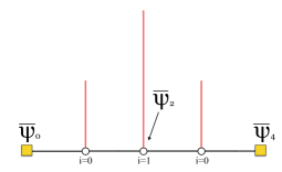
Figure 2: Last three RG-steps $k=l-3$, $l-2$, and $l-1$, in an ultra-walk with absorbing walls (yellow squares). Note that for each RG-step $k\to k+1$, the remaining hierarchy indices $i$ for sites $x$ go from $i\to i-1$, as reflected in Eq. (18). Then, for all sites $x^{(k)}\to x^{(k+1)}=\frac{x^{(k)}}{2}$. The final step $k=l-1\to l$ is described by Eqs. (20-21), assuming that the walk started at the central site, $x=x^{(0)}=2^{l-1}=\frac{N-1}{2}$ in a finite system of size $N=2^{l}+1$, originally, i.e., at $x^{(l-1)}=1$.

III.1 Absorbing walls

While the spreading behavior in itself, characterized by the walk dimension $d_{w}$, is the most fundamental property of a walk, other physical properties may be of interest. Another interesting physical quantity is the absorption of a walk at a wall, classically Boettcher (1995); Boettcher and Moshe (1995); Bender et al. (1995) or quantum Ambainis et al. (2001). In particular, since the spreading behavior merely measures the dynamics of that part of the walk which actually moves, determining the absorption of the walk at a confining wall distant from the initial site provides information about how much of the weight of the walk ever reaches the wall. In turn, if that absorption does not become unity, some weight must have become localized within a bounded domain within those walls. For classical diffusion in a simply connected domain that would seem unphysical. However, QW do exhibit such localization behavior, even in the absence of disorder Inui et al. (2005); Schreiber et al. (2011); Falkner and Boettcher (2014); Vakulchyk et al. (2017); Mareš et al. (2019). Of course, absorption is merely an indirect measure of localization, yet, sufficient to ascertain the lack of it.

As a specific situation for such a setting, it is most convenient within the formalism we have developed to consider a walk between two absorbing walls of separation $N=2^{l}+1$, equidistant from the starting site $x_{0}=2^{l-1}$, as illustrated in Fig. 2. Note that in this $1d$ geometry, these walls completely confine the walk. As the wall-sites $x=0$ and $x=2^{l}$ are fully absorbing, there is no flow out of those sites and at the end of $l-1$ RG-steps the Eqs. (16) reduce to

$$\overline{\psi}_{0} = A_{0}^{(l-1)}\overline{\psi}_{1},$$

$$\overline{\psi}_{1} = M_{0}^{(l-1)}\overline{\psi}_{1}+\psi_{IC},$$ (20)

$$\overline{\psi}_{2} = B_{0}^{(l-1)}\overline{\psi}_{1}.$$

Thus, for either wall it is

$$\overline{\psi}_{\left\{0,2\right\}}=S_{l-1}^{\left\{A,B\right\}}\left({\cal C}_{l-1}^{-1}-S_{l-1}^{M}\right)^{-1}\psi_{IC}.$$ (21)

We will discuss below the RG-prediction for the absorption for both, RW and QW.

IV Solution of the Classical Ultra-Walk

Like for QW, we will find that the state variable describing PRW is now a 2-component vector $\psi_{x,t}$, which here expresses a memory of the previous step. The physics of classical walks with such memory (“persistence”) has been widely studied Weiss (1994); Chen and Renshaw (1994). Based on its prior behavior, the upper component $\psi_{x,t}^{+}$ refers to a walker with the preference to step to the right in the next time-step, and the lower component $\psi_{x,t}^{-}$ indicates a left-hop preference. The value of each component describes the probability of finding a walker at that site $x$ and time $t$ in state “$\pm$”, and the total probability of finding a walker there, irrespective of preference, is simply the sum of the two, $\rho_{x,t}=\psi_{x,t}^{+}+\psi_{x,t}^{-}$. Ignoring a potential left-right bias here, we consider a walker coming from the left (right) to have a probability $\eta_{x}$ to continue to move right (left), and a probability $1-\eta_{x}$ to reverse direction in the next step. For $\eta_{x}>\frac{1}{2}$ ($\eta_{x}<\frac{1}{2}$) the walker exhibits (anti-)persistence, and for $\eta_{x}=\frac{1}{2}$ reduces again to an ordinary unbiased RW without memory. The master equations then reads:

$$\overline{\psi}_{x}^{+} = z\eta_{x}\overline{\psi}_{x-1}^{+}+z\left(1-\eta_{x}\right)\overline{\psi}_{x-1}^{-}+\delta_{x,x_{0}}\overline{\psi}_{IC}^{+},$$

$$\overline{\psi}_{x}^{-} = z\left(1-\eta_{x}\right)\overline{\psi}_{x+1}^{+}+z\eta_{x}\overline{\psi}_{x+1}^{-}+\delta_{x,x_{0}}\overline{\psi}_{IC}^{-},$$ (22)

where $\overline{\psi}_{IC}$ (with $\overline{\psi}_{IC}^{+}+\overline{\psi}_{IC}^{-}=1$) represents the IC of PRW, which we place again at some site $x_{0}$. Thus, $\overline{\psi}_{x}^{+}$ ($\overline{\psi}_{x}^{-}$) only depends on hops from its left (right) neighbor; it is that inflow which induces the “$+$” (“$-$”) state. We can then write Eq. (22) conveniently in matrix notation as a propagator like Eq. (5) with Boettcher et al. (2013)

$$A_{x}=\left(\begin{array}[]{cc}\eta_{x}&1-\eta_{x}\\ 0&0\end{array}\right),\qquad B_{x}=\left(\begin{array}[]{cc}0&0\\ 1-\eta_{x}&\eta_{x}\end{array}\right),$$ (23)

and $M_{x}=0$. As for QW, we can decompose these matrices further to write them as a combination of a shift and a coin matrix, $\{A,B,M\}_{x}=S^{\{A,B,M\}}{\cal C}_{x}$, with the same shift matrices as in Eq. (10). However, here we introduce the stochastic coin matrix

$${\cal C}_{x}=\left(\begin{array}[]{cc}\eta_{x}&1-\eta_{x}\\ 1-\eta_{x}&\eta_{x}\end{array}\right),$$ (24)

in which each row sums to unity.

IV.1 Ultradiffusion as hierarchically anti-persistent walk

With the same choice of a hierarchically defined coin as in Sec. III, decomposing $x=x(i,j)$, PRW is renormalized exactly the same way such as to obtain Eq. (III). [Note that ${\cal C}_{x}$ in Eq. (24) also has an inverse, except for $\eta_{x}=\frac{1}{2}$, the degenerate case of an ordinary (non-persistent) walk, which we can safely exclude in the following.] Then, it is easy to formulate a simple PRW that is in the same universality class as the ultradiffusion model solved in Ref. Maritan and Stella (1986), by choosing for $0\leq\epsilon\leq 1$ and some $\eta_{0}(<\frac{1}{2}$, to ensure invertibility of all coins):

$$\eta_{x(i,j)}=\eta_{i}=\eta_{0}\epsilon^{i}.$$ (25)

For $\epsilon=1$, we expect to recover the ordinary PRW on a homogeneous 1d lattice. Since $\eta_{i}<\frac{1}{2}$ and, indeed, rapidly approaches zero, the walk is increasingly anti-persistent, i.e., ever-larger domains form that are bordered by sites $x$ of high hierarchical index $i$, frustrating the walk attempting to leave the domain with an exponentially smaller probability (or higher barriers) with $i$.

Because the RG recursions in Eq. (III) is expressed in terms of matrices, we need to find a parametrization of those recurring shift-matrices in terms of scalar variables Boettcher et al. (2013). After several iterations of Eq. (III), starting from the unrenormalized shift matrices in Eq. (10), a pattern soon appears that can be parametrized as

$$S_{k}^{A}=\left(\begin{array}[]{cc}a_{k}&0\\ 0&0\end{array}\right),\,S_{k}^{B}=\left(\begin{array}[]{cc}0&0\\ 0&a_{k}\end{array}\right),\,S_{k}^{M}=\left(\begin{array}[]{cc}0&m_{k}\\ m_{k}&0\end{array}\right).$$ (26)

That pattern reproduces itself after a single iteration of Eq. (III) by replacing $k$ with $k+1$ and identifying

$$a_{k+1} = \frac{\eta_{k}a_{k}^{2}}{\left(1-m_{k}\right)\left[1-(1-2\eta_{k})m_{k}\right]},$$ (27)

$$m_{k+1} = m_{k}+\frac{a_{k}^{2}\left[1-\eta_{k}-\left(1-2\eta_{k}\right)m_{k}\right]}{\left(1-m_{k}\right)\left[1-(1-2\eta_{k})m_{k}\right]},$$

as the RG flow, with initial conditions $a_{0}=z$ and $m_{0}=0$. Note that this recursion is non-autonomous due to the explicit $k$-dependence via $\eta_{k}$. We could supplement $\eta_{k}$ as a dynamical variable via its recursion $\eta_{k+1}=\epsilon\eta_{k}$ Maritan and Stella (1986) and study fixed points of those three recursions. However, there is a more elegant approach using the transformations

$$a_{k} = \frac{\eta_{k}}{1-2\eta_{k}}\alpha_{k},$$ (28)

$$m_{k} = \frac{1-\eta_{k}}{1-2\eta_{k}}-\frac{\eta_{k}}{1-2\eta_{k}}\mu_{k},$$

which turn Eqs. (27) into

$$\alpha_{k+1} = \frac{1}{\epsilon}\,\frac{\alpha_{k}^{2}}{\mu_{k}^{2}-1},$$ (29)

$$\mu_{k+1} = \left(1-\frac{1}{\epsilon}\right)+\frac{1}{\epsilon}\mu_{k}\left(1-\frac{\alpha_{k}^{2}}{\mu_{k}^{2}-1}\right),$$

where we have assumed $\frac{\eta_{k}\left(1-2\eta_{k+1}\right)}{\eta_{k+1}\left(1-2\eta_{k}\right)}\sim\frac{1}{\epsilon}$ and $\frac{1-\eta_{k+1}}{\eta_{k+1}}-\frac{\left(1-\eta_{k}\right)\left(1-2\eta_{k+1}\right)}{\eta_{k+1}\left(1-2\eta_{k}\right)}\sim 1-\frac{1}{\epsilon}$, which is justified for $\eta_{k}$ in Eq. (25) at large $k$ for $\epsilon<1$, but trivially holds for the homogeneous walk at $\epsilon=1$ also. Now, the RG-flow in Eq. (29) is purely autonomous but depends non-trivially on the parameter $\epsilon$ that characterizes the strength of the ultrametric barriers. This flow has two obvious fixed points, at $\alpha_{\infty}=\frac{1}{\epsilon}-2$ and $\mu_{\infty}=\frac{1}{\epsilon}-1$, and at $\alpha_{\infty}=\frac{1}{\epsilon}-\epsilon$ and $\mu_{\infty}=-\frac{1}{\epsilon}$. The second one can not be reached by any physical initial condition of the flow, as $\mu_{\infty}<0$. The first fixed point is physical for $0\leq\epsilon\leq\frac{1}{2}$, where the largest eigenvalue of the Jacobian of the flow in Eq. (29) is $\lambda=\frac{2}{\epsilon}$, which reproduces the anomalous walk dimension,

$$d_{w}=1-\log_{2}\epsilon,$$ (30)

found in Ref. Maritan and Stella (1986). When $\epsilon\to\frac{1}{2}$, $d_{w}\to 2$ and the effect of the barriers becomes irrelevant such that ordinary diffusion ensues for all $\frac{1}{2}\leq\epsilon\leq 1$, making diffusion rather robust against the introduction of such a set of barriers. [In fact, for $\epsilon=1$ only, we can find a closed form solution for all $k$ of the RG-flow in Eq. (29), as in Refs. Boettcher and Li (2018, 2015).] However, to find the fixed point for the diffusive solutions for $\frac{1}{2}\leq\epsilon\leq 1$ requires a scaling ansatz with $\alpha_{k}=\left(2\epsilon\right)^{-k}x_{k}$ and $\mu_{k}=1+\left(2\epsilon\right)^{-k}y_{k}$ such that

$$x_{k+1}\sim\frac{x_{k}^{2}}{y_{k}}, y_{k+1}\sim 2y_{k}-\frac{x_{k}^{2}}{y_{k}},$$ (31)

now independent of $\epsilon$, with fixed point $x_{\infty}=y_{\infty}$ and a Jacobian eigenvalue of $\lambda=4$, i.e., $d_{w}=2$. These results are summarized in Fig. 3.

Finally, we note that replacing the anti-persistent hierarchy of coins with a persistent one, easily achieved by replacing $\eta_{x}\to 1-\eta_{x}$ in Eq. (24), leads again to a purely diffusive walk for all $\epsilon$. The asymptotic analysis for large $k$ with $\epsilon^{k}\to 0$ now yields the $\epsilon\to 1$ limit of Eq. (29) even for $\epsilon<1$ that then results in Eq. (31) with $d_{w}=2$. It is easy to see that the physical situation of a persistent hierarchy differs dramatically from the anti-persistent one: For large $k$, all coins now become transmissive (i.e., the identity matrix) instead of reflective, leaving mostly the non-diagonal coins at all odd sites ($i=0$) to institute a simple persistent, and effectively homogeneous, walk that remains in the same universality class as ordinary diffusion Weiss (1994).

IV.2 Classical walk with absorbing walls

Evaluation of Eq. (21) for the geometry of Fig. 2 using the coin in Eq. (24) and the RG parametrization in Eq. (26) after $k=l$ RG-steps, then taking $l\to\infty$, we readily obtain

$$\overline{\psi}_{\left\{0,2\right\}} = \frac{\alpha_{\infty}}{\mu_{\infty}^{2}-1}S^{\left\{A,B\right\}}\left(\begin{array}[]{cc}1&\mu_{\infty}\\ \mu_{\infty}&1\end{array}\right)\psi_{IC},$$ (34)

$$= S^{\left\{A,B\right\}}\left(\begin{array}[]{cc}\epsilon&1-\epsilon\\ 1-\epsilon&\epsilon\end{array}\right)\psi_{IC},$$ (37)

with $S^{\left\{A,B\right\}}$ given in Eq. (10). In PRW, the norm of a state-vector is simply the sum of its (certainly non-negative) components, $\left\|\psi_{x,t}\right\|\stackrel{{\scriptstyle def}}{{=}}\left(\begin{array}[]{c}1\\ 1\end{array}\right)\circ\psi_{x,t}$. Then, for an absorbing site $x$, the absorption there is $F_{x}=\sum_{t=0}^{\infty}\left|\psi_{x,t}\right|=\left\|\overline{\psi}_{x}\left(z=1\right)\right\|$. With $S^{A}+S^{B}=\mathbb{I}$, we finally get for the total (combined) absorption:

$$F_{0+2}=\left\|\overline{\psi}_{0}+\overline{\psi}_{2}\right\|=\left\|\psi_{IC}\right\|=1,$$ (38)

since $\psi_{IC}$ is normed to unity, of course. Thus, for any size barrier $\epsilon$ and any system size, any walk started in the middle will eventually get absorbed with certainty! For a classical walk on the 1d-line, we would have expected this, due to Polya’s theorem Pólya (1921), even for a heterogeneous environment.

V Solution of the Quantum Ultra-Walk

To design a quantum analogue to the classical PRW on an ultrametric set of barriers, specified by Eq. (24), we consider the real, unitary quantum coins

$${\cal C}_{i}=\left(\begin{array}[]{cc}\sin\eta_{i}&\cos\eta_{i}\\ \cos\eta_{i}&-\sin\eta_{i}\end{array}\right),\qquad\eta_{i}=\eta_{0}\epsilon^{i}\quad(0<\epsilon\leq 1),$$ (39)

although many other interesting choices may exist Vakulchyk et al. (2017). Note that for $\epsilon=1$, this reproduces a homogeneous 1d QW Boettcher et al. (2013). However, for $\epsilon<1$, the coins become increasingly resistant to transit, with $\eta_{i}\to 0$ for $i\to\infty$, blocking the transition through sites $x$ of higher index $i$, no matter from which direction those sites are approached.

As for the classical case, evolving the recursions in Eq. (III) with this coin for a few iterations from the unrenormalized values, already after one iteration a recurring pattern emerges that suggest the Ansatz

$$S_{k}^{A}=\left(\begin{array}[]{cc}a_{k}&0\\ 0&0\end{array}\right),\,S_{k}^{B}=\left(\begin{array}[]{cc}0&0\\ 0&-a_{k}\end{array}\right),\,S_{k}^{M}=\left(\begin{array}[]{cc}0&m_{k}\\ m_{k}&0\end{array}\right),$$ (40)

amazingly similar to the classical case in Eq. (26). When iterated, the RG-recursions in Eq. (III) for the scalar parametrization with $a_{k}$ and $m_{k}$ closes after each iteration for

$$a_{k+1} = \frac{a_{k}^{2}\sin\eta_{k}}{1-2m_{k}\cos\eta_{k}+m_{k}^{2}},$$ (41)

$$m_{k+1} = m_{k}+\frac{\left(m_{k}-\cos\eta_{k}\right)a_{k}^{2}}{1-2m_{k}\cos\eta_{k}+m_{k}^{2}},$$

with $a_{k=1}=z^{2}\sin\eta_{0}$, $m_{k=1}=z^{2}\cos\eta_{0}$, and $\eta_{1}=\eta_{0}\epsilon$ as initial conditions. [Only the first step, from $k=0$ to $k=1$, does not fit this pattern.] Note the striking similarity of these recursions to those for PRW in PRW in Eq. (27). Like those, Eq. (41) is non-autonomous. Analogous to Eq. (28), we can find an elegant transformation,

$$a_{k}=\alpha_{k}\sin\eta_{k}, m_{k}=\cos\eta_{k}-\mu_{k}\sin\eta_{k},$$ (42)

that turns Eq. (41) into

$$\alpha_{k+1} \sim \frac{1}{\epsilon}\,\frac{\alpha_{k}^{2}}{\mu_{k}^{2}+1},$$ (43)

$$\mu_{k+1} \sim \frac{1}{\epsilon}\,\mu_{k}\,\left(1+\frac{\alpha_{k}^{2}}{\mu_{k}^{2}+1}\right)+\frac{1}{2}\eta_{k}\left(\epsilon-\frac{1}{\epsilon}\right),$$

where we have approximated $\frac{\sin\eta_{k+1}}{\sin\eta_{k}}\sim\epsilon$ and $\left(\cos\eta_{k}-\cos\eta_{k+1}\right)/\sin\eta_{k+1}\sim\frac{1}{2}\eta_{k}\left(\epsilon-1/\epsilon\right)$, to within exponentially small corrections in $k$ for $\epsilon<1$, and trivially correct for $\epsilon=1$.

If we were to consider neglecting the last term in Eq. (43), that is exponentially small for $\epsilon<1$, we find a fixed point at $\alpha_{\infty}=1-\frac{1}{\epsilon}$ and $\mu_{\infty}=\pm i\sqrt{1-\frac{1}{\epsilon}+\frac{1}{\epsilon^{2}}}$. Having $\alpha_{\infty}<0$ imposes no restriction, since the definition of $a_{k}$ in Eq. (40) is invariant under $a_{k}\to-a_{k}$. Having imaginary $\mu_{\infty}$ could be expected as a small correction off the real axis to $m_{\infty}=1$ in a quantum problem. The associated eigenvalues are very interesting, with

$$\lambda_{\pm} = \left(\frac{1}{\epsilon}+\frac{1}{2}+\epsilon\right)\pm\sqrt{\left(\frac{1}{\epsilon}+\frac{1}{2}+\epsilon\right)^{2}-2},$$ (44)

of which only $\lambda_{+}>1$ for $0<\epsilon<1$. In fact, it reproduces the eigenvalues found for a corresponding tight-binding spectrum considered in Ref. Ceccatto et al. (1987). As shown in Fig. 3, it meets up with the classical result for $d_{w}$ really well for $\epsilon\to 0$. However, it generally predicts a slower spread than even the classical walk throughout. Closer inspection of the boundary layer Bender and Orszag (1978) at $\epsilon\to 1$ shows that it is actually a very subtle extension of the (subdominant) diffusive solution found for the ordinary 1d QW discussed in Ref. Boettcher et al. (2013). While $\lambda_{+}\to\left(5+\sqrt{17}\right)/2\approx 4.56...$ for $\epsilon\to 1$, this fixed point is actually not valid for $\epsilon=1$, since $\mu_{\infty}\to\pm i$ and $\alpha_{\infty}\to 0$, for which the recursions in Eq. (43) are singular. Resolving that singularity with a scaling ansatz reproduces the diffusive solution with $\lambda=4$ to which $\lambda_{+}$ discontinuously connects.

To reveal the physically relevant scaling of QW, we argue as follows: Without the last term in Eq. (43), there is also a fixed point values of $\alpha_{\infty}=\epsilon$ and $\mu_{\infty}=0$, which in turn is inconsistent with dropping even an exponentially small term, however. Rather, we retain the term and apply the Ansatz $\mu_{k}=\eta_{k}\nu_{k}\ll 1$ with $\nu_{k}$ finite to turn all of Eq. (43) autonomous:

$$\alpha_{k+1} \sim \frac{\alpha_{k}^{2}}{\epsilon},$$ (45)

$$\nu_{k+1} \sim \frac{\nu_{k}}{\epsilon^{2}}\,\left(1+\alpha_{k}^{2}\right)-\frac{1-\epsilon^{2}}{2\epsilon^{2}},$$

The flow in Eq. (45) has a fixed point at $\alpha_{\infty}=\epsilon$ and $\nu_{\infty}=\frac{1}{2}\left(1-\epsilon^{2}\right)$. Its Jacobian eigenvalues are $\lambda_{1}=1+\epsilon^{-2}$ and $\lambda_{2}=2$, i.e., $\lambda_{1}\geq\lambda_{2}>1$ for $0\leq\epsilon\leq 1$. For a classical walk with a stochastic master equation, the leading eigenvalue $\lambda_{1}$ suffices to describe the walk dimension $d_{w}=\log_{2}\lambda_{1}$ Redner (2001). However, it has been shown Boettcher et al. (2017); Boettcher and Li (2018) that the unitarity constraint imposed on the master equation for QW also requires physical observables to be unitary. . Yet, the renormalized parameters $a_{k}$ and $m_{k}$ are not, and their poles move with $k$ both, tangentially and radially, to the unit circle in the complex $z$-plane, while the poles of actual observables only move tangentially on the circle, see Eq. (3). Detailed analysis shows Boettcher et al. (2017) that the largest,dominant eigenvalue, $\lambda_{1},$ only describes the tangential movement of poles and, thus, must be ignored . Instead, the tangential movement of poles is found to be described by the geometric mean of first and second eigenvalue, $\sqrt{\lambda_{1}\lambda_{2}}$. Accordingly, we conclude that

$$d_{w}^{Q}=\log_{2}\sqrt{\lambda_{1}\lambda_{2}}=\frac{1}{2}+\frac{1}{2}\log_{2}\left(1+\epsilon^{-2}\right).$$ (46)

This walk dimension, also shown in Fig. 3, has all the characteristics of being physical, as it is ballistic ($d_{w}=1$) for the homogeneous 1d QW at $\epsilon\to 1$, and it diverges for diverging barrier heights, $\epsilon\to 0$, where to leading order matches up with the classical result, $d_{w}\sim-\log_{2}\epsilon$. It also predicts the fastest spread for QW compared to RW or the fixed point leading to Eq. (44). Note also that even a minute disturbance of homogeneity, i.e., barriers for arbitrarily small $1-\epsilon$, QW ceases to be ballistic.

While it is easy to simulate QW for any $\epsilon$, it remains a challenge to interpret the data, in particular, to test Eq. (46). Unlike for RW, the deterministic, unitary evolution of QW does not provide for much of a stochastic variation over which repeated walks could be averaged. Additionally, sometimes dramatic changes in the behavior of a walk occur especially near large barriers. Both of these effects are on display in Fig. 4, showing the PDF of QW with $\epsilon=\frac{1}{2}$, re-scaled according to Eq. (4). Large spatial fluctuations, and ever more pronounced jumps near larger barriers, make it difficult to collapse the data with any accuracy. However, asymptotically such a collapse with $d_{w}=1.661$, as Eq. (46) provides, seems plausible.

Figure 3: Plot of the inverse walk dimension $1/d_{w}$ for the classical (RW) and the quantum walk (QW) with ultrametric barriers as a function of coin-parameter $\epsilon$, where smaller $\epsilon$ represents higher barriers between an ultrametrically arrange hierarchy of domains that confine the walk. The black and the blue lines are the respective RG-predictions in Eq. (30) and in Eq. (46). Also, the unphysical prediction from the eigenvalue $\lambda_{+}$ in Eq. (44) is shown as red-dashed line.

Figure 4: Plot of the PDF $\rho(x,t)$ as a function of pseudo-velocity $x/t^{1/d_{w}}$, see Eq. (4), for a range of times $t$ after the initiation of the walk at $x=0$. (Only $x\geq 0$ is shown.) In these simulations, we set $\epsilon=\frac{1}{2}$ so that $d_{w}=1.661$, according to Eq. (46).

V.1 Quantum walk with absorbing walls

Unlike for the classical case discussed in Sec. IV.2, where the total absorption amounts conveniently to taking a local limit for $z\to 1$ on the Laplace transform of the site amplitude, evaluating the adsorption in QW is surprisingly involved, in comparison. Due to unitarity, the adsorption sums up the square modulus of site amplitudes, which correspond to contour integrals over the entire unit circle in the complex $z-$plane for the modulus of their Laplace transforms,

$$F_{0}=\sum_{t=0}^{\infty}\left|\psi_{0,t}\right|^{2}=\oint\frac{dz}{2\pi iz}\left|\overline{\psi}_{0}\left(z\right)\right|^{2},$$ (47)

Such an integral is readily, albeit strenuously, evaluated for the simple case of homogeneous QW ($\epsilon=1$), using the non-linear Riemann-Lebesgue lemma Ambainis et al. (2001). However, for $\epsilon<1$ we have only the local asymptotic evaluation of the RG recursions in Eq. (41) available. While, for instance, $\overline{\psi}_{0}\left(z\right)$ in Eq. (47) is a functional of the hopping operators, inserting their asymptotic form for a local expansion of the integral does not appear to be sufficient to obtain the absorption.

As mentioned above, resorting instead to a direct simulation of QW shows that it is difficult to extract the scaling for moments of the walk to, say, verify the walk dimension in Eq. (46) with any reasonable accuracy. The irregular pattern of reflecting barriers leads to very noisy probability densities. However, it is quite easy to convince oneself, starting from very small systems and progressively doubling their size, that the total absorption remains exactly unity throughout for even the smallest values of $\epsilon$. Thus, there appears to be no localization in the interior of the system; all of the weight of QW eventually reaches a wall!

VI Conclusions

The ultra-walk provides an exactly solvable model of a walk, both classical or quantum, with tunable spatial heterogeneity. For the classical case, we reproduce previous results by alternative means, using a $2^{{\rm nd}}-$order Markov process that closely resembles the coined QW in form. For the discrete-time QW, we obtain entirely new results over the entire range of heterogeneity, with walk dimensions ranging from $d_{w}^{QW}=1$ to infinity. Thus, while RW is quite robust against the introduction of those barriers, even the smallest amount of inhomogeneity changes the asymptotic behavior of QW. However, numerical verification of these results for QW is difficult to obtain, due to the strong hierarchical nature. Focusing on the absorption problem at walls that recede from the starting site with increasing system size, we can at least ascertain, as in the classical case, that there is no localization, even for the most extreme heterogeneity. Future work will focus on the asymptotic evaluation of observables, like the absorption in Eq. (47), that are defined via a complex integration for QW. Absorption, transit and first passage problems of that sort are fundamental to any transport problem, classical or quantum Kampen (1992); Redner (2001).

Acknowledgments:

SB acknowledges financial support during the preparation of this manuscript from the U. S. National Science Foundation through grant DMR-1207431 and from CNPq through the “Ciência sem Fronteiras” program, and he thanks Renato Portugal, Stefan Falkner, and Shanshan Li for many helpful discussions and LNCC for its hospitality.

References

- Portugal (2013) R. Portugal, Quantum Walks and Search Algorithms (Springer, Berlin, 2013).
- Grover (1997) L. K. Grover, Phys. Rev. Lett. 79, 325 (1997).
- Shenvi et al. (2003) N. Shenvi, J. Kempe, and K. Whaley, Phys. Rev. A 67, 052307 (2003).
- Ambainis et al. (2005) A. Ambainis, J. Kempe, and A. Rivosh, in Proceedings of the sixteenth annual ACM-SIAM symposium on Discrete algorithms, SODA ’05 (Society for Industrial and Applied Mathematics, Philadelphia, PA, USA, 2005) 1099–1108.
- Boettcher et al. (2018) S. Boettcher, S. Li, T. D. Fernandes, and R. Portugal, Physical Review A 98, 012320 (2018).
- Childs and Goldstone (2004) A. M. Childs and J. Goldstone, Phys. Rev. A 70, 022314 (2004).
- Kempe (2003) J. Kempe, Contemporary Physics 44, 307 (2003).
- Venegas-Andraca (2012) E. Venegas-Andraca, Quantum Information Processing 11, 1015 (2012).
- Ambainis et al. (2001) A. Ambainis, E. Bach, A. Nayak, A. Vishwanath, and J. Watrous, Annual ACM Symposium on Theory of Computing 33, 37 (2001).
- Konno (2002) N. Konno, Quantum Information Processing 1, 345 (2002).
- Inui et al. (2004) N. Inui, Y. Konishi, and N. Konno, Physical Review A 69, 052323 (2004).
- Bach et al. (2004) E. Bach, S. Coppersmith, M. P. Goldschen, R. Joynt, and J. Watrous, Journal of Computer and System Sciences 69, 562 (2004).
- Inui et al. (2005) N. Inui, N. Konno, and E. Segawa, Phys. Rev. E 72, 056112 (2005).
- Mackay et al. (2002) T. D. Mackay, S. D. Bartlett, L. T. Stephenson, and B. C. Sanders, J. Phys. A: Math. Gen. 35, 2745 (2002).
- Marquezino et al. (2013) F. L. Marquezino, R. Portugal, and S. Boettcher, Phys. Rev. A 87, 012329 (2013).
- Patel and Raghunathan (2012) A. Patel and K. S. Raghunathan, Phys. Rev. A 86, 012332 (2012).
- Boettcher et al. (2015) S. Boettcher, S. Falkner, and R. Portugal, Phys. Rev. A 91, 052330 (2015).
- Marquezino et al. (2007) F. L. Marquezino, R. Portugal, G. Abal, and R. Donangelo, Physical Review A 77, 042312 (2007), 0712.0625 .
- Konno (2005) N. Konno, J. Math. Soc. Japan 57, 1179 (2005).
- Schreiber et al. (2011) A. Schreiber, K. N. Cassemiro, V. Potoček, A. Gábris, I. Jex, and C. Silberhorn, Phys. Rev. Lett. 106, 180403 (2011).
- Falkner and Boettcher (2014) S. Falkner and S. Boettcher, Phys. Rev. A 90, 012307 (2014).
- Vakulchyk et al. (2017) I. Vakulchyk, M. V. Fistul, P. Qin, and S. Flach, Physical Review B 96, 144204 (2017).
- Mareš et al. (2019) J. Mareš, J. Novotný, and I. Jex, Physical Review A 99, 042129 (2019).
- Perets et al. (2008) H. B. Perets, Y. Lahini, F. Pozzi, M. Sorel, R. Morandotti, and Y. Silberberg, Phys. Rev. Lett. 100, 170506 (2008).
- Peruzzo et al. (2010) A. Peruzzo, M. Lobino, J. C. F. Matthews, N. Matsuda, A. Politi, K. Poulios, X.-Q. Zhou, Y. Lahini, N. Ismail, K. Wörhoff, Y. Bromberg, Y. Silberberg, M. G. Thompson, and J. L. OBrien, Science 329, 1500 (2010).
- Schreiber et al. (2012) A. Schreiber, A. Gábris, P. P. Rohde, K. Laiho, M. Štefaňák, V. Potoček, C. Hamilton, I. Jex, and C. Silberhorn, Science 336, 55 (2012).
- Sansoni et al. (2012) L. Sansoni, F. Sciarrino, G. Vallone, P. Mataloni, A. Crespi, R. Ramponi, and R. Osellame, Phys. Rev. Lett. 108, 010502 (2012).
- Crespi et al. (2013) A. Crespi, R. Osellame, R. Ramponi, V. Giovannetti, R. Fazio, L. Sansoni, F. D. Nicola, F. Sciarrino, and P. Mataloni, Nature Photonics 7, 322 (2013).
- Qiang et al. (2016) X. Qiang, T. Loke, A. Montanaro, K. Aungskunsiri, X. Zhou, J. L. O’Brien, J. B. Wang, and J. C. F. Matthews, Nature Communications 7, 11511 (2016).
- Ramasesh et al. (2017) V. V. Ramasesh, E. Flurin, M. Rudner, I. Siddiqi, and N. Y. Yao, Phys. Rev. Lett. 118, 130501 (2017).
- Figgatt et al. (2017) C. Figgatt, D. Maslov, K. A. Landsman, N. M. Linke, S. Debnath, and C. Monroe, Nature Communications 8, 1918 (2017).
- Foulger et al. (2014) I. Foulger, S. Gnutzmann, and G. Tanner, Phys. Rev. Lett. 112, 070504 (2014).
- Tang et al. (2018a) H. Tang, C. D. Franco, Z.-Y. Shi, T.-S. He, Z. Feng, J. Gao, K. Sun, Z.-M. Li, Z.-Q. Jiao, T.-Y. Wang, M. S. Kim, and X.-M. Jin, Nature Photonics 12, 754 (2018a).
- Tang et al. (2018b) H. Tang, X.-F. Lin, Z. Feng, J.-Y. Chen, J. Gao, K. Sun, C.-Y. Wang, P.-C. Lai, X.-Y. Xu, Y. Wang, L.-F. Qiao, A.-L. Yang, and X.-M. Jin, Science Advances 4, 3174 (2018b).
- Shikano and Katsura (2010) Y. Shikano and H. Katsura, Phys. Rev. E 82, 031122 (2010).
- Ogielski and Stein (1985) A. T. Ogielski and D. L. Stein, Phys. Rev. Lett. 55, 1634 (1985).
- Huberman and Kerszberg (1985) B. Huberman and M. Kerszberg, J.Phys.A 18, L331 (1985).
- Maritan and Stella (1986) A. Maritan and A. Stella, J. Phys A: Math. Gen. 19, L269 (1986).
- Sibani (1986) P. Sibani, Phys. Rev. B 34, 3555 (1986).
- Ceccatto et al. (1987) H. A. Ceccatto, W. P. Keirstead, and B. A. Huberman, Phys. Rev. A 36, 5509 (1987).
- Hoffmann and Sibani (1988) K. H. Hoffmann and P. Sibani, Phys. Rev. A 38, 4261 (1988).
- Pathria (1996) R. K. Pathria, Statistical Mechanics, 2nd Ed. (Butterworth-Heinemann, Boston, 1996).
- Itzykson and Drouffe (1989) C. Itzykson and J.-M. Drouffe, Statistical Field Theory (Cambridge University Press, 1989).
- Pólya (1921) G. Pólya, Mathematische Annalen 84, 149 (1921).
- Boettcher and Li (2018) S. Boettcher and S. Li, Physical Review A 97, 012309 (2018).
- Chen and Renshaw (1994) A. Chen and E. Renshaw, Journal of Applied Probability 31, 869 (1994).
- Weiss (1994) G. H. Weiss, Aspects and Applications of the Random Walk (North-Holland, Amsterdam, 1994).
- Boettcher et al. (2013) S. Boettcher, S. Falkner, and R. Portugal, Journal of Physics: Conference Series 473, 012018 (2013).
- Redner (2001) S. Redner, A Guide to First-Passage Processes (Cambridge University Press, Cambridge, 2001).
- Boettcher et al. (2017) S. Boettcher, S. Li, and R. Portugal, J. Phys. A 50, 125302 (2017).
- Havlin and Ben-Avraham (1987) S. Havlin and D. Ben-Avraham, Adv. Phys. 36, 695 (1987).
- Feller (1966) W. Feller, An Introduction to Probability Theory and its Applications, vol. I (John Wiley, New York London Sidney Toronto, 1966).
- Bouchaud and Georges (1990) J.-P. Bouchaud and A. Georges, Phys. Rep. 195, 127 (1990).
- Grimmett et al. (2004) G. Grimmett, S. Janson, and P. F. Scudo, Physical Review E 69, 026119 (2004).
- Segawa and Konno (2008) E. Segawa and N. Konno, Int. J. Quant. Inform. 6, 1231 (2008).
- Konno (2008) N. Konno, in Quantum Potential Theory, Lecture Notes in Mathematics, Vol. 1954, edited by U. Franz and M. Schürmann (Springer-Verlag: Heidelberg, Germany, 2008) 309–452.
- Boettcher et al. (2014) S. Boettcher, S. Falkner, and R. Portugal, Phys. Rev. A 90, 032324 (2014).
- Hughes (1996) B. D. Hughes, Random Walks and Random Environments (Oxford University Press, Oxford, 1996).
- Note (1) We assume that both, the unitary but also the stochastic coin, have an inverse.
- Boettcher (1995) S. Boettcher, Phys. Rev. E 51, 3862 (1995).
- Boettcher and Moshe (1995) S. Boettcher and M. Moshe, Phys. Rev. Lett. 74, 2410 (1995).
- Bender et al. (1995) C. M. Bender, S. Boettcher, and P. N. Meisinger, Phys. Rev. Lett. 75, 3210 (1995).
- Boettcher and Li (2015) S. Boettcher and S. Li, J. Phys. A 48, 415001 (2015).
- Bender and Orszag (1978) C. M. Bender and S. A. Orszag, Advanced Mathematical Methods for Scientists and Engineers (McGraw-Hill, New York, 1978).
- Note (2) In the appendix of Ref. Boettcher et al. (2017) an example was provided that shows by explicit construction how the poles of the non-unitary hopping parameters cancel as soon as these parameters are combined to calculate an observable.
- Kampen (1992) N. G. V. Kampen, Stochastic Processes in Physics and Chemistry (North Holland, Amsterdam, 1992).