Model structures and fitting criteria for system identification with neural networks

Abstract

This paper focuses on the identification of dynamical systems with tailor-made model structures, where neural networks are used to approximate uncertain components and domain knowledge is retained, if available. These model structures are fitted to measured data using different criteria including a computationally efficient approach minimizing a regularized multi-step ahead simulation error. The neural network parameters are estimated along with the initial conditions used to simulate the output signal in small-size subsequences. A regularization term is included in the fitting cost in order to enforce these initial conditions to be consistent with the estimated system dynamics.

  To cite this work, please use the following bibtex entry:

@inproceedings{forgione2020model,
  title={Model structures and fitting criteria for system identification
  with neural networks},
  author={Forgione, Marco and Piga, Dario},
  booktitle={Proc. of the 14th IEEE International Conference Application
  of Information and Communication Technologies, Tashkent, Uzbekistan},
  year={2020}
}

Using the plain bibtex style, the bibliographic entry should look like:

M. Forgione, D. Piga. Model structures and fitting criteria for system identification with neural networks. In Proc. of the 14th IEEE International Conference Application of Information and Communication Technologies, Tashkent, Uzbekistan, 2020.

 

1 Introduction

In recent years, deep learning has advanced at a tremendous pace and is now the core methodology behind cutting-edge technologies such as speech recognition, image classification and captioning, language translation, and autonomous driving [Schmidhuber, 2015]. These impressive achievements are attracting ever increasing investments both from the private and the public sector, fueling further research in this field.

A good deal of the advancement in the deep learning area is of public domain, both in terms of scientific publications and software tools. Nowadays, highly optimized and user-friendly deep learning frameworks are available [Paszke et al., 2017], often distributed under permissive open-source licenses. Using the high-level functionalities of a deep learning framework and following good practice, even a novice user can deal with standard machine learning tasks (once considered extremely hard) such as image classification with moderate effort. Under the hood, the machine learning task is automatically transformed into a relevant optimization problem and subsequently solved through efficient numerical routines.

An experienced practitioner can employ the same deep learning framework at a lower level to tackle non-standard learning problems, by defining customized models and objective functions to be optimized, and using operators such as neural networks as building blocks. The practitioner is free from the burden of writing optimization code from scratch for every particular problem, which would be tedious and error-prone. In fact, as a built-in feature, modern deep learning engines can compute the derivatives of a supplied objective function with respect to free tunable parameters by implementing the celebrated back-propagation algorithm [Rumelhart et al., 1988]. In turn, this enables convenient setup of any gradient-based optimization method.

An exciting, challenging—and yet largely unexplored—application field is system identification with tailor-made model structures and fitting criteria. In this context, neural networks can be used to describe uncertain components of the dynamics, while retaining structural (physical) knowledge, if available. Furthermore, the fitting criterion can be specialized to take into account the modeler’s ultimate goal, which could be prediction, failure detection, state estimation, control design, simulation, etc.

The choice of the cost function may also be influenced by computational considerations. In this paper, in particular, models are evaluated according to their simulation performance. In this setting, from a theoretical perspective, simulation error minimization is generally the best fitting criterion. However, computing the simulation error loss and its derivatives may be prohibitively expensive from a computational perspective for dynamical models involving neural networks. We show that multi-step simulation error minimization over batches of small-size subsequences extracted from the identification dataset provides models with high simulation performance, while keeping the computational burden of the fitting procedure acceptable. In the proposed method, the neural network parameters are jointly estimated with the initial conditions used to simulate the system in each subsequence. A regularization term is also included in the fitting criterion in order to enforce all these initial conditions to be consistent with the estimated system dynamics.

The use of neural networks in system identification has a long history, see, e.g., [Werbos, 1989, Chen et al., 1990]. Even though motivated by similar reasoning, these earlier works are hardly comparable given the huge gap of hardware/software technology. More recently, a few interesting approaches using modern deep learning tools and concepts in system identification have been presented. For instance, [Masti and Bemporad, 2018] introduces a technique to identify neural state-space model structures using deep autoencoders for state reconstruction, while [Gonzalez and Yu, 2018, Wang, 2017] discuss the use of Long Short-Term Memory (LSTM) recurrent neural networks for system identification. Compared to these recent contributions, our work focuses on using specialized model structures for the identification task at hand. In the machine learning community, neural networks have also been recently applied for approximating the solution of ordinary and partial differential equation, see e.g., [Chen et al., 2018, Raissi et al., 2019]. With respect to these contributions, our aim is to find computationally efficient fitting strategies that are robust to the measurement noise.

The rest of this paper is structured as follows. The overall settings and problem statement is outlined in Section 2. The neural dynamical model structures are introduced in Section 3 and criteria for fitting these model structures to training data are described in Section 4. Simulation results are presented in Section 5 and can be replicated using the codes available at https://github.com/forgi86/sysid-neural-structures-fitting. Conclusions and directions for future research are discussed in Section 6.

2 Problem Setting

We are given a dataset ${\mathcal{D}}$ consisting of $N$ input samples $U=\{u_{0},\;u_{1},\dots,\;u_{N-1}\}$ and output samples $Y=\{y_{0},\;y_{1},\dots,\;y_{N-1}\}$, gathered from an experiment on a dynamical system ${S}$. The data-generating system ${S}$ is assumed to have the discrete-time state-space representation

$$x_{k+1} =f(x_{k},u_{k})$$ (1a)

$$y^{\text{o}}_{k} =g(x_{k}),$$ (1b)

where $x_{k}\in\mathbb{R}^{n_{x}}$ is the state at time $k$; $y^{\text{o}}_{k}\in\mathbb{R}^{n_{y}}$ is the noise-free output; $u_{k}\in\mathbb{R}^{n_{u}}$ is the input; $f(\cdot,\cdot)$ and $g(\cdot)$ are the state and output mappings, respectively. The measured output $y_{k}$ is corrupted by a zero-mean noise $\eta_{k}$, i.e., $y_{k}=y^{\text{o}}_{k}+\eta_{k}$.

The aim of the paper is twofold:

• to introduce flexible neural model structures that are suitable to represent generic dynamical systems as (1), allowing the modeler to embed domain knowledge to various degrees and to exploit neural networks’ universal approximation capabilities (see [Hornik et al., 1989]) to describe unknown model components;

• to present robust and computationally efficient procedures to fit these neural model structures to the training dataset ${\mathcal{D}}$.

2.1 Full model structure hypothesis

Let us consider a model structure $\mathcal{M}=\{{M}(\theta),\;\theta\in\mathbb{R}^{n_{\theta}}\}$, where $M(\theta)$ represents a dynamical model parametrized by a real-valued vector $\theta$. We refer to neural model structures as structures $\mathcal{M}$ where some components of the model $M(\theta)$ are described by neural networks.

Throughout the paper, we will make the following full model structure hypothesis: there exists a parameter ${\theta_{\rm o}}\in\mathbb{R}^{n_{\theta}}$ such that the model ${M}({\theta_{\rm o}})\in\mathcal{M}$ is a perfect representation of the true system ${S}$, i.e., for every input sequence, ${M}({\theta_{\rm o}})$ and ${S}$ provide the same output. We denote this condition as ${M}({\theta_{\rm o}})={S}$. Note that the parameter ${\theta_{\rm o}}$ may not be unique. Indeed, deep neural networks have multiple equivalent representations obtained, for instance, by permuting neurons in a hidden layer. Let $\Theta_{S}$ be the set of parameters that provide a perfect system description, namely $\Theta_{S}=\{\theta\in\Theta\text{ such that }{M}(\theta)={S}\}$. Under the full model structure hypothesis, the ultimate identification goal is to find a parameter $\theta\in\Theta_{S}$.

Remark 1

In practice, fitting is performed on a finite-length dataset ${\mathcal{D}}$ covering a finite number of experimental conditions. To this aim, let us introduce the notation ${M}(\theta)\mathrel{\overset{\makebox[0.0pt]{\mbox{\tiny${\mathcal{D}}$}}}{=}}{S}$ meaning that the model ${M}(\theta)$ perfectly matches ${S}$ on the dataset ${\mathcal{D}}$ and let us define the parameter set $\Theta_{S}^{\mathcal{D}}=\{\theta\in\Theta\text{ such that }{M}(\theta)\mathrel{\overset{\makebox[0.0pt]{\mbox{\tiny${\mathcal{D}}$}}}{=}}{S}\}$. By definition, $\Theta_{S}\subseteq\Theta_{S}^{\mathcal{D}}$. Thus, when fitting the model structure to a finite-length dataset ${\mathcal{D}}$, we aim to find a parameter $\theta\in\Theta_{S}^{{\mathcal{D}}}$ (but not necessarily in $\Theta_{{S}}$).

3 Neural model structures

In this section, we introduce possible neural model structures for dynamical systems.

3.1 State-space structures

A general state-space neural model structure has form

$$x_{k+1} =\mathcal{N\!N}_{x}(x_{k},u_{k};\theta)$$ (2a)

$$y^{\rm o} =\mathcal{N\!N}_{y}(x_{k};\theta),$$ (2b)

where $\mathcal{N\!N}_{x}$ and $\mathcal{N\!N}_{y}$ are feedforward neural networks of compatible size parametrized by $\theta\in\mathbb{R}^{n_{\theta}}$. Such a general structure can be tailored for the identification task at hand. Examples are reported in the following paragraphs.

Residual model

If a linear approximation of the system is available, an appropriate model structure is

$$x_{k+1} =A_{L}x_{k}+B_{L}u_{k}+\mathcal{N\!N}_{x}(x_{k},u_{k};\theta),$$ (3a)

$$y_{k} =C_{L}x_{k}+\mathcal{N\!N}_{y}(x_{k},u_{k};\theta),$$ (3b)

where $A_{L}$, $B_{L}$, and $C_{L}$ are matrices of compatible dimensions describing the linear system approximation. Even though model (3) is not more general than (2), it could be easier to train as the neural networks $\mathcal{N\!N}_{x}$ and $\mathcal{N\!N}_{y}$ are supposed to capture only residual (nonlinear) dynamics.

Integral model

When fitting data generated by a continuous-time system, the following neural model with an integral term in the state equation can be used to encourage continuity of the solution:

$$x_{k+1} =x_{k}+\mathcal{N\!N}_{x}(x_{k},u_{k};\theta)$$ (4a)

$$y^{\rm o} =\mathcal{N\!N}_{y}(x_{k},u_{k};\theta).$$ (4b)

This structure can also be interpreted as the forward Euler discretization scheme applied to an underlying continuous-time state-space model.

Fully-observed state model

If the system state is known to be fully observed, an effective representation is

$$x_{k+1} =\mathcal{N\!N}_{x}(x_{k},u_{k};\theta)$$ (5a)

$$y^{\rm o} =x_{k},$$ (5b)

where only the state mapping neural network $\mathcal{N\!N}_{x}$ is learned, while the output mapping is fixed to identity.

Physics-based model

Special network structure could be used to embed prior physical knowledge. For instance, let us consider a two degree-of-freedom mechanical system (e.g., a cart-pole system) with state $x=[x_{1}\;x_{2}\;x_{3}\;x_{4}]^{\top}$ consisting in two measured positions $x_{1}$, $x_{3}$ and two corresponding unmeasured velocities $x_{2}$, $x_{4}$, driven by an external force $u$. A physics-based model for this system is

$$\begin{bmatrix}\dot{x}_{1}\\ \dot{x}_{2}\\ \dot{x}_{3}\\ \dot{x}_{4}\end{bmatrix}=\begin{bmatrix}x_{2}\\ \mathcal{N\!N}_{1}(x,u;\theta)\\ x_{4}\\ \mathcal{N\!N}_{2}(x,u;\theta)\end{bmatrix},\qquad y^{\rm o}=\begin{bmatrix}1&0&0&0\\ 0&0&1&0\end{bmatrix}x,$$ (6)

where the integral dynamics for positions are fixed in the parametrization, while the velocity dynamics are modeled by neural networks, possibly sharing some of their innermost layers. For discrete-time identification, (6) could be discretized through the numerical scheme of choice.

3.2 Input/output structures

When limited or no system knowledge is available, the following input/output (IO) model structure may be used:

$$y^{\rm o}_{k}=\mathcal{N\!N}_{\rm IO}(y^{\rm o}_{k-1},y^{\rm o}_{k-2}\dots,y^{\rm o}_{k-n_{a}},u_{k-1},u_{k-2},\dots,u_{k-n_{b}};\theta),$$ (7)

where $n_{b}$ and $n_{a}$ denote the input and output lags, respectively, and $\mathcal{N\!N}_{\rm IO}$ is a neural network of compatible size. For an IO model, the state $x_{k}$ can be defined in terms of inputs and (noise-free) outputs at past time steps, i.e.,

$$x_{k}=\left\{y^{\rm o}_{k-1},y^{\rm o}_{k-2},\dots,y^{\rm o}_{k-n_{a}},u_{k-1},u_{k-2},\dots,u_{k-n_{b}}\right\}.$$ (8)

This state evolves simply by shifting previous inputs and outputs over time, and appending the latest samples, namely:

$$\begin{split}x_{k+1}\!=\!\overbrace{\left\{y^{\rm o}_{k},y^{\rm o}_{k-1},\dots,y^{\rm o}_{k-n_{a}+1},u_{k},u_{k\!-\!1},\dots,u_{k\!-\!n_{b}+1}\right\}}^{=f_{\rm IO}(x_{k},y^{\rm o}_{k},u_{k})},\end{split}$$ (9)

where the IO state update function $f_{\rm IO}(x_{k},y^{\rm o}_{k},u_{k})$ has been introduced for notational convenience.

The IO model structure only requires to specify the dynamical orders $n_{a}$ and $n_{b}$. If these values are not known a priori, they can be chosen through cross-validation.

4 Training neural models

In this section, we present practical algorithms to fit the model structures introduced in Section 3 to the identification dataset ${\mathcal{D}}$. For the sake of illustration, algorithms are detailed for IO model structures (7). The extension to state-space structures is then discussed in Subsection 4.2.

4.1 Training I/O neural models

The network parameters $\theta$ may be obtained by minimizing a cost function such as

$$J(\theta)=\frac{1}{N}\sum_{k=0}^{N-1}\left\lVert\hat{y}_{k}(\theta)-y_{k}\right\rVert^{2},$$ (10)

where $\hat{y}_{k}$ is the model estimate at time $k$. For a dynamical model, different estimates $\hat{y}_{k}$ can be considered in the cost (10), as discussed in the following paragraphs.

One-step prediction

The one-step error loss $J^{\mathrm{pred}}(\theta)$ is constructed by plugging in (10) as estimate $\hat{y}_{k}$ the one-step prediction $\hat{y}_{k}^{\mathrm{pred}}=\mathcal{N\!N}_{\rm IO}(\tilde{x}_{k};\theta)$, where $\tilde{x}_{k}$ is constructed as in (8), but using measured past outputs instead of the (unknown) noise-free outputs, i.e., $\tilde{x}_{k}=\{y_{k-1}$, $y_{k-2}$, $\dots$, $y_{k-n_{a}}$, $u_{k-1}$, $u_{k-2}$, $\dots$, $u_{k-n_{b}}\}$.

The gradient of the cost function $J^{\mathrm{pred}}(\theta)$ with respect to $\theta$ can be readily obtained through back-propagation using modern deep learning frameworks. This enables straightforward implementation of an iterative gradient-based optimization scheme to minimize $J^{\mathrm{pred}}(\theta)$. The resulting one-step prediction error minimization algorithm can be executed very efficiently on modern hardware since all time steps can be processed independently and thus in parallel, exploiting multiple CPU/GPU cores.

For noise-free data, one-step prediction error minimization usually provides accurate results. Indeed, under the full model structure hypothesis, the minimum of $J^{\mathrm{pred}}(\theta)$ is equal to $0$ and is achieved by all parameters $\theta\in\Theta_{S}^{{\mathcal{D}}}$. However, for noisy output observations, the estimate $\hat{y}_{k}^{\mathrm{pred}}$ directly depends on the noise affecting past outputs through the regressor $\tilde{x}_{k}$. The situation is reminiscent of the AutoRegressive with Exogenous input (ARX) linear predictor defined as

$$\hat{y}_{k}^{\mathrm{ARX}}=a_{1}y_{k-1}+a_{2}y_{k-2}+\dots+a_{n_{a}}y_{k-n_{a}}\\ b_{0}u_{k}+b_{1}u_{k-1}+\dots b_{n_{b}}u_{k-n_{b}},$$ (11)

and thoroughly studied in classic system identification [Ljung, 1999]. The minimizer of the ARX prediction error is generally biased, unless very specific (and not particularly realistic) noise conditions are satisfied. Historically, the ARX predictor has been introduced for computational convenience—the resulting fitting problem can be solved indeed through linear least squares—rather than for its robustness to noise. In our numerical examples, we observed similar bias issues when fitting neural model structures by minimizing $J^{\mathrm{pred}}(\theta)$ on noisy datasets.

Open-loop simulation

In classic system identification for linear systems, the Output Error (OE) predictor

$$\hat{y}_{k}^{\mathrm{OE}}=a_{1}\hat{y}_{k-1}^{\mathrm{OE}}+a_{2}\hat{y}_{k-2}^{\mathrm{OE}}+\dots+a_{n_{a}}\hat{y}_{k-n_{a}}^{\mathrm{OE}}\\ +b_{0}u_{k}+b_{1}u_{k-1}+\dots b_{n_{b}}u_{k-n_{b}},$$ (12)

defined recursively in terms of previous simulated outputs provides an unbiased model estimate under the full model structure hypothesis, at the cost of a higher computational burden. In fact, minimizing the OE residual requires to solve a nonlinear optimization problem.

Inspired by these classic system identification results, in the neural modeling context we expect better noise robustness by minimizing the simulation error cost $J^{\mathrm{sim}}(\theta)$ obtained by using as estimate $\hat{y}_{k}$ in (10) the open-loop simulated output $y_{k}^{\mathrm{sim}}=\mathcal{N\!N}_{\rm IO}(x_{k}^{\mathrm{sim}};\theta)$, with $x_{k}^{\mathrm{sim}}$ defined recursively in terms of previous simulated outputs as

$$x_{k+1}^{\mathrm{sim}}=f_{\rm IO}(x_{k}^{\mathrm{sim}},y_{k}^{\mathrm{sim}},u_{k})\;\;\text{for }k=0,\dots,N-1.$$ (13)

In principle, the cost function $J^{\mathrm{sim}}(\theta)$ and its gradient w.r.t. $\theta$ can be also computed using a back-propagation algorithm, just as for $J^{\mathrm{pred}}(\theta)$. However, from a computational perspective, simulating over time has an intrinsically sequential nature and offers scarce opportunity for parallelization. Furthermore, back-propagation through a temporal sequence, also known in the literature as Back-Propagation Through Time (BPTT), has a computational cost that grows linearly with the sequence length $N$ [Williams and Zipser, 1995]. In practice, as it will be illustrated in our numerical examples, minimizing the simulation error with a gradient-based method over the entire identification dataset ${\mathcal{D}}$ may be inconvenient from a computational perspective.

Multi-step simulation

A natural trade-off between full simulation and one-step prediction is simulation over subsequences of the dataset ${\mathcal{D}}$ with length $m<N$. The multi-step simulation error minimization algorithm presented here processes batches containing $q$ subsequences extracted from ${\mathcal{D}}$ in parallel to enable efficient implementation.

A batch is completely specified by a batch start vector $s\in\mathbb{N}^{q}$ defining the initial time instant of each subsequence. Thus, for instance, the $j$-th output subsequence in a batch contains the measured output samples $\{y_{s_{j}},$ $y_{s_{j}+1},$ $\dots,y_{s_{j}+m-1}\}$ where $s_{j}$ is the $j$-th element of $s$. For notational convenience, let us arrange the batch output subsequences in a three-dimensional tensor $\mathbf{y}\in\mathbb{R}^{q\times m\times n_{y}}$ whose elements are $\mathbf{y}_{j,t}=y_{s_{j}+t}$, with batch index $j\!=\!0,1,\dots,q\!-\!1$ and time index $t\!=\!0,1,\dots,m\!-\!1$. Similarly, let us arrange the batch input subsequences in a tensor $\mathbf{u}\in\mathbb{R}^{q\times m\times n_{u}}$ where $\mathbf{u}_{j,t}=u_{s_{j}+t}.$

The $m$-step simulation $\hat{\mathbf{y}}^{\mathrm{sim}}$ for all subsequences has the same tensor structure as $\mathbf{y}$ and is defined as

$$\hat{\mathbf{y}}_{j,t}^{\mathrm{sim}} =\mathcal{N\!N}({\mathbf{x}}_{j,t}^{\mathrm{sim}},\theta)$$ (14a)

where the regressor $$\mathbf{x}_{j,t}^{\mathrm{sim}}$$ is recursively obtained as

$${\mathbf{x}}^{\mathrm{sim}}_{j,t+1} =f_{\rm IO}({\mathbf{x}}^{\mathrm{sim}}_{j,t},\hat{\mathbf{y}}_{j,t}^{\mathrm{sim}},{\mathbf{u}}_{j,t}),$$ (14b)

for $t=0,\dots,m-1$. The initial regressor $\mathbf{x}^{\mathrm{sim}}_{j,0}$ of each subsequence may be constructed by plugging past input and output measurements into (8), i.e., $\mathbf{x}^{\mathrm{sim}}_{j,0}=\{y_{s_{j}-1}$, $\dots$, $y_{s_{j}-n_{a}}$, $u_{s_{j}-1}$, $\dots$, $u_{s_{j}-n_{b}}\}$. In this way, the measurement noise enters in the $m$-step simulation only at the initial time step $t=0$ of the subsequences, and therefore its effect is less severe than in the one-step prediction case.

A basic multi-step simulation error approach consists in minimizing the cost:

$$J^{\rm{sim}}_{q,m}(\theta) \!=\!\frac{1}{qm}\sum_{j=0}^{q-1}\sum_{t=0}^{m-1}\left\lVert\hat{\mathbf{y}}^{\rm sim}_{j,t}-{{\mathbf{y}}}_{j,t}\right\rVert^{2}.$$ (15)

Such an approach outperforms one-step prediction error minimization in the presence of measurement noise.

In this paper, we further improve the basic multi-step simulation method by considering also the initial condition of the subsequences as free variables to be tuned, along with the network parameters $\theta$. Specifically, we introduce an optimization variable $\overline{Y}=\{\overline{y}_{0},\overline{y}_{1},\dots,\overline{y}_{N-1}\}$ with the same size and structure as $Y$. The initial condition $\mathbf{x}^{\mathrm{sim}}_{j,0}$ for the batch is constructed as $\mathbf{x}^{\mathrm{sim}}_{j,0}=\{\overline{y}_{s_{j}-1},\dots,\overline{y}_{s_{j}-n_{a}},u_{s_{j}-1},\dots,u_{s_{j}-n_{b}}\}$, with $j=0,\ldots,q-1$. By considering such an initial condition, the measurement noise does not enter in the model simulation. Thus, as in pure open loop simulation error minimization, bias issues are circumvented.

Since we are estimating the initial conditions in addition to the neural network parameters, a price is paid in terms of an increased variance of the estimated model. In order to mitigate this effect, the variable $\overline{Y}$ used to construct the initial conditions $\mathbf{x}^{\mathrm{sim}}_{j,0}$ can be enforced to represent the unknown, noise-free system output and thus to be consistent with (7). To this aim, we introduce a regularization term penalizing the distance between $\hat{\mathbf{y}}^{\mathrm{sim}}$ and $\overline{\mathbf{y}}$, where ${\overline{\mathbf{y}}}$ is a tensor with the same structure as ${\mathbf{y}}$, but containing samples from $\overline{Y}$, i.e, ${\overline{\mathbf{y}}}_{j,t}=\overline{y}_{s_{j}+t}$.

Algorithm 1 details the steps required to train a dynamical neural model by multi-step simulation error minimization with initial state estimation. In Step 1, the neural network parameters $\theta$ and the “hidden” output variable $\overline{Y}$ are initialized to (small) random numbers and to $Y$, respectively. Then, at each iteration $i=0,\ldots,n-1$ of the gradient-based training algorithm, the following steps are executed. Firstly, the batch start vector $s\in\mathbb{N}^{q}$ is selected with $s_{j}\in[\max({n_{a},n_{b}})\ \ N-m-1],\;j=0,1,\dots,q-1$ (Step 2.1). The indexes in $s$ may be either (pseudo)randomly generated, or chosen deterministically. Then, tensors ${{\mathbf{y}}}$, ${\overline{\mathbf{y}}}$, ${{\mathbf{u}}}$, and $\mathbf{x}^{\mathrm{sim}}_{j,0}$ are populated with the corresponding samples in ${\mathcal{D}}$ (Step 2.2). Subsequently, $m$-step model simulation is performed (Step 2.3) and the cost function $J_{q,m}(\theta,\overline{Y})$ to be minimized is computed (Step 2.4). The cost $J_{q,m}(\theta,\overline{Y})$ in (16) takes into account both the fitting criterion (thus, the distance between $\hat{\mathbf{y}}^{\mathrm{sim}}$ and ${\mathbf{y}}$) and a regularization term penalizing the distance between $\hat{\mathbf{y}}^{\mathrm{sim}}$ and $\overline{\mathbf{y}}$. Such a regularization terms aims at enforcing consistency of the hidden output $\overline{Y}$ with the model structure (7). A weighting constant $\alpha\in(0\ \ 1]$ balances the two objectives. Lastly, the gradients of the cost with respect to the optimization variables $\theta$, $\overline{Y}$ are obtained through BPTT (Step 2.5) and the optimization variables are updated via gradient descent with learning rate $\lambda$ (Step 2.6). Improved variants of gradient descent such as RMSprop or Adam [Kingma and Ba, 2014] can be alternatively adopted at Step 2.6.

Remark 2

The computational cost of BPTT in $m$-step simulation is proportional to $m$ (and not to $N$, which is the case for open-loop simulation). Furthermore, processing of the $q$ subsequences can be carried out independently, and thus in parallel on current hardware and software which support parallel computing. For these reasons, running multi-step simulation error minimization with $m\ll N$ is significantly faster than pure open-loop simulation error minimization.

Algorithm 1 Multi-step simulation error minimization

Inputs: identification dataset ${\mathcal{D}}$; number of iterations $n$; batch size $q$; length of subsequences $m$; learning rate $\lambda>0$; weight $\alpha\in(0\ \ 1]$.  

1. initialize the neural network parameters $\theta$ to a random vector and the hidden output $\overline{Y}$ to $Y$;

2. for $i=0,\ldots,n-1$ do

   1. select batch start indexes vector $s\in\mathbb{N}^{q}$;

   2. define tensors

      $${{\mathbf{y}}}_{j,t}=y_{s_{j}+t},\qquad\overline{{\mathbf{y}}}_{j,t}=\overline{y}_{s_{j}+t},\qquad{{\mathbf{u}}}_{j,t}=u_{s_{j}+t},$$

      $$\textrm{for }j\!=\!0,1,\dots,q\!-\!1\textrm{\ \ and\ \ }t\!=\!0,1,\dots,m\!-\!1$$

      and

      $$\mathbf{x}^{\mathrm{sim}}_{j,0}=\{\overline{y}_{s_{j}-1},\dots,\overline{y}_{s_{j}-n_{a}},u_{s_{j}-1},\dots,u_{s_{j}-n_{b}}\},$$

      $$\textrm{for }j\!=\!0,1,\dots,q\!-\!1;$$

   3. simulate $\hat{\mathbf{y}}^{\rm sim}$ according to

      $$\hat{\mathbf{y}}_{j,t}^{\mathrm{sim}} =\mathcal{N\!N}_{\rm IO}({\mathbf{x}}_{j,t}^{\mathrm{sim}},\theta)$$

      $${\mathbf{x}}^{\mathrm{sim}}_{j,t+1} =f_{\rm IO}({\mathbf{x}}^{\mathrm{sim}}_{j,t},\hat{\mathbf{y}}_{j,t}^{\mathrm{sim}},{\mathbf{u}}_{j,t})$$

      for $$j\!=\!0,1,\dots,q\!-\!1\textrm{\ \ and\ \ }t\!=\!0,1,\dots,m\!-\!1;$$

   4. compute the cost

      $$\begin{split}J_{q,m}(\theta,\overline{Y})&\!=\!\frac{\alpha}{qm}\sum_{j=0}^{q-1}\sum_{t=0}^{m-1}\left\lVert\hat{\mathbf{y}}^{\rm sim}_{j,t}-{{\mathbf{y}}}_{j,t}\right\rVert^{2}+\\ &+\frac{1\!-\!\alpha}{qm}\sum_{j=0}^{q-1}\sum_{t=0}^{m-1}\left\lVert\hat{\mathbf{y}}^{\rm sim}_{j,t}-\overline{{\mathbf{y}}}_{j,t}\right\rVert^{2};\end{split}$$ (16)

   5. evaluate the gradients $\nabla_{\theta}J_{q,m}=\frac{\partial J_{q,m}}{\partial\theta}$ and $\nabla_{\overline{Y}}J_{q,m}=\frac{\partial J_{q,m}}{\partial\overline{Y}}$ at the current values of $\theta$ and $\overline{Y}$;

   6. update optimization variables $\theta$ and $\overline{Y}$:

      $$\begin{split}\theta&\leftarrow\theta-\lambda\nabla_{\theta}J_{q,m}\\ \overline{Y}&\leftarrow\overline{Y}-\lambda\nabla_{\overline{Y}}J_{q,m};\end{split}$$ (17)

  Output: neural network parameters $\theta$.

4.2 Training state-space neural models

The fitting methods presented for the IO structure are applicable to the state-space structures introduced in Section 3.1, with the considerations discussed below.

• For the fully observed state model structure (5), adaptation of the one-step prediction error minimization method is straightforward. Indeed, the noisy measured state $y_{k}=x_{k}+\eta_{k}$ is directly used as regressor to construct the predictor, i.e., $\hat{y}_{k+1}^{\mathrm{pred}}=\mathcal{N\!N}_{x}(y_{k},u_{k};\theta)$.

• For model structures where the state is not fully observed, one-step prediction error minimization is not directly applicable as a one-step ahead prediction cannot be constructed in terms of the available measurements.

• Simulation error minimization is directly applicable to state-space structures without special modifications, provided that it is feasible from a computational perspective.

• Algorithm 1 for multi-step simulation error minimization is also generally applicable for state-space model structures. Instead of the hidden output variable $\overline{Y}$, a hidden state variable $\overline{X}$ representing the (noise-free) state at each time step must be optimized along with the network parameters $\theta$ through gradient descent. However, if the state is not fully observed, $\overline{X}$ cannot be initialized directly with measurements as was done in the IO case. A convenient initialization of $\overline{X}$ to be used in gradient-based optimization can come from an initial state estimator, or exploiting physical knowledge. For instance, for the mechanical system in (6), a possible initialization for velocities is obtained through numerical differentiation of the measured position outputs.

5 Numerical Example

The fitting algorithms for the model structures presented in this paper are tested on a simulated nonlinear RLC circuit. All computations are carried out on a PC equipped with an Intel i5-7300U 2.60 GHz processor and 32 GB of RAM. The software implementation is based on the PyTorch Deep Learning Framework [Paszke et al., 2017]. All the codes implementing the methodologies discussed in the paper and required to reproduce the results are available on the on-line repository https://github.com/forgi86/sysid-neural-structures-fitting. Other examples concerning the identification of a Continuously Stirred Tank Reactor (CSTR) and a cart-pole system are available in the same repository.

5.1 System description

We consider the nonlinear RLC circuit in Fig. 1 (left).

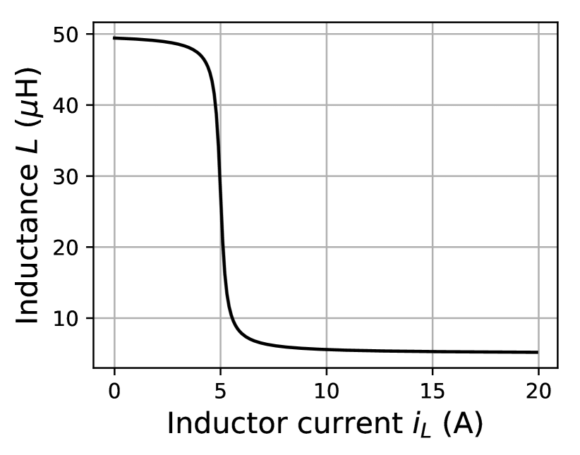
Figure 1: Nonlinear series RLC circuit used in the example (left) and nonlinear dependence of the inductance $L$ on the inductor current $i_{L}$ (right).

The circuit behavior is described by the continuous-time state-space equation

$$\begin{bmatrix}\dot{v}_{C}\\ \dot{i}_{L}\end{bmatrix}=\begin{bmatrix}0&\tfrac{1}{C}\\ \tfrac{-1}{L(i_{L})}&\tfrac{-R}{L(i_{L})}\\ \end{bmatrix}\begin{bmatrix}v_{C}\\ i_{L}\end{bmatrix}+\begin{bmatrix}0\\ \tfrac{1}{L(i_{L})}\end{bmatrix}v_{in},$$ (18)

where $v_{in}~{}\rm(V)$ is the input voltage; $v_{C}~{}\rm(V)$ is the capacitor voltage; and $i_{L}~{}\rm(A)$ is the inductor current. The circuit parameters $R=3~{}\Omega$ and $C=270$ nF are fixed, while the inductance $L$ depends on $i_{L}$ as shown in Fig. 1 (right). Specifically,

$$L(i_{L})=L_{0}\bigg{[}\bigg{(}\frac{0.9}{\pi}\arctan\big{(}-\!5(|i_{L}|-5\big{)}+0.5\bigg{)}+0.1\bigg{]},$$

with $L_{0}=50~{}{\mu\rm H}$. The identification dataset ${\mathcal{D}}$ is built by discretizing (18) using a $4$th-order Runge-Kutta method with a fixed step $T_{s}=0.5~{}\mu\text{s}$ and simulating the system for $2~{}\text{ms}$. $N=4000$ samples are gathered. The input $v_{in}$ is filtered white noise with bandwidth $150~{}\text{kHz}$ and standard deviation $80~{}\text{V}$. An independent validation dataset is generated using as input $v_{in}$ filtered white noise with bandwidth $200~{}\text{kHz}$ and standard deviation $60~{}\text{V}$.

The performance of the estimated models is assessed in terms of the $R^{2}$ index computed using the open-loop simulated model output. As reference, a second-order linear OE model estimated on noise-free data using the System Identification Toolbox [Ljung, 1988] achieves an $R^{2}$ index of $0.96$ for $v_{C}$ and $0.77$ for $i_{L}$ on the identification dataset, and $0.94$ for $v_{C}$ and $0.76$ for $i_{L}$ on the validation dataset.

We consider for neural model structures the cases of ($i$) noise-free measurements of $v_{C}$ and $i_{L}$; ($ii$) noisy measurements of $v_{C}$ and $i_{L}$; ($iii$) noisy measurements of $v_{C}$ only.

5.2 Algorithm setup

For gradient-based optimization, the Adam optimizer is used at Step 2.6 of Algorithm 1 to update the network parameters $\theta$ and the hidden variable $\overline{Y}$ (or $\overline{X}$ for state-space structures) used to construct the initial conditions $\mathbf{x}_{j,0}^{\mathrm{sim}}$. The learning rate $\lambda$ is adjusted through a rough trial and error, with $\lambda$ taking values in the range $[10^{-2}~{}10^{-6}]$, while the number of iterations $n$ is chosen large enough to reach a plateau in the cost function. In Algorithm 1, the weight $\alpha$ is always set to $0.5$. We tested different values for the sequence length $m$ and adjusted the batch size $q$ such that $qm\approx N$.

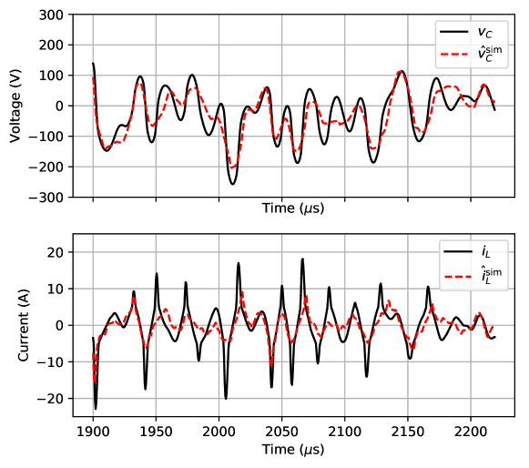
Figure 2: True output (black) and simulated output (red) obtained by the state-space model trained using the one-step prediction error minimization approach in the presence of noise.

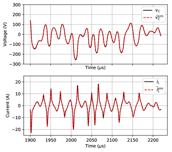
Figure 3: True output (black) and simulated output (red) obtained by the state-space model trained using the $64$-step simulation error minimization approach in the presence of noise.

5.3 Results

($i$) Noise-free measurements of $v_{C}$ and $i_{L}$  
Since in this case the system state is supposed to be measured, we use the fully-observed state model structure (5). The neural network $\mathcal{N\!N}_{x}$ modeling the state mapping has a sequential feedforward structure with three input units ($v_{C}$, $i_{L}$, and $v_{in}$); a hidden layer with 64 linear units followed by ReLU nonlinearity; and two linear output units—the two components of the state equation to be learned. Having a noise-free dataset, we expect good results from one-step prediction error minimization. Thus, we fit the model using this approach over $n=40000$ iterations with learning rate $\lambda=10^{-4}$. The time required to train the network is 114 seconds. The fitted model describes the system dynamics with high accuracy. On both the identification and the validation datasets, the model $R^{2}$ index in open-loop simulation is above $0.99$ for $v_{C}$ and $0.98$ for $i_{L}$.

($ii$) Noisy measurements of $v_{C}$ and $i_{L}$  
We consider the same identification problem above, with observations of $v_{C}$ and $i_{L}$ corrupted by an additive white Gaussian noise with standard deviation $10~{}\rm V$ and $1~{}\rm A$, respectively. This corresponds to a Signal-to-Noise Ratio (SNR) of 20 dB and 13 dB on $v_{C}$ and $i_{L}$, respectively. Results for the one-step prediction error minimization approach on the validation dataset are shown in Fig. 2. The $R^{2}$ index in validation drops to $0.73$ for $v_{C}$ and $0.03$ for $i_{L}$. It is evident that noise has a severe impact on the performance of the one-step method.

In the presence of noise, better performance is expected from a multi-step simulation error minimization approach. Thus, we fit the same neural state-space model structure using Algorithm 1 over $n=15000$ iterations, with $\lambda=10^{-3}$, and randomly extracted batches of $q=62$ subsequences, each of length $m=64$. The results are in line with expectations. Indeed, we recover similar performance as one-step prediction error minimization in the noise-free case ($R^{2}$ index of $0.99$ on $v_{C}$ and $0.98$ on $i_{L}$ on both the identification and the validation datasets). Time trajectories of the output are reported in Fig. 3. For the sake of visualization, only a portion of the validation dataset is shown. The total run time of Algorithm 1 is 182 seconds—about 60% more than the one-step prediction error minimization method.

Open-loop simulation error minimization is also tested. This method yields the same performance of $64$-step simulation error minimization in terms of $R^{2}$ index of the fitted model. However, it takes about two hours to execute $n=10000$ iterations required to reach a cost function plateau.

($iii$) Noisy measurements of $v_{C}$ only  
We consider the case where only the voltage $v_{C}$ is measured and corrupted by an additive white Gaussian noise with standard deviation $10$ V. The IO model structure in (7) is used with $n_{a}=2$ and $n_{b}=2$. The neural network $\mathcal{N\!N}_{\rm IO}$ is characterized by four input units (corresponding to $n_{a}=2$ previous values of $v_{C}$ and $n_{b}=2$ previous values of $v_{in}$); a hidden layer with 64 linear units followed by ReLU nonlinearity; and a linear output unit representing the output value $v_{C}$. As in case ($ii$), the one-step prediction error minimization approach delivers unsatisfactory results due to the presence of measurement noise. Thus, we fit the model using the multi-step method described in Algorithm 1 over $n=15000$ iterations, with $\lambda=10^{-3}$, $m=32$, and $q=124$. The total runtime of the algorithm is 192 seconds. The $R^{2}$ index of the fitted model is above $0.99$ on both the identification and the validation dataset, thus even larger than the $R^{2}$ index achieved by the OE model estimated on noise-free data.

6 Conclusions and follow-up

In this paper, we have presented neural model structures and fitting criteria for the identification of dynamical systems. A custom method minimizing a regularized multi-step simulation error criterion has been proposed and compared with one-step prediction error and simulation error minimization.

The main strengths of the presented framework are its versatility to describe complex non-linear systems, thanks to the neural network flexibility; its robustness to the measurement noise, thanks to the multi-step simulation error criterion with initial condition estimation; and the possibility to exploit parallel computing to train the network and optimize the initial conditions, thanks to the division of the dataset into small-size subsequences.

Current and future research activities are devoted to: ($i$) the formulation of proper fitting criteria and optimization algorithms for direct learning of continuous-time systems and systems described by partial differential equations, without introducing numerical discretization; ($ii$) the development of computationally efficient algorithms for estimation and control based on the neural dynamical models.

References

- Chen et al. [1990] S. Chen, S. Billings, and P. Grant. Non-linear system identification using neural networks. International journal of control, 51(6):1191–1214, 1990.
- Chen et al. [2018] T. Q. Chen, Y. Rubanova, J. Bettencourt, and D. K. Duvenaud. Neural ordinary differential equations. In Advances in neural information processing systems, pages 6571–6583, 2018.
- Gonzalez and Yu [2018] J. Gonzalez and W. Yu. Non-linear system modeling using lstm neural networks. IFAC-PapersOnLine, 51(13):485–489, 2018.
- Hornik et al. [1989] K. Hornik, M. Stinchcombe, and H. White. Multilayer feedforward networks are universal approximators. Neural networks, 2(5):359–366, 1989.
- Kingma and Ba [2014] D. P. Kingma and J. Ba. Adam: A method for stochastic optimization. arXiv preprint arXiv:1412.6980, 2014.
- Ljung [1988] L. Ljung. System identification toolbox. The Matlab user’s guide, 1988.
- Ljung [1999] L. Ljung, editor. System Identification: Theory for the User. Prentice Hall PTR, Upper Saddle River, NJ, USA, 2 edition, 1999. ISBN 0-13-656695-2.
- Masti and Bemporad [2018] D. Masti and A. Bemporad. Learning nonlinear state-space models using deep autoencoders. In 2018 IEEE Conference on Decision and Control (CDC), pages 3862–3867, 2018.
- Paszke et al. [2017] A. Paszke, S. Gross, S. Chintala, G. Chanan, E. Yang, Z. DeVito, Z. Lin, A. Desmaison, L. Antiga, and A. Lerer. Automatic differentiation in PyTorch. In NIPS Autodiff Workshop, 2017.
- Raissi et al. [2019] M. Raissi, P. Perdikaris, and G. E. Karniadakis. Physics-informed neural networks: A deep learning framework for solving forward and inverse problems involving nonlinear partial differential equations. Journal of Computational Physics, 378:686–707, 2019.
- Rumelhart et al. [1988] D. E. Rumelhart, G. E. Hinton, R. J. Williams, et al. Learning representations by back-propagating errors. Cognitive modeling, 5(3):1, 1988.
- Schmidhuber [2015] J. Schmidhuber. Deep learning in neural networks: An overview. Neural networks, 61:85–117, 2015.
- Wang [2017] Y. Wang. A new concept using lstm neural networks for dynamic system identification. In 2017 American Control Conference (ACC), pages 5324–5329, 2017.
- Werbos [1989] P. J. Werbos. Neural networks for control and system identification. In Proceedings of the 28th IEEE Conference on Decision and Control,, pages 260–265, 1989.
- Williams and Zipser [1995] R. J. Williams and D. Zipser. Oxford Handbook of Innovation, chapter Gradient-Based Learning Algorithms for Recurrent Networks and Their Computational Complexity. L. Erlbaum Associates Inc., Hillsdale, NJ, USA, 1995.