Mean-field approximation for structural balance dynamics in heat-bath

Abstract

A critical temperature for a complete signed graph of $N$ agents where time-dependent links polarization tends towards the Heider (structural) balance is found analytically using the heat-bath approach and the mean-field approximation as $T^{c}=(N-2)/a^{c}$, where $a^{c}\approx 1.71649$. The result is in perfect agreement with numerical simulations starting from the paradise state where all links are positively polarized as well as with the estimation of this temperature received earlier with much more sophisticated methods. When heating the system, one observes a discontinuous and irreversible phase transition at $T^{c}$ from a nearly balanced state when the mean link polarization is about $x_{c}=0.796388$ to a disordered and unbalanced state where the polarization vanishes. When the initial conditions for links polarization are random, then at low temperatures a balanced bipolar state of two mutually hostile cliques exists that decays towards the disorder and there is a discontinuous phase transition at a temperature $T^{d}$ that is lower than $T^{c}$. The system phase diagram corresponds to the so-called fold catastrophe when a stable solution of the mean-field equation collides with a separatrix, and as a result a hysteresis-like loop is observed.

I Introduction

Let $i$ and $j$ be persons and $k$ be an object that could be a third person, article, idea, event, etc. If the persons $i$ and $j$ possess the same attitude towards the object $k$ (e.g. they both like or both dislike it) then the theory of structural balance postulated by Heider Heider (1946) says that it is more probable there is a positive relation between $i$ and $j$. On the other hand, if there is a disagreement between the attitudes of $i$ and $j$ towards $k$, then it is more likely that there is a negative relation between $i$ and $j$. In the case where $k$ is a person, the above propositions can be formed as the following rules: friend of my friend is my friend, enemy of my enemy is my friend, friend of my enemy is my enemy and enemy of friend is my enemy.

Structural balance theory met a lot of interest in social science and it was observed in many social groups when friendships and antipathies could be detected, see, e.g., References Harary, 1953; Cartwright and Harary, 1956; Harary, 1959; Davis, 1967; Harary et al., 1965; Doreian and Mrvar, 1996; Rambaran et al., 2015; Rawlings and Friedkin, 2017; Chiang and Tao, 2019; Toroslu and Jaspers, 2022; Bramson et al., 2022. Antal, Krapivsky and Redner Antal et al. (2005, 2006) found a way to use the master equation for a description of possible dynamics of complex networks evolving toward the structural balance when mutual attitudes are described by binary variables of corresponding links.

Nowadays there are several attempts at theoretical description and computational simulation of the Heider balance, for example, when the attitudes are continuously changing variables Kułakowski et al. (2005); Marvel et al. (2011); Gawroński et al. (2015) or when attitudes are link attributes following from Hamming distances between nodes attributes Górski et al. (2020a). Often, an interpersonal relationship between two agents evolves, driven by the products of their relations (positive or negative) with their common neighbors. In this way, two friendly or two hostile relations of two agents with their common neighbor improve their mutual relation, while their different relations with a neighbor drive their mutual relation to hostility. For example, in References Kułakowski et al., 2005; Marvel et al., 2011, the relations are represented by real numbers, and the system dynamics—by a set of differential equations. In these papers, the network of relations is a complete graph. In References Malarz et al., 2020; Malarz and Kułakowski, 2021a the relations are either positive or negative, and the dynamics is defined by a cellular automaton deterministic or with a thermal noise, and a local neighborhood of different range. In References Krawczyk et al., 2021; Burda et al., 2022 the relations are also discrete, the automaton rule is deterministic and the topology is a complete graph. In all these approaches, the target is a balanced state, i.e., a partition of the graph into two mutually hostile but internally friendly groups. When the sign of the relation of a pair as in Reference Burda et al., 2022 is assumed to oscillate with the sum of products of relations over their neighbors, this target is reached immediately—in one time step—for each initial state Krawczyk and Kułakowski (2022). For other approaches see References Estrada and Benzi, 2014; *Nishi_2014; *Kovchegov_2016; *Gorski_2017; *Krawczyk_2019; *PhysRevLett.125.078302; *Sheykhali_2020; *Pham_2021; *Deng_2021; *Arabzadeh_2021; *PhysRevE.105.054105; *Krawczyk_2015; *Stojkow_2020; *Krawczyk_2021.

Recently Rabbani et al. (2019); Shojaei et al. (2019); Malarz and Kułakowski (2021b); Manshour and Montakhab (2021); Malarz and Wołoszyn (2020); Wołoszyn and Malarz (2022); Malarz and Wołoszyn (2022), the Heider’s dynamics has been enriched with social temperature $T$ Kułakowski (2008). In Reference Rabbani et al., 2019 authors show that in the investigated system the first-order phase transition from ordered to disordered state is observed. A system of two coupled algebraic equations has been received using a mean-field approximation for an average link polarization and a correlation function between neighboring links polarization. The critical temperature of the complete graph consisting of $50$ nodes has been estimated by numerical solutions of these equations and agent based simulations confirmed the presence of the phase transition transition in such a model. In this paper, we show a much simpler theoretical approach leading to the same conclusions. Similarly as in Reference Rabbani et al., 2019 we use the mean-field approximation but we find the critical temperature $T_{c}$ only from the average value of link polarization and we show that $T_{c}$ is proportional to number $M$ of different triangles containing a given link $T^{c}=M/1.71649\cdots$. If a network with all positive links is heated then the discontinuous phase transition takes place when the mean link polarization decays to the critical value $x_{c}=0.796388$. Our analytical results are well supported with computer simulation.

Figure 1: Heider’s triads corresponding to balanced (first and third) and imbalanced (second and fourth) states

II Model

Consider a network of $N$ agents, and let us assume that the polarization of the links between two agents $i$ and $j$ is $x_{ij}=\pm 1$. The dynamics towards the Heider balance can be written as

$$x_{ij}(t+1)=\operatorname{\mathrm{sign}}\left(\sum_{k}^{M_{ij}}x_{ik}(t)x_{kj}(t)\right),$$ (1)

where the summation goes through $M_{ij}$ common nearest neighbors of the connected nodes $i$ and $j$, that is, $M_{ij}$ is the number of triangles that involve the link ${ij}$. It means that for a single triangle system presented in Figure 1 the first and third triangles are balanced in the Heider’s sense (as friend of my friend is my friend and enemy of my friend is my enemy), while the second and the fourth are not. In the latter case actors at triangles nodes either encounter the cognitive dissonance—as they cannot imagine how his/her friends can be enemies—or everybody hates everybody, which should lead to creation of a two-against-one coalition. Let us stress that formally the sum $\sum_{k}^{M_{ij}}x_{ik}(t)x_{kj}(t)$ can be treated as a local field acting on the link $x_{ij}$ and this field follows from the Hamiltonian Antal et al. (2005); Rabbani et al. (2019)

$$\mathcal{H}=-\sum_{i>j>k}^{N}x_{ij}x_{jk}x_{ki}.$$ (2)

III Mean-field analytical approach

If one assumes that the link dynamics possesses a probabilistic character, then a natural form of updating rule (1) as in Heider dynamics can be:

$$x_{ij}(t+1)=\begin{cases}+1&\text{ with probability }p_{ij}(t),\\ -1&\text{ with probability }1-p_{ij}(t),\end{cases}$$ (3a)

where

$$p_{ij}(t)=\frac{\exp(\xi_{ij}(t)/T)}{\exp(\xi_{ij}(t)/T)+\exp(-\xi_{ij}(t)/T)}$$ (3b)

and

$$\xi_{ij}(t)=\sum_{k}^{M_{ij}}x_{ik}(t)x_{kj}(t).$$ (3c)

Here, the positive variable $T$ can be considered as a social temperature Kułakowski (2008) (or a measure of the noise amplitude) and in the limit $T\to 0^{+}$ we have $p\to 1$ so Equation 3 reduces to Equation 1. Equation 3 is nothing else but the heat-bath algorithm (Binder, 1997, p. 505) for a stochastic version of Equation 1 and thus it is ready for direct implementation in analytical investigations and computer simulations.

The expected value $\langle x_{ij}(t+1)\rangle$ in this approach is equal to

$$\langle x_{ij}(t+1)\rangle=\tanh\left(T^{-1}\sum_{k}^{M_{ij}}x_{ik}(t)x_{kj}(t)\right),$$ (4)

where $\langle\cdots\rangle$ stands for a mean value related to the stochastic process defined by Equation 3.

The mean $\langle x_{ij}(t+1)\rangle$ is a continuous variable that can be negative or positive, and for $T\to 0^{+}$ the Equation 4 reduces to Equation 1.

Now in our mean-field approximation we write the correlation function $\langle x_{ik}(t)x_{kj}(t)\rangle$ as the product $\langle x_{ik}(t)\rangle\langle x_{kj}(t)\rangle$. Let us note that such an approximation for the correlation function of link polarization is similar to the mean-field assumption used for the Ising model where correlations between spins $S_{i}$, $S_{j}$ are neglected, i.e. $\langle S_{i}S_{j}\rangle=\langle S_{i}\rangle\langle S_{j}\rangle$ see e.g. Reference Wu, 1966. In fact, in Reference Rabbani et al., 2019 another mean-field approach was proposed where link-link correlations were considered but as we demonstrate in the Appendix A they can be disregarded in the thermodynamical limit of the studied system. Then instead of Equation 4 we have

$$\{\langle x_{ij}(t+1)\rangle\}\approx\tanh\left(\frac{1}{T}\sum_{k}^{M_{ij}}\{\langle x_{ik}(t)\rangle\}\{\langle x_{kj}(t)\rangle\}\right),$$ (5)

where $\{\cdots\}$ denotes the average over all $N(N-1)/2$ available nodes’ pairs.

Now let us assume—also in agreement with the spirit of mean-field approximation—that all averages are the same

$$\{\langle x_{ij}\rangle\}=\{\langle x_{ik}\rangle\}=\{\langle x_{kj}\rangle\}=x.$$ (6)

The above approximations are justified in the neighborhood of paradise state where the majority of triangles of type 1(a) are present. However, as we show in further numerical simulations, the approach also works well in states far from paradise ($x\approx 0$).

It follows that we get

$$x(t+1)=\tanh[ax^{2}(t)],$$ (7)

where

$$a=M/T,$$ (8)

and $M=\{M_{ij}\}$ is the average number of common neighbors of agents $i$ and $j$ (it also the number of different triads containing the edge $ij$).

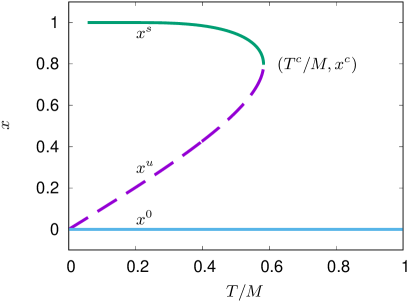
Figure 2: Solutions for mean values of links polarizations in Heider balance resulting from the mean field approximation $x=\tanh(ax^{2})$. At the point $T^{c}/M=1/a^{c}\approx 0.582584\cdots$ ($x^{c}\approx 0.796388\cdots$) a discontinuous transition between the upper branch and the solution $x=0$ takes place.

We immediately recognize $x^{0}=0$ as a stable fixed point for any value of the $a$ parameter, and for $a\ll 1$ this is the only fixed point of Equation 7. However, for $a\gg 1$ there are two other fixed points, $x^{u}<x^{s}$ corresponding to unstable $x^{u}(a)$ and stable $x^{s}(a)$ solutions. In fact, $x^{u}$ is a separatrix between the domain of attractions of fixed points $x^{0}$ and $x^{s}$. When $a\gg 1$ then $x^{u}\approx 1/a$. When the parameter $a$ decreases from high values (this means that the temperature $T$ increases), then the fixed points $x^{u}$ and $x^{s}$ coincide together with the point $x^{c}$ for a certain value of $a=a^{c}$ (see Figure 2).

This means that for $a>a_{c}$ the system is bi-stable and for $a<a^{c}$ the system is mono-stable. The above values $a^{c},x^{c}$ can be received from a pair of transcendental algebraic relations that describe the fixed point and its tangency condition, namely

$$x^{c}=\tanh\left(a^{c}(x^{c})^{2}\right)$$ (9a)

and

$$2a^{c}x^{c}=\cosh^{2}\left(a^{c}(x^{c})^{2}\right).$$ (9b)

The solutions (see Figure 2) are

$$x^{c}_{\text{th}}\approx 0.796388\cdots$$ (10a)

and

$$a^{c}_{\text{th}}=\tanh^{-1}(x^{c}_{\text{th}})/(x^{c}_{\text{th}})^{2}\approx 1.71649\cdots.$$ (10b)

Let us note that since $x^{c}_{\text{th}}>0$ a system can express the phenomenon of hysteresis. It also means that we should not observe the values $0<x<x^{c}_{\text{th}}$ as stable solutions.

IV Numerical estimation of system critical temperature

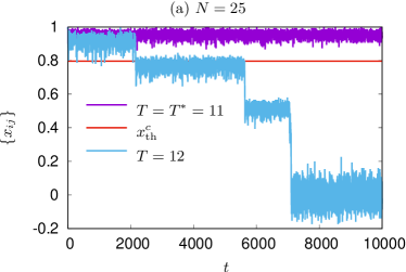
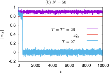
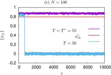
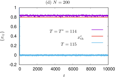
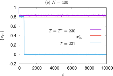
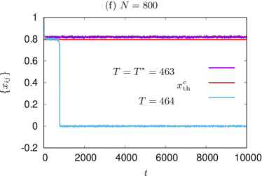
Figure 3: The time evolution of the average values of all links polarization $\{x_{ij}\}$ for various social temperature $T$ and various system sizes $N$. The starting point of simulation is homogeneous state (paradise) with $\{x_{ij}\}=+1$ and the scanning temperature step is $\Delta T=1$. When the temperature $T=T^{*}$ then averages $\{x_{ij}\}$ oscillate around values that are close but always larger than the critical solution $x^{c}$ (the solid red line given by the mean field approach (10a)) however when the temperature $T$ is slightly above $T^{*}$ the system evolves towards the state $\{x_{ij}\}\approx x^{0}=0$.

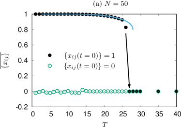
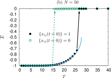
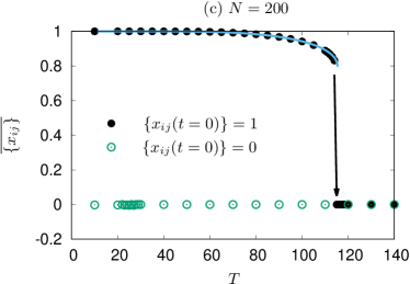
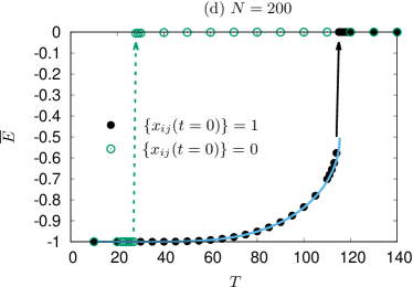
Figure 4: (Color online). Panels (a, c) show the averages $\overline{\{x_{ij}\}}$ and the panels (b, d) $\overline{E}$ as functions of the temperature $T$ for complete graph with $N=50$ (a, b) and $N=200$ (c, d) nodes. The averaging symbol $\overline{\cdots}$ stands for time average over the last $\tau=1000$ time steps of simulation. The solid symbols correspond to the paradise state as the starting point. The open symbols stand for random initial state $\{x_{ij}\}=0$. The solid blue lines indicate the mean-field approximation predictions $\overline{\{x_{ij}\}}=x$ (a, c) and $\overline{E}=-x^{3}$ (b, d). The solid black or dashed green arrow marks the positions of the critical temperature $T^{c}$ or $T^{d}$ (see Section V).

Table 1: The numerically obtained values of $T^{c}_{\text{nu}}$ and $a^{c}_{\text{nu}}$ calculated basing on Equation 11a together with their estimated expanded uncertainties $U(a^{c}_{\text{nu}})$. The uncertainty of $T^{c}_{\text{nu}}$ is $u(T^{c}_{\text{nu}})=1/\sqrt{3}$, while $U(a^{c}_{\text{nu}})$ is calculated basing on Equation 11b. Note that the differences between numerically estimated values and analytical results (values in the last column) are smaller than the uncertainties $U(a_{\text{nu}}^{c})$.

$N$	$T^{c}_{\text{nu}}$	$a^{c}_{\text{nu}}$	$U$$(a^{c}_{\text{nu}})$	$a^{c}_{\text{nu}}-a^{c}_{\text{th}}$
25	11.5	2.00	0.30	0.28
50	26.5	1.811	0.118	0.095
100	55.5	1.766	0.055	0.049
200	114.5	1.7293	0.0262	0.0128
400	320.5	1.7267	0.0130	0.0102
800	463.5	1.7217	0.0064	0.0052

To verify the analytical results in computer simulation, we directly apply Equation 3 to the time evolution of $x_{ij}$ for the complete graph with $N$ nodes. For the complete graph the average number of pair neighbors of nodes $ij$ is equal to $M=\{M_{ij}\}=N-2$ and thus according to Equation 8 one should expect

$$a^{c}_{\text{nu}}=(N-2)/T^{c}_{\text{nu}}.$$ (11a)

To find the value of $T^{c}_{\text{nu}}$ we start the simulation with $T=0$ and scan the temperature $T$ with step $\Delta T$ and look for a value of $T^{*}$ for which $\langle x_{ij}\rangle$ is positive but for $T^{*}+\Delta T$ is zero. The true value of $T^{c}_{\text{nu}}$ is hidden somewhere in the interval $[T^{*},T^{*}+\Delta T]$. We assume that $T^{c}$ value is uniformly distributed in the interval $[T^{*},T^{*}+\Delta T]$ which allows us to estimate its uncertainty as $u(T^{c}_{\text{nu}})=\Delta T/\sqrt{3}$. The estimated value of $T^{c}_{\text{nu}}=(T^{*}+T^{*}+\Delta T)/2$. Based on Equation 8 we calculate the value of $a^{c}_{\text{nu}}$ and we can estimate its expanded uncertainty as

$$U(a^{c}_{\text{nu}})={k}\left|\dfrac{\partial a}{\partial T}\right|_{T=T^{c}}u(T^{c}_{\text{nu}})={k}\dfrac{N-2}{(T^{c}_{\text{nu}})^{2}}u(T^{c}_{\text{nu}}),$$ (11b)

with the coverage factor $k=3$ Taylor and Kuyatt (1994).

In Figure 3 the time evolution of $\{x_{ij}\}$ for various values of social temperature $T$ and various system sizes $N$ is presented. The starting point of the simulation is the homogeneous state (paradise) with $\{x_{ij}\}=+1$ and the scanning temperature step is set to $\Delta T=1$. The solid red line corresponds to $x^{c}_{\text{th}}$ given by Equation 10a.

The obtained critical temperatures $T^{c}_{\text{nu}}$ and their uncertainties $U(T^{c}_{\text{nu}})$ are collected in Table 1. The obtained values of $a^{c}_{\text{nu}}$ coincide nicely with those obtained analytically (see Equation 10b) even under very crude assumptions given by Equation 7. The values of $a^{c}_{\text{nu}}$ agree within expanded uncertainties $U$$(a^{c}_{\text{nu}})$ with its analytical partner $a^{c}_{th}$.

In Figure 4(a), (c) the dependencies of $\overline{\{x_{ij}\}}$ vs. $T$ for $N=200$ and $N=50$ are presented. The averaging symbol $\overline{\cdots}$ represents the time average in the last $\tau=100$ time steps of the simulation, and this time average should be approximately equal to the average $\langle\cdots\rangle$ used in Equation 5, which comes from the ergodic theorem. Solid symbols correspond to the starting point $\forall i,j:x_{ij}=+1$, while open symbols represent a random initial state $\{x_{ij}\}=0$. The latter recovers $x^{0}=0$ mentioned earlier.

In Figure 4(b), (d) dependencies of the system energy density (average value of the Hamiltonian (2) per triangle)

$$E=-\dfrac{\sum_{i>j>k}x_{ij}x_{jk}x_{ki}}{\binom{N}{3}}$$ (12)

are presented. There is a discontinuous change in the mean system energy at the critical temperature, this corresponds to Figure 4(b) in Reference Rabbani et al., 2019. According to the mean-field approximation Equation 6 we expect $E=-x^{3}$, and this approximation is marked by a solid blue line in Figure 4(b), (d). Similarly to the numerically obtained values of $\overline{\{x_{ij}\}}$ also values of $\overline{E}$ agree fairly with the proposed mean-field approximation.

V Influence of mutually hostile cliques on critical behavior

In previous Sections we estimated analytically and numerically the value of the system critical temperature $T_{c}$ when initial conditions were close to the paradise state. We observed however that when a random initial state $\{x_{ij}(t=0)\}=0$ was used in our numerical simulations then a transition to a phase with a higher energy $\overline{E}=0$ took place at a temperature $T^{d}$ that was lower than $T^{c}$. Below we discuss the nature of this transition (see also Reference Malarz and Kułakowski, 2021b).

For random initial conditions the observed average $\{x_{ij}\}$ fluctuates around zero in time but the mean energy density is $\overline{E}=-1$ (see Figure 4) in low temperatures. In other words, this energy is the same as the system energy corresponding to the paradise state (with only positive links) $\{x_{ij}\}=1$. This means that the ground state of the system is degenerated Krawczyk et al. (2017). Although the fact that the state $\{x_{ij}\}=0$ is stable in time follows from Equation 7 its nature can be seen to be strange, since naively one would expect a picture of a disordered system corresponding to many unbalanced triangles with $\overline{E}=0$ and not $\overline{E}=-1$.

Figure 5: An example of bipolar state with two mutually hostile cliques of sizes $h=4$. Each node possesses $(h-1)$ positive links to agents in the own clique and $h$ negative links to the second clique.

The truth is that the stochastic evolution Equation 3 starting from the unordered state $\{x_{ij}\}=0$ can lead to a polarized phase consisting of two paradises (cliques containing only friendship triangles 1(a)) of similar sizes (for entropic reasons) connected by hostile triangles 1(c)—see Figure 5. Such a balanced state composition has already been predicted for systems driven by the structural balance by Cartwright and Harary (1956) in the middle ‘50. The phase was observed also in the model of constrained triad dynamics (CTD) introduced by Antal Antal et al. (2005, 2006) when a randomly selected link flips its temporal polarization $x_{ij}$ only if the total number of imbalanced triad decreases (see also Reference Malarz et al., 2020). Such a case corresponds to Equation 1 and it is equivalent to $T\to 0^{+}$ limit of heat-bath Equations (3).

Let us assume that the size of the entire group is an even number $N=2h$ and that each hostile group has the size $h$. Such a partition is the most probable division of the entire group Antal et al. (2005, 2006) and it is then easy to show that the mean of $\{x_{ij}\}$ is zero in such a bipolar phase. In fact, every node possesses $(h-1)$ positive links to agents in the own group and $h$ negative links to the second group. It follows that the mean link polarization $\{x_{ij}\}$ is equal to $-1/(2h-1)$ and vanishes in the thermodynamic limit ($h\to\infty$). Then, the number of triangles 1(a)

$$n_{\Delta}(+3)=2\binom{h}{3}=\frac{1}{3}h(h-1)(h-2)$$ (13)

and the number of triangles 1(c)

$$n_{\Delta}(-1)=2h\binom{h}{2}=h^{2}(h-1)$$ (14)

may be calculated with combinatorial analysis due to the complete graph symmetry. It follows that in the thermodynamic limit, there is a special ratio between the numbers of triangles 1(c) and number of triangles 1(a) in this phase

$$\lim_{h\to\infty}\frac{n_{\Delta}(-1)}{n_{\Delta}(+3)}=3$$ (15)

and due to the absence of unbalanced triangles 1(b) and 1(d) in this phase the frequencies of triads presented in Figure 1 are $(\frac{1}{4},0,\frac{3}{4},0)$.

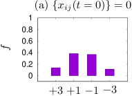
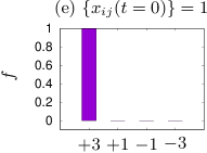
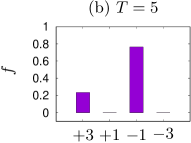
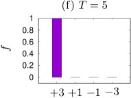
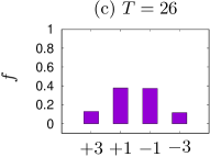
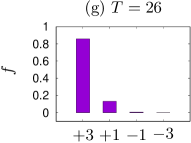
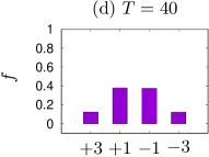
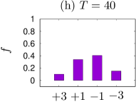
Figure 6: Frequencies $f$ of appearing of triangles presented in Figure 1 for $N=50$ and various initial states. In the first row the histograms for initial states are presented. In left (right) column histograms for random (paradise) initial states are presented. In rows 2–4 the histograms of frequencies of various triangles types in the final state of the systems are presented. The assumed temperatures $T$ are indicated in subfigures headlines. The numbers on abscissa axis are sum of polarizations $x_{ij}$ in a given triangle presented in Figure 1.

To verify our picture, we numerically investigated the frequencies $f$ of different triangles in the network when we start the evolution of the system from various initial conditions. These frequencies are presented in Figure 6. When we start from $\{x_{ij}\}=0$ then for low temperatures (see Figure 6(b)) the observed fraction $f(+3)$ of triangles 1(a) is three times lower than the fraction $f(-1)$ of triangles 1(c) as predicted by Equation 15. The fractions of triangles presented in Figure 1 change abruptly from $(\frac{1}{4},0,\frac{3}{4},0)$ to $(\frac{1}{8},\frac{3}{8},\frac{3}{8},\frac{1}{8})$ at a critical temperature $T_{d}$ (see Figure 6(c)–(d), cf. also Figure 10 in Reference Wołoszyn and Malarz, 2022). The latter distribution of various types of triads is also kept in high temperature when we start the temporal system evolution from the paradise state (see Figure 6(h)) and it corresponds to the probabilities of three, two, one, and zero successes in three Bernoulli trials when the probability of success is equal to $\frac{1}{2}$.

The above results mean that the polarized state with two hostile cliques exists only at low temperatures and disappears abruptly at $T=T^{d}$. Let us stress that cliques emerge from random initial conditions in our numerical simulations. A similar discontinuous transition was observed in CTD dynamics in References Antal et al., 2005, 2006 when the initial density of positive links and the average $\{x_{ij}(t=0)\}$ were changed in a continuous way. The analytical approach developed in Reference Antal et al., 2006 shows that the critical value of $\{x_{ij}(t=0)\}$ for this transition should be equal to zero. When this average is smaller, then the system reaches an equilibrium in the two cliques state, and above this threshold the system evolves towards the paradise. Numerical simulations for the CTD model show a slightly higher value of this threshold Antal et al. (2006). This discontinuous transition can be understood using our mean-field approach developed in Section III as a result of the multistability of the system presented in Figure 2. In fact, the unstable solution $x^{u}$ of Equation 7 in Figure 2 divides the set of initial conditions into two basins of attraction Ott (2002); *Kacperski_1996. When $\{x_{ij}(t=0)\}$ is below $x^{u}$ the system evolves towards the solution $x^{0}=0$ and for an initial condition above this curve the system evolves towards $x^{s}$. Since our model at $T=0$ corresponds to the CTD model and the separatrix $x^{u}$ in Figure 2 approaches zero at this limit, the discontinuous disappearance of the polarized two-cliques phase observed in Reference Antal et al., 2006 can be explained by crossing the separatrix curve. This critical behavior is equivalent to the bifurcation diagram corresponding to the so-called fold catastrophe Scheffer et al. (2009) and similar discontinuous phase transitions resulting from system bistability were observed in many systems, including pairs of weakly interacting Ising networks Suchecki and Hołyst (2009); *PhysRevE.74.011122, a majority model of a network with communities Lambiotte et al. (2007), as well as an activity-driven temporal bilayer echo-chamber system Gajewski et al. (2022).

VI Conclusions

In this paper we present a simple analytical approach, which describes the first-order phase transition observed in thermalized Heider’s balance systems on the complete graphs. The proposed mean-field approximation predicts that the critical temperature of the system is equal to $T^{c}=(N-2)/a^{c}$, where $N$ is the number of graph nodes, and $a^{c}\approx 1.71649$. This temperature corresponds to a discontinuous transition from a critical state $\{x_{ij}\}=x^{c}\approx 0.796388$ (that is close to the paradise state) to an unbalanced state with the same number of positive and negative links $\{x_{ij}\}=x^{0}=0$. At the critical point $(T_{c},x_{c})$ the upper stable solution $x^{s}(T)$ for a fixed point of Equation (8)—corresponding to a state of paradise dressed with thermal fluctuations at a given temperature $T$—coincides with the unstable branch $x^{u}(T)$ that is a separatrix, i.e. a boundary between initial conditions leading to the “nearly paradise” solution $x^{s}(T)$ or to the disordered solution $x^{0}$. For $T>T_{c}$ the solution $x^{s}(T)$ does not exist anymore and the system is always evolving towards $x^{0}$. This bifurcation scenario corresponds to the well-known fold catastrophe [see Figures 4(a) and 4(c)].

At the critical point, the system energy density changes from $\overline{E}=-(x^{c})^{3}$ to the value $\overline{E}=0$ [see Figures 4(b) and 4(d)]. The results of computer simulations agree within the estimated uncertainties with our analytical calculations providing that initial conditions are close to the paradise state $\{x_{ij}(t=0)\}=1$.

On the other hand, at any temperature $T$ when starting from a randomly selected state $x_{ij}=\pm 1$—when $\{x_{ij}(t=0)\}=0$—we reach in the simulation only the solution $\{x_{ij}\}=0$ corresponding to the stable fixed point $x^{0}$. The solution can correspond to various patters of polarizations $x_{ij}$. At low temperatures, there is a phase consisting of two cliques of similar sizes that possess only positive internal links, but all inter-cliques links are negative. It follows that there are triangles consisting of all positive links or triads of one positive link and two negatives. It means that all the triads are balanced and that the energy density of the system is the same as in the paradise state, $\overline{E}=-1$, that is, degeneration of the ground is observed. The signatures of such system division—i.e., the ratio $f(-1)\div f(+3)=75\%\div 25\%$—for low temperature noise level limit were also observed for diluted and densified triangulations (see Fig. 10 in Reference Wołoszyn and Malarz, 2022) and classical (Erdős–Rényi) random graphs (see Fig. 7 in Reference Malarz and Wołoszyn, 2022).

At a certain temperature $T=T^{d}$ [for $\{x_{ij}(t=0)\}=0$] or $T=T^{c}>T^{d}$ [for $\{x_{ij}(t=0)\}=1$] another discontinuous phase transition occurs when the number of unbalanced triads [1(b) and 1(d)] abruptly increases, and as a result the system energy density becomes zero [see dashed arrows connecting open symbols in Figures 4(b) and 4(d)]. This transition is not seen at a value of $\{x_{ij}\}$, which is zero below and zero above $T^{d}$ when $\{x_{ij}(t=0)\}=0$.

We stress that for $T^{d}<T<T^{c}$—depending on the initial conditions—the system energy is either close to the ground state or equal to zero [see Figures 4(b) and 4(d)]. Assuming initial conditions $\{x_{ij}(t=0)\}=1$ and heating the system from $T=0$ to $T=T^{c}$ decreases the mean value of $\{x_{ij}\}$ along the curve $x^{u}(T)$ to the critical point $x^{c}$, but above $T^{c}$ we can only reach $\{x_{ij}\}=0$. The observed transition is irreversible, and cooling the system from $T>T^{c}$ towards $T\to 0^{+}$ will never reproduce positive values of $\{x_{ij}\}>0$ and in this sense the hysteresis-like loop can be observed in the system, thus $(T_{c},x_{c})$ is a tipping point of our phase diagram Scheffer et al. (2009).

The critical temperature $T^{c}=26.2$ for the complete graph with $N=50$ nodes estimated in Reference Rabbani et al., 2019 is roughly in agreement with our estimate of $T^{c}$ for $N=50$. Finding analytically the value of a lower critical temperature $T^{d}$—where, starting with $\{x_{ij}(t=0)\}=0$, a special mixture of only balanced triangles 1(a) and 1(c) disappears—is beyond predictions of our approach, and it remains a challenge.

The most interesting result of these investigations for real social networks could be the observation that if such networks are driven by structural balance dynamics, then the balanced bipolar state seems to be the only possible state when the initial configuration of social links is completely random and the strengths of social interactions increase over time. To prohibit the emergence of such a polarized state, one could consider introducing additional attributes of interacting agents Górski et al. (2022).

Finally, we note that Heider’s theory may be applied for studies of international relations. In Reference Antal et al., 2005 authors presented the evolution of relations between countries as a prelude to World War I. Further analysis of historical data is in progress Estrada et al. (2022).

Appendix A

In the mean-field approximation developed in Reference Rabbani et al., 2019 the mean polarization of links is given as

$$p=\langle x_{ij}\rangle=\tanh(\beta(N-2)q),$$ (16)

where $\beta=1/T$ and $q=\langle x_{ik}x_{kj}\rangle$ is a correlation between links and

$$q=\frac{e^{2(N-3)\beta q}-2e^{-2\beta p}+e^{-2(N-3)\beta q}}{e^{2(N-3)\beta q}+2e^{-2\beta p}+e^{-2(N-3)\beta q}}.$$ (17)

Then the values $p$ and $q$ were found numerically as functions of the temperature $T$ from Equations (16) and (17) in Reference Rabbani et al., 2019. In our case, we receive the mean-field solution from the fix point of Equation (7), that is, $\langle x_{ij}\rangle=\tanh(\beta(N-2)\langle x_{ij}\rangle^{2})$. However, one can easily find that when $N\gg 1$ then

$$p^{2}\approx q.$$ (18)

In fact, in the thermodynamic limit, the difference between $q$ and $p^{2}$ is due to the second term of the nominator of Equation (17) which is $z=2\exp(-2\beta p)$ that should be equal to $2$ if Equation (18) is valid. However, one can write $z=2\exp(-(2p/T_{c})(T_{c}/T))$ where $T_{c}$ is a critical temperature and since every link is influenced by many triangles in the Hamiltonian (2) thus $T_{c}\gg 1$. Thus, when the system is in the critical region and $T\approx T_{c}$ then since $p/T_{c}\ll 1$ thus $z\approx 2$ and $p\approx q^{2}$. The approximation also works well in the low temperature region $T\to 0^{+}$ since in such a case the terms $z$ and $2$ are much smaller than the first term in the nominator of Equation (17) and $q=1$.