Classical Statistical simulation of Quantum Field Theory
Takayuki Hirayama
hirayama@isc.chubu.ac.jpDepartment of Mathematical and Physical Sciences,
College of Science and Engineering, Chubu University
1200 Matsumoto, Kasugai, Aichi, 487-8501, Japan
Abstract
We propose a procedure of computing the n-point function in perturbation theory of the quantum field theory as the average over the complex Gaussian noises in a classical theory.
The complex Gaussian noises are the sources
for the creation and annihilation of particles and the energy of the
resultant configuration is the same as the zero point energy of the corresponding quantum field theory.
I Introduction
In quantum field theory, the vacuum state is the lowest energy state and
its energy is the sum of , the zero point energy in the
free theory. The particles are continuously created and annihilated from
the vacuum. These properties lead us to the idea that we mimic the
quantum vacuum by the configuration in a classical theory with Gaussian random noises at each spacetime point which are the sources for the
creation and annihilation of particles. Then it is easily computed that
with the Gaussian noises, the configuration becomes non trivial and
its energy is equal to
the zero point energy in the quantum field theory. We will perturbatively
show that the average of n-point function over the noises is exactly
equal to the value of n-point function in quantum field theory.
It has been known that in the non trivial background some of the quantum behaviors are realized in a classical theory. In Boyer:1975re ; Boyer:1975rf , the each momentum modes of the electromagnetic fields have the
amplitude with and random phases. Then the motion of a
charged particle in the non trivial electromagnetic fields shows some of quantum phenomena such as the blackbody radiation, the decrease of
specific heats at low temperatures, and the absence of atomic collapse. In Hirayama:2005ba ; Hirayama:2005ac ; Holdom:2006tt , the random phase for each mode in the scalar field is introduced and then the zero point energy of the scalar field is realized in the classical theory. Then the loop Feynman graphs appear in the n-point function of scalar field, although not all the loop Feynman graphs in the quantum field theory appear.
It has been also known that when the occupation number is large, the
classical statistical approximation or the classical statistical Lattice
simulation, is a good approximation to the quantum field theory Aarts:1996qi ; Aarts:1997kp , and loop graphs appear. The initial conditions of the fields are chosen randomly and the fields are evolved by the classical equations of motion.
Then the expectation values of observables show the quantum effects,
but it has been discussed that there is a discrepancy between the
classical statistical approximation and quantum field theory.
Another attempt to realize the quantum theory from classical theory is discussed in Wetterich:2010ts ; Wetterich:2011zi , where the wave function is introduced as the square of the probability distribution in a classical statistical model and the Schrodinger equation
is derived.
Compare to these methods, there is no fictitious time in our approach.
But similar to the complex Langevin, we involve complexification of real
fields. We explain our idea using a real scalar theory and give the main
results in sec. II and sec. III, followed by the
generalization to complex scalar, fermion and gauge fields in
sec. IV. In sec. V, we give summary.
II Complex noises
In this section, we explain our idea of representing the creation and annihilation of particles from the vacuum by the Gaussian noises.
We first study a real scalar field in four dimensional Minkowski spacetime, and the generalization to the complex scalar, fermion and gauge fields will be discussed later.
In our construction, we complexify the real field and introduce the complex Gaussian noises at each spacetime point.
A complex Gaussian noise is constructed from two Gaussian noises, and as and . The probability distributions, and for and , are the Gaussian ones,
(1)
(2)
where is the standard deviation. Then the expectation value is computed as the average over the noises,
(3)
(4)
Then we have,
(5)
(6)
(7)
We now study the solution of the equation of motion,
(8)
where we introduce in order to use the Feynman propagator
as a Green function.
The solution to this equation is written by using the Feynman propagator as
(9)
The Feynman propagator satisfies
(10)
Then the expectation value of , i.e. 2-point function,
is computed as
(11)
where we take .
In the same way, we compute 1-point function and 4-point function and they are
(12)
(13)
These are equal to the expectation values in quantum field theory.
As mentioned in Holdom:2006tt , if the probability distributions differ from the Gaussian ones, the 4-point function has extra terms although 1- and 2-point functions are kept the same. Therefore we should use the Gaussian distribution and we can check the n-point function for any value of is equal to that in quantum field theory. Thus we have constructed a statistical theory which is equivalent with a free real scalar quantum field theory.
Since we have shown that the n-point function recovers the n-point function in quantum field theory, the expectation value of energy is the same as the zero point energy in quantum field theory.
(14)
where .
III Interacting theory
So far we have discussed the free theory. In this section, we study an interacting theory with the action,
(15)
(16)
The interaction term is in the case of the theory for example. For this theory, we solve the following equation of motion,
(17)
where for theory.
The solution for the equation is written
(18)
(19)
If we treat the interaction as a perturbation, the perturbative expansion of the solution is
(20)
and
(21)
(22)
(23)
(24)
In general we can express ()
(25)
(26)
(27)
We can check that satisfies the equation of motion by the mathematical induction. From the equation (26),
(28)
(29)
where
is the -th order terms of .
For the case of ,
(30)
We then try to compute the -point function perturbatively. Using , we have
(31)
(32)
(33)
(34)
(35)
Then we can show
(36)
Similiary, we can show
(37)
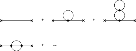
For example, the Feynman graphs up to the second order for two point function in theory become FIG. 1.
Figure 1: Feynman graphs for theory
We notice that there are no bubble graphs and it is useful to define the generating functional
(38)
We come to compare with the generating functional
in quantum field theory,
(39)
In the perturbation theory, this becomes,
(40)
where denotes that the contraction
is done by in the perturbation theory. In the previous section, we have shown that the expectation
value of n-point function in our theory and that in quantum theory
are equal, and thus the expectation value of any function in both theories
are equal. Therefore
(41)
Thus we have shown that our approach is equivalent with the quantum field theory in the perturbation level.
IV complex scalar, fermion, and gauge field
We can straightforwardly generalize our construction to the theory with complex scalar, fermion and gauge fields. From the previous sections,
once we can construct the Feynman propagators with using the
Gaussian noises, the perturbation theory of our approach is equivalent with
the perturbation theory of quantum field theory.
A free complex scalar field is composed with two real scalar fields, and , i.e. , and we introduce two complex Gaussian noises, and . We take
(42)
(43)
Since is the complex conjugate of , we may naively take . However this does not recover the Feynman propagator, but we should take
. Then,
(44)
(45)
(46)
(47)
Taking the average, we obtain
(48)
(49)
For the interacting theory, the equations which and
should satisfy are,
(50)
(51)
We take (44) and (45) as the zero-th order solutions and solve these equations perturbatically. Then as in the previous section, the n-point function in our approach is the same as that in quantum field theory.
For a Dirac fermion field , we introduce complex Gaussian distributions and and further introduce the Grassmann numbers, and the conjugate in order to realize the anti-commutation. We then combine these into and ,
(52)
(53)
where we do not take summation over the spin index .
We define and as
(54)
(55)
where
is the Feynman propagator for a Dirac fermion,
(56)
We now have the Grassmann numbers and , thus
the computation of expectation values should be modified,
(57)
(58)
Then we compute the expectation values and obtain
(59)
(60)
In the interacting theory, the Dirac fermion should satisfy
(61)
(62)
For a gauge field , we start with the action with the ghost and ,
(63)
where is the gauge index and is the gauge fixing parameter.
We take
the gauge field,
(64)
where is a complex Gaussian distribution and
so that
. transforms as adjoint and vector under the gauge and Lorentz transformations.
The expectation value of 2-point function then recovers the Feynman propagator,
(65)
The and fields take
(66)
(67)
where the summation is not taken over the index , but is taken over the index , is the Feynman propagator, is a complex Gaussian distribution and and are real Grassmann numbers. We obtain
(68)
We thus have recovered the Feynman propagators for complex scalar field, Dirac fermion, and gauge fields using Gaussian distributions.
V Summary and Discussion
We discussed a statistical theory which can compute the n-point function in quantum field theory in the perturbative level. The Gaussian noises which are introduced in our procedure are also needed in the stochasitic quantization Nelson:1966sp ; Parisi:1980ys ; Parisi:1983mgm ; Klauder:1983sp ; Damgaard:1987rr ; Namiki:1993fd . The difference from the stochastic quantization is that we do not need the fictitious time, but the similarity to the complex Langevin method is that we involve the complexification of the fields.
In quantum field theory, the perturbative expansion of qunatum field theory
suffers from various UV and/or IR divergences and the appropriate regularization methods, such as the UV cutoff and the dimensional regularization, and the renomalization are needed.
In our approach, we can apply the same regularization and renormalization
used in quantum field theory.
Acknowledgements.
The author would like to thank Bob Holdom and Feng-Li Lin for discussion.
References
(1)
T. H. Boyer,
“Random electrodynamics: The theory of classical electrodynamics with classical electromagnetic zero-point radiation,”
Phys. Rev. D 11 (1975), 790-808
doi:10.1103/PhysRevD.11.790
(2)
T. H. Boyer,
“General connection between random electrodynamics and quantum electrodynamics for free electromagnetic fields and for dipole oscillator systems,”
Phys. Rev. D 11 (1975), 809-830
doi:10.1103/PhysRevD.11.809
(3)
T. Hirayama and B. Holdom,
“Classical simulation of quantum fields. I.,”
Can. J. Phys. 84 (2006), 861
doi:10.1139/P06-083
[arXiv:hep-th/0507126 [hep-th]].
(4)
T. Hirayama, B. Holdom, R. Koniuk and T. Yavin,
“Classical simulation of quantum fields. II.,”
Can. J. Phys. 84 (2006), 879
doi:10.1139/P06-082
[arXiv:hep-lat/0507014 [hep-lat]].
(5)
B. Holdom,
“Approaching quantum behavior with classical fields,”
J. Phys. A 39 (2006), 7485-7500
doi:10.1088/0305-4470/39/23/021
[arXiv:hep-th/0602236 [hep-th]].
(6)
G. Aarts and J. Smit,
“Finiteness of hot classical scalar field theory and the plasmon damping rate,”
Phys. Lett. B 393 (1997), 395-402
doi:10.1016/S0370-2693(96)01624-3
[arXiv:hep-ph/9610415 [hep-ph]].
(7)
G. Aarts and J. Smit,
“Classical approximation for time dependent quantum field theory: Diagrammatic analysis for hot scalar fields,”
Nucl. Phys. B 511 (1998), 451-478
doi:10.1016/S0550-3213(97)00723-2
[arXiv:hep-ph/9707342 [hep-ph]].
(8)
C. Wetterich,
“Quantum particles from classical probabilities in phase space,”
[arXiv:1003.0772 [quant-ph]].
(9)
C. Wetterich,
“Quantum field theory from classical statistics,”
[arXiv:1111.4115 [hep-th]].
(10)
E. Nelson,
“Derivation of the Schrodinger equation from Newtonian mechanics,”
Phys. Rev. 150 (1966), 1079-1085
doi:10.1103/PhysRev.150.1079
(11)
G. Parisi and Y. s. Wu,
“Perturbation Theory Without Gauge Fixing,”
Sci. Sin. 24 (1981), 483
ASITP-80-004.
(12)
G. Parisi,
“ON COMPLEX PROBABILITIES,”
Phys. Lett. B 131 (1983), 393-395
doi:10.1016/0370-2693(83)90525-7
(13)
J. R. Klauder,
“Coherent State Langevin Equations for Canonical Quantum Systems With Applications to the Quantized Hall Effect,”
Phys. Rev. A 29 (1984), 2036-2047
doi:10.1103/PhysRevA.29.2036
(14)
P. H. Damgaard and H. Huffel,
“Stochastic Quantization,”
Phys. Rept. 152 (1987), 227
doi:10.1016/0370-1573(87)90144-X
(15)
M. Namiki,
“Basic ideas of stochastic quantization,”
Prog. Theor. Phys. Suppl. 111 (1993), 1-41
doi:10.1143/PTPS.111.1
(16)
G. Aarts, E. Seiler and I. O. Stamatescu,
“The Complex Langevin method: When can it be trusted?,”
Phys. Rev. D 81 (2010), 054508
doi:10.1103/PhysRevD.81.054508
[arXiv:0912.3360 [hep-lat]].
(17)
G. Aarts, F. A. James, E. Seiler and I. O. Stamatescu,
“Complex Langevin: Etiology and Diagnostics of its Main Problem,”
Eur. Phys. J. C 71 (2011), 1756
doi:10.1140/epjc/s10052-011-1756-5
[arXiv:1101.3270 [hep-lat]].
(18)
R. Anzaki, K. Fukushima, Y. Hidaka and T. Oka,
“Restricted phase-space approximation in real-time stochastic quantization,”
Annals Phys. 353 (2015), 107-128
doi:10.1016/j.aop.2014.11.004
[arXiv:1405.3154 [hep-ph]].
(19)
T. Ichihara, K. Nagata and K. Kashiwa,
“Test for a universal behavior of Dirac eigenvalues in the complex Langevin method,”
Phys. Rev. D 93 (2016) no.9, 094511
doi:10.1103/PhysRevD.93.094511
[arXiv:1603.09554 [hep-lat]].
(20)
G. Aarts, E. Seiler, D. Sexty and I. O. Stamatescu,
“Complex Langevin dynamics and zeroes of the fermion determinant,”
JHEP 05 (2017), 044
[erratum: JHEP 01 (2018), 128]
doi:10.1007/JHEP05(2017)044
[arXiv:1701.02322 [hep-lat]].
(21)
H. Fujii, S. Kamata and Y. Kikukawa,
“Performance of Complex Langevin Simulation in 0+1 dimensional massive Thirring model at finite density,”
[arXiv:1710.08524 [hep-lat]].
(22)
K. Nagata, J. Nishimura and S. Shimasaki,
“Complex Langevin calculations in finite density QCD at large /T with the deformation technique,”
Phys. Rev. D 98 (2018) no.11, 114513
doi:10.1103/PhysRevD.98.114513
[arXiv:1805.03964 [hep-lat]].
(23)
M. Scherzer, E. Seiler, D. Sexty and I. O. Stamatescu,
“Complex Langevin and boundary terms,”
Phys. Rev. D 99 (2019) no.1, 014512
doi:10.1103/PhysRevD.99.014512
[arXiv:1808.05187 [hep-lat]].
(24)
J. B. Kogut and D. K. Sinclair,
“Applying Complex Langevin Simulations to Lattice QCD at Finite Density,”
Phys. Rev. D 100 (2019) no.5, 054512
doi:10.1103/PhysRevD.100.054512
[arXiv:1903.02622 [hep-lat]].
(25)
M. Scherzer, E. Seiler, D. Sexty and I. O. Stamatescu,
“Controlling Complex Langevin simulations of lattice models by boundary term analysis,”
Phys. Rev. D 101 (2020) no.1, 014501
doi:10.1103/PhysRevD.101.014501
[arXiv:1910.09427 [hep-lat]].
(26)
K. Yasue,
“Stochastic calculus of variations,”
Journal of Functional Analysis 3 (1981) 327
(27)
T. Koide and T. Kodama,
“Stochastic variational method as quantization scheme: Field quantization of the complex Klein–Gordon equation,”
PTEP 2015 (2015) no.9, 093A03
doi:10.1093/ptep/ptv127
[arXiv:1306.6922 [hep-th]].
(28)
T. Koide, T. Kodama and K. Tsushima,
“Stochastic Variational Method as a Quantization Scheme II: Quantization of Electromagnetic Fields,”
[arXiv:1406.6295 [hep-th]].