On generality of Starobinsky and Higgs inflation in the Jordan frame

Abstract

We revisit the problem of generality of Starobinsky and Higgs inflation. The known results obtained in the Einstein frame are generalized for the case of an arbitrary initial energy of the scalar field. These results are compared with the results obtained directly in the Jordan frame, which, to our knowledge, has not been thoroughly explored in the literature previously. We demonstrate that the qualitative picture of initial conditions zone in the $(\phi,\dot{\phi})$ plane, which leads to sufficient amount of inflation, is quite similar for both the frames in the case of Higgs inflation. For Starobinsky inflation, the conformal transformation between the frames relates the geometrical variables in the Jordan frame with the properties of an effective scalar field in the Einstein frame. We show that the transformation $(H,R)\to(\phi,\dot{\phi})$ is not regular everywhere, leading to some peculiarities in the zone of good initial conditions in the $(H,R)$ plane.

I Introduction

Recent progress in observations of CMB has led to significant constraints on the viable models of inflation Akrami:2018odb . Very popular models with reasonable physical motivations like the quadratic $\frac{1}{2}m^{2}\phi^{2}$ and the quartic $\lambda\phi^{4}$ potentials are now strongly disfavored. The absence of any detection of the primordial tensor modes leads to the conclusion that the inflaton potential should rather be shallow. Other possibilities include the case of $\lambda\phi^{4}$ potential with the inflaton field non-minimally coupled to the scalar curvature $R$ (this model allows us to consider the Standard Model Higgs field as the inflaton) or the absence of any fundamental scalar field at all, with inflation induced by the $R^{2}$ term in the gravitation Lagrangian (Starobinsky inflation starobinsky1980new .) Note that these two models allow conformal transformation of the metric into the Einstein frame where the action takes the form of the usual General Relativity action with a minimally coupled canonical scalar field (in the case of $R^{2}$ inflation this field is purely an effective one). The potential required is again a shallow potential. That is why a detailed analysis of the inflaton dynamics with shallow potentials has recently become very important. In particular, old classic results of initial conditions which yield sufficient amount of inflation (that is inflation with at least 60 e-foldings) should be re-examined for the case of shallow potentials. Recent works on this topic have already indicated certain important differences from the classic case of the massive quadratic potential. In particular, starting from Planckian initial energy, initial scalar field values that lie close to $\phi=0$ for the shallow potentials yield, in contrast to the case of the massive scalar field potential, sufficient amount of inflation.

The goal of the present paper is to study the generality of inflation while starting from an energy different from the Planckian one. It has already been remarked that the requirement of initial Planckian energy for models with asymptotically flat potentials leads to initial dominance of the kinetic term. This might be considered to be not so natural, if we believe in initial equipartition between the kinetic and the potential term Gorbunov:2014ewa . Starting from Planckian energy is even less reasonable in the case of Higgs and Starobinsky inflation – in both the models considered in the Jordan frame effective gravitational constant can change in time, and its present value and the value at the early stages of evolution of the Universe can differ by orders of magnitude. This means that the Planck scale, being inversely proportional to the effective gravitational constant, changes during the cosmological evolution and there is no reason to take its present value while describing the early Universe. We can alternatively use the Einstein frame for description of these inflationary models, where the Planck scale remains constant. However, the conformal transformation to the Einstein frame does not conserve the energy. Hence if we use the Einstein frame as an effective description of Higgs or Starobinsky inflation (considering the corresponding Jordan frames as the physical ones), initial energy may again have no connection with the present value of the Planckian energy, despite the fact that the latter is conserved in the Einstein frame.

Quadratic gravity was first addressed by Weyl in 1918 weyl1918gravitation , later reappearing in the 60s and 70s, for example in buchdahl1962gravitational ; Buchdahl:1983zz ; tomita1978anisotropic . After that it has been investigated by many Berkin:1991nb ; Gurovich:1979xg ; Cotsakis:1997ck ; Cotsakis:2007un ; cotsakis2008slice ; Barrow:2005qv ; Barrow:2006xb ; Barrow:2009gx ; Carloni:2007br ; Miritzis:2007yn ; Miritzis:2003eu , for a historical review see schmidt2007fourth . Starobinsky inflationary model is realized in the particular case of $R^{2}$ lagrangian starobinsky1980new . Also in this connection there is the Ruzmaikina, Ruzmaikin solution ruzmaikina1970quadratic .

On the other hand, in the context of inflation, analysis is usually carried out in the Einstein frame, see for instance Mishra:2018dtg . The intention of this present work is to have specific emphasis on the Jordan frame. This frame is considered as the physical one, and hence, the results obtained in the Jordan frame have more direct physical meaning. Moreover, if quadratic gravity could be considered as a low-energy approximation of some more general theory ( for a particular example of such theory, see Koshelev ), the initial conditions good for inflation should be attractors for dynamics in such a full theory which can be used to check its consistency. Since there is no a priori reason for this underlying general theory to have an Einstein frame description, it is important that the results for initial conditions to be presented in the Jordan frame. In the present paper we consider initial conditions leading to successful Starobinsky inflation (we choose 60 e-folds as a criterion for inflation to be successful) in the Einstein frame in section II as well as in the Jordan frame in section III before describing the correspondence between these two frames in section IV. Since the scalar field potential in the Einstein frame for Staroninsky inflation shares some common features with the scalar field potential in the Einstein frame for the Higgs inflation, it is reasonable to consider the same problem for the Higgs inflation also. We then discuss similarities and differences in the results obtained for these two popular models. Our results are concluded in section V.

II Starobinsky inflation in the Einstein frame

In the following we will be studying quadratic gravity given by the action

$$S_{J}=\int d^{4}x\sqrt{-g}\frac{m_{p}^{2}}{2}\left[R+\beta R^{2}\right]~{},$$ (1)

where $m_{p}=\frac{1}{\sqrt{8\pi G}}$ is the reduced Planck mass. Note that (1) is written in the Jordan frame which is usually considered to be the physical frame with metric $g_{ab}$, being used to obtain spatial distances and time lapses. On the other hand, following Barrow and Cotsakis Barrow:1988xh , the Einstein frame metric is conformally related to the Jordan frame metric as $\tilde{g}_{ab}=e^{\tilde{\phi}}g_{ab}=f^{\prime}g_{ab}$. The conformal factor $f^{\prime}$ stands for the derivative of the particular $f(R)$ with respect to the argument. While the Lagrangian given in (1) reduces in the isotropic cases to the corresponding $f(R)=R+\beta R^{2}$, $R$ being the Ricci scalar.

The intention is to analyse the initial conditions for inflation for zero spatial curvature case in the Jordan frame and compare the results obtained with those in the Einstein frame which have been found before (for instance in Mishra:2018dtg ). Action (1) in the Einstein frame is given by

$$S_{E}=\int d^{4}x\sqrt{-\tilde{g}}\,\frac{m_{p}^{2}}{2}\left[\tilde{R}-\frac{3}{2}\tilde{g}^{ab}\partial_{a}\tilde{\phi}\partial_{b}\tilde{\phi}-\tilde{V}(\tilde{\phi})\right]~{}.$$ (2)

We have

$$R=\frac{e^{\tilde{\phi}}-1}{2\beta}~{},$$ (3)

and the potential depends on the particular type of $f(R)$

$$\tilde{V}(\tilde{\phi})=\frac{Rf^{\prime}-f}{(f^{\prime})^{2}}~{},$$ (4)

which, for $f(R)=R+\beta R^{2}$, becomes

$$\tilde{V}(\tilde{\phi})=\frac{\left(1-e^{-\tilde{\phi}}\right)^{2}}{4\beta}~{}.$$ (5)

We also follow the same units chosen in Mishra:2018dtg , in order to obtain the canonical kinetic term in (9) as well as to keep the appropriate dimension of the scalar field by choosing

$$\tilde{\phi}=\frac{2}{\sqrt{6}}\frac{\phi}{m_{p}}~{},$$ (6)

and potential

$$V(\phi)=\frac{m_{p}^{2}}{2}\frac{1}{4\beta}\left[1-\exp\left(-\frac{2}{\sqrt{6}}\frac{\phi}{m_{p}}\right)\right]^{2}~{}.$$ (7)

By expressing $\beta$ in terms of the mass of the scalaron given by $m=1/\sqrt{6\beta}$, the potential takes the form

$$V(\phi)=\frac{3}{4}m^{2}m_{p}^{2}\left[1-\exp\left(-\frac{2}{\sqrt{6}}\frac{\phi}{m_{p}}\right)\right]^{2}~{},$$ (8)

which is shown in figure 1 to possess an asymptotically flat right wing suitable for inflation. The action in the Einstein frame takes the familiar form

$$S_{E}=\int d^{4}x\sqrt{-\tilde{g}}\left[\frac{m_{p}^{2}}{2}\tilde{R}-\frac{1}{2}\tilde{g}^{ab}\partial_{a}\phi\partial_{b}\phi-V(\phi)\right]~{},$$ (9)

which coincides with the action given by equation (61) of Mishra:2018dtg with $V(\phi)$ given by (8).

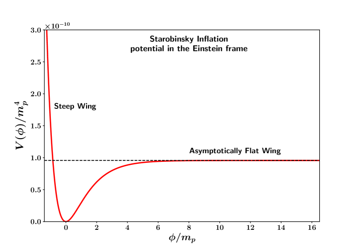
Figure 1: Starobinsky inflation potential in the Einstein frame (8) is shown in this figure to possess an asymptotically flat right wing and a steep left wing.

Analysis of generality of inflation for the action (9), thoroughly carried out in Mishra:2018dtg , leads to results rather different from the already known old results for a massive scalar field with $\frac{1}{2}m^{2}\phi^{2}$ potential. Initial conditions were chosen by keeping the initial energy of the scalar field to be of the order of Planckian energy, so that initial value of the scalar field $\phi$ fixes the initial value of $\dot{\phi}$ up to its sign. The central result of Mishra:2018dtg regarding the action (9) is that inflation is sufficient (with 60 or higher number of e-folds), if the initial $\phi\geq 15\,m_{p}$ for both possible signs of $\dot{\phi}$. More interesting is the fact that sufficient inflation can be achieved even starting from $\phi\geq-4\,m_{p}$ if we fix initial $\dot{\phi}$ to be positive. Note that it implies starting from initial $\phi=0$ with positive $\dot{\phi}$, we get enough inflation – a feature clearly different from the massive scalar field case.

Qualitatively this occurs because starting from $\phi=0$ the scalar field has enough kinetic energy to climb the shallow right wing of the potential in figure 1. This also means that if we consider similar potential, but possessing both left and right wings (this is the potential for Higgs inflation in the Einstein frame as shown in figure 2), then sufficient inflation can occur for any initial $\phi$, the only restriction being for $4\,m_{p}\leq|\phi|\leq 15\,m_{p}$, we would need $\mbox{sgn}(\dot{\phi})=\mbox{sgn}(\phi)$, while for $\phi$ outside this range the sign of initial $\dot{\phi}$ does not matter (see figure 16 of Mishra:2018dtg ).

Such striking difference between the power-law and the asymptotically flat potentials requires qualitative explanation. Since a symmetric potential is easier to study and it has its own significance being the Einstein frame potential for the Higgs inflation, we start our consideration from the symmetric potential before resuming the study of Starobinsky inflation in the Section III.

Generality of Higgs inflation revisited

The action for a scalar field $\varphi$ which couples non-minimally to gravity is given by higgs1 ; higgs2 ; kaiser ; Mishra:2018dtg

$$S_{J}=\int d^{4}x\sqrt{-g}\left[f(\varphi)R-\frac{1}{2}g^{ab}\partial_{a}\varphi\partial_{b}\varphi-U(\varphi)\right]$$ (10)

where $R$ is the Ricci scalar and $g_{ab}$ is the metric in the Jordan frame. The potential for the $SM$ Higgs field is given by

$$U(\varphi)=\frac{\lambda}{4}\left(\varphi^{2}-\sigma^{2}\right)^{2}$$ (11)

where $\sigma$ is the vacuum expectation value of the Higgs field

$$\sigma=246\,GeV=1.1\times 10^{-16}m_{p}$$ (12)

and the Higgs self-coupling constant has the value $\lambda=0.1$. Furthermore

$$f(\varphi)=\frac{1}{2}(m^{2}+\xi\varphi^{2})$$ (13)

where $m$ is a mass parameter given by kaiser

$$m^{2}=m_{p}^{2}-\xi\sigma^{2}$$

$\xi$ being the non-minimal coupling constant whose value

$$\xi=1.62\times 10^{4}$$ (14)

agrees with CMB observations Akrami:2018odb ; Mishra:2018dtg . For the above values of $\sigma$ and $\xi$, one finds $m\simeq m_{p}$, so that

$$f(\varphi)\simeq\frac{1}{2}(m_{p}^{2}+\xi\varphi^{2})=\frac{m_{p}^{2}}{2}\left(1+\frac{\xi\varphi^{2}}{m_{p}^{2}}\right)~{}.$$ (15)

We now transfer to the Einstein frame by means of the following conformal transformation of the metric Mishra:2018dtg

$$g_{ab}\longrightarrow\tilde{g}_{ab}=\Omega^{2}g_{ab}$$ (16)

where the conformal factor is given by

$$\Omega^{2}=\frac{2}{m_{p}^{2}}f(\varphi)=1+\frac{\xi\varphi^{2}}{m_{p}^{2}}~{}.$$ (17)

After the field redefinition $\varphi\longrightarrow\phi$ the action in the Einstein frame is given by Mishra:2018dtg

$$S_{E}=\int d^{4}x\sqrt{-\tilde{g}}\bigg{[}\frac{m_{p}^{2}}{2}\tilde{R}-\frac{1}{2}\tilde{g}^{ab}\partial_{a}\phi\partial_{b}\phi-V(\phi)\bigg{]}$$ (18)

where

$$V(\phi)=\frac{U[\varphi(\phi)]}{\Omega^{4}}$$ (19)

and

$$\frac{\partial\phi}{\partial\varphi}=\pm\frac{1}{\Omega^{2}}\sqrt{\Omega^{2}+\frac{6\xi^{2}\varphi^{2}}{m_{p}^{2}}}~{}.$$ (20)

Eq. (18) describes General Relativity (GR) in the presence of a minimally coupled scalar field $\phi$ with the potential $V(\phi)$. (The full derivation of the action in the Einstein frame is given in Mishra:2018dtg ; kaiser .)

While considering Higgs inflation in the Einstein frame, there is an approximate analytical form of the potential (19) given in Mishra:2018dtg which we reproduce here

$$V(\phi)\simeq V_{0}\left[1-\exp\left(-\frac{2}{\sqrt{6}}\frac{|\phi|}{m_{p}}\right)\right]^{2}~{},$$ (21)

where $V_{0}=\lambda m_{p}^{4}/(4\xi^{2})$. The symmetric potential potential (21) is shown in figure 2 to possess two asymptotically flat wings. We know from figure 16 in Mishra:2018dtg that the region near $\phi=0$ gives adequate amount of inflation in contrast to the massive scalar field case.

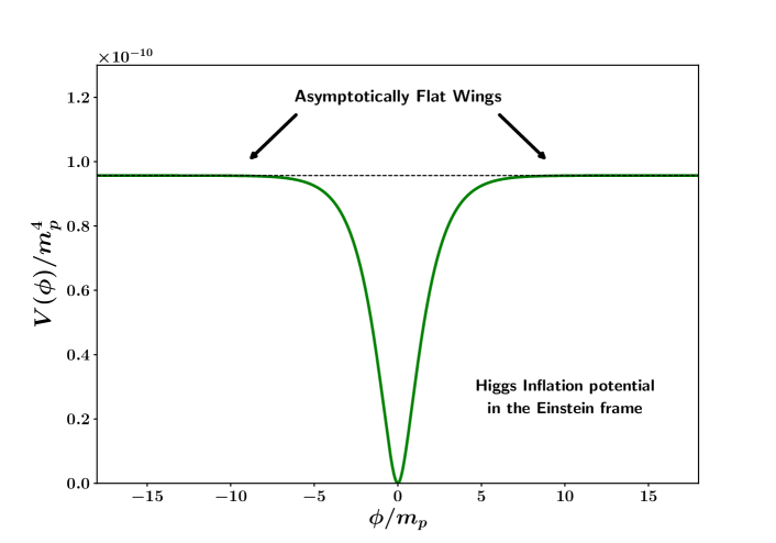
Figure 2: The symmetric Higgs inflation potential in the Einstein frame (21) is shown in this figure to possess two asymptotically flat wings.

II.1 The worst initial condition for inflation

We start our consideration by noting that, contrary to the wide-spread opinion, the $\phi=0$ initial condition is not the worst for inflation even for a massive scalar field case. To support this view let us consider the number of e-folds when starting from Planck energy for different initial $\phi$ (see figure 3 below) with the velocity of the scalar field is directed downward i.e $\mbox{sgn}(\dot{\phi})=-\mbox{sgn}(\phi)$. We can see clearly that $\phi=0$ initial condition is not the worst for inflation, though it indeed gives us insufficient number of e-foldings of inflation for $V(\phi)=\frac{1}{2}m^{2}\phi^{2}$ case. However, zero inflation corresponds to some finite value of initial $\phi$ at Planck scale given by $\phi_{i}\simeq 11~{}m_{p}$. Moreover, this value is roughly the same both for the massive and the asymptotically flat (21) potentials. The goal of the present subsection is to find this value analytically.

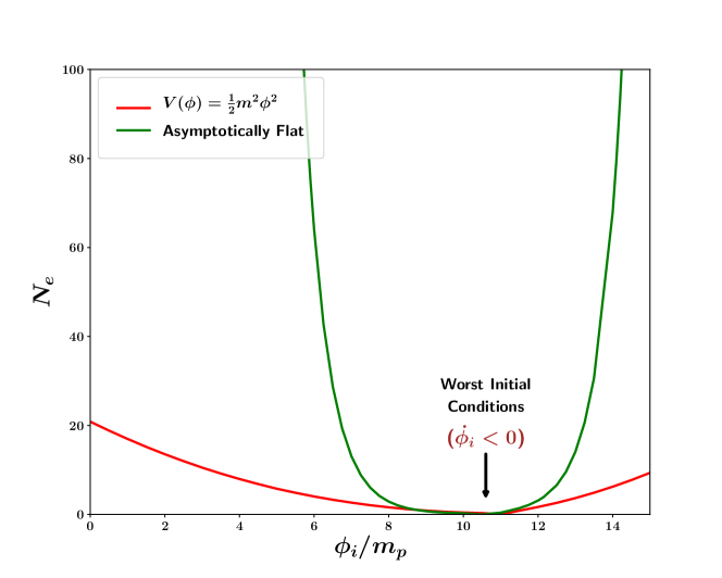
Figure 3: The number of e-foldings obtained before the end of inflation, estimated numerically, starting from the Planckian initial energy is plotted as a function of the initial field value $\phi_{i}$ with $\dot{\phi}_{i}<0$ for the case of massive quadratic potential $V(\phi)=\frac{1}{2}m^{2}\phi^{2}$ in red color and the asymptotically flat Higgs potential in the Einstein frame, given by (21), in green color. From this figure, it is clear that the worst initial conditions, leading to no inflation at all, lie near $\phi_{i}\simeq 11\,m_{p}$ for both type of potentials. The only difference is that if we start at $\phi_{i}=0$, the asymptotically flat potential leads to sufficient amount of inflation while the quadratic potential does not (which was the central result of Mishra:2018dtg ).

To do this we remind the reader another situation different from our problem here which, however, as we will show below, can be used to achieve our goal. Namely, consider the hypothetical case of contracting regime of the Universe filled with a scalar field. It is known that the equation of state $w_{\phi}$ has a different asymptote during contraction as compared to expansion. In particular, if the potential of the scalar field is less steep than the exponential one, the field is effectively massless during contraction for almost all initial conditions fixed at the beginning of the contraction stage FOSTER . This means that the effective equation of state is $w_{\phi}\simeq 1$, scale factor grows with time as $a\sim(t-t_{0})^{1/3}$, $H=1/3(t-t_{0})$, and the scalar field finally reaches the value

$$\phi_{b}=\frac{m_{p}}{12\pi}\ln{\frac{H_{b}}{H_{in}}},$$

where $H_{in}$ and $H_{b}$ are the Hubble parameters at the commencement and end of this regime $w_{\phi}\simeq 1$ after which universe starts expanding. For a massive scalar field, assuming that this regime ends at the Planck energy and remembering that it starts when scalar field is of the order of $m_{p}$ (for lower $\phi_{i}$ we have an amplifying oscillations on contraction stage), this formula can be rewritten as (see Sahni:2012er for details)

$$\phi_{b}=\frac{m_{p}}{12\pi}\ln{\frac{m_{p}}{m}}.$$ (22)

Note, that this formula is also applicable for a wider class of potentials. Namely, if the potential can be approximated as $m^{2}\phi^{2}/2$ for $\phi\leq m_{p}$, so that $w_{\phi}\approx 1$ regime starts when massive potential approximation is still valid, then scalar field will not feel the behaviour of its potential from $\phi\approx m_{p}$ till the Planck energy, because in this regime the potential is irrelevant. So that we can apply this formula for asymptotically flat potential of the Higgs inflation. Since this potential has the same effective mass in the small field limit as the observationally motivated $m$ for the massive scalar field potential, both the potentials lead to practically the same $\phi_{b}$ at the Planck boundary which is about $11\,m_{p}$.

Now we return to initial conditions which are the worst for inflation. To find an analytical answer let us consider the case of a contracting universe. A typical contracting universe has an equation of state of a stiff matter i.e $w_{\phi}\simeq 1$ as an attractor solution with the field growing fast while universe approaches the singularity. Now imagine that we stop the evolution at some energy level $H_{b}$ and reverse the direction of time. At this point, the field has climbed up to a value $\phi_{b}$ and has a velocity $\dot{\phi}_{b}$ of the order of the total energy, since the potential is negligible with respect to the kinetic term. After time reversal $\dot{\phi}$ changes its sign, and Universe will follow the same trajectory while expanding. Obviously, the equation of state is invariant under time reversal, so the universe will expand with no inflation at all. Hence the initial conditions $\phi=\phi_{b}$ and $\dot{\phi}=-\dot{\phi}_{b}$ are the worst initial conditions for inflation to occur. If we consider Planck boundary, $\dot{\phi}^{2}/2$ will be the Planck energy (since kinetic term dominates in this regime) and $\phi$ should be equal to $\phi_{b}$ which is found earlier. This coincides with the numerically obtained value of $\phi_{i}$ presented in figure 3. As it is known, $w=1$ at expansion (in contrast to contraction) requires a set of very special conditions, so for $\dot{\phi_{i}}$ different enough from the one constructed above, inflation becomes possible. These qualitative properties are true for both power-law as well as asymptotically flat potentials. However, for a massive scalar field on a Planckian boundary, $\phi=\phi_{b}=11\,m_{p}$ is not high enough to cause sufficient amount of inflation (i.e inflation with at least $60$ e-foldings) even if we start with $\dot{\phi_{i}}=0$. That is why the fact that the worst initial situation occurs for non-zero initial $\phi$ has a little effect for massive potential – this value is still close to zero from the viewpoint of adequate inflation. On the contrary, this value $\phi=\phi_{b}$ is high enough for successful inflation in the case of plateau potentials (8) and (21). However, large negative $\dot{\phi_{i}}$ kills the inflation completely, despite of the fact that initial $\phi$ is enough to get 60 e-folds when starting from $\dot{\phi_{i}}=0$. That is why the sign of initial $\dot{\phi}$ is more important for asymptotically flat potentials.

It is also worth mentioning that we can start from $\phi=0$ and with a Planckian kinetic energy in the massive scalar field case and get some number of e-foldings of inflation. Numerical simulations show that for $m\simeq 6\times 10^{-6}~{}m_{p}$, the field climbs till $\phi_{max}=10.4~{}m_{p}$ yielding about $28$ e-foldings. This is still not enough, however, it shows the effect of initial kinetic term in helping the field climb up the potential causing the universe to inflate even when starting from $\phi=0$. The same situation happens for an asymptotically flat potential and in this case, this effect is important for realistic models, because for a such potential, we can get adequate inflation with $N_{e}\geq 60$ starting from $\phi=0$.

Summarizing, in both the cases (massive and plateau potentials) initial $\phi=0$ leads to some e-foldings of inflation. While for plateau potentials, we do get sufficient amount of inflation, for a massive scalar field with the value of the scalar field mass that agrees with observation, inflation is not adequate. We have also checked numerically that for initial energy scale $H$ smaller than $10^{-3}~{}m_{p}$ we do not get adequate inflation from $\phi=0$ even for the case of plateau potentials (8) and (21), so that the structure of initial conditions zone good for inflation becomes similar to such zone for a massive scalar field. This means that the structure of the zone of “good” initial conditions for plateau potentials is rather sensitive to initial energy.

On the other hand, strictly zero inflation initial conditions necessarily require non-zero initial $\phi$. However, despite common general dynamical features, the set of initial conditions which leads to more than 60 e-folds starting from the Planck boundary looks quite different in the power-law potentials as compared to plateau potentials, as it have been shown in Mishra:2018dtg .

II.2 Initial conditions with arbitrary initial energy scale

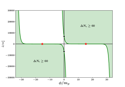
Figure 4: Above figure represents the basin of initial conditions for (a) $V(\phi)=\frac{1}{2}m^{2}\phi^{2}$ potential and (b) the Higgs inflation potential in the Einstein frame (21). The green regions contain initial conditions leading to sufficient amount of inflation with at least 60 e-foldings. The initial energy needed can be roughly characterized by black and red points in the plots – the black points indicate the least possible value of initial $\dot{\phi}$ required for sufficient inflation to occur starting from initial $\phi=0$, while the red points indicate the least initial value of $\phi$ for sufficient inflation to occur starting from initial $\dot{\phi}=0$.

The results of the previous subsection have been obtained for an initial energy of the order of Planck scale. They become even more clear if we construct initial conditions leading to at least 60 e-folds in the ($\phi$, $\dot{\phi}$) plane without fixing the initial energy scale $\rho_{\phi}$. Our results are presented in figure 4 for the massive $\frac{1}{2}m^{2}\phi^{2}$ potential in the left panel and for the asymptotically flat Higgs potential (21) in the Einstein frame. We can see that the results are qualitatively the same – the initial conditions located within the white bands in figure 4 $(a)$ and figure 4 $(b)$ do not lead to successful inflation. The only difference between these two figures is the width of this band, and this difference is responsible for the above mentioned fact that initial $\phi=0$ yields enough inflation in the case of plateau-like potentials, but not in the case of power-law potentials. Hence this difference appears, not because of some fundamental mathematical features of inflationary dynamics in these two cases, but rather due to the particular physical restrictions – starting within Planck energy ($\rho_{\phi}=m_{p}^{4}$) and demanding at least 60 e-folds.

It should be noted that starting from Planckian energy is a reasonable strategy if we consider the Einstein frame as a fundamental one. If, on the contrary, we think the Jordan frame to be the physical one, then taking into account that energy is not an invariant of the conformal transformation between the frames, there is no reason to fix the initial energy in the Einstein frame. From this point of view the results presented in figure 4 (b), where we did not fix the initial energy, are more relevant to the problem of generality of the Higgs inflation in the Einstein frame.

II.3 Higgs inflation in the Jordan frame

We work directly in the Jordan frame, considering the equations of motion Sami:2012uh obtained from the action (10), given by

$$\left(m_{p}^{2}+\xi\varphi^{2}\right)\left(2\dot{H}+3H^{2}\right)=-\frac{1}{2}\dot{\varphi}^{2}+U(\varphi)-4\xi H\varphi\dot{\varphi}-2\xi\left(\dot{\varphi}^{2}+\varphi\ddot{\varphi}\right)~{},$$ (23)

$$\ddot{\varphi}+3H\dot{\varphi}-\xi\varphi R+\frac{dU(\varphi)}{d\varphi}=0~{},$$ (24)

where $R=6\left(2H^{2}+\dot{H}\right)$. The expression for Hubble parameter is

$$H^{2}=\frac{1}{3m_{p}^{2}}\left[\frac{1}{2}\dot{\varphi}^{2}+U(\varphi)-3\xi\left(2H\varphi\dot{\varphi}+H^{2}\varphi^{2}\right)\right]$$ (25)

In this case our results, represented in the right panel of figure 5, are qualitatively similar to the Einstein frame results in the right panel of figure 4.

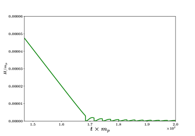
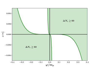
Figure 5: a) shows a typical inflationary trajectory in the Jordan frame of Higgs inflation (10). Note that $H$ decreases linearly during the inflationary stage and starts to oscillate after the end of inflation. The initial conditions basin is shown in b) where the black regions contain initial conditions leading to sufficient amount of Higgs inflation with at least 60 e-foldings in the Jordan frame.

III Starobinsky inflation in the Jordan frame

In this section we consider the problem of generality of Starobinsky inflation directly in the Jordan frame. The field equations resulting from action (1) are the following

$$E_{ab}\equiv G_{ab}+\beta H_{\>ab}^{(1)}=0\,,$$ (26)

where

$$G_{ab}=R_{ab}-\frac{1}{2}g_{ab}R\,,$$

$$H_{ab}^{(1)}=-\frac{1}{2}g_{ab}R^{2}+2RR_{ab}+2g_{ab}\nabla^{2}R-2R_{;ab}\,.$$ (27)

Let us emphasize that since the Einstein space $R_{ab}=g_{ab}\Lambda$ is an exact solution of (26), all vacuum solutions of GR are also exact solutions of the quadratic theory (1).

We choose the following line element

$$ds^{2}=-dt^{2}+a(t)^{2}d\vec{x}^{2},$$

such that the scale factor is $a(t)$ and the Hubble factor $H=\dot{a}/a$.

Note that time in the Jordan frame $dt$ and in the Einstein frame $d\tilde{t}$ are related as

$$dt=e^{-\tilde{\phi}/2}d\tilde{t}$$ (28)

In the zero spatial curvature case this choice allows us to write the field equations as

$$2\beta\ddot{H}H+6\beta\dot{H}H^{2}-\beta\dot{H}^{2}+\frac{1}{6}H^{2}=0$$ (29)

$$-12\beta\ddot{H}H-18\beta\dot{H}H^{2}-2\beta\dddot{H}-9\beta\dot{H}^{2}-\frac{1}{3}\dot{H}-\frac{1}{2}H^{2}=0,$$ (30)

the first of which is the constraint equation, while all the other field equations are identically satisfied.

Substitution of the expressions

$$R=6\dot{H}+12H^{2},\;\;\dot{R}=6\ddot{H}+24H\dot{H}$$ (31)

into the constraint equation (29) yields the expression for $H$ to be

$$H=\frac{-6\beta\dot{R}+\sqrt{36\beta^{2}\dot{R}^{2}+6\beta R^{2}(2\beta R+1)}}{6(2\beta R+1)}~{},$$ (32)

which is always positive for $\beta>0$ and $R>-1/(2\beta)$.

Before proceeding further, we must make few important remarks. Staying in the Jordan frame in the context of $f(R)$ theories, it is easy to see that the field equations given by (26) can be expressed as

$$f^{\prime}\left[R_{ab}-\frac{1}{2}Rg_{ab}\right]+\frac{1}{2}g_{ab}\left[Rf^{\prime}-f\right]-\nabla_{a}\nabla_{b}f^{\prime}+g_{ab}\square f^{\prime}=T^{\mbox{{\tiny M}}}_{ab}$$

$$f^{\prime}\left[R_{ab}-\frac{1}{2}Rg_{ab}\right]=T^{\mbox{{\tiny eff}}}_{ab},\;\;\rightarrow T^{\mbox{{\tiny eff}}}_{ab}=T^{\mbox{{\tiny M}}}_{ab}-\frac{1}{2}g_{ab}\left[Rf^{\prime}-f\right]+\nabla_{a}\nabla_{b}f^{\prime}-g_{ab}\square f^{\prime},$$

where $T^{\mbox{{\tiny eff}}}_{ab}$ is the effective behaviour of matter fields acting as source plus contributions from the scalar field and $f=R+\beta R^{2}$ as mentioned earlier. From these equations it follows that $f^{\prime}$ behaves as the inverse of gravitational constant. Looking at expression (3) it is possible to see that there is a minimum value for the Ricci scalar given by $R=-1/(2\beta)$. When $R=-1/(2\beta)$, $f^{\prime}$ is zero and physically, the gravitational constant diverges and so as all the perturbations. When $R<-1/(2\beta)$ gravity becomes repulsive, and the scalar field would then have a complicated dynamics, different from what is given by (9), the conformal factor between the Jordan-Einstein frames would then be given by $\tilde{g}_{ab}=f^{\prime}g_{ab}$ with $f^{\prime}<0$.

We now briefly remind the reader that for inflation in the Jordan frame, unlike in the Einstein frame, we do not have the usual quasi-de Sitter solution, rather the Ruzmaikin solution ruzmaikina1970quadratic which for the zero spatial curvature case is an asymptotic $t\rightarrow\infty$ isotropic solution with scale factor growing as

$$a(t)\propto\exp\left(-\frac{t^{2}}{72\beta}\right),$$ (33)

which gives a type of inflation

$$H=H_{0}-\frac{t}{36\beta},$$ (34)

with slow roll condition satisfied for $\beta>>1$.

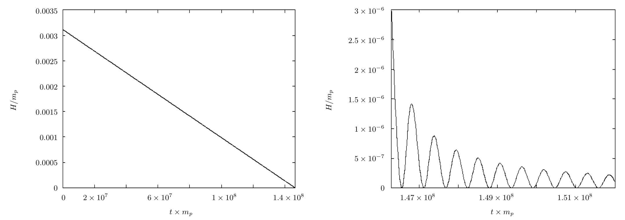
Figure 6: The time evolution of the Hubble parameter is shown for Starobinsky inflation in the Jordan frame. For an initial condition with $\beta=1.305\times 10^{9}~{}m_{p}^{-2}$ and, $H=1.0\times 10^{-5}~{}m_{p}$ and $\dot{H}=1.1\times 10^{-6}~{}m_{p}^{2}$, the left panel a) depicts Ruzmaikina Ruzmaikin solution (34), while the right panel b) shows the oscillatory regime after the end of inflation. The units are exactly the same as in the previous plot.

This solution is stable into the future. In this context a problem remains as how to halt inflation when $\beta<0$ . Also, when $\beta<0$ there is the tachyon. Otherwise, when $\beta>0$, the Hubble parameter linearly decreases $H\rightarrow 0$, and later oscillates as shown in figure 6.

Our numerical results for the generality of inflation have been presented in figure 7 where the region of initial conditions leading to sufficient amount of inflation has been marked in black. The left panel depicts the basin of initial conditions in the Jordan frame in terms of variables $(H,R)$. For comparison, the right panel represents the corresponding diagram for the Einstein frame in terms of variables $(\phi,\dot{\phi})$. Note that the boundary between initial conditions good for sufficient inflation (in black) and bad for sufficient inflation (white) is qualitatively the same as that in the case of Higgs inflation in the Einstein frame as shown in the right panel of figure 4. The only difference is that a second “good” region for inflation, present in the right panel of figure 4 is absent in the right panel of figure 7 due to the presence of the steep left branch of the effective potential (8) shown in figure 1 and hence the whole diagram is not symmetric with respect to changing the sign of $\phi$ and $\dot{\phi}$.

From figure 7, one can also notice the agreement between the Einstein and the Jordan frames. Particularly, an initial negative $\phi$ in the Einstein frame leads to sufficient inflation in the right panel. In the left panel, for the Jordan frame, the same negative initial $\phi$ corresponds to negative initial $R$, so the inflationary attractor extends itself to negative $R$ in the Jordan frame. However, a particular feature of the left panel plot seems to be contradictory to the picture in the Einstein frame. Namely, according to the left panel, one does not get sufficient amount of inflation starting from $R=0$ independent of the initial value of $H$. On the contrary, we know that inflationary trajectories, with adequate number of e-foldings, exist for initial $\phi=0$. Since zero $\phi$ corresponds to zero $R$, there seems to be an inconsistency. The goal of the next section is to resolve this apparent paradox.

IV Starobinsky Inflation: Comparison between the Jordan and the Einstein frame

We next turn to obtain the map of initial conditions in the Einstein frame to the corresponding initial conditions in the Jordan frame.

The expression for the Ricci scalar as well as equation (3) and its time derivative taken together with the constraint (29) give rise to

$$R=\frac{e^{\tilde{\phi}}-1}{2\beta}\rightarrow\dot{R}=\frac{\dot{\tilde{\phi}}e^{\tilde{\phi}}}{2\beta}$$ (35)

$$H=-\frac{1}{2}\dot{\tilde{\phi}}+\frac{\sqrt{6}e^{-\tilde{\phi}}}{12}\sqrt{\frac{e^{\tilde{\phi}}(6\dot{\tilde{\phi}}^{2}\beta e^{\tilde{\phi}}+e^{2\tilde{\phi}}-2e^{\tilde{\phi}}+1)}{\beta}}$$ (36)

$$\dot{H}=\frac{e^{\tilde{\phi}}-1}{12\beta}-2H^{2}$$ (37)

$$\ddot{H}=\frac{\dot{\tilde{\phi}}e^{\tilde{\phi}}}{12\beta}-4H\dot{H}~{}.$$ (38)

In the above mapping we have picked up the positive root $H>0$ which satisfies the constraint (29). Note that the expressions for higher derivatives in (37) and (38) follow from the definition of $H$ and $R$ in (35) and (36). While studying the generality of inflation, we either plot the initial conditions space in the $(R,H)$ plane directly or by specifying the initial values of $(\tilde{\phi},\dot{\tilde{\phi}})$ and then inserting into the expressions (35) and (36).

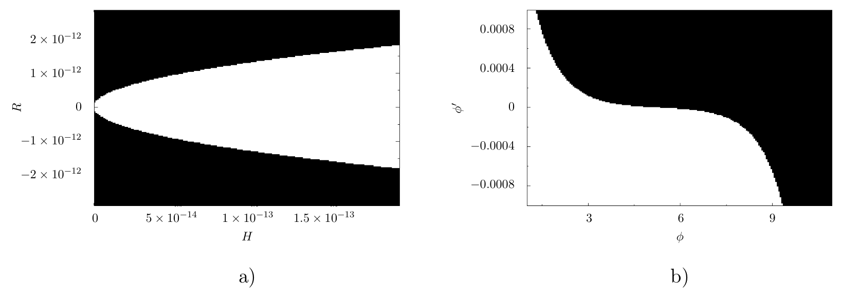
Figure 7: Initial conditions leading to sufficient inflation for Starobinsky inflation has been illustrated by the black color region. The left panel a) depicts the initial conditions basin directly in terms of ($H$,$R$) coordinates in the Jordan frame. While the right panel b) represents the same in the Einstein frame where we have chosen the variables $\phi$, $\phi^{\prime}$ with $\phi$ in units of $m_{p}$ and $\phi^{\prime}$ in units of $m_{p}^{2}$ given by (6). The value of $\beta$ is chosen to be $\beta=1.305\times 10^{9}$ in units of inverse square Planck mass, as required by CMB observations.

There is a indeterminacy in the value $H$ after fixing the $(\tilde{\phi},\dot{\tilde{\phi}})$ pair. Focusing on equation (36), it can be noticed that initial $\tilde{\phi}=0$ with $\dot{\tilde{\phi}}>0$ gives rise to vanishing initial value for $H=0$. This can be more clearly seen from the equation connecting Hubble parameter in both frames

$$\tilde{H}=\frac{\tilde{a}^{\prime}}{\tilde{a}}=e^{-\tilde{\phi}/2}\left(\frac{\dot{a}}{a}+\frac{\dot{\tilde{\phi}}}{2}\right)=\frac{\dot{\tilde{\phi}}/2+H}{\sqrt{2\beta R+1}}~{},$$ (39)

where the prime denotes, according to (28),

$$\tilde{\phi}^{\prime}=\frac{d}{d\tilde{t}}\tilde{\phi}=e^{-\tilde{\phi}/2}\frac{d}{dt}\tilde{\phi}=\frac{\dot{\tilde{\phi}}}{\sqrt{2\beta R+1}}~{}.$$

From the expressions (39) and (37), we conclude that the region of initial conditions with negligible value of the potential in the Einstein frame, for example near $\tilde{\phi}=0$ where $\tilde{H}\sim\dot{\tilde{\phi}}/2$, are mapped on to the origin of the $(H,R)$ plane in the Jordan frame.

The Jacobian of the map from $(\tilde{\phi},\dot{\tilde{\phi}})$ to $(H,R)$ region, as given in (35) and (36), is

$$J=\frac{e^{\tilde{\phi}}\left(\sqrt{\Delta}-\sqrt{6}e^{\tilde{\phi}}\dot{\tilde{\phi}}\right)}{4\beta\sqrt{\Delta}},$$ (40)

where

$$\Delta=\frac{e^{\tilde{\phi}}\left(6\dot{\tilde{\phi}}^{2}\beta e^{\tilde{\phi}}+e^{2\tilde{\phi}}-2e^{\tilde{\phi}}+1\right)}{\beta}.$$

From (40) it can be seen that the determinant $J$ of the map is zero for $\phi=0$ and $\dot{\phi}>0$, as expected from the above mentioned indeterminacy. Any initial value of $\dot{\tilde{\phi}}>0$ gets mapped on to the Jordan frame initial conditions $H=0,\;\dot{H}=0,\;\ddot{H}=\dot{\tilde{\phi}}/(12\beta)$. While the dynamical equation (30) says that the time evolution of this initial conditions with initial $\dddot{H}=0$ is well defined and it is non trivial. The set $(H,0)$ on the $(H,R)$ plane, corresponds to initial $\dot{\phi}<0$ and all such trajectories are clearly non-inflationary. This explains the apparent contradiction between numerical results of figure 7.

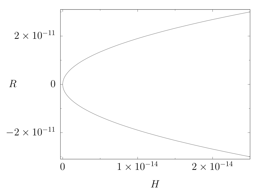
Figure 8: This figure is constructed with the same value of $\beta=1.305\times 10^{9}$ as used in figure 7. The trajectory in the ($H,~{}R$) space of the Jordan frame actually shows what happens when the Ricci scalar is negative initially. Any such trajectory would pass through the point $(0,0)$ in this plot.

In figure 8 we explicitly investigate the trajectories in which the Ricci scalar is negative initially. The conformal transformation between the Einstein and the Jordan frame only makes sense when $R>-1/(2\beta)$, which restricts the possible negative values of $R$ to a small region near the origin as shown in the right panel of figure 7. The trajectory in figure 8 in the ($H,~{}R$) space begins with an initial negative $R$, passes through $R=0$ and then grows to positive values of $R$, as expected from the correspondence between the Jordan and the Einstein frames. Besides that, figure 8 shows that the basin represented in figure 7 is an invariant set, as expected.

From figures 4 and 7 b), it is clear that figure 4 has two disjoints sets while in figure 7 there is only one set. The reason for this is the fact that the potential in the Einstein frame for the particular gravitational theory given by the action (1) is very steep for large negative values of $\phi$ which does not support inflationary trajectory FOSTER . While the potential for Higgs inflation is symmetric for $\phi\leftrightarrow-\phi$ Mishra:2018dtg so that inflation can occur for both positive and negative values of $\phi$. On the other hand, it is also possible to see that the upper right part of figure 4 b) is qualitatively reproduced in figure 7 b) as it should be, since both potentials (8) and (21) have the same behaviour for positive $\phi$.

V Conclusions

In the present paper we have considered the generality of Starobinsky inflation both in the Jordan as well as Einstein frame. The latter case has been considered in Mishra:2018dtg for a rather standard set up where the initial energy of the effective scalar field is fixed and usually chosen to be the Planck boundary. It has been argued in Gorbunov:2014ewa that this choice, being physically motivated for a fundamental scalar field, may not be very natural for an effective field. That is why we have lifted this requirement and analysed the two dimensional set of initial conditions in the phase space $(\phi,\dot{\phi})$. Due to similarity of potentials for Starobinsky and Higgs inflation we obtain results for generality of Higgs inflation as well. By giving up fixing the initial energy, have allowed ourselves to explain the nature of differences in the space of initial conditions leading to sufficient amount of inflation for massive and plateau potentials, as remarked in Mishra:2018dtg . The most striking example of this difference is the fact that initial field values close to $\phi=0$ can lead to sufficient inflation for a plateau potential, which is not the case for a massive scalar field potential. We show that this difference originates from the physical requirement of the initial energy, not from any mathematical properties of the equations of motion. When we allow initial energy not to be fixed, the resulting diagrams of initial conditions yielding sufficient inflation have similar form for both plateau and massive potentials.

We have also constructed diagrams of initial conditions leading to sufficient Starobinsky inflation in the Jordan frame, using the variables $(H,R)$. The mapping $(\phi,\dot{\phi})\to(H,R)$ appears to be singular for $\phi=0$, which leads to inaccessibility of inflation starting from initial $R=0$ despite the fact that $R=0$ corresponds to $\phi=0$ in the Einstein frame where sufficient inflation is possible starting from $\phi=0$. This results in completely different shapes of the phase space of appropriate initial conditions for Starobinsky inflation in the $(H,R)$ plane (Jordan frame) as compared to that in the $(\phi,\dot{\phi})$ plane (Einstein frame). Note that this does not happen for Higgs inflation since the phase spaces of initial conditions have similar shapes for both the Einstein and Jordan frames.

References

- (1) Y. Akrami et al. [Planck Collaboration], “Planck 2018 results. X. Constraints on inflation,” [arXiv:1807.06211 [astro-ph.CO]].
- (2) A. A. Starobinsky, “A New Type of Isotropic Cosmological Models Without Singularity,” Phys. Lett. 91B, 99 (1980) [Adv. Ser. Astrophys. Cosmol. 3, 130 (1987)].
- (3) D. S. Gorbunov and A. G. Panin, “Are - and Higgs-inflations really unlikely?,” Phys. Lett. B 743, 79 (2015) [arXiv:1412.3407 [astro-ph.CO]].
- (4) H. Weyl, “Gravitation and electricity,” Sitzungsber. Preuss. Akad. Wiss. Berlin (Math. Phys. ) 1918, 465 (1918).
- (5) H. Buchdahl, “On the gravitational field equations arising from the square of the Gaussian curvature,” Il Nuovo Cimento Series 10 23 no. 1, (1962) 141-157.
- (6) H. A. Buchdahl, “Non-linear Lagrangians and cosmological theory,” Mon. Not. Roy. Astron. Soc. 150, 1 (1970).
- (7) K. Tomita, T. Azuma, and H. Nariai, “On anisotropic and homogeneous cosmological models in the renormalized theory of gravitation,” Progress of Theoretical Physics 60 no. 2, (1978) 403–413.
- (8) A. L. Berkin,e-Print: “Contribution of the Weyl tensor to R**2 inflation,” Phys. Rev. D 44, 1020 (1991).
- (9) V. T. Gurovich and A. A. Starobinsky, “Quantum Effects And Regular Cosmological Models,” Sov. Phys. JETP 50, 844 (1979) [Zh. Eksp. Teor. Fiz. 77, 1683 (1979)].
- (10) S. Cotsakis and J. Miritzis, “Proof of the cosmic no hair conjecture for quadratic homogeneous cosmologies,” Class. Quant. Grav. 15, 2795 (1998) [gr-qc/9712026].
- (11) S. Cotsakis and A. Tsokaros, “Asymptotics of flat, radiation universes in quadratic gravity,” Phys. Lett. B 651, 341 (2007) [gr-qc/0703043 [GR-QC]].
- (12) S. Cotsakis, “Slice energy in higher order gravity theories and conformal transformations,” Grav. Cosmol. 14, 176 (2008) [gr-qc/0408095].
- (13) J. D. Barrow and S. Hervik, “Anisotropically inflating universes,” Phys. Rev. D 73, 023007 (2006) [gr-qc/0511127].
- (14) J. D. Barrow and S. Hervik, “On the evolution of universes in quadratic theories of gravity,” Phys. Rev. D 74, 124017 (2006) [gr-qc/0610013].
- (15) J. D. Barrow and S. Hervik, “Simple Types of Anisotropic Inflation,” Phys. Rev. D 81, 023513 (2010) [arXiv:0911.3805 [gr-qc]].
- (16) S. Carloni, A. Troisi and P. K. S. Dunsby, “Some remarks on the dynamical systems approach to fourth order gravity,” Gen. Rel. Grav. 41, 1757 (2009) [arXiv:0706.0452 [gr-qc]].
- (17) J. Miritzis,e-Print: “Oscillatory behavior of closed isotropic models in second order gravity theory,” Gen. Rel. Grav. 41, 49 (2009) [arXiv:0708.1396 [gr-qc]].
- (18) J. Miritzis, “Dynamical system approach to FRW models in higher order gravity theories,” J. Math. Phys. 44, 3900 (2003) [gr-qc/0305062].
- (19) H. J. Schmidt, “Fourth order gravity: Equations, history, and applications to cosmology,” eConf C 0602061, 12 (2006) [Int. J. Geom. Meth. Mod. Phys. 4, 209 (2007)] [gr-qc/0602017].
- (20) T. Ruzmaikina and A. Ruzmaikin, “Quadratic Corrections to the Lagrangian Density of the Gravitational Field and the Singularity,” Sov. Phys. JETP 30 (1970) 372.
- (21) S. S. Mishra, V. Sahni and A. V. Toporensky, “Initial conditions for Inflation in an FRW Universe,” Phys. Rev. D 98, no.8, 083538 (2018) [arXiv:1801.04948 [gr-qc]].
- (22) Alexey S. Koshelev, K. Sravan Kumar, Alexei A. Starobinsky, arXiv 2005.09550
- (23) E. Elizalde, S. D. Odintsov, T. Paul and D. Sáez-Chillón Gómez, “Inflationary universe in gravity with antisymmetric tensor fields and their suppression during its evolution,” Phys. Rev. D 99, no. 6, 063506 (2019) [arXiv:1811.02960 [gr-qc]].
- (24) A. Alho, S. Carloni and C. Uggla, “On dynamical systems approaches and methods in cosmology,” JCAP 1608, 064 (2016) [arXiv:1607.05715 [gr-qc]].
- (25) J. D. Barrow and S. Cotsakis, “Inflation and the Conformal Structure of Higher Order Gravity Theories,” Phys. Lett. B 214, 515 (1988).
- (26) F. L. Bezrukov and M. Shaposhnikov, Phys. Lett. B 659, 703-706 (2008) [arXiv:0710.3755].
- (27) R. Fakir and W.G. Williams, Phys. Rev. D 41, 1783-1791 (1990).
- (28) D. I. Kaiser, Phys. Rev. D 81, 084044 (2010) [arXiv:1003.1159].
- (29) S. Foster, “Scalar field cosmological models with hard potential walls,” [gr-qc/9806113].
- (30) V. Sahni and A. Toporensky, “Cosmological Hysteresis and the Cyclic Universe,” Phys. Rev. D 85, 123542 (2012) [arXiv:1203.0395 [gr-qc]]
- (31) M. Sami, M. Shahalam, M. Skugoreva and A. Toporensky, “Cosmological dynamics of non-minimally coupled scalar field system and its late time cosmic relevance,” Phys. Rev. D 86, 103532 (2012) [arXiv:1207.6691 [hep-th]].