Lift induced by slip inhomogeneities in lubricated contacts

Abstract

Lubrication forces depend to a high degree on elasticity, texture, charge, chemistry, and temperature of the interacting surfaces. Therefore, by appropriately designing surface properties, we may tailor lubrication forces to reduce friction, adhesion and wear between sliding surfaces or control repulsion, assembly, and collision of interacting particles. Here, we show that variations of slippage on one of the contacting surfaces induce a lift force. We demonstrate the consequences of this force on the mobility of a cylinder traveling near a wall and show the emergence of particle oscillation and migration that would not otherwise occur in the Stokes flow regime. Our study has implications for understanding how inhomogeneous biological interfaces interact with their environment; it also reveals a new method of patterning surfaces for controlling the motion of nearby particles.

In many physical processes, the flow of small particles such as cells, colloids, bubbles, grains, and fibers occurs near soft, porous and rough walls. The induced lubrication forces Reynolds (1886) on these particles depend on the elasticity, texture, and chemistry of the nearby wall. These forces may dominate over both bulk (e.g. Stokes drag) and surface (e.g. van der Waals and electrostatic) forces, and therefore determine single-particle motion and collective behavior.

The simplest configuration to characterize hydrodynamic particle-wall forces is that of an infinitely long circular cylinder traveling parallel to a rigid flat wall. At low Reynolds numbers, a rigid cylinder will experience zero wall-normal (lift) force and therefore move at a constant distance from the wall Jeffery and Onishi (1981). This is due to the time-reversal symmetry of the Stokes equations. However, if one of the interacting surfaces is soft, the moving particle will be repelled from the wall Sekimoto and Leibler (1993) as a result of the broken symmetry of the fluid pressure in the thin gap Cantat and Misbah (1999); Abkarian et al. (2002); Beaucourt et al. (2004); Skotheim and Mahadevan (2004); Urzay et al. (2007); Snoeijer et al. (2013). This elastohydrodynamic lift mechanism increases the gap thickness and reduces wear and friction between the siding surfaces Saintyves et al. (2016); Rallabandi et al. (2018); Vialar et al. (2019). It underlies exotic particle trajectories such as oscillations, Magnus-like effect, stick-slip motion, and spinning Salez and Mahadevan (2015); Rallabandi et al. (2017). Soft lubrication also underpins surface rheology Steinberger et al. (2008); Leroy et al. (2012); Wang et al. (2017) that is used to characterize the viscoelasticity of complex surfaces.

Besides softness, another ubiquitous feature of surfaces in biology and technology is surface inhomogeneities. For example, the surface of a Janus particle is divided into two halves with different chemistry (hydrophobic/hydrophilic) or texture (rough/smooth). This provides the particle with unique capabilities including self-assembly into complex structures Yan et al. (2012) and self-propulsion Golestanian et al. (2005). More generally, interfaces in living tissues (cell walls, blood vessels, cartilage, epithelia) vary in chemical and mechanical composition due to inhomogeneous distribution of cells and proteins. In technological applications, inhomogeneous surfaces arise as a consequence of manufacturing imperfections and wear, but also from surface patterning to control liquid transport Wexler et al. (2015) or heat transfer Attinger et al. (2014). Despite this ubiquity, there has been no investigation of the full set of lubrication forces arising from particle-wall interaction when the properties of one of the contacting surfaces vary.

In this Letter, we study lubrication forces when slippage Lauga et al. (2007) properties change along the contacting surfaces. We consider a model of spatially varying slip length $\ell$ at either the surface of a flat wall or the surface of a cylinder (Fig. 1a,b). Here, $\ell$ is defined as an effective property of the interface at some coarse-grained level. The slip length can be considered as a mesoscopic model emerging from small-scale features such as surface charges Bocquet and Barrat (2007), wall roughness Lacis and Bagheri (2017), superhydrophobicity Rothstein (2010), liquid infusion Wong et al. (2011), and temperature or solute concentration gradients Anderson (1989); Ajdari and Bocquet (2006).

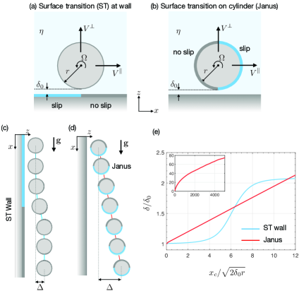
Figure 1: Two lubrication models. (a) 2D solid cylinder moving near a flat wall with a transition from a slip (blue) to a no slip (grey). (b) 2D cylinder half-coated with a slip region and moving near a wall. (c),(d) Sketches of cylinder trajectories for the two systems placed in a gravity field with $\delta_{0}=0.05r$, $\ell=1.79\delta_{0}$ and cylinder density $\rho_{\textrm{c}}=10\rho$. The particle experiences a small rotation that is not visually observable in (c) and (d).

(e) Normalized gap thickness versus the normalized transverse displacement of the cylinder. Inset shows the trajectory of the Janus cylinder over a larger spatial extent.

Using analytical and numerical treatments, we demonstrate that surface inhomogeneities give rise to particle trajectories such as oscillations, migration and propulsion. Underlying these phenomena is a normal lift force that arises from spatial variations in surface slippage. To illustrate this, consider the two configurations in Fig. 1(c,d). Both cases involve a cylinder of radius $r$ located a distance $\delta_{0}$ from a flat wall and immersed in a fluid with viscosity $\eta$ and density $\rho$. We assume small Reynolds number, $Re=\rho Vr/\eta\ll 1$, where $V$ is the characteristic velocity of the cylinder.

Figure 1(e) (blue) shows the trajectory of the cylinder falling freely under gravity next to a wall that has a single slip transition. The trajectory is obtained from numerical simulations of Stokes equations coupled to Newton’s equation of motion for the cylinder (see SI). As the cylinder passes the transition line, it migrates away from the wall a distance $\Delta$, that is comparable to $\delta_{0}$. In contrast, a wall with homogeneous slippage produces zero lift force (and consequently no wall-normal motion) on a cylinder Kaynan and Yariv (2017). Therefore, the lift arises here from the sudden change in slip length at the wall. By carrying out an expansion in the dimensionless slip length $L=\ell/\delta_{0}$, we will show that the lift force per unit length of the cylinder scales as $F_{z}\sim\eta V^{\parallel}\varepsilon^{-1}L$ at the transition line, and that $\Delta\sim\ell$, where $\varepsilon=\delta_{0}/r\ll 1$. Importantly, this lift force can be comparable in magnitude to other lubrication forces. As an example, for a red blood cell traveling near glycocalyx , variations of the slip length as small as a few nanometers induce a lift force comparable to the elastohydrodynamic one ($\sim 0.1$ pN) caused by glycocalyx deformation Davies et al. (2018).

Figure 1(e) (red) shows the trajectory (obtained from numerical simulations, see SI) of a Janus cylinder falling near a flat wall (Fig. 1d). We observe a persistent normal drift along the trajectory, since the transition from slip to no-slip is now located on the traveling cylinder itself thus constantly inducing a wall-normal force. Scaling estimates, that will be obtained below, indicate that $\Delta\sim x_{c}\ell/l_{\textrm{c}}$, where $l_{\textrm{c}}=\sqrt{2\delta_{0}r}$ is the lubrication contact length and $x_{c}$ is the transverse displacement. As $\Delta$ becomes larger than $r$, one expects a saturation of normal migration, since lubrication forces become negligible in the bulk. Nevertheless, as shown in the inset of Fig. 1(e), the effect holds for $\delta$ substantially larger than $r$.

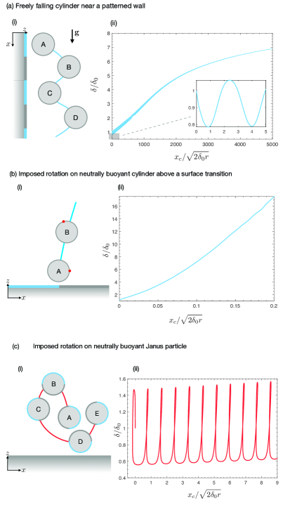
Figure 2: Cylinder trajectories induced by variation of slippage. (a) Cylinder falling near a wall that alternates between slip (blue) and no slip (grey). (b) Neutrally buoyant cylinder rotating above a slip-to-no-slip transition. (c) Neutrally buoyant Janus cylinder rotating next to a wall. Right column (ii) shows the normalized gap thickness as a function of the normalized transverse displacement. For all configurations, $\delta_{0}/r=0.05$ and $L=1.79$.

The coupling of rigid-body motion to slippage inhomogeneities can result in unexpected particle dynamics (Fig. 2). In the following, we will study in detail these motions using lubrication theory and scaling laws. At low Reynolds numbers, the force per unit length, $\textbf{F}=(F_{x},F_{z})$, and torque per unit length, $T$, on the cylinder are linearly related to the velocity $\textbf{V}=(V^{\parallel},V^{\bot})$ and the angular speed $\Omega$ of the cylinder. This is expressed by the symmetric resistance matrix Leal (2007),

$$\begin{bmatrix}F_{x}\\ F_{z}\\ T\end{bmatrix}=-\eta\begin{bmatrix}f_{x}^{\parallel}&-f_{x}^{\bot}&rf_{x}^{\omega}\\ -f_{z}^{\parallel}&f_{z}^{\bot}&-rf_{z}^{\omega}\\ rt^{\parallel}&-rt^{\bot}&r^{2}t^{\omega}\end{bmatrix}\begin{bmatrix}V^{\parallel}\\ V^{\bot}\\ \Omega\end{bmatrix},$$ (1)

where $f_{x}^{\bot}=f_{z}^{\parallel}$, $t^{\parallel}=f_{x}^{\omega}$ and $t^{\bot}=f_{z}^{\omega}$.

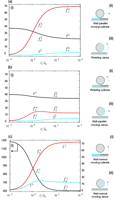
Figure 3: Analytical resistance coefficients for both model systems ($\varepsilon=0.05$). In the left column (i), the coefficients with no $\hat{}$ refer to configuration (ii) and the ones with $\hat{}$ refer to (iii).

Assuming a small gap, $\varepsilon=\delta_{0}/r\ll 1$, we explain below the procedure to determine the elements of the resistance matrix for the cylinder translating parallel to the wall with a slip-to-no-slip transition (Fig. 3a,ii).

We non-dimensionalize the variables as,

$$x =l_{\textrm{c}}\,X, z =\delta_{0}\,Z, h =\delta_{0}\,H,$$

$$u =V^{\parallel}\,U, w =\frac{\varepsilon^{1/2}V^{\parallel}}{\sqrt{2}}\,W, p =\frac{l_{\textrm{c}}\eta V^{\parallel}}{\delta_{0}^{2}}\,P,$$

where, $u,w$ are, respectively, the transverse and normal components of the fluid velocity, $p$ is the fluid excess pressure with respect to the atmospheric one. The cylinder surface is approximated as $h(x)=\delta_{0}+x^{2}/(2r)$. Inserting the dimensionless variables into the continuity and Stokes equations and neglecting $\mathcal{O}(\varepsilon)$ terms, we obtain

$$\partial_{X}P=\partial_{ZZ}U,\ \ \ \ \partial_{Z}P=0,\ \ \ \ \partial_{X}U+\partial_{Z}W=0.$$ (2)

In the laboratory frame of reference, the boundary conditions are,

$$\left.W\right|_{Z=0,H}=0,\qquad\left.U\right|_{Z=H}=1,$$ (3)

$$\left.U\right|_{Z=0}=\left.L\partial_{Z}U\right|_{Z=0}S.$$ (4)

Equation (4) accounts for slippage and is modelled through a Navier boundary condition. Moreover, $S$ equals one for $X<0$ and zero for $X>0$, where $X=0$ is the location of the transition from slip to no slip. The solution of Eqs. (2) and (4) is a combination of Couette and Poiseuille flows (see SI). From that solution, the fluid stress is projected onto the cylinder surface to obtain

$$f_{x}^{\parallel} =\sqrt{2}\varepsilon^{-1/2}\int_{-\infty}^{\infty}{\left(2XP+\partial_{Z}U\right)\textrm{d}X},$$ (5)

$$f_{z}^{\parallel} =2\varepsilon^{-1}\int_{-\infty}^{\infty}{P\textrm{d}X},$$ (6)

$$t^{\parallel} =\sqrt{2}\varepsilon^{-1/2}\int_{-\infty}^{\infty}{\partial_{Z}U\textrm{d}X}.$$ (7)

Figure 3(a,i) shows the elements (Eqs. 5-7) of the resistance matrix as a function of dimensionless slip length. When $\ell/\delta_{0}\rightarrow 0$, only the drag coefficient ($f_{x}^{\parallel}$) is non-zero, in agreement with the results for no slip surfaces Jeffery and Onishi (1981). For larger $\ell/\delta_{0}$, we note the emergence of non-zero elements related to lift force ($f_{z}^{\parallel}$) (as reported numerically in Fig. 1e) and torque $t^{\parallel}$.

Figure 3(b,i) shows the elements (denoted by the $\hat{}$ symbol) of a Janus cylinder that translates parallel to a wall. We again observe the emergence of off-diagonal terms of the resistance matrix for $\ell\approx\delta_{0}$; in particular the lift force ($\hat{f}_{z}^{\parallel}$) causing the constant normal migration shown in Fig. 1(e). The complete set of elements for both model systems is reported in Fig. 3. Note that due to the Lorentz reciprocal theorem Leal (2007) there is a symmetry between the two model systems.

To understand in detail the lift-induced mechanism of slip-to-no-slip transitions, we study the gap pressure distributions for three different slip lengths. Figure 4(a) shows the pressure distribution for a moving cylinder over an inhomogeneous wall (trajectory in Fig. 1c). The no-slip solution maintains an anti-symmetric pressure distribution (red). The introduction of a finite slip length breaks this symmetry (blue and black), as the gap pressure necessary to accelerate the flow through the gap (with varying thickness) is increased over the slippery section ($X<0$). Figure 4(b) shows the gap pressure of the wall-parallel moving Janus particle (trajectory in Fig. 1d). Here, the induced lubrication pressure needs to accommodate both for varying gap thickness and for varying fluid shear in the gap, which results in a pressure peak over the slippery section of the Janus cylinder. Note that due to the symmetry between the two configurations the pressure distributions in (a) and (b) are the mirror of distributions (c) and (d), respectively.

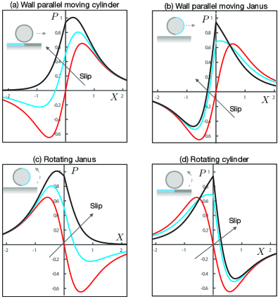
Figure 4: Lubrication pressure distributions in four configurations and for three slip lengths, $L=0$ (red), $L=1$ (blue) and $L=\infty$ (black).

We now explain the trajectories in Fig. 2 using the components of the resistance matrix shown in Fig. 3. In Fig. 2(a), a slip-to-no-slip transition pushes the cylinder away from the wall (Fig. 1c), whereas a no-slip-to-slip transition produces a negative $F_{z}$, pulling the cylinder towards the wall. The long-term net migration away from the wall (Fig. 2a,ii) is partially due to the fact that the push force is slightly larger than the pull force for each period due to different gap thicknesses during the pull and push events (see SI).

The second example involves a rotating neutrally buoyant cylinder (Fig. 2b). When the cylinder is released above a slippage transition on the wall, we observe a migration in both $x-$ and $z-$directions (see Fig. 2b,ii). The resistance coefficients in Fig. 3(b) and (c) explain this behavior. The imposed rotation produces a lift force ($F_{z}\sim\eta r\Omega f_{z}^{\omega}>0$) and a negative transverse thrust ($F_{x}\sim-\eta r\Omega f_{x}^{\omega}<0$). However, as the cylinder migrates away from the wall, we have $V^{\bot}>0$, which leads to a positive transverse thrust ($F_{x}\sim\eta V^{\bot}f_{x}^{\bot}>0$). The $V^{\bot}$-generated thrust dominates over the $\Omega$-generated thrust, such that the cylinder moves in the positive $x$ direction.

Table 1: Scaling laws for lift force ($F_{z}$) and wall-normal displacement ($\Delta$) for ST Wall or Janus particle. The imposed motion is either wall-parallel velocity or rotation. For the latter, the displacement shown is for one revolution.

	Motion	Lift force	Displacement
ST Wall	$V^{\parallel}$	$F_{z}\sim\eta V^{\parallel}\varepsilon^{-1}L$	$\Delta\sim\ell$
Janus	$V^{\parallel}$	$F_{z}\sim\eta V^{\parallel}\varepsilon^{-1}L$	$\Delta\sim\ell x_{\textrm{c}}/l_{\textrm{c}}$
ST Wall	$\Omega$	$F_{z}\sim\eta r\Omega\varepsilon^{-1}L$	$\Delta\sim\sqrt{r/\delta}\ell$
Janus	$\Omega$	$F_{z}\sim\eta r\Omega\varepsilon^{-1}L$	$\Delta\sim\ell\sqrt{r/\delta}-\frac{\ell\sqrt{r/\delta}}{\sqrt{1+\ell r^{1/2}\delta^{-3/2}}}$

The final example involves a rotating neutrally buoyant Janus cylinder (Fig. 2c). The cylinder undergoes a spiralling motion that results in positive transverse propulsion and positive wall-normal migration. We explain the motion in stages A-E depicted in Fig. 2(c). In stage $A$, the cylinder migrates upward since $\hat{f}_{z}^{\omega}>0$. It simultaneously migrates to the left since, due to the short exposure, $V^{\bot}$ is relatively small and we have $\lvert V^{\bot}\hat{f}_{x}^{\bot}\rvert<\lvert r\Omega\hat{f}_{x}^{\omega}\rvert$. In stage $B$, the Janus cylinder has rotated such that no slippage remains in the gap. Therefore, a lift force is no longer generated and the wall-normal drag force $\hat{f}_{z}^{\bot}$ hinders further upward migration. Stages $C$ and $D$ are the mirror of $A$ and $B$, respectively. Consequently, we observe a migration in the negative $z$ and positive $x$ directions. As the cylinder reaches stage $E$, it has experienced a net translation in the positive $x$ direction and a small net migration away from the wall from its initial position $A$. This is due to the difference in the magnitude of fluid stresses in the gap when slip ($B$) and no slip ($D$) surfaces face the wall.

Finally, we turn to scaling analysis to estimate the normal displacement induced by the lift force. We focus on the instant where a cylinder is located above the transition from slip to no slip on the wall (Fig. 1a). We assume no rotation, constant transverse and wall-normal velocities $V^{\parallel}$ and $V^{\perp}$, and negligible inertial effects (see SI). A wall-normal force balance yields $\eta f_{z}^{\parallel}V^{\parallel}=\eta f_{z}^{\bot}V^{\bot}$, corresponding to the magnitude of the lift and drag components, respectively. By carrying out an expansion in $L\ll 1$ of $f_{z}^{\parallel}$ and $f_{z}^{\bot}$, we can approximate the two coefficients using leading order terms as

$$f_{z}^{\parallel}\simeq 4\ell r/\delta_{0}^{2}\quad\mbox{and}\quad f_{z}^{\bot}\simeq-3\sqrt{2}\pi\left(\delta_{0}/r\right)^{-3/2}.$$ (8)

By assuming that the lift force approximately acts over $l_{\textrm{c}}$, we have

$$V^{\parallel}=l_{\textrm{c}}/\tau\qquad\mbox{and}\qquad V^{\bot}=\Delta/\tau,$$ (9)

where $\tau$ is the time it takes to traverse $l_{\textrm{c}}$, and $\Delta$ is the displacement from the wall. Inserting these estimates in the wall-normal force balance yields $\Delta\sim\ell$. This is in agreement with numerical results shown Fig. 1(c), where we observe $\Delta\approx\delta_{0}$ for $\ell\approx\delta_{0}$. For a Janus cylinder (Fig. 1b), there is no fixed time over which the displacement occurs, because the transition point travels along with the cylinder. Therefore, we expect a displacement $\sim\ell$ for each $l_{\textrm{c}}$ traversed. This yields,

$$\Delta\sim\ell x_{\textrm{c}}/l_{\textrm{c}},$$ (10)

where $x_{\textrm{c}}$ is the distance traversed along the wall. Table 1, summarizes the scaling estimates of the lift force and normal displacement, induced by transverse motion or rotation, for both systems in Fig. 1(a,b) (see SI).

To conclude, we have used a combination of numerical simulations, analytical results obtained from lubrication theory, and scaling arguments, to describe how fluid-immersed objects approaching contact with spatially inhomogeneous slippage properties may encounter non-trivial emergent forces and torques. In the presence of small slippage inhomogeneities, our scaling estimate suggests that the lift force, $F_{z,\textrm{slip}}$, has to be considered alongside other lubrication forces. For instance, using atomic-force microscopy, the elastohydrodynamic force was reported Zhang et al. (2020) to be $F_{z,\textrm{EHD}}\sim$$\text{\,}\mathrm{nN}$. Considering the same experimental setup, but with a rigid substrate exhibiting a $\sim 1$ $\text{\,}\mathrm{nm}$ slip inhomogeneity, we obtain $F_{z,\textrm{slip}}\sim$$\text{\,}\mathrm{nN}$, i.e. the same order of magnitude as for the soft substrate . Such slippage inhomogeneities may arise from small variations in surface preparation, localized defects, or cleaning processes. For example, in the experiments of a traveling Janus particle near a wall Ketzetzi et al. (2020), variations of contact angle up to 10^∘ on the same substrate were reported. Finally, our numerical results show how non-trivial particle trajectories can spontaneously emerge from slippage inhomogeneities. This opens up new interesting opportunities for the design of interfaces to control and influence nearby particle motion, as well as to reduce friction and wear. It also provides a foundation to explore more realistic situations found in nature and especially biology.