An accurate restarting for shift-and-invert Krylov subspaces
computing matrix exponential actions
of nonsymmetric matrices

Abstract

An accurate residual–time (AccuRT) restarting for computing matrix exponential actions of nonsymmetric matrices by the shift-and-invert (SAI) Krylov subspace method is proposed. The proposed restarting method is an extension of the recently proposed RT (residual–time) restarting and it is designed to avoid a possible accuracy loss in the conventional RT restarting. An expensive part of the SAI Krylov method is solution of linear systems with the shifted matrix. Since the AccuRT algorithm adjusts the shift value, we discuss how the proposed restarting can be implemented with just a single LU factorization (or a preconditioner setup) of the shifted matrix. Numerical experiments demonstrate an improved accuracy and efficiency of the approach.

Key words Shift-and-invert Krylov subspace methods; exponential time integration; Arnoldi method; Krylov subspace restarting

1 Introduction

Computing action of the matrix exponential on a given vector is a common task often occurring in various applications such as time integration [23], network analysis or model order reduction. If the matrix is large then Krylov subspace methods form an important group of methods that are well suited for this task [15]. Other methods for computing matrix exponential actions for large matrices include Chebyshev polynomials [4] and the scaling and squaring method combined with Taylor series [2]. Krylov subspace computations of the matrix exponential and other matrix functions has been an active research area, with many important developments such as rational Krylov subspace methods [31, 38, 11, 17, 18], restarting techniques [10, 37, 1, 14, 19, 26] and interesting large-scale computational applications [22, 11, 24, 5, 8].

Restarting techniques allow to keep the number Krylov basis vectors (i.e., the Krylov subspace dimension) bounded while trying to preserve convergence properties of the method. Recently proposed residual–time (RT) restarting for computing matrix exponential actions seems to be an attractive technique [9]. One of its advantages is that the RT-restarted polynomial Krylov subspace methods are guaranteed to converge to a required tolerance for any restart length [9]. Another nice feature of the RT restarting is that the size of the small projected problem which has to be solved in the course of iterations does not grow with each restart (as is the case for some other restarting methods, see e.g. [32, Chapter 3]). For instance, for a restart length 10 the Krylov subspace dimension and the size of the projected problem are at most 10. In addition, the projected problem in the RT-restarted Krylov subspace methods is evaluation of the matrix exponential of a small matrix (a projection of the original large matrix). This is a simple problem which can be efficiently carried out by one of the standard linear algebra techniques [16, 30, 20]. In contrast, the projected problem in the so-called residual-based restarting [10, 7] is a system of nonautonomous ordinary differential equations (ODEs), see [10, formula(3)]. Although this ODE system is small-sized, its solution is typically more costly and requires additional care, such as a proper choice of an ODE solver and its parameters.

An important class of rational Krylov subspace methods for the matrix exponential is shift-and-invert (SAI) Krylov subspace method [31, 38]. It often appears to be efficient in various applications because it requires solution of linear systems with a single shifted matrix only. One of the shortcomings of the RT restarting proposed in [9] is that the accuracy of the SAI Krylov method combined with RT restarting can not be guaranteed. This paper proposes an extension of the RT restarting for the SAI Krylov subspace method which is designed to attain a required accuracy. The proposed technique works for nonsymmetric matrices. Moreover, we show how to implement the proposed modification efficiently, so that an LU factorization or a preconditioner setup has to be carried out only once.

The paper is organized as follows. Our restarting technique, which we call AccuRT (accurate residual–time restarting) is described in Section 2. There we first give some background information on Krylov subspace methods (Section 2.1), then we introduce and analyze AccuRT (Section 2.2) and discuss how to organize solution of the shifted systems efficiently (Section 2.3). In Section 3 numerical experiments for two test problems are presented. Finally, we draw some conclusions in Section 4.

2 AccuRT: an accurate residual–time restarting

Let, unless indicated otherwise, $\|\cdot\|$ denote the 2-norm. Throughout the paper we assume that for $A\in\mathbb{R}^{n\times n}$ holds

$$\mathrm{Re}(x^{*}Ax)\geqslant 0,\qquad\forall x\in\mathbb{C}^{n},$$ (1)

where $\mathrm{Re}(z)$ denotes the real part of a complex number $z$.

2.1 Krylov subspace methods and RT restarting

Assume the matrix exponential action has to be computed for a given matrix $A\in\mathbb{R}^{n\times n}$, $v\in\mathbb{R}^{n}$ and $t>0$, i.e.,

$$\text{compute}\quad y:=\exp(-tA)v.$$ (2)

The problem is equivalent to solving initial value problem (IVP)

$$y^{\prime}(t)=-Ay(t),\quad y(0)=v,$$ (3)

where we slightly abuse the notation by using $t$ for both the independent variable in (3) and for time interval length in (2). Krylov subspace method for computing the matrix exponential action can be seen as a Galerkin projection of IVP (3) on the Krylov subspace

$$\mathcal{K}_{k}(A,v)=\mathrm{span}(v,Av,A^{2}v,\dots,A^{k-1}v).$$ (4)

First, an orthonormal basis of $\mathcal{K}_{k}(A,v)$ is computed by the standard Arnoldi (or, if $A=A^{T}$, by Lanczos) process [16, 33, 39, 34] and stored as the columns $v_{1}$, $v_{2}$, …, $v_{k}$ of a matrix $V_{k}=[v_{1}\dots v_{k}]\in\mathbb{R}^{n\times k}$, such that the following Arnoldi decomposition holds:

$$AV_{k}=V_{k+1}\underline{H}_{k}=V_{k}H_{k}+h_{k+1,k}v_{k+1}e_{k}^{T},$$ (5)

where $e_{k}=(0,\dots,0,1)^{T}\in\mathbb{R}^{k}$, $\underline{H}_{k}\in\mathbb{R}^{(k+1)\times k}$ is an upper Hessenberg matrix and $H_{k}\in\mathbb{R}^{k\times k}$ contains the first $k$ rows of $\underline{H}_{k}$. Then the Krylov subspace approximation $y_{k}(t)\approx\exp(-tA)v$ is defined as [13, 27, 21]

$$y_{k}(t)=V_{k}u(t),$$ (6)

where $u(t):\mathbb{R}\rightarrow\mathbb{R}^{k}$ solves IVP with the projected matrix $H_{k}=V_{k}^{T}AV_{k}$

$$u^{\prime}(t)=-H_{k}u(t),\quad u(0)=\beta e_{1}.$$ (7)

Here $\beta=\|v\|$ and $e_{1}=(1,0,\dots,0)^{T}\in\mathbb{R}^{k}$. Note that IVP (7) is a Galerkin projection of (3) on the Krylov subspace and that $u(t)$ can be computed as

$$u(t)=\exp(-tH_{k})\beta e_{1}.$$ (8)

If $k$ is not too large, (8) is a preferred way to compute $u$ which can be implemented by one of the standard dense linear algebra routines [20]. Computing $\exp(-tH_{k})$ is usually quicker than solving the ODE system in (7), which requires choosing a suitable ODE solver (e.g., stiff or non-stiff) and its parameters. Krylov subspace method (5)–(8) is sometimes called polynomial Krylov subspace method to emphasize the fact that vectors of the subspace (4) are polynomials in $A$.

A natural way of controlling the error of the Krylov subspace approximation (6) is to monitor the residual $r_{k}(t)$ of $y_{k}(t)$ with respect to the ODE $y^{\prime}=-Ay$, namely [10, 12, 7]

$$r_{k}(t)=-Ay_{k}(t)-y_{k}^{\prime}(t).$$ (9)

The residual is readily available in the course of the Arnoldi process computations as [10, 12, 7]

$$r_{k}(t)=-h_{k+1,k}(e_{k}^{T}u(t))v_{k+1},$$ (10)

where we see that $r_{k}(t)$ is a scalar function times $v_{k+1}$. Hence, $V_{k}^{T}r_{k}(t)=0$ for all $t$ and (6) is indeed a Galerkin projection on $\mathcal{K}_{k}(A,v)$. Some residual convergence results can be found, e.g., in [9].

Figure 1: A sketch of the RT restarting procedure, adopted from our paper [9]

The SAI (shift-and-invert) Krylov subspace method [31, 38] for computing (2) differs from the standard polynomial Krylov subspace method described above in that it builds the Krylov subspace for the shifted-and-inverted matrix $(I+\gamma A)^{-1}$ instead of $A$, with $\gamma>0$ being a fixed parameter. This is done to accelerate convergence: the Arnoldi process tends to emphasize the largest eigenvalues of $(I+\gamma A)^{-1}$ corresponding to the smallest eigenvalues of $A$. The latter are important for the exponential which is a quickly decaying function (assuming real arguments). The price to pay for this accelerated convergence is the necessity to solve a linear system with the matrix $I+\gamma A$ at each Krylov step. The Arnoldi decomposition (5) for the SAI matrix $(I+\gamma A)^{-1}$, i.e.,

$$(I+\gamma A)^{-1}V_{k}=V_{k+1}\underline{\tilde{H}}_{k}=V_{k}\tilde{H}_{k}+\tilde{h}_{k+1,k}v_{k+1}e_{k}^{T},$$

is more convenient to use in a transformed form

$$AV_{k}=V_{k}H_{k}-\frac{\tilde{h}_{k+1,k}}{\gamma}(I+\gamma A)v_{k+1}e_{k}^{T}\tilde{H}_{k}^{-1},$$ (11)

where the notation $\tilde{\cdot}$ is used to indicate that the projection is built for the SAI matrix $(I+\gamma A)^{-1}$ and $H_{k}$ is defined as the inverse SAI transformation

$$H_{k}=\frac{1}{\gamma}(\tilde{H}_{k}^{-1}-I).$$ (12)

Note that the matrices $V_{k+1}$ and $H_{k}$ here are different from those in (5). The SAI Krylov subspace method is analyzed, e.g., in [31, 38, 17].

In the SAI Krylov subspace method the residual can be easily computed as [7]

$$r_{k}(t)=\frac{\tilde{h}_{k+1,k}}{\gamma}(e_{k}^{T}\tilde{H}_{k}^{-1}u(t))\cdot(I+\gamma A)v_{k+1},$$ (13)

where $u(t)$ is the solution of the projected IVP (7), with $H_{k}$ being the back transformed SAI matrix (12).

The shift value $\gamma$ is usually chosen in accordance with the length $t$ of the time interval $[0,t]$, see [38]. A possible often used value is $\gamma=t/10$. Hence, changing $\gamma$ means changing $t$. The usual polynomial Krylov subspace method (5)–(8) has an attractive property that it is invariant of $t$: once $V_{k+1}$ and $\underline{H}_{k}$ are computed, they can be successfully used for any $t$ (although the quality of approximation $y_{k}(t)\approx y(t)$ does deteriorates with $t$). Unfortunately, this nice property is not fully shared by the SAI Krylov subspace method: its matrices $V_{k+1}$ and $\tilde{\underline{H}}_{k}$ do depend on $\gamma$ which, in turn, depends on $t$. However, in practice, one certainly can use the computed Arnoldi matrices $V_{k+1}$ and $\tilde{\underline{H}}_{k}$ for a certain range of $t$ without recomputing them.

Recently proposed RT (residual–time) restarting is based on the fact that the residual as a function of $t$ tends to be a non-decreasing function. Hence, once a maximum number $k_{\max}$ Krylov steps are done (so that storing and working with more Krylov basis vectors is too expensive), we can find a time subinterval $[0,\delta]$, $\delta<t$, where the residual norm is already sufficiently small. We can then restart the Krylov method by setting $v:=y_{k_{\max}}(\delta)$, decreasing the time interval $t:=t-\delta$ and performing the next $k_{\max}$ Krylov steps solving problem (2) with the modified $v$ and $t$. The RT restarting procedure is sketched in Figure 1.

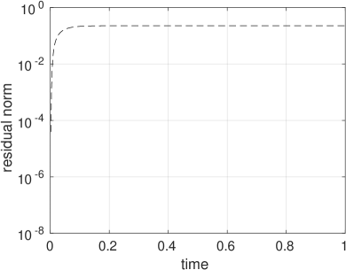
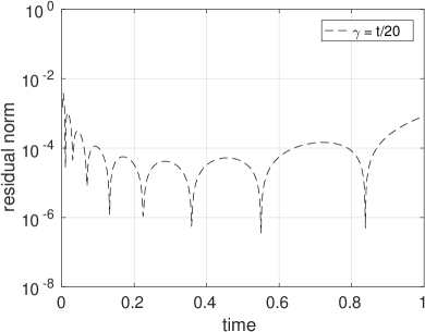
Figure 2: Residual norms $\|r_{k}(s)\|$ as functions of time $s\in[0,t]$, $t=1$, for the polynomial (left) and SAI (right) Krylov subspace methods, after $k=10$ Krylov steps. The SAI shift value is $\gamma=t/20$. The matrix $A$ is a discretized convection–diffusion operator for the Peclet number $\textit{P\!e}=200$ and $802\times 802$ grid (see Section 3.2 for more detail). For both plots the residual norm values are computed in 500 equidistant points in $[0,1]$.

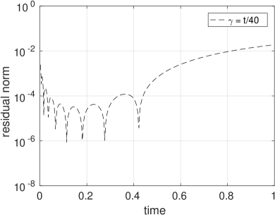
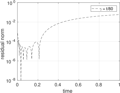
Figure 3: Residual norms $\|r_{k}(s)\|$ as functions of time $s\in[0,t]$, $t=1$, for the SAI Krylov subspace methods for $\gamma=t/40$ (left) and $\gamma=t/80$ (right), after $k=10$ Krylov steps. The matrix $A$ is a discretized convection–diffusion operator for the Peclet number $\textit{P\!e}=200$ and $802\times 802$ grid (see Section 3.2 for more detail). For both plots the residual norm values are computed in 500 equidistant points in $[0,1]$.

2.2 AccuRT ideas and algorithm

The residual as a function of $t$ in the SAI Krylov subspace method exhibits a much more irregular behavior than in the polynomial Krylov method (5)–(8), see Figure 2. If the RT restarting is applied for the SAI Krylov subspace method then it can happen that $\delta$ such that $\|r_{k}(s)\|$ is below a certain tolerance for $s\in[0,\delta]$ is too small to be used in practice for an efficient restarting. Of course, we could also restart by setting $\delta$ to any as large as possible point $s$ where $\|r_{k}(s)\|$ is small enough, cf. Figure 2. However, there is no guarantee that $\min_{s\in[0,t]}\|r_{k}(s)\|$ is within the required tolerance and, if this is the case, the restarting with any $\delta\in[0,t]$ inevitably leads to an accuracy loss.

Here we propose an approach to fix this failure of the RT restarting in the SAI Krylov subspace method. The approach is based on the following two simple observations.

1. Since $\gamma$ is usually chosen proportionally to $t$, taking a smaller shift value $\gamma$ effectively means a shorter time interval $[0,t]$. For nonsymmetric matrices $A$ the SAI Krylov residual $r_{k}(s)$ tends to become smaller in norm with smaller $\gamma$ on some time subinterval $s\in[0,\delta]$, $0<\delta<t$, see Figure 3.

2. As already noted, to change $\gamma$ in the SAI Krylov subspace method we have to carry out the whole Arnoldi process anew. However, once a shifted linear system with the matrix $I+\gamma A$ is solved for a certain shift $\gamma$, a part of the spent computational costs can be re-used for solving the shifted linear systems with a smaller shift $\tilde{\gamma}\leqslant\gamma$. In particular, if a (sparse) LU factorization is computed for a certain shift $\gamma$, it can be successfully used as a preconditioner for solving shifted systems with $I+\tilde{\gamma}A$, $\tilde{\gamma}\leqslant\gamma$ (see Proposition 2).

Based on these observations we propose to organize an improved RT restarting for the SAI Krylov subspace method as follows. Assume we can carry out at most $k_{\max}$ steps of the Arnoldi or Lanczos process, since storing (or working with) more than $k_{\max}$ Krylov basis vectors is too expensive. We perform $k=1,\dots,k_{\max}$ steps checking at each step the residual norm $\|r_{k}(t)\|$, cf. (13). If the residual norm turns out to be smaller than the required tolerance, we stop. Otherwise, after performing step $k=k_{\max}$, we analyze the function $\|r_{k}(s)\|$ for $s\in[0,t]$. If no point $s$ can be found where $\|r_{k}(s)\|$ is small enough, we decrease $\gamma$ by a factor of two and repeat $k=1,\dots,k_{\max}$ steps of the method. The restarting procedure (which is presented in detail in Figure 4) can be repeated until the residual norm is small enough at the end of the given time interval.

If a (sparse) LU factorization is prohibitively expensive, a preconditioned solver can be used to solve the shifted linear system. In the algorithm presented in Figure 4 we then replace the LU factorization step by a setup of the preconditioner. The computed preconditioner can then be used for all the shift values, i.e., it suffices to set up the preconditioner once. Note that the observed behavior of the SAI Krylov residual for decreasing $\gamma$ does not hold for symmetric $A$. This is reflected by a rather sharp estimate [38, Lemma 3.1] (in the estimate there, take $\mu=0$ and set $\gamma$ proportional to $t=\tau$).

The following lemma and proposition show that the residual $r_{k}(s)$ of the SAI Krylov subspace method is bounded in norm as a function of time. The way it is bounded depends on $\gamma$.

Lemma 1.

Let $A\in\mathbb{R}^{n\times n}$ be a matrix for which relation (1) holds and let $H_{k}$ be the matrix obtained in the SAI Krylov subspace method, see (11),(12). Then there exists a constant $\omega_{k}\geqslant 0$ such that

$$\|\exp(-tH_{k})\|\leqslant e^{-t\omega_{k}}.$$ (14)

Proof.

Let $\omega=\min_{x\in\mathbb{C}^{n},\|x\|=1}\mathrm{Re}(x^{*}Ax)$. It is well known (see, e.g., [25, Theorem 2.4]) that

$$\mathrm{Re}(x^{*}Ax)\geqslant\omega,\;\forall x\in\mathbb{C}^{n}\quad\Leftrightarrow\quad\|\exp(-tA)\|\leqslant e^{-t\omega}.$$

According to (1), these two equivalent relations hold with $\omega\geqslant 0$. Furthermore, these conditions are equivalent to [25, Theorem 2.13]

$$\|(I+\gamma A)^{-1}\|\leqslant\frac{1}{1+\gamma\omega},$$

which holds for all $\gamma>0$ and all $\omega\in\mathbb{R}$ provided that $1+\gamma\omega>0$. We assume $\gamma>0$, as is the case in the SAI Krylov subspace method. Let us define

$$\omega_{k}:=\frac{1}{\gamma}(\|\tilde{H}_{k}\|^{-1}-1),$$

so that $\|\tilde{H}_{k}\|=1/(1+\gamma\omega_{k})$. We have

$$\frac{1}{1+\gamma\omega_{k}}=\|\tilde{H}_{k}\|=\|V_{k}^{T}(I+\gamma A)^{-1}V_{k}\|\leqslant\|(I+\gamma A)^{-1}\|\leqslant\frac{1}{1+\gamma\omega},$$

from which it follows that $0\leqslant\omega\leqslant\omega_{k}$. Since $\tilde{H}_{k}=(I+\gamma H_{k})^{-1}$ (cf. (12)), we obtain, again using [25, Theorem 2.13],

$$\|(I+\gamma H_{k})^{-1}\|=\frac{1}{1+\gamma\omega_{k}}\leqslant\frac{1}{1+\gamma\omega}\quad\Leftrightarrow\quad\mathrm{Re}(x^{*}H_{k}x)\geqslant\omega_{k},\;\forall x\in\mathbb{C}^{k},$$ (15)

which is equivalent to inequality (14) we prove. ∎

Define function $\varphi(z)$ as (see, e.g., [23])

$$\varphi(z)=(e^{z}-1)/z.$$ (16)

Proposition 1.

Let $A\in\mathbb{R}^{n\times n}$ be a matrix for which relation (1) holds and let $r_{k}(t)$ be the residual of the SAI Krylov subspace method defined by (13), applied to solve problem (2). Then it holds for all $t\geqslant 0$

$$r_{k}(t) =\beta_{k}(t)\cdot w_{k+1},\quad\beta_{k}(t)=\frac{\tilde{h}_{k+1,k}}{\gamma}e_{k}^{T}(I+\gamma H_{k})u(t),\quad w_{k+1}=(I+\gamma A)v_{k+1},$$ (17)

$$\|r_{k}(t)\| =|\beta_{k}(t)|\,\|w_{k+1}\|,$$

$$|\beta_{k}(t)| \leqslant\beta\tilde{h}_{k+1,k}\left(\frac{1}{\gamma}\min\left\{t\|(I+\gamma H_{k})H_{k}\|\,\varphi(-t\omega_{k})\,,\,\|I+\gamma H_{k}\|(1+e^{-t\omega_{k}})\right\}\right.$$

$$\qquad\qquad\qquad\qquad\qquad\qquad\qquad\qquad\qquad\qquad\qquad\qquad\qquad+|h_{k,1}|\biggr{)}$$ (18)

where $u(t)$ is defined by (8),(12), $\omega_{k}\geqslant 0$ is the constant introduced in (14) and $\tilde{h}_{k+1,k}$ and $h_{k,1}$ are the corresponding entries of the matrices $\underline{\tilde{H}}_{k}\in\mathbb{R}^{(k+1)\times k}$ and $H_{k}\in\mathbb{R}^{k\times k}$, respectively (see (11),(12)). Here, the minimum is taken among the two elements of the set indicated by the braces $\{\dots\}$. Note that $\underline{\tilde{H}}_{k}$ in the estimate above depends on $\gamma$ (and, hence, so do $H_{k}$, $u(t)$, and $\omega_{k}$).

Proof.

Relation (17) is identical to (13) (cf. (12)), its proof can be found in [7]. Using (12),(7), we have

$$|\beta_{k}(0)| =\frac{\tilde{h}_{k+1,k}}{\gamma}|e_{k}^{T}\tilde{H}_{k}^{-1}u(0)|=\frac{\tilde{h}_{k+1,k}}{\gamma}|e_{k}^{T}(I+\gamma H_{k})\beta e_{1}|$$

$$=\tilde{h}_{k+1,k}|e_{k}^{T}H_{k}\beta e_{1}|=\beta\tilde{h}_{k+1,k}|h_{k,1}|.$$

Furthermore, it is not difficult to check that, cf. (16),

$$u(t)-u(0)=(\exp(-tH_{k})-I)u(0)=-tH_{k}\varphi(-tH_{k})u(0).$$

Therefore, with $u(0)=\beta e_{1}$ and $\tilde{H}_{k}^{-1}=I+\gamma H_{k}$, we can estimate

$$\|(I+\gamma H_{k})(u(t)-u(0)\|=t\|(I+\gamma H_{k})H_{k}\varphi(-tH_{k})u(0)\|$$ (19)

$$\leqslant t\|(I+\gamma H_{k})H_{k}\|\|\varphi(-tH_{k})\|\|u(0)\|\leqslant\beta t\|(I+\gamma H_{k})H_{k}\|\varphi(-t\omega_{k}).$$

Here we used an inequality

$$\|\varphi(-tH_{k})\|\leqslant\varphi(-t\omega_{k}),$$

which holds due to the property (14), (15), see, e.g., [23, proof of Lemma 2.4]. The estimate (19) is especially useful for small $t$. An alternative estimate, which may be sharper for large $t$, is

$$\|(I+\gamma H_{k})(u(t)-u(0)\|=\|(I+\gamma H_{k})(\exp(-tH_{k})-I)u(0)\|$$ (20)

$$\leqslant\|I+\gamma H_{k}\|\|\exp(-tH_{k})-I\|\|u(0)\|\leqslant\beta\|I+\gamma H_{k}\|(1+\|\exp(-tH_{k})\|)$$

$$\leqslant\beta\|I+\gamma H_{k}\|(1+e^{-t\omega_{k}}),$$

where the estimate (14) is used. From (19),(20) it follows that

$$\|(I+\gamma H_{k})(u(t)-u(0)\|\leqslant\beta\min\left\{t\|(I+\gamma H_{k})H_{k}\|\varphi(-t\omega_{k}),\|I+\gamma H_{k}\|(1+e^{-t\omega_{k}})\right\}.$$

We can then estimate

$$|\beta_{k}(t)|\leqslant|\beta_{k}(t)-\beta_{k}(0)|+|\beta_{k}(0)|$$

$$=\frac{\tilde{h}_{k+1,k}}{\gamma}|e_{k}^{T}(I+\gamma H_{k})(u(t)-u(0))|+\beta\tilde{h}_{k+1,k}|h_{k,1}|$$

$$\leqslant\frac{\tilde{h}_{k+1,k}}{\gamma}\|(I+\gamma H_{k})(u(t)-u(0)\|+\beta\tilde{h}_{k+1,k}|h_{k,1}|$$

$$\leqslant\frac{\tilde{h}_{k+1,k}}{\gamma}\beta\min\left\{t\|(I+\gamma H_{k})H_{k}\|\varphi(-t\omega_{k}),\|I+\gamma H_{k}\|(1+e^{-t\omega_{k}})\right\}+\beta\tilde{h}_{k+1,k}|h_{k,1}|$$

$$=\beta\tilde{h}_{k+1,k}\left(\frac{1}{\gamma}\min\left\{t\|(I+\gamma H_{k})H_{k}\|\varphi(-t\omega_{k}),\|I+\gamma H_{k}\|(1+e^{-t\omega_{k}})\right\}+|h_{k,1}|\right),$$

which proves (18). ∎

We note that the estimate (18) is, unfortunately, far from sharp to reflect the noticed dependence of the residual $r_{k}(t)$ on $\gamma$ (cf. Figures 2 and 3). However, the following remark should be made.

Remark 1.

Numerical experiments show that the value $|h_{k,1}|$ (recall $|\beta_{k}(0)|=\beta\tilde{h}_{k+1,k}|h_{k,1}|$) appearing in (18) is usually small, typically many orders of magnitude smaller than the other term $\frac{1}{\gamma}\min\{\dots\}$ appearing in the right hand side of (18). If $\beta_{k}(0)=0$ then (18) formally shows that for any $k$ and any tolerance $\varepsilon>0$ a time interval $[0,\delta]$ can be found such that $\|r_{k}(s)\|\leqslant\varepsilon$ for $s\in[0,\delta]$. In this case the RT and AccuRT restarting strategies are guaranteed to converge for any restart length. Of course, such a $\delta$ can still be too small to be used in practice, so that adjusting $\gamma$, as is done in AccuRT, may be necessary to make the restarting practical.

% Given: $A\in\mathbb{R}^{n\times n}$, $v\in\mathbb{R}^{n}$, $t>0$, $k_{\max}$ and $\mathtt{tol}>0$

convergence $:=$ false

$\gamma_{\text{changed}}:=\texttt{false}$

carry out LU factorization $LU:=I+\gamma A$

while (not(convergence) and $t>0$)

$\beta:=\|v\|$

$v_{1}:=v/\beta$

for $k=1,\dots,k_{\max}$

if $\gamma_{\text{changed}}$

solve $(I+\gamma A)w=v_{k}$ iterative,

preconditioned by $LU$

else

solve $(I+\gamma A)w=v_{k}$ by LU factorization

end

for $i=1,\dots,k$

$\tilde{h}_{i,k}:=w^{T}v_{i}$

$w:=w-\tilde{h}_{i,k}v_{i}$

end

$h_{k+1,k}:=\|w\|$

$H_{k}:=\frac{1}{\gamma}(\tilde{H}_{k}^{-1}-I)$

compute $u(s_{j})$, $\|r_{k}(s_{j})\|$, $s_{j}=jt/3$, $j=1,2,3$

resnorm $:=\max_{j}\|r_{k}(s_{j})\|$

if resnorm $\leqslant\mathtt{tol}$ and $k>1$

convergence $:=$ true

break loop for $k=\dots$

elseif $k=k_{\max}$       % --- restart at step $k_{\max}$

compute $\|r_{k}(s_{j})\|$, $s_{j}=jt/500$, $j=1,\dots,500$

$r_{\min}:=\min_{j}\|r_{k}(s_{j})\|$

if $r_{\min}>\mathtt{tol}$

$\delta:=0$

$\gamma:=\gamma/2$

$\gamma_{\text{changed}}:=\texttt{true}$

else

$\delta:=\max\{s_{j}\;|\;\|r_{k}(s_{j})\|\leqslant\mathtt{tol}\}$

end

$u:=\exp(-\delta H_{k})e_{1}$

$v:=V_{k}(\beta u)$

$t:=t-\delta$

end

$v_{k+1}:=w/h_{k+1,j}$

end

end

$y_{k}:=V_{k}(\beta u(s_{3}))$

Figure 4: Description of the AccuRT restarting algorithm. The algorithm computes SAI Krylov subspace approximation $y_{k}(t)\approx\exp(-tA)v$ such that for its residual $r_{k}(t)$ holds $\|r_{k}(s)\|\leqslant\mathtt{tol}$ for $s=t/3$, $s=2t/3$ and $s=t$.

2.3 Solving the shifted linear systems

We now show that an LU factorization computed for the shifted matrix $I+\gamma A$ can be successfully used as a preconditioner for the shifted matrix $I+\tilde{\gamma}A$ with an adjusted shift $\tilde{\gamma}$ such that $0<\tilde{\gamma}\leqslant\gamma$. More precisely, the shifted linear system

$$\mathcal{A}x=b,\qquad\mathcal{A}=I+\tilde{\gamma}A,$$

is preconditioned as

$$\mathcal{M}^{-1}\mathcal{A}x=\mathcal{M}^{-1}b,\qquad\mathcal{M}=I+\gamma A.$$ (21)

It is then not difficult to show (see Proposition 2 below) that even simple Richardson iteration for the preconditioned system (21), namely,

$$x_{m+1}=\tilde{G}x_{m}+\mathcal{M}^{-1}b,\qquad\tilde{G}=I-\mathcal{M}^{-1}\mathcal{A},$$ (22)

converge unconditionally, i.e., for the spectral radius $\rho(\tilde{G})$ of $\tilde{G}$ holds $\rho(\tilde{G})<1$. Hence, the eigenvalues of the preconditioned matrix $\mathcal{M}^{-1}\mathcal{A}$ are located on the complex plane inside the unit circle centered at point $z=1+0i$, $i^{2}=-1$. This means that any other modern Krylov subspace method such as GMRES, BiCGSTAB, QMR and other [3, 39, 34] should successfully converge for the preconditioned linear system (21).

On the other hand, the smaller the shift value $\tilde{\gamma}$, the better the shifted matrix $I+\tilde{\gamma}A$ is conditioned. Hence, for a small $\tilde{\gamma}$ it may turn out that an unpreconditioned iterative method converges fast enough. Therefore, in Proposition 2 we give a sufficient condition which guarantees that the preconditioned Richardson method converges faster than unpreconditioned one.

Proposition 2.

Let $0<\tilde{\gamma}\leqslant\gamma$ and a linear system with the matrix $I+\tilde{\gamma}A$ is solved iteratively. Then Richardson iteration (22) with the preconditioner matrix $I+\gamma A$ converges.

Furthermore, assume unpreconditioned Richardson iteration converges, too. Then Richardson iteration with the preconditioner matrix $I+\gamma A$ converges faster than unpreconditioned Richardson iteration provided that

$$\frac{1}{1+\gamma\rho(A)}<\frac{\tilde{\gamma}}{\gamma},$$ (23)

where $\rho(A)$ is the spectral radius of the matrix $A$.

Proof.

Let $\lambda$ be an eigenvalue of $A$. The eigenvalues of the preconditioned matrix $(I+\gamma A)^{-1}(I+\tilde{\gamma}A)$ read

$$\frac{1+\tilde{\gamma}\lambda}{1+\gamma\lambda}=1-(1-\frac{\tilde{\gamma}}{\gamma})\frac{\gamma\lambda}{1+\gamma\lambda}.$$

The preconditioned Richardson iteration converge if and only if all the eigenvalues of the iteration matrix $\tilde{G}=I-(I+\gamma A)^{-1}(I+\tilde{\gamma}A)$ are smaller in absolute value than 1, i.e.,

$$\left|(1-\frac{\tilde{\gamma}}{\gamma})\frac{\gamma\lambda}{1+\gamma\lambda}\right|<1.$$

The left-hand side of this inequality can be bounded as

$$\left|(1-\frac{\tilde{\gamma}}{\gamma})\frac{\gamma\lambda}{1+\gamma\lambda}\right|\leqslant\frac{|\gamma\lambda|}{|1+\gamma\lambda|}<1,$$

where the last inequality holds because all the eigenvalues of $A$ have nonnegative real parts (see (1)). Hence, the preconditioned Richardson method converges.

Furthermore note that the unpreconditioned Richardson iteration matrix reads $G=I-(I+\tilde{\gamma}A)=-\tilde{\gamma}A$. The preconditioned Richardson iteration converges faster than unpreconditioned one provided that $\rho(\tilde{G})<\rho(G)$, i.e.,

$$(1-\frac{\tilde{\gamma}}{\gamma})\max_{\lambda}\left|\frac{\gamma\lambda}{1+\gamma\lambda}\right|<\tilde{\gamma}\max_{\lambda}|\lambda|=\tilde{\gamma}\rho(A).$$

The left-hand side here can be bounded by $1-\frac{\tilde{\gamma}}{\gamma}$ and we see that the inequality holds as soon as

$$(1-\frac{\tilde{\gamma}}{\gamma})<\tilde{\gamma}\rho(A).$$

It is easy to check that the last inequality is equivalent to (23). ∎

3 Numerical experiments

3.1 Experiment setup and details

We implemented the AccuRT algorithm as shown in Figure 4 with two small modifications. First, as soon as $\gamma$ is decreased in the restart phase of the algorithm (see the line $\gamma:=\gamma/2$), we restrict the time interval on which the residual norm minimum is searched for on the next restart from $[0,t]$ to $[0,t/2]$. This is done to account for the fact that the residual norm $\|r_{k}(s)\|$ is likely not to be small for $s>t/2$, see Figure 3. Once a restart is successful, i.e., $\delta>0$ and the time interval is decreased (line $t:=t-\delta$), we set the search interval back to $[0,t]$. Another small modification is that, as an option, GMRES(10) can be used as a linear solver instead of the LU factorization, not only when $\gamma$ is decreased. In this case the ILU($\varepsilon$) preconditioner can be used which is computed only once and re-used for all values of $\gamma$. To decide whether to use the preconditioner or not, Proposition 2 can be used.

Initial value for $\gamma$ can be provided to our AccuRT subroutine as an optional parameter. By default, if $\gamma$ is not provided by the user, it is set to $t/20$. Note that $\gamma=t/10$ is suggested in [38] an appropriate value for moderate tolerances $\approx 10^{-6}$ for symmetric matrices. Setting $\gamma$ to $t/20$ appears to be a reasonable choice because, as our limited experience suggests, optimal values of $\gamma$ for nonsymmetric matrices are usually smaller than $t/10$.

In the experiments below, within the framework of the SAI Krylov subspace method, we compare the performance of the AccuRT restarting with that of the RT restarting. The RT restarting has been recently compared with three other restarting strategies, namely, the EXPOKIT restarting [35], the Niehoff–Hochbruck restarting [32] and the residual restarting [10, 7]. The presented numerical tests are performed in Matlab on a Linux PC with 8 CPUs Intel Xeon E5504 2.00GHz.

3.2 Convection–diffusion problem

The matrix $A$ in this problem is obtained by a standard five point central-difference discretization of a convection–diffusion operator defined on functions $u(x,y)$, with $(x,y)\in\Omega=[0,1]\times[0,1]$, and $u|_{\partial\Omega}=0$. The operator reads

$$L[u]=-(D_{1}u_{x})_{x}-(D_{2}u_{y})_{y}+\textit{P\!e}{}\,\left(\frac{1}{2}(v_{1}u_{x}+v_{2}u_{y})+\frac{1}{2}((v_{1}u)_{x}+(v_{2}u)_{y})\right)$$

$$D_{1}(x,y)=\begin{cases}10^{3}\;&(x,y)\in[0.25,0.75]^{2},\\ 1&\text{otherwise},\end{cases}\qquad\quad D_{2}(x,y)=\frac{1}{2}D_{1}(x,y),$$

$$v_{1}(x,y)=x+y,\qquad v_{2}(x,y)=x-y.$$

Here the special way the convective terms are written in takes care that the discretized convection terms give a skew-symmetric matrix [29]. In the experiments, we use a uniform $802\times 802$ grid and the Peclet numbers $\textit{P\!e}=200$ and $\textit{P\!e}=1000$. The problem size for this grid is $n=800^{2}=640\,000$. For both Peclet numbers we have $\|\frac{1}{2}(A+A^{T})\|_{2}\approx 6000$, whereas $\|\frac{1}{2}(A-A^{T})\|_{2}\approx 0.5$ for $\textit{P\!e}=200$ and $\|\frac{1}{2}(A-A^{T})\|_{2}\approx 2.5$ for $\textit{P\!e}=1000$. Hence, in both cases the matrices are weakly non-symmetric. The values of the function $\sin(\pi x)\sin(\pi y)$ on the finite-difference grid are assigned to the initial vector $v$, which is then normalized as $v:=v/\|v\|$. The final time is set to $t=1$.

In this test the initial value of $\gamma$ in the AccuRT restarting is not altered from its default value $t/20$, whereas the RT restarting uses the usual value $t/10$. This does not necessarily gives an advantage to AccuRT because optimal $\gamma$ values detected by AccuRT are smaller than $t/20$ anyway.

Results for this test problem are presented in Table 1. As can be seen in the first two lines of the table, the RT restarting does not yield a better accuracy as the tolerance gets smaller. The AccuRT implementation with the same sparse LU factorization as the linear solver (see line 3 of the table) is able to give the required accuracy, although the CPU time is increased by a factor of 10. Note that this CPU time measurement (done in MAT LAB) is not very representative: it does not correspond to the number of steps (77 versus 30). This is because direct solvers (LU factorization and the backslash operator) are implemented in MAT LAB quite efficiently, whereas the iterative solvers not. Hence, in the test problem the CPU time for applying the sparse LU factorization as a preconditioner within the GMRES(10) solver turns out to be relatively high. However, once the algorithm detects a suitable value of $\gamma$, this value can be used for other initial vectors $v$: in this case, as seen in line 4 of the table, we get the same high accuracy for a moderate increase in the CPU time.

Furthermore, we evaluate our approach on this test problem with an iterative inner solver. For this purpose we used GMRES(10) with the ILUT($\varepsilon=10^{-3}$) preconditioner. Line 5 of the table says the RT restarting requires now 37 SAI-Arnoldi steps. This is because at the end of the third restart the residual turns out to be just above the tolerance $10^{-8}$ (and it is just below the tolerance when the direct inner solver is used, thus resulting in 30 steps, already seen in line 3 of the table). AccuRT with the same inner iterative setting requires twice as long CPU time but the accuracy is now improved, see line 6. Finally, once the AccuRT has detected a proper value of $\gamma$, its costs get well below the costs of the RT restarted algorithm.

In the lower part of Table 1 the results for a higher Peclet number are presented. For the tolerance $10^{-6}$ the RT restarting gives a result with an accuracy 1.17e-06. This seems to be fine. However, for the tolerance $10^{-7}$ the attained accuracy is the same, while the computational costs increase from 16 to 23 steps. In the following two lines of the table we see the results for the AccuRT restarting. It yields an improved accuracy for the increased CPU time (78.6 s instead of 63.2 s). As seen in the next table line, once a proper value of $\gamma$ is detected, the same accuracy can be obtained within less CPU time, namely 47.9 s.

Table 1: Results for the convection–diffusion test problem, $802\times 802$ grid, final time $t=1$.

Method	Tolerance,	CPU	Steps (inner
	error	time (s)	iterations)
$\textit{P\!e}=200$, restart length 10
RT, sparse LU	1e-06, 2.50e-07	46.2	20 (—)
RT, sparse LU	1e-08, 2.59e-07	48.7	30 (—)
AccuRT, sparse LU, GMRES(10)	1e-08, 1.35e-08	515	77 (1022)
AccuRT, sparse LU, GMRES(10), detected $\gamma$	1e-08, 1.38e-08	58.2	57 (—)
RT, GMRES(10)/ILUT	1e-08, 2.58e-07	94.1	37 (454)
AccuRT, GMRES(10)/ILUT	1e-08, 1.85e-08	193	77 (1258)
AccuRT, GMRES(10)/ILUT, detected $\gamma$	1e-08, 1.51e-08	69.8	57 (342)
$\textit{P\!e}=1000$, restart length 8
RT, GMRES(10)/ILUT	1e-06, 1.17e-06	52.3	16 (176)
RT, GMRES(10)/ILUT	1e-07, 1.17e-06	66.1	23 (253)
AccuRT, GMRES(10)/ILUT	1e-06, 3.58e-07	79.3	35 (356)
AccuRT, GMRES(10)/ILUT, detected $\gamma$	1e-06, 3.07e-07	47.9	27 (174)
$\textit{P\!e}=1000$, restart length 7
RT, GMRES(10)/ILUT	1e-06, 4.11e-06	60.6	21 (231)
AccuRT, GMRES(10)/ILUT	1e-06, 1.47e-06	44.2	17 (136)
AccuRT, GMRES(10)/ILUT, perturbed $\gamma$	1e-06, 1.47e-06	65.0	24 (274)

3.3 Maxwell’s equations in a lossless medium

Consider the Maxwell equations for a three-dimensional domain in a lossless and source-free medium:

$$\frac{\partial\bm{H}}{\partial t} =-\frac{1}{\mu}\nabla\times\bm{E},$$ (24)

$$\frac{\partial\bm{E}}{\partial t} =\frac{1}{\varepsilon}\nabla\times\bm{H},$$

Here $\varepsilon$ and $\mu$ are scalar functions of $(x,y,z)$ called permittivity and permeability, respectively, whereas magnetic field $\bm{H}$ and electric field $\bm{E}$ are unknown vector-valued functions of $(x,y,z,t)$. The boundary conditions assign zero to the tangential electric field components. Physically this can mean either perfectly conducting domain boundary or the so-called “far field condition” [36, 28]. The problem setup is adopted from the second test in [28]: in a spatial domain $[-6.05,6.05]\times[-6.05,6.05]\times[-6.05,6.05]$ filled with air (relative permittivity $\varepsilon_{r}=1$) a dielectric specimen with relative permittivity $\varepsilon_{r}=5.0$ is placed which occupies the region $[-4.55,4.55]\times[-4.55,4.55]\times[-4.55,4.55]$. In the specimen there are 27 spherical voids ($\varepsilon_{r}=1$) of radius $1.4$, whose centers are positioned at $(x_{i},y_{j},z_{k})=(3.03i,3.03j,3.03k)$, $i,j,k=-1,0,1$. The initial values for all the components of both fields $\bm{H}$ and $\bm{E}$ are set to zero, except for the $x$- and $y$-components of $\bm{E}$. These two have nonzero values in the middle of the spatial domain to represent a light emission. The standard finite-difference staggered Yee discretization in space leads to an ODE system of the form (3). The spatial meshes used in the test comprise either $40\times 40\times 40$ or $80\times 80\times 80$ grid Yee cells and lead to problem size $n=413\,526$ or $n=3\,188\,646$, respectively. After the discretization is carried out, the initial value vector $v\in\mathbb{R}^{n}$ is normalized as $v:=v/\|v\|$. Comparison of the results obtained for the two meshes shows that this spatial resolution should be sufficient for this test. The final time is set to $t=1$.

This test represents is a tough problem for the SAI Krylov method because the matrix $A$ is strongly nonsymmetric (in fact, a diagonal matrix $D$ can be chosen such that $D^{-1}AD$ is skew-symmetric). For strongly nonsymmetric problems, such as the discretized lossless Maxwell equations, SAI Krylov methods are likely to be inefficient [40] and, indeed, other restarted Krylov subspace exponential schemes are reported to be more efficient for this test problem [9]. Furthermore, it is a three-dimensional vector problem where 6 unknowns ($x$, $y$ and $z$ vector components for each field) are associated with each computational cell. Hence, depending on the specific parameter values, solving linear systems with the shifted matrix $I+\gamma A$ may not be a trivial task. However, for this particular test setting it turns out that $\gamma\|A\|$ is small enough so that condition (23) does not hold and even unpreconditioned Richardson iteration can successfully be used for solving the shifted linear systems. In the test runs, we use unpreconditioned GMRES(10) iterative solver. Therefore, we include this test to show capabilities of the proposed AccuRT restarting.

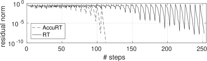
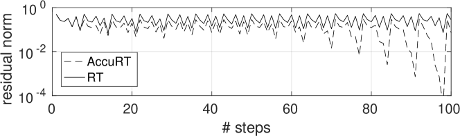
Figure 5: Convergence of the SAI Krylov method with RT (solid line) and AccuRT (dashed line) restarting for lossless Maxwell equations test, mesh $40\times 40\times 40$, restart length 7. The bottom plot is a close up of the top plot. Each zigzag corresponds to a restart.

Our experience indicates that, to have a fast convergence with SAI Krylov methods for strongly nonsymmetric matrices $A$, $\gamma$ should be taken significantly smaller than the commonly used value $t/10$ [6]. Hence we set $\gamma$ to $t/80=1/80$ for both RT and AccuRT methods, and the AccuRT restarting can eventually further decrease this value. The results are presented in Table 2 and in Figures 5 and 6. The AccuRT restarting clearly outperforms the RT restarting both in terms the costs and the attained accuracy. The accuracy loss occurs at the first restarts when the residual norm turns out to be nowhere within the required tolerance. The AccuRT then reduces $\gamma$ which not only repairs the accuracy loss but also leads to a faster solution of the shifted systems (the smaller $\gamma$, the faster unpreconditioned GMRES converges). Moreover, the reduced $\gamma$ leads then to a further efficiency gain by AccuRT. As can be seen in Figure 6, it is obtained due to larger intervals $[0,\delta]$ on which the residual appears to be smaller than the required tolerance (recall that the time interval at each restart reduces from $[0,t]$ to $[0,t-\delta]$).

Table 2: Results for the lossless Maxwell equation test problem, final time $t=1$.

Method	Tolerance,	CPU	Steps (inner
	error	time (s)	iterations)
mesh $40\times 40\times 40$, restart length 7
RT, GMRES(10)	1e-09, 2.97e-07	138.1	252 (2268)
AccuRT, GMRES(10)	1e-09, 6.60e-08	50.3	112 (798)
mesh $80\times 80\times 80$, restart length 8
RT, GMRES(10)	1e-09, 7.20e-07	1888	312 (3781)
AccuRT, GMRES(10)	1e-09, 3.92e-08	785	191 (1410)

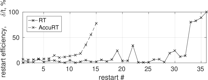
Figure 6: Restarting efficiency as a ratio of the decreased time interval length $\delta$ and total remaining time interval length $t$ for the lossless Maxwell equations test, mesh $40\times 40\times 40$, restart length 7. Efficiency $0\%$ at the first restart means that $\gamma$ is decreased by AccuRT.

4 Conclusions

The presented AccuRT (accurate residual–time) restarting seems to be a promising approach for SAI (shift-and-invert) Krylov subspace methods evaluating the matrix exponential of nonsymmetric matrices. It has all the attractive properties of the standard RT (residual–time) restarting and allows to avoid its accuracy loss while preserving efficiency of the method.

Several research directions for further studies can be indicated. First, the minimum search of the residual norm is currently carried out on a uniform set of points spread over the time interval. This could also be done on a nonuniform grid refined in the regions where the residual norm has its local minima. An adaptive procedure for building such a mesh could be designed. Furthermore, a question on how to extend this approach to symmetric matrices could be investigated. We hope to address these issues in the future.

References

- [1] M. Afanasjew, M. Eiermann, O. G. Ernst, and S. Güttel. Implementation of a restarted Krylov subspace method for the evaluation of matrix functions. Linear Algebra Appl., 429:2293–2314, 2008.
- [2] A. H. Al-Mohy and N. J. Higham. Computing the action of the matrix exponential, with an application to exponential integrators. SIAM J. Sci. Comput., 33(2):488–511, 2011. http://dx.doi.org/10.1137/100788860.
- [3] R. Barrett, M. Berry, T. F. Chan, J. Demmel, J. Donato, J. Dongarra, V. Eijkhout, R. Pozo, C. Romine, and H. A. van der Vorst. Templates for the Solution of Linear Systems: Building Blocks for Iterative Methods. SIAM, Philadelphia, PA, 1994. Available at www.netlib.org/templates/.
- [4] L. Bergamaschi and M. Vianello. Efficient computation of the exponential operator for large, sparse, symmetric matrices. Numerical linear algebra with applications, 7(1):27–45, 2000.
- [5] R.-U. Börner, O. G. Ernst, and S. Güttel. Three-dimensional transient electromagnetic modelling using rational Krylov methods. Geophysical Journal International, 202(3):2025–2043, 2015.
- [6] M. A. Botchev. Krylov subspace exponential time domain solution of Maxwell’s equations in photonic crystal modeling. J. Comput. Appl. Math., 293:24–30, 2016. http://dx.doi.org/10.1016/j.cam.2015.04.022.
- [7] M. A. Botchev, V. Grimm, and M. Hochbruck. Residual, restarting and Richardson iteration for the matrix exponential. SIAM J. Sci. Comput., 35(3):A1376–A1397, 2013. http://dx.doi.org/10.1137/110820191.
- [8] M. A. Botchev, A. M. Hanse, and R. Uppu. Exponential Krylov time integration for modeling multi-frequency optical response with monochromatic sources. Journal of Computational and Applied Mathematics, 340:474–485, 2018. https://doi.org/10.1016/j.cam.2017.12.014.
- [9] M. A. Botchev and L. A. Knizhnerman. ART: Adaptive residual-time restarting for Krylov subspace matrix exponential evaluations. Journal of Computational and Applied Mathematics, 364(112311), 2020.
- [10] E. Celledoni and I. Moret. A Krylov projection method for systems of ODEs. Appl. Numer. Math., 24(2-3):365–378, 1997.
- [11] V. Druskin, L. Knizhnerman, and M. Zaslavsky. Solution of large scale evolutionary problems using rational Krylov subspaces with optimized shifts. SIAM Journal on Scientific Computing, 31(5):3760–3780, 2009.
- [12] V. L. Druskin, A. Greenbaum, and L. A. Knizhnerman. Using nonorthogonal Lanczos vectors in the computation of matrix functions. SIAM J. Sci. Comput., 19(1):38–54, 1998.
- [13] V. L. Druskin and L. A. Knizhnerman. Two polynomial methods of calculating functions of symmetric matrices. U.S.S.R. Comput. Maths. Math. Phys., 29(6):112–121, 1989.
- [14] M. Eiermann, O. G. Ernst, and S. Güttel. Deflated restarting for matrix functions. SIAM J. Matrix Anal. Appl., 32(2):621–641, 2011.
- [15] A. Frommer and V. Simoncini. Matrix functions. In W. H. A. Schilders, H. A. van der Vorst, and J. Rommes, editors, Model Order Reduction: Theory, Research Aspects and Applications, pages 275–304. Springer, 2008.
- [16] G. H. Golub and C. F. Van Loan. Matrix Computations. The Johns Hopkins University Press, Baltimore and London, third edition, 1996.
- [17] S. Güttel. Rational Krylov Methods for Operator Functions. PhD thesis, Technischen Universität Bergakademie Freiberg, March 2010. www.guettel.com.
- [18] S. Güttel. Rational Krylov approximation of matrix functions: Numerical methods and optimal pole selection. GAMM Mitteilungen, 36(1):8–31, 2013. www.guettel.com.
- [19] S. Güttel, A. Frommer, and M. Schweitzer. Efficient and stable Arnoldi restarts for matrix functions based on quadrature. SIAM J. Matrix Anal. Appl, 35(2):661–683, 2014.
- [20] N. J. Higham. Functions of Matrices: Theory and Computation. Society for Industrial and Applied Mathematics, Philadelphia, PA, USA, 2008.
- [21] M. Hochbruck and C. Lubich. On Krylov subspace approximations to the matrix exponential operator. SIAM J. Numer. Anal., 34(5):1911–1925, Oct. 1997.
- [22] M. Hochbruck and C. Lubich. Exponential integrators for quantum-classical molecular dynamics. BIT, 39(4):620–645, 1999.
- [23] M. Hochbruck and A. Ostermann. Exponential integrators. Acta Numer., 19:209–286, 2010.
- [24] M. Hochbruck, T. Pažur, A. Schulz, E. Thawinan, and C. Wieners. Efficient time integration for discontinuous Galerkin approximations of linear wave equations. ZAMM, 95(3):237–259, 2015.
- [25] W. Hundsdorfer and J. G. Verwer. Numerical Solution of Time-Dependent Advection-Diffusion-Reaction Equations. Springer Verlag, 2003.
- [26] T. Jawecki, W. Auzinger, and O. Koch. Computable strict upper bounds for Krylov approximations to a class of matrix exponentials and -functions. arXiv preprint arXiv:1809.03369, 2018. https://arxiv.org/pdf/1809.03369.
- [27] L. A. Knizhnerman. Calculation of functions of unsymmetric matrices using Arnoldi’s method. U.S.S.R. Comput. Maths. Math. Phys., 31(1):1–9, 1991.
- [28] J. S. Kole, M. T. Figge, and H. De Raedt. Unconditionally stable algorithms to solve the time-dependent Maxwell equations. Phys. Rev. E, 64:066705, 2001.
- [29] L. A. Krukier. Implicit difference schemes and an iterative method for solving them for a certain class of systems of quasi-linear equations. Sov. Math., 23(7):43–55, 1979. Translation from Izv. Vyssh. Uchebn. Zaved., Mat. 1979, No. 7(206), 41–52 (1979).
- [30] C. B. Moler and C. F. Van Loan. Nineteen dubious ways to compute the exponential of a matrix, twenty-five years later. SIAM Rev., 45(1):3–49, 2003.
- [31] I. Moret and P. Novati. RD rational approximations of the matrix exponential. BIT, 44:595–615, 2004.
- [32] J. Niehoff. Projektionsverfahren zur Approximation von Matrixfunktionen mit Anwendungen auf die Implementierung exponentieller Integratoren. PhD thesis, Mathematisch-Naturwissenschaftlichen Fakultät der Heinrich-Heine-Universität Düsseldorf, December 2006.
- [33] B. N. Parlett. The Symmetric Eigenvalue Problem. SIAM, 1998.
- [34] Y. Saad. Iterative Methods for Sparse Linear Systems. SIAM, 2d edition, 2003. Available from http://www-users.cs.umn.edu/~saad/books.html.
- [35] R. B. Sidje. Expokit. A software package for computing matrix exponentials. ACM Trans. Math. Softw., 24(1):130–156, 1998. www.maths.uq.edu.au/expokit/.
- [36] A. Taflove and S. C. Hagness. Computational electrodynamics: the finite-difference time-domain method. Artech House Inc., Boston, MA, third edition, 2005.
- [37] H. Tal-Ezer. On restart and error estimation for Krylov approximation of . SIAM J. Sci. Comput., 29(6):2426–2441, 2007.
- [38] J. van den Eshof and M. Hochbruck. Preconditioning Lanczos approximations to the matrix exponential. SIAM J. Sci. Comput., 27(4):1438–1457, 2006.
- [39] H. A. van der Vorst. Iterative Krylov methods for large linear systems. Cambridge University Press, 2003.
- [40] J. G. Verwer and M. A. Botchev. Unconditionally stable integration of Maxwell’s equations. Linear Algebra and its Applications, 431(3–4):300–317, 2009.