Thermoelectric power of Sachdev-Ye-Kitaev islands:
Probing Bekenstein-Hawking entropy in quantum matter experiments

Abstract

The Sachdev-Ye-Kitaev (SYK) model describes electrons with random and all-to-all interactions, and realizes a many-body state without quasiparticle excitations, and a non-vanishing extensive entropy $S_{0}$ in the zero temperature limit. Its low energy theory coincides the low energy theory of the near-extremal charged black holes with Bekenstein-Hawking entropy $S_{0}$. Several mesoscopic experimental configurations realizing SYK quantum dynamics over a significant intermediate temperature scale have been proposed. We investigate quantum thermoelectric transport in such configurations, and describe the low temperature crossovers out of SYK criticality into regimes with either Fermi liquid behavior, a Coulomb blockade, or criticality associated with Schwarzian quantum gravity fluctuations. Our results show that thermopower measurements can serve as a direct probe for $S_{0}$.

I Introduction

The Sachdev-Ye-Kitaev (SYK) model Sachdev and Ye (1993); Kitaev (2015) is a strongly interacting quantum many-body system without quasiparticle excitations that is maximally chaotic, nearly conformally invariant, and exactly solvable in the limit of large number of interacting particles. It also provide a simple holographic model of charged black holes with AdS₂ horizons, and the low energy theories of black holes and the SYK model coincide both at leading Sachdev (2010, 2015) and sub-leading order Kitaev (2015); Kitaev and Suh (2019); Maldacena and Stanford (2016); Maldacena et al. (2016); Engelsöy et al. (2016); Jensen (2016); Moitra et al. (2019); Sachdev (2019).

There have been a number of interesting proposals towards realizing mesoscopic strongly-interacting correlated electron systems in the presence of disorder and narrow single-particle bandwidth Pikulin and Franz (2017); Chew et al. (2017); Chen et al. (2018); Can et al. (2019); others have advocated realization by quantum gates García-Álvarez et al. (2017). Here, we focus on the ‘quantum simulation’ point-of-view in the mesoscopic realizations. These have the added benefit of providing insight into the relevance of SYK to the naturally occurring correlated electron systems Altland et al. (2019). A particularly attractive experimental configuration can be built on the zeroth Landau level in irregular-shaped flakes of graphene Chen et al. (2018), however our study addresses a more general case of SYK islands independently of various possible physical realizations.

The existing theoretical studies of such mesoscopic ‘SYK islands’ have focused on electrical transport between the SYK island and a normal metal lead Pikulin and Franz (2017); Chew et al. (2017); Chen et al. (2018); Can et al. (2019); Gnezdilov et al. (2018); Altland et al. (2019). Here we extend these analyses to thermoelectric transport in general. We will show below that the thermopower $\Theta$ of an SYK island offers a direct probe of the entropy per particle. In particular, such measurements should be able to extract a unique feature of the SYK model, its non-vanishing extensive entropy in the low temperature ($T$) limit, $S_{0}\neq 0$. And this residual entropy is directly connected to the Bekenstein-Hawking entropy of extremal charged black holes Sachdev (2010).

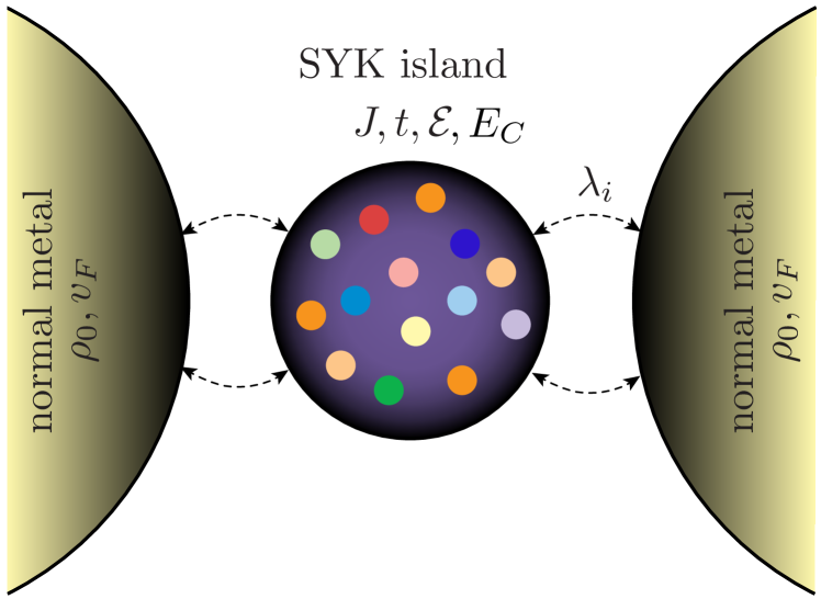
Figure 1: A sketch for an SYK island (center) characterized by a random interaction of mean-square strength $J$, a random electron hopping of mean-square strength $t$, and a dimensionless particle-hole asymmetry parameter $\mathcal{E}$. The island is coupled to normal metal leads by hopping $\lambda_{i}$, and this is characterized by an energy scale $\Gamma\propto|\lambda_{i}|^{2}\times$ (density of states in the leads). The SYK behavior requires $\Gamma,t\ll J$.

In any realistic experimental configuration, SYK criticality (and the black hole mapping) is only expected to exist in an intermediate temperature scale below the SYK random interaction scale $J$, and above a lower cutoff energy scale. Depending upon the experimental configuration, there are different possibilities for the largest lower energy scale:

1. The ‘coherence’ scale

   $$E_{\rm coh}=\frac{t^{2}}{J}\,,$$ (1)

   where $t$ is the bandwidth of the single-particle states. We always assume $t<J$, for otherwise the SYK regime does not exist at any $T$. For $T<E_{\rm coh}$, quasiparticles re-emerge, and there is a Fermi liquid regime, whose properties will be recalled in Section III.2. The crossover from SYK to Fermi liquid behavior will be described in Section III.1.

2. The charging energy $E_{C}$. For $T<E_{C}$, the Coulomb blockade appears, and its interplay with SYK criticality was investigated partly in Ref. Altland et al., 2019, but not for the case of thermopower. We will describe this crossover in Section IV.

3. The interaction energy scale $J/N$, where $N$ is the number of single particle states. The crossover at $T\sim J/N$ is associated with quantum gravity fluctuations described by the Schwarzian theory Kitaev (2015); Kitaev and Suh (2019); Maldacena and Stanford (2016); Gu et al. (2020). This crossover has been investigated numerically in Ref. Kobrin et al., 2020, but not for transport observables. We will discuss it in Section V.

Our paper will investigate the associated crossovers out of SYK criticality at these 3 energy scales, especially in the thermopower.

Fig. 1 illustrates another energy scale, $\Gamma$, associated with the coupling to the metallic leads. All our results in this paper will be in the limit $\Gamma\rightarrow 0$.

I.1 SYK criticality and thermopower

This subsection will recall some of the key properties of the SYK criticality, obtained when all the 4 energy scales just noted are vanishingly small. We also outline our main new results on the thermopower.

Of particular interest to us is how the properties of the complex SYK model (a model built on complex fermions), evolve as a function of the conserved $U(1)$ charge, the electron density $\mathcal{Q}$. The ground state of this model realizes a critical phase, over a range of values of the chemical potential $\mu$, or $\mathcal{Q}$. For a model with mean-square random interaction of strength $J$, the imaginary time electron Green’s function obeys at times $|\tau|\gg 1/J$

$$G(\tau)\sim\left\{\begin{array}[]{ccc}-\tau^{-2\Delta}&{}\hfil&\tau>0\\ e^{-2\pi\mathcal{E}}(-\tau)^{-2\Delta}&{}\hfil&\tau<0\end{array}\right.\quad,\quad T=0$$ (2)

where $\Delta=1/4$ is the scaling dimension of the electron operators. Our interest here focuses particularly on the particle-hole asymmetry $\mathcal{E}$, which can be expressed as a function of $\mathcal{Q}$ via a Luttinger-like relation Georges et al. (2001); Davison et al. (2017); Gu et al. (2020).

$$\mathcal{E} =\frac{1}{2\pi}\ln\frac{\sin(\pi\Delta+\theta)}{\sin(\pi\Delta-\theta)},$$

$$\mathcal{Q} =\frac{1}{2}-\frac{\theta}{\pi}+\left(\Delta-\frac{1}{2}\right)\frac{\sin(2\theta)}{\sin(2\pi\Delta)}\,.$$ (3)

For the specific case of the pure SYK model with infinite-range interactions, numerical studies Sachdev and Ye (1993); Georges et al. (2000, 2001); Fu and Sachdev (2016); Azeyanagi et al. (2018) show that solutions with variable $\mathcal{Q}$ and $\mathcal{E}$ exist for $0.2<\mathcal{Q}<0.8$ or $|\mathcal{E}|<0.14$ Azeyanagi et al. (2018); Patel and Sachdev (2019).

Note that the particle-hole asymmetry in (2) is significantly stronger than that in a Fermi liquid case. Even in the presence of an energy dependent density of states, the electron Green’s function of a Fermi liquid is particle-hole symmetric, with $G(\tau)\sim-{1}/{\tau}$ at large $|\tau|$, with the same amplitude for both signs of $\tau$. So formally, $\mathcal{E}=0$ for a Fermi liquid.

The strong particle-hole asymmetry of the SYK model is intimately connected to its extensive entropy as $T\rightarrow 0$ via the relation Georges et al. (2001); Davison et al. (2017); Gu et al. (2020)

$$\frac{d\mathcal{S}}{d\mathcal{Q}}=2\pi\mathcal{E},$$ (4)

where $N$ is the number of sites in the SYK model, and $\mathcal{S}\equiv S_{0}/N$ is entropy density in the limit where $N\rightarrow\infty$ first, followed later by $T\rightarrow 0$. (Eq. (4) also shows that $\mathcal{E}=0$ in a Fermi liquid, because $\mathcal{S}$ vanishes as $T\rightarrow 0$ in a Fermi liquid.) The relationship (4) was obtained by Georges et al. Georges et al. (2001), building upon large $N$ studies of the multichannel Kondo problem Parcollet et al. (1998). Independently, this relationship appeared as a general property of black holes with AdS₂ horizons Sen (2005, 2008), where $\mathcal{E}$ is identified with the electric field on the horizon Faulkner et al. (2011).

We now turn to the thermopower, $\Theta$, and its connection to the entropy. In Fermi liquids, the thermopower is usually computed by the ‘Mott formula’

$$\Theta=\frac{\pi^{2}}{3}\frac{k_{B}^{2}T}{e}\frac{\partial\ln\sigma}{\partial\epsilon_{F}},$$ (5)

where $\sigma$ is conductivity at Fermi energy $\epsilon_{F}$ (we set $k_{B}=1$ elsewhere). Note that the thermopower vanishes as $T\rightarrow 0$, and is proportional to particle-hole asymmetries which lead to a Fermi energy dependence in the conductivity. If we assume that such dependence is entirely due to the density of states (and not due to the scattering time), then (5) can be written as

$$\Theta=\frac{1}{e}\frac{d\mathcal{S}}{d\mathcal{Q}},$$ (6)

an expression dubbed as the ‘Kelvin formula’ in Ref. Peterson and Shastry, 2010.

As the entropy vanishes linearly with $T$ in a Fermi liquid, (6) implies that the thermopower also vanishes linearly with $T$. The Kelvin formula was originally proposed as an approximate empirical formula useful in certain strongly correlated systems Peterson and Shastry (2010); Mravlje and Georges (2016).

Turning to thermopower in systems without quasipasiparticles, Davison et al Davison et al. (2017) showed that the Kelvin formula was exact for transport in lattices of coupled SYK islands. Given the non-vanishing of $\mathcal{S}$ as $T\rightarrow 0$, this implies that $\Theta$ also remains non-zero as $T\rightarrow 0$, in striking contrast from a Fermi liquid. It was also found Davison et al. (2017) that the Kelvin formula was an exact general feature of charged black holes with AdS₂ horizons. We are interested here in transport between a single SYK island and normal metal leads, a general idea is sketched in Fig. 1 (in contrast to transport between 2 SYK islands in the lattice models Gu et al. (2017); Davison et al. (2017); Song et al. (2017); Zhang (2017); Chowdhury et al. (2018); Patel et al. (2018)). One of our new results is that in the single-channel lead configuration, and under conditions in which the transport is dominated by SYK correlations (specified more carefully in the body of the paper), we have the thermopower

$$\Theta=\frac{2}{3e}\,2\pi\mathcal{E}.$$ (7)

So as in other systems, the thermopower is intimately connected to the $\mathcal{Q}$ dependence of the entropy, via (4). One of our main observations is that the relations (2), (4), and (7) link together the surprising features of the SYK model: (i) the strong particle-hole asymmetry in the low energy limit, (ii) the non-vanishing extensive entropy as $T\rightarrow 0$, and (iii) the non-vanishing thermoelectric power as $T\rightarrow 0$.

The outline of the remainder of the paper is as follows. We will setup the basic formalism for the transport across SYK islands in Section II. To set the stage, Section III.2 will investigate the familiar disordered Fermi liquid regime, when $E_{\rm coh}$ is the largest of the low energy cutoffs, and $T<E_{\rm coh}$. Then Sections III.1, IV, and V will discuss the low $T$ crossover out of SYK criticality controlled by the 3 energy scales noted earlier in this introduction. We will discuss possible values of experimental parameters, and these energy scales in Section VI.

II Setup

We will model the SYK island by a Hamiltonian, $H_{\text{I}}$ with random interactions and hopping, and a bare charging energy $E_{C}^{0}$:

$$H_{\text{I}}=\frac{1}{(2N)^{3/2}}\sum_{ij;kl=1}^{N}J_{ij;kl}c^{{\dagger}}_{i}c^{{\dagger}}_{j}c_{k}c_{l}$$

$$+\frac{1}{N^{1/2}}\sum_{ij=1}^{N}t_{ij}c^{{\dagger}}_{i}c_{j}-\mu\sum_{i}c^{{\dagger}}_{i}c_{i}+\frac{E_{C}^{0}}{2}\left(\sum_{i}c^{{\dagger}}_{i}c_{i}\right)^{2}\,.$$

Here $J_{ij;kl}$ is random interaction with zero mean and root-mean-square magnitude $J$ ($\langle J_{ij;kl}\rangle=0$, $\langle|J_{ij;kl}|^{2}\rangle=J^{2}$), and $t_{ij}$ is random hopping with zero mean and root-mean-square magnitude $t$ ($\langle t_{ij}\rangle=0$, $\langle|t_{ij}|^{2}\rangle=t^{2}$). The bare charging energy $E_{C}^{0}$ is renormalized to $E_{C}$ by the $J_{ij;kl}$ interactions, as was computed in Ref. Gu et al., 2020; we will use the renormalized $E_{C}$ in all our results.

The large $N$ retarded electron Green’s function, $\mathcal{G}(\omega)$ can be computed numerically at $E_{C}=0$ for all $\omega$, $T$, $\mu$, $J$, and $t$ by solving a set of integro-differential equations. The solutions of these equations where described elsewhere in the literature Parcollet and Georges (1999); Song et al. (2017) for $\mathcal{E}=0$. We have extended these numerics to non-zero $\mathcal{E}(\mathcal{Q})$, with

$$\mathcal{Q}=\frac{1}{N}\sum_{i}\langle c^{{\dagger}}_{i}c_{i}\rangle\,,$$ (9)

and will describe the implications for thermoelectric transport in Section III. We will also describe the extension to non-zero $E_{C}$ (at $t=0$) in Section IV, and the Schwarzian fluctuations at non-zero $J/N$ in Section V.

A crucial feature of this solution for $t\ll J$ (which we assume throughout) is the emergence of a low energy scale $E_{\rm coh}$ which was defined in (1) as the first of low energy cutoffs for SYK behavior. When $E_{\rm coh}$ is the largest of the low energy cutoffs, then for $T<E_{\rm coh}$ (but $T$ larger than the other of the low energy cutoffs), we recover the physics of a disordered Fermi liquid, albeit with strong renormalization from the interactions.

Let us now couple the island to the leads (Fig. 1). Here we follow the approach of Gnezdilov et al. Gnezdilov et al. (2018), and model the leads by

$$\mathcal{H}=H_{\text{I}}+\sum_{\mathbf{q}}\varepsilon_{\mathbf{q}}\,a^{{\dagger}}_{\mathbf{q}}a_{\mathbf{q}}+\sum_{i,\mathbf{q}}\lambda_{i}c^{{\dagger}}_{i}a_{\mathbf{q}}+\lambda^{*}_{i}a^{{\dagger}}_{\mathbf{q}}c_{i}.$$ (10)

The new terms represent dispersive electrons ($a^{{\dagger}}_{\mathbf{p}}$, $a_{\mathbf{p}}$) in the single-channel contact with a dispersion $\varepsilon_{\mathbf{q}}$ near the Fermi surface. The SYK quantum dot fermions $c^{{\dagger}}_{i}$ and the lead fermions with $a_{\mathbf{p}}$ are coupled by the random hopping $\lambda_{i}$. The coupling to the leads will be characterized by the energy scale

$$\Gamma=\pi\rho_{\rm lead}\sum_{i}|\lambda_{i}|^{2},$$ (11)

where $\rho_{\rm lead}$ is the density of states in the lead. In the limit $\Gamma\rightarrow 0$, the non-linear electrical transport of $\mathcal{H}$ is described by the differential conductance Gnezdilov et al. (2018); Costi and Zlatić (2010)

$$\frac{dI}{dV}=\frac{4\Gamma e^{2}}{h}\int_{-\infty}^{\infty}d\omega f^{\prime}(\omega-eV)\mbox{Im}\mathcal{G}(\omega)$$ (12)

where $\mathcal{G}$ is the retarded Green’s function of $H_{I}$ alone, $f(\omega)=1/(e^{\omega/T}+1)$ is the Fermi function, and a factor of 2 for electron spin has been included.

For linear thermoelectric transport, we use expressions derived by Costi and Zlatić Costi and Zlatić (2010). We define

$$\mathcal{L}_{ij}=\frac{2\Gamma}{\pi\hbar}\int\limits_{-\infty}^{+\infty}d\omega\,\omega^{i+j-2}f^{\prime}(\omega)\text{Im}\mathcal{G}(\omega)\,.$$ (13)

Then we have for the electric conductance $\sigma$, thermal conductance $\kappa$, and the thermopower $\Theta$ (see also Ref. Mahan, 1981; Xu et al., 2011)

$$\sigma = e^{2}\,\mathcal{L}_{11},$$

$$\kappa = \beta\left(\mathcal{L}_{22}-\frac{\mathcal{L}_{12}^{2}}{\mathcal{L}_{11}}\right),$$

$$\Theta = \frac{\beta}{e}\frac{\mathcal{L}_{12}}{\mathcal{L}_{11}},$$ (14)

where $\beta=1/T$. The following sections will evaluate these expressions in different regimes depending upon the relative values of the small energy scales $T$, $E_{\rm coh}$, and $E_{C}$.

III Crossover from SYK to Fermi Liquid

We begin with the case in which $E_{\rm coh}$ in (1) is the largest of low energy cutoff scales i.e. $E_{\rm coh},T\gg J/N,E_{C}$. Then there is a crossover from SYK criticality for $E_{\rm coh}\ll T\ll J$ to a Fermi liquid regime for $E_{C}\ll T\ll E_{\rm coh}$.

A full description of the crossover requires numerical results for $\mathcal{G}(\omega)$, which generalize the earlier computations Parcollet and Georges (1999); Song et al. (2017) to non-zero $\mathcal{E}$. Our numerical results for crossover bewteen these two regimes at fixed filling $\mathcal{Q}$ are presented in Fig. 2.

More complete analytic results are possible for the limiting SYK regime for $E_{\rm coh}\ll T\ll J$, and for the Fermi liquid regime for $T\ll E_{\rm coh}$, and we will present them in the following subsections.

III.1 Pure SYK regime

We consider the main regime of interest to us, when $T$ is larger than all the low energy cutoffs mentioned in Section I, but we have $T\ll J$.

To leading order, we may set $E_{\rm coh}=0$. Analytic expressions for the Green’s function are possible for $t/J=0$ and $T\ll J$. Then we can use the conformal form of the (retarded) SYK Green’s function

$$\mathcal{G}(\omega)= -ie^{-i\theta}\left(\frac{\pi}{\cos 2\theta}\right)^{1/4}\left(\frac{\beta}{2\pi J}\right)^{1/2}$$

$$\times\frac{\bm{\Gamma}({\frac{1}{4}-\frac{i}{2\pi}\beta\omega}+i\mathcal{E})}{\bm{\Gamma}({\frac{3}{4}-\frac{i}{2\pi}\beta\omega}+i\mathcal{E})},$$ (15)

where $\bm{\Gamma}(x)$ is the Gamma function.

We find that the SYK state has a finite, temperature-independent thermopower, a consequence of finite Bekenstein-Hawking entropy $S_{0}$ associated with the SYK state. In the case of single-island pure SYK flake we find the thermopower $\Theta$ is directly connected to particle-hole asymmetry $\mathcal{E}$:

$$\Theta=\frac{\beta}{e}\frac{\int_{-\infty}^{+\infty}d\omega\,\omega f^{\prime}(\omega)\,\mbox{Im}\mathcal{G}(\omega)}{\int_{-\infty}^{+\infty}d\omega f^{\prime}(\omega)\,\mbox{Im}\mathcal{G}(\omega)}=\frac{4\pi}{3e}\mathcal{E}.$$ (16)

This $T$-independent thermopower holds for $T>E_{\rm coh}\sim t^{2}/J$, and vanishes linearly with $T$ in the Fermi liquid regime $T<E_{\rm coh}$ (we are assuming here that the other cutoff energy scales discussed in Section I are even smaller than $E_{\rm coh}$

Figure 2: Crossovers in transport from the SYK regime at $T>E_{\rm coh}$, to Fermi liquid behavior at $T<E_{\rm coh}$. There is no divergence in the conductances as $T\rightarrow 0$, and they saturate at values related to those in (24), with an energy scale of order $E_{\rm coh}$ replacing $t,\mu$. It is assumed here that $T,E_{\rm coh}\gg E_{C},J/N$. We use $J=10$, $t=0.1$, and $\mathcal{Q}=1/3$.

It is useful to compare (16) with the result obtained for the case of thermoelectric transport between SYK islands, in contrast to the transport with normal metal leads, as in Fig. 1. Then the corresponding expression for the thermopower was obtained by Patel et al. Patel et al. (2018)

$$\Theta=\frac{\beta}{e},\frac{\int_{-\infty}^{+\infty}d\omega\,\omega f^{\prime}(\omega)\,[\mbox{Im}\mathcal{G}(\omega)]^{2}}{\int_{-\infty}^{+\infty}d\omega f^{\prime}(\omega)\,[\mbox{Im}\mathcal{G}(\omega)]^{2}}=\frac{2\pi}{e}\mathcal{E}.$$ (17)

Note that we now have 2 powers of the Green’s function in the numerator and denominator because both the initial and final locations of the electron are on SYK islands. Moreover, we find that the Kelvin relation (6) is then precisely satisfied.

The remaining transport properties in the SYK regime can be obtained by inserting (15) into the expressions in Section II. We obtain for $T\ll J$, and $T\gg E_{\rm coh},J/N,E_{C}$:

$$e\Theta = \frac{4\pi}{3}{\color[rgb]{0,0,1}\mathcal{E}},$$

$$\frac{\hbar\sigma}{\Gamma e^{2}} = \left[0.72+\mathcal{O}(\mathcal{E}^{2})\right]\frac{1}{\sqrt{JT}}$$

$$\frac{\hbar\kappa}{\Gamma T} = \left[1.42+\mathcal{O}(\mathcal{E}^{2})\right]\frac{1}{\sqrt{JT}}$$ (18)

(the exact value of conductance prefactor is $2\sqrt{2}\pi^{-1/4}\Gamma(3/4)/\Gamma(1/4)=0.72$). The Lorenz ratio linking electrical and thermal conductance is

$$\frac{e^{2}\kappa}{\sigma T}=\frac{\pi^{2}}{5}+\frac{1}{5}\left(\frac{4\pi}{3}\mathcal{E}\right)^{2},$$ (19)

and is $T$-independent, but its value is distinct from the Lorenz number $=\pi^{2}/3\approx 3.29$ in a Fermi liquid.

Recently, themoelectric cooling and power generation in nanodevices, characterized by computed thermoelectric figure of merit, has attracted significant attention Roura-Bas et al. (2018); Sheng and Fu (2019); Fu (2019). We calculate this quantity for a SYK island. The maximum efficiency of electricity generation by a thermoelectric device is typically described in terms of its figure of merit $Z$:

$$Z=\frac{\mathcal{L}_{12}^{2}}{\det\mathcal{L}_{ij}}=\frac{\Theta^{2}\sigma T}{\kappa}\,.$$ (20)

For SYK criticality, thethermoelectric figure of merit is

$$Z=\frac{5(e\Theta)^{2}}{\pi^{2}+(e\Theta)^{2}}\,.$$ (21)

This can be larger than in a Fermi liquid which has $Z\sim(T/E_{F})^{2}$, where $E_{F}$ is the Fermi energy.

III.2 Fermi liquid regime

Next, we present the familiar results in the Fermi liquid regime $T\ll E_{\rm coh}$, but $T\gg E_{C}$. The random SYK interactions are formally irrelevant, and can be accounted for by a renormalization in the value of $t$ to $E_{\rm coh}$ Parcollet and Georges (1999); Song et al. (2017). We just present the results without this renormalization here, but it should be kept in mind that for the results in this section $t$ should be replaced by an energy of order $E_{\rm coh}$ when $t\ll J$.

The Green’s function can be computed exactly in the absence of interactions by solving a quadratic equation Parcollet and Georges (1999)

$$\mathcal{G}(\omega)=\frac{1}{2t^{2}}\left(\omega+\mu-\sqrt{(\omega+\mu)^{2}-4t^{2}}\right)\,,$$ (22)

which yields the well-known semi-circular density of states of a random matrix. We denote

$$\rho = -\frac{1}{\pi}\mbox{Im}\mathcal{G}(0)$$

$$\rho^{\prime} = -\frac{1}{\pi}\left.\frac{d}{d\omega}\mbox{Im}\mathcal{G}(\omega)\right|_{\omega=0}\,,$$ (23)

as the density of states, and its derivative, at the Fermi level. Then the thermoelectric responses are

$$e\Theta = \frac{\pi^{2}T}{3}\frac{\rho^{\prime}}{\rho}$$

$$\frac{\hbar\sigma}{\Gamma e^{2}} = 2\rho$$

$$\frac{\hbar\kappa}{\Gamma T} = \frac{2\pi^{2}}{3}\rho\,.$$ (24)

As we can see, the thermopower $\Theta$ vanishes as $T\to 0$, which is a general phenomenon for interacting matter with quasiparticles. Both the Mott Law and Wiedemann-Franz Law hold, and the Lorentz number is $L=e^{2}\kappa/(\sigma T)={\pi^{2}}/{3}$, as well as the Mott number is $M=\Theta/(T\rho^{\prime}/(e\rho))={\pi^{2}}/{3}$.

IV Charging energy

We now turn to the case where the charging energy $E_{C}$ is the largest of the low energy cutoffs. We will consider the crossover around $T\sim E_{C}$, with $T<J$, as always. But in this section we assume $E_{C}\gg E_{\rm coh},J/N$.

Here we have consider the consequences of fluctuations in the total charge, $Q=N\mathcal{Q}$, of the SYK ideal. A complete theory for such fluctuations was presented recently in Ref. Gu et al., 2020, and we recall essential aspects for our purposes.

We need the corrections to the SYK Green’s function from the charge fluctuations. This correction will arise from the fluctuations of a conjugate phase field $\lambda(\tau)$, and a time reparameterization field $\varphi(\tau)$. From Eqs (2.47) and (2.48) of Ref. Gu et al., 2020, the Green’s function of the complex SYK model is given by

$$\mathcal{G}(\tau_{1}-\tau_{2})=-b^{\Delta}\biggl{\langle}\varphi^{\prime}(\tau_{1})^{\Delta}\varphi^{\prime}(\tau_{2})^{\Delta}$$

$$~{}~{}~{}~{}~{}~{}~{}~{}~{}~{}~{}~{}~{}~{}~{}\times\left(2\sin\frac{\varphi(\tau_{1})-\varphi(\tau_{2})}{2}\right)^{-2\Delta}$$

$$\times\exp\Bigl{[}i\lambda(\tau_{1})-i\lambda(\tau_{2})+\mathcal{E}\left(\pi-\varphi(\tau_{1})+\varphi(\tau_{2})\right)\Bigr{]}\biggr{\rangle}_{I_{{\rm eff}}[\varphi,\lambda]}$$

where the imaginary action for the fields $\varphi(\tau)$ and $\lambda(\tau)$ is given by

$$I_{{\rm eff}}[\varphi,\lambda] = -S_{0}(Q)+\frac{1}{2E_{C}}\int_{0}^{\beta}d\tau\bigl{(}\lambda^{\prime}(\tau)+i\mathcal{E}\varphi^{\prime}(\tau)\bigr{)}^{2}$$ (26)

$$- C_{\text{Sch}}\int_{0}^{\beta}d\tau\,\operatorname{Sch}\left(\tan\frac{\varphi(\tau)}{2},\,\tau\right)\,.$$

Here $\Delta=1/4$ is the scaling dimension of the electron operator, the prefactor $b$ is

$$b=\frac{(1-2\Delta)\sin(2\pi\Delta)}{2\pi J^{2}(\cosh(2\pi\mathcal{E})+\cos(2\pi\Delta))}\,,$$ (27)

$S_{0}(Q)$ is the zero temperature entropy at the equilibrium total charge $Q$, the field $\varphi(\tau)$ is a monotonic time reparameterization obeying

$$\varphi(\tau+\beta)=\varphi(\tau)+2\pi\,,$$ (28)

and $\lambda(\tau)$ is a phase field obeying

$$\lambda(\tau+\beta)=\lambda(\tau)+2\pi n\,,$$ (29)

with integer winding number $n$ conjugate to the total charge $Q$. The notation $\operatorname{Sch}(f(x),x)$ stands for the Schwarzian derivative

$$\operatorname{Sch}(f(x),x):=\frac{f^{\prime\prime\prime}}{f^{\prime}}-\frac{3}{2}\left(\frac{f^{\prime\prime}}{f^{\prime}}\right)^{2}\,.$$ (30)

In (26), we have replaced the coupling $NK\sim N/J$ in Ref. Gu et al., 2020 by the inverse of the charging energy, $1/E_{C}$, to correspond to the notation of Ref. Altland et al., 2019, and the co-efficient of the Schwarzian, $N\gamma/(4\pi^{2})\sim N/J$, by $C_{\text{Sch}}$ to correspond to the notation of Ref. Kobrin et al., 2020.

In the leading large $N$ limit, we can replace $\varphi(\tau)$ and $\lambda(\tau)$ in (IV) by their saddle-point values $\varphi(\tau)=2\pi\tau/\beta$ and $\lambda(\tau)=0$. This yields a $\mathcal{G}(\tau)$ whose Fourier transform is (15).

We now turn to fluctuations. In the present section, with $E_{C}\gg J/N$, the fluctuations of $\lambda(\tau)$ are more important than those $\varphi(\tau)$. As the action for $\lambda(\tau)$ is Gaussian, the path integral over $\lambda$ is relatively easy to evaluate. First we consider the partition function

$$\frac{\mathcal{Z}_{\lambda}}{e^{S_{0}(Q)}}=\int\frac{\mathcal{D}\lambda}{\operatorname{U}(1)}\exp\left(-\frac{1}{2E_{C}}\int_{0}^{\beta}d\tau\bigl{(}\lambda^{\prime}(\tau)+i\mathcal{E}\varphi^{\prime}(\tau)\bigr{)}^{2}\right)\,,$$

where we have divided the integral by the volume of $\operatorname{U}(1)$ because we should view $\operatorname{U}(1)$ as a gauge symmetry. The prefactor $e^{S_{0}(Q)}$ reflects the multiplicity of the states. We will see that this partition function and the correlator needed for (IV) are independent of $\varphi(\tau)$. Related partition functions have also been evaluated recently in Ref. Liu and Zhou, 2019. We now change variables to $\tilde{\lambda}(\tau)$, where

$$\lambda(\tau)=\tilde{\lambda}(\tau)+2\pi n\frac{\tau}{\beta}+i\mathcal{E}\left(\frac{2\pi}{\beta}\tau-\varphi(\tau)\right)\,;$$ (31)

from (28) and (29) we see that $\tilde{\lambda}(\tau)$ is periodic

$$\tilde{\lambda}(\tau+\beta)=\tilde{\lambda}(\tau)\,.$$ (32)

Then we can write the path integral over $\tilde{\lambda}$ as

$$\mathcal{Z}_{\lambda} = e^{S_{0}(Q)}\left(\,\sum_{n=-\infty}^{\infty}\exp\left[-\frac{2\pi^{2}}{\beta E_{C}}(n+i\mathcal{E})^{2}\right]\right)$$ (33)

$$\times \int\frac{\mathcal{D}\tilde{\lambda}}{\operatorname{U}(1)}\exp\left[-\frac{1}{2E_{C}}\int_{0}^{\beta}d\tau\left(\tilde{\lambda}^{\prime}(\tau)\right)^{2}\right]\,.$$

The second term is just the imaginary time amplitude for a ‘free particle’ of mass $1/E_{C}$, moving on an infinite line, to return to its starting point in a time $\beta$ Sachdev (2011). In this manner, we obtain

$$\mathcal{Z}_{\lambda} = \sqrt{\frac{2\pi}{\beta E_{C}}}e^{S_{0}(Q)}\,\sum_{n=-\infty}^{\infty}\exp\left[-\frac{2\pi^{2}}{\beta E_{C}}(n+i\mathcal{E})^{2}\right]\,.$$ (34)

This expression is convergent for all values of $\beta E_{C}$, but rapidly so when $\beta E_{C}\ll 1$, when the leading contribution is just the $n=0$ term. Conversely, when $\beta E_{C}\gg 1$, it is easier to use the equivalent expression obtained from the Poisson summation formula

$$\mathcal{Z}_{\lambda} = e^{S_{0}(Q)}\,\sum_{p=-\infty}^{\infty}\exp\left[-\frac{\beta E_{C}p^{2}}{2}+2\pi\mathcal{E}p\right]$$ (35)

$$= \sum_{p=-\infty}^{\infty}e^{S_{0}(Q+p)}\exp\left[-\frac{\beta E_{C}p^{2}}{2}\right]\,,$$

where we have used (4). The expression (35) has a simple interpretation: it is the sum over states with total charge $Q+p$, with near-degeneracy $e^{S_{0}(Q+p)}$, and energy $(1/2)E_{C}p^{2}$. For $\beta E_{C}\gg 1$, the $p=0$ term dominates.

Next, we consider the Green’s function

$$\mathcal{G}_{\lambda}(\tau_{1}-\tau_{2})=$$ (36)

$$~{}\biggl{\langle}\exp\Bigl{[}i\lambda(\tau_{1})-i\lambda(\tau_{2})+\mathcal{E}\left(\pi-\varphi(\tau_{1})+\varphi(\tau_{2})\right)\Bigr{]}\biggr{\rangle}_{\mathcal{Z}_{\lambda}}\,.$$

Evaluating this with the parameterization (31), in a manner similar to $\mathcal{Z}_{\lambda}$, we obtain

$$\mathcal{G}_{\lambda}(\tau) = \exp\left[\mathcal{E}\left(\pi-\frac{2\pi}{\beta}\tau\right)\right]\frac{e^{S_{0}(Q)}}{\mathcal{Z}_{\lambda}}\sqrt{\frac{2\pi}{\beta E_{C}}}$$

$$~{}~{}~{}\times\sum_{n=-\infty}^{\infty}\exp\Biggl{[}i\frac{2\pi n}{\beta}\tau$$

$$~{}~{}~{}~{}-\frac{2\pi^{2}}{\beta E_{C}}(n+i\mathcal{E})^{2}-\frac{E_{C}}{\beta}\sum_{\omega_{m}\neq 0}\frac{1-e^{i\omega_{m}\tau}}{\omega_{m}^{2}}\Biggr{]}\,,$$

where $\omega_{m}$ is a bosonic Matsubara frequency. The summation over $\omega_{m}$ can be evaluated exactly Kamenev and Gefen (1996), and we obtain (assuming henceforth that $|\tau|\leq\beta$)

$$\mathcal{G}_{\lambda}(\tau)=\exp\left[\mathcal{E}\left(\pi-\frac{2\pi}{\beta}\tau\right)-\frac{E_{C}}{2}\left(|\tau|-\frac{\tau^{2}}{\beta}\right)\right]$$ (38)

$$\times\frac{e^{S_{0}(Q)}}{\mathcal{Z}_{\lambda}}\sqrt{\frac{2\pi}{\beta E_{C}}}\sum_{n=-\infty}^{\infty}\exp\left[i\frac{2\pi n}{\beta}\tau-\frac{2\pi^{2}}{\beta E_{C}}(n+i\mathcal{E})^{2}\right]\,.$$

This expression is rapidly convergent when $\beta E_{C}\ll 1$, and the leading answer is the $n=0$ term. For $\beta E_{C}\gg 1$, it is easier to use the equivalent expression obtained from the Poisson summation formula

$$\mathcal{G}_{\lambda}(\tau)=\frac{e^{S_{0}(Q)}}{\mathcal{Z}_{\lambda}}\exp\left[\pi\mathcal{E}-\frac{E_{C}}{2}|\tau|\right]$$ (39)

$$\times\sum_{p=-\infty}^{\infty}\exp\left[-\frac{\beta E_{C}p^{2}}{2}+2\pi p\left(\mathcal{E}-\frac{E_{C}\tau}{2\pi}\right)\right]\,.$$

The expression (39) agrees with Eq. (11) in the supplement of Ref. Altland et al., 2019.

Figure 3: Crossovers in transport from the SYK regime at $T>E_{C}$, to Coulomb blockade behavior at $T<E_{C}$. It is assumed here that $T,E_{C}\gg E_{\rm coh},J/N$. We use $J=100$ and $\mathcal{E}=0.05$. The values of $E_{C}$ are $E_{C}=0$ (red), $E_{C}=0.2$ (green), and $E_{C}=0.4$ (blue).

Returning to the full Green’s function in (IV), noting that $\mathcal{G}_{\lambda}(\tau)$ is independent of $\varphi(\tau)$, we can write

$$\mathcal{G}(\tau)=-b^{\Delta}\,\mathcal{G}_{\lambda}(\tau)\,\mathcal{G}_{\rm Sch}(\tau)$$ (40)

where $\mathcal{G}_{\lambda}(\tau)$ is specified either by (38) or (39), and $\mathcal{G}_{\rm Sch}$ is to be obtained from the Schwarzian path integral over $\varphi(\tau)$ which reduces to that evaluated earlier for the Majorana SYK model Bagrets et al. (2016); Lam et al. (2018); Yang (2019); Kobrin et al. (2020). The expression (40) is actually valid for arbitrary ratios between the energy scales $T$, $J/N$ and $E_{C}$. But for the case $T,E_{C}\gg J/N$ of interest in the present section, we can approximate the path integral over $\varphi(\tau)$ by its saddle point $\varphi(\tau)=2\pi\tau/\beta$, whence

$$\mathcal{G}_{\rm Sch}(\tau)\approx\left(\frac{\beta}{\pi}\sin\frac{\pi\tau}{\beta}\right)^{-2\Delta}\,.$$ (41)

We now take the Fourier transform of (40, 41), and analytically continue to obtain $G(\omega)$ at real frequencies; see the Appendix of Ref. Kamenev and Gefen, 1996 for a similar computation with $n=0$ term for $\mathcal{G}_{\lambda}$ in (38) at $\mathcal{E}=0$. This computation is described in Appendix A. Inserting the Green’s function so obtained, we can compute the transport properties at non-zero $E_{C}$ from the expressions in Section II: the numerical results are presented in Fig. 3.

For $T\gg E_{C}$, the results are described in Section III.1. For $E_{\rm coh},J/N\ll T\ll E_{C}$ we obtain the limiting forms

$$e\Theta\sim\mathcal{E}\frac{E_{C}}{T}$$

$$\frac{\hbar\sigma}{\Gamma e^{2}},~{}\frac{\hbar\kappa}{\Gamma T}\sim e^{-E_{C}/T}$$

$$\frac{e^{2}\kappa}{\sigma T}\sim(0.13+\mathcal{O}(\mathcal{E}^{2}))\frac{E_{C}^{2}}{T^{2}}.$$ (42)

Transport is exponentially suppressed by the charging energy in this Coulomb blockade regime. Nevertheless $\Theta\sim 1/T$ from the structure of the exponential factors. Terms higher order in the coupling to the leads, $\Gamma$, can become important in this Coulomb blockade regime Altland et al. (2019), as we will discuss briefly in Section VII.1.

V Schwarzian corrections

This section considers the case where the lower energy cutoff to SYK criticality is provided by $J/N$, the third case in Section I. In this case, the crossover at the scale $J/N$ is described by the Schwarzian quantum gravity theory. The other lower-cutoffs in Section I are presumed to be at lower energy i.e. we assume in this section that $J/N\gg E_{C},E_{\rm coh}$.

The expression (40) can also be used in the present section. Now because we assume $T,J/N\gg E_{C}$ in the present section, we can evaluate the $\lambda$ integral at the saddle point level, while the Schwarzian integral over $\varphi$ has to be exactly evaluated (note that this the complement of the method in Section IV). So we can use

$$\mathcal{G}_{\lambda}(\tau)\approx\exp\left[\mathcal{E}\left(\pi-\frac{2\pi}{\beta}\tau\right)\right]$$ (43)

which is the $n=0$ term in (38) for $\beta E_{c}\ll 1$. For $\mathcal{G}_{\rm Sch}(\tau)$, we use the expression presented in Eq. (20) of the supplement on Ref. Kobrin et al., 2020. We compute $\mathcal{G}(\omega)$ with this simplification in Appendix A. We also further compute $\mathcal{G}(\omega)$ without either of the simplifications of (41, 43) in that Appendix.

Figure 4: Crossovers in transport from the SYK regime at $T>J/N$, to Schwarizan dominated behavior at $T<J/N$. It is assumed here that $T,J/N\gg E_{\rm coh},E_{C}$. We use $J=1$ and $\mathcal{E}=0.05$. The values of $N$ are $N=\infty$ (red), $N=1000$ (green), and $N=100$ (blue).

From the $\mathcal{G}(\omega)$ so obtained, we can compute the transport properties as in Section II, leading to the numerical results presented in Fig. 4. For $T\gg J/N$, the results are described in Section III.1. For $E_{\rm coh},E_{C}\ll T\ll J/N$ we obtain the limiting forms

$$e\Theta \sim 3.1\mathcal{E}$$

$$\frac{\hbar\sigma}{\Gamma e^{2}} \sim [1.3+\mathcal{O}(\mathcal{E}^{2})]\frac{NT^{1/2}}{J^{3/2}}$$

$$\frac{\hbar\kappa}{\Gamma T} \sim [4.5+\mathcal{O}(\mathcal{E}^{2})]\frac{NT^{1/2}}{J^{3/2}}\,.$$ (44)

In this regime with $T\ll J/N$ there is a Schwarzian criticality with a fermion scaling dimension $\Delta=3/4$ Bagrets et al. (2016), and we understand the power-laws in (44) from this value.

VI Experimental parameters

We now present some estimates of parameters for the proposed realization of SYK phases in an irregular-shaped graphene flake Chen et al. (2018). Their proposal depends on the physics of Dirac electrons in strong magnetic fields. The magnetic fields should be sufficiently strong to ensure the well-defined Landau levels in a sub-micrometer graphene flake. One can work with $B\approx 10$ T in the current state of quantum transport experiments. The typical length scale set by external magnetic fields is $l_{B}=\sqrt{h/eB}$, which for $B=$10 T gives magnetic length scale $l_{B}\approx 8$ nm. We propose a graphene flake of size $L\simeq 80$ nm should allow the wavefunctions to be sensitive to the disorder originating from the edges. For such length scales, the number of states in the lowest Landau level is hundreds, $N\approx\Phi/\Phi_{0}\sim 10^{2}$. This sets the number of states for the SYK electrons $N$.

We have two initial energy scales: the strength of the SYK interactions in Ref. Chen et al., 2018 is estimated as $J\approx 25$ meV, but this is likely to decrease with the effective system size $L/l_{B}$ ($J$ vanishes for infinite-size monolayer); we take here $J\approx 10$ meV as a reasonable estimate for our $L\simeq 80$ nm flake. The finite bandwidth of the lowest Landau level (LLL) is set by bulk disorder and is estimated to be $t\approx 1$ meV in realistic samples.

These estimates yield a rather low energy for the coherence scale $E_{\rm coh}\approx 1$ K for the crossover in Section III. The crossover for the Schwarzian corrections in Section V is similar $J/N\approx 1$ K. Finally, the charging energy $E_{C}$, relevant for Section IV can be controlled by tuning the capacitance of the system independently from other effective parameters (flake size, dielectric constant, separation to the gate, and etc.). This can be achieved, for example, by putting the back gate in the proximity of the dots, which increases capacitance $C$ of the quantum dot in the controllable way. Depending on the thickness of the dielectric layer, the charging energy of the quantum dot $C$ can be tuned between 0.5 to 50 K.

VII Conclusions

The SYK model realizes a many-body state of quantum matter without quasiparticle excitaions. Its unusual properties include a non-vanishing entropy density in the zero temperature limit, and a maximal quantum Lyapunov exponent. Its low energy theory is identical to those of charged quantum black holes which also share these properties.

One of the main points of our paper is that the large low $T$ entropy density has a direct experimental signature in the thermopower. We examined in detail the experimental configuration shown in Fig. 1: with a SYK island, realized e.g. in a graphene flake as proposed in Ref. Chen et al., 2018, coupled to metallic leads. We computed the characteristic signature of SYK criticality in the electrical conductance, the thermal conductance, and the thermopower, and the main results are in (18).

Every experimental realizations will have some low temperature cutoff below which the SYK criticality described above will not hold. We consider three possibilities for this cutoff: the coherence energy $E_{\rm coh}$ in (1) below which quasiparticles re-emerge (see Section III and (24)), the charging energy $E_{C}$ (see Section IV and (42)), and finite $N$ effects which appear below the scale $J/N$ and are described by quantum gravity fluctuations controlled by a Schwarzian action (see Section V and (44)). The effects of these crossovers in the transport properties are contained in Figs. 2, 3, and 4 respectively.

An examination of these figures show that the thermopower, $\Theta$, has distinctive signatures, which will allow identification of the SYK regime, and the nature of the low $T$ crossover. The thermopower is $T$ independent in the SYK regime $T<J$, and remains nearly so into the crossover into the Schwarzian dominated regime at $T<J/N$ (see Fig. 4); this reflects the presence of the zero temperature entropy $S_{0}$. For the case of a low $T$ crossover into the Fermi liquid, $\Theta$ vanishes linearly with $T$, reflecting the vanishing entropy of the Fermi liquid (see Fig. 2); and for a low $T$ crossover into the Coulomb blockade, $\Theta$ increases (see Fig. 3). Figs. 2, 3, and 4 also contain the crossovers in the electrical and thermal conductance, which should serve as additional experimental diagnostics, and allow conclusive identification of a regime of a SYK criticality.

VII.1 Larger $\Gamma$

An important topic for future work is the influence of larger values of the coupling, $\Gamma$, between the SYK island and the metallic leads. It is not difficut to determine from perturbation theory that the energy scale $\Gamma^{2}/J$ controls the low temperature crossover out of the SYK regime due to the coupling to the leads. This is similar to coherence scale $E_{\rm coh}=t^{2}/J$ in (1) for the influence of single particle hopping within the SYK island. Indeed, we expect the influence of the energy scale $\Gamma^{2}/J$ on the transport properties to be similar to the influence of $E_{\rm coh}$ in Section III, as both are associated with an increase in single-particle hopping. Ref. Gnezdilov et al., 2018 considered large $\Gamma$ corrections to expressions like (12); however, their analysis does not account for the important self-consistent renormalization of the SYK Green’s function that is induced by a non-zero $\Gamma$ (similar to the renormalization induced by a non-zero $t$, that we computed in Section III).

Another larger $\Gamma$ effect, is the importance of inelastic co-tunneling at temperatures below the charging energy $E_{C}$, where the direct tunnelling contributions (computed in the present paper) are exponentially small. This was pointed out in Ref. Altland et al., 2019, and it would be interesting to extend their analysis to the particle-hole asymmetric case with a non-zero thermopower.

Appendix A Corrected real frequency Green’s functions

In this Appendix we describe the computation of $\mathcal{G}(\omega)$ taking into account corrections due to both the $\lambda(\tau)$ fluctuations at nonzero charging energy $E_{C}$, and the Schwarzian fluctuations of $\varphi(\tau)$.

We first deal with the regime appropriate for (41) in Section IV, with only the effects of $\lambda(\tau)$ fluctuations with $E_{C}\neq 0$ taken into account. Substituting (41, 39) in (40), we straightforwardly obtain, after a Fourier transform and analytic continuation

$$\mathcal{G}(\omega)=-\frac{e^{i\pi/4}\mathrm{sech}^{1/4}(2\pi\mathcal{E})}{2\pi^{1/4}\sqrt{TJ}\vartheta_{3}\left(i\pi\mathcal{E},e^{-\frac{E_{C}}{2T}}\right)}\sum_{p=-\infty}^{\infty}\frac{\left(e^{\frac{E_{C}(2p+1)}{2T}}+i\right)e^{\pi\mathcal{E}(2p+1)-\frac{E_{C}(p+1)^{2}}{2T}}\Gamma\left(\frac{E_{C}i(2p+1)}{4\pi T}+\frac{1}{4}-\frac{i\omega}{2\pi T}\right)}{\Gamma\left(\frac{E_{C}i(2p+1)}{4\pi T}+\frac{3}{4}-\frac{i\omega}{2\pi T}\right)},$$ (45)

where $\vartheta_{3}$ is a Jacobi theta function var . The sum over $p$ must be evaluated numerically but converges rapidly.

If we instead go to the regime appropriate for (43) in Section V which includes only flucuations of $\varphi(\tau)$, we must use the expression presented in Eq. (20) of the supplement on Ref. Kobrin et al., 2020 for $\mathcal{G}_{\rm Sch}(\tau)$, which is

$$\mathcal{G}_{\mathrm{Sch}}(\tau)=\frac{e^{-2\pi^{2}C_{\mathrm{Sch}}T}}{C_{\mathrm{Sch}}^{2}J^{1/2}T^{3/2}}\int_{0}^{\infty}\frac{ds_{1}}{2\pi^{2}}\int_{0}^{\infty}\frac{ds_{2}}{2\pi^{2}}\Bigg{[}s_{1}s_{2}\sinh(2\pi s_{1})\sinh(2\pi s_{2})$$

$$\times e^{-\frac{\tau T(s_{1}^{2}-s_{2}^{2})+s_{2}^{2}}{2C_{\mathrm{Sch}}T}}\left|\Gamma\left(\frac{1}{4}-i(s_{1}+s_{2})\right)\Gamma\left(\frac{1}{4}+i(s_{1}-s_{2})\right)\right|^{2}\Bigg{]},$$ (46)

along with (43) for $\mathcal{G}_{\lambda}$. We do the imaginary-time Fourier transformation first. This involves the integral

$$\int_{0}^{1/T}d\tau~{}e^{i\omega_{n}\tau}e^{-\frac{s_{1}^{2}\tau+s_{2}^{2}(1/T-\tau)}{2C_{\mathrm{Sch}}}}e^{\pi\mathcal{E}(1-2T\tau)}=\frac{2C_{\mathrm{Sch}}e^{-\pi\mathcal{E}}\left(e^{-\frac{s_{1}^{2}}{2C_{\mathrm{Sch}}T}}+e^{2\pi\mathcal{E}-\frac{s_{2}^{2}}{2C_{\mathrm{Sch}}T}}\right)}{4\pi C_{\mathrm{Sch}}\mathcal{E}T-2iC_{\mathrm{Sch}}\omega_{n}+s_{1}^{2}-s_{2}^{2}},$$ (47)

where we used $e^{i(\omega_{n}/T-\pi)}=1$. For numerical purposes it is easier to analytically continue $i\omega_{n}\rightarrow\omega+i0^{+}$, and then take the imaginary part to compute the spectral function $\mathcal{A}(\omega)=-(1/\pi)\mathrm{Im}[\mathcal{G}(\omega)]$,

$$\frac{2C_{\mathrm{Sch}}e^{-\pi\mathcal{E}}\left(e^{-\frac{s_{1}^{2}}{2C_{\mathrm{Sch}}T}}+e^{2\pi\mathcal{E}-\frac{s_{2}^{2}}{2C_{\mathrm{Sch}}T}}\right)}{4\pi C_{\mathrm{Sch}}\mathcal{E}T-2iC_{\mathrm{Sch}}\omega_{n}+s_{1}^{2}-s_{2}^{2}}\rightarrow-2C_{\mathrm{Sch}}e^{-\pi\mathcal{E}}\left(e^{-\frac{s_{1}^{2}}{2C_{\mathrm{Sch}}T}}+e^{2\pi\mathcal{E}-\frac{s_{2}^{2}}{2C_{\mathrm{Sch}}T}}\right)\delta\left(4\pi C_{\mathrm{Sch}}\mathcal{E}T-2C_{\mathrm{Sch}}\omega+s_{1}^{2}-s_{2}^{2}\right).$$ (48)

This $\delta$ function then leads to the final expression with only one numerical integration,

$$\mathcal{A}(\omega)=\frac{2e^{-\pi(2\pi C_{\mathrm{Sch}}T+\mathcal{E})}\mathrm{sech}^{1/4}(2\pi\mathcal{E})}{C_{\mathrm{Sch}}J^{1/2}T^{3/2}}\left(e^{\omega/T}+1\right)\int_{0}^{\infty}~{}\frac{ds_{1}}{8\pi^{4}}\Bigg{[}\theta\left(s_{1}^{2}+4\pi C_{\mathrm{Sch}}T\mathcal{E}-2C_{\mathrm{Sch}}\omega\right)s_{1}\sinh(2\pi s_{1})e^{-\frac{s_{1}^{2}}{2C_{\mathrm{Sch}}T}}$$

$$\times\sinh\left(2\pi\sqrt{s_{1}^{2}+4\pi C_{\mathrm{Sch}}T\mathcal{E}-2C_{\mathrm{Sch}}\omega}\right)\left|\Gamma\left(\frac{1}{4}-i\left(s_{1}+\sqrt{s_{1}^{2}+4C_{\mathrm{Sch}}\pi T\mathcal{E}-2C_{\mathrm{Sch}}\omega}\right)\right)\right|^{2}$$

$$\times\left|\Gamma\left(\frac{1}{4}+i\left(s_{1}-\sqrt{s_{1}^{2}+4C_{\mathrm{Sch}}\pi T\mathcal{E}-2C_{\mathrm{Sch}}\omega}\right)\right)\right|^{2}\Bigg{]},$$ (49)

where $\theta$ is the Heaviside step function. The real part can then be obtained by numerically performing the Hilbert transform

$$\mathrm{Re}[\mathcal{G}(\omega)]=\fint_{-\infty}^{\infty}d\Omega~{}\frac{\mathcal{A}(\Omega)}{\omega-\Omega}.$$ (50)

Finally, we note the computation for the full Green’s function (40) using Eq. (20) of the supplement on Ref. Kobrin et al., 2020 for $\mathcal{G}_{\rm Sch}(\tau)$, along with (39) for $\mathcal{G}_{\lambda}$. The following result is valid for arbitrary ratios between $\omega$, $T$, $E_{C}$ and $J/N$, provided they are all smaller than $J$. It is similar to the above, but with an additional numerical summation, and the final result is,

$$\mathcal{A}(\omega)=\frac{2e^{-2\pi^{2}C_{\mathrm{Sch}}T}\mathrm{sech}^{1/4}(2\pi\mathcal{E})}{C_{\mathrm{Sch}}J^{1/2}T^{3/2}}\frac{\left(e^{\omega/T}+1\right)}{\vartheta_{3}\left(i\pi\mathcal{E},e^{-\frac{E_{C}}{2T}}\right)}\sum_{p=-\infty}^{\infty}\int_{0}^{\infty}~{}\frac{ds_{1}}{8\pi^{4}}\Bigg{[}\theta\left(C_{\mathrm{Sch}}(2E_{C}p+E_{C}-2\omega)+s_{1}^{2}\right)s_{1}\sinh(2\pi s_{1})$$

$$\times\exp\left(-\frac{C_{\mathrm{Sch}}E_{C}(p+1)^{2}-2\pi C_{\mathrm{Sch}}\mathcal{E}(2p+1)T+s_{1}^{2}}{2C_{\mathrm{Sch}}T}\right)\sinh\left(2\pi\sqrt{C_{\mathrm{Sch}}(2E_{C}p+E_{C}-2\omega)+s_{1}^{2}}\right)$$

$$\times\left|\Gamma\left(\frac{1}{4}-i\left(s_{1}+\sqrt{s_{1}^{2}+C_{\mathrm{Sch}}(2pE_{C}+E_{C}-2\omega)}\right)\right)\Gamma\left(\frac{1}{4}+i\left(s_{1}-\sqrt{s_{1}^{2}+C_{\mathrm{Sch}}(2pE_{C}+E_{C}-2\omega)}\right)\right)\right|^{2},$$ (51)

with the real part again determined as in the above. The numerical integrations and summations can be peformed using NIntegrate, Sum for (45) (with a cutoff on $p$), and NSum for (51) in Mathematica without any issues. For (50), the numerical integration can be done with NIntegrate using the standard definition of the Cauchy principal value.

References

- Sachdev and Ye (1993) S. Sachdev and J. Ye, “Gapless spin-fluid ground state in a random quantum Heisenberg magnet,” Phys. Rev. Lett. 70, 3339 (1993), cond-mat/9212030 .
- Kitaev (2015) A. Y. Kitaev, “Talks at KITP, University of California, Santa Barbara,” Entanglement in Strongly-Correlated Quantum Matter (2015).
- Sachdev (2010) S. Sachdev, “Holographic metals and the fractionalized Fermi liquid,” Phys. Rev. Lett. 105, 151602 (2010), arXiv:1006.3794 [hep-th] .
- Sachdev (2015) S. Sachdev, “Bekenstein-Hawking Entropy and Strange Metals,” Phys. Rev. X 5, 041025 (2015), arXiv:1506.05111 [hep-th] .
- Kitaev and Suh (2019) A. Kitaev and S. J. Suh, “Statistical mechanics of a two-dimensional black hole,” JHEP 05, 198 (2019), arXiv:1808.07032 [hep-th] .
- Maldacena and Stanford (2016) J. Maldacena and D. Stanford, “Remarks on the Sachdev-Ye-Kitaev model,” Phys. Rev. D 94, 106002 (2016), arXiv:1604.07818 [hep-th] .
- Maldacena et al. (2016) J. Maldacena, D. Stanford, and Z. Yang, “Conformal symmetry and its breaking in two dimensional Nearly Anti-de-Sitter space,” Prog. Theor. Exp. Phys. 2016, 12C104 (2016), arXiv:1606.01857 [hep-th] .
- Engelsöy et al. (2016) J. Engelsöy, T. G. Mertens, and H. Verlinde, “An investigation of AdS2 backreaction and holography,” JHEP 07, 139 (2016), arXiv:1606.03438 [hep-th] .
- Jensen (2016) K. Jensen, “Chaos and hydrodynamics near AdS2,” Phys. Rev. Lett. 117, 111601 (2016), arXiv:1605.06098 [hep-th] .
- Moitra et al. (2019) U. Moitra, S. P. Trivedi, and V. Vishal, “Extremal and near-extremal black holes and near-CFT1,” JHEP 07, 055 (2019), arXiv:1808.08239 [hep-th] .
- Sachdev (2019) S. Sachdev, “Universal low temperature theory of charged black holes with AdS2 horizons,” J. Math. Phys. 60, 052303 (2019), arXiv:1902.04078 [hep-th] .
- Pikulin and Franz (2017) D. I. Pikulin and M. Franz, “Black Hole on a Chip: Proposal for a Physical Realization of the Sachdev-Ye-Kitaev model in a Solid-State System,” Phys. Rev. X 7, 031006 (2017), arXiv:1702.04426 [cond-mat.dis-nn] .
- Chew et al. (2017) A. Chew, A. Essin, and J. Alicea, “Approximating the Sachdev-Ye-Kitaev model with Majorana wires,” Phys. Rev. B 96, 121119 (2017), arXiv:1703.06890 [cond-mat.dis-nn] .
- Chen et al. (2018) A. Chen, R. Ilan, F. de Juan, D. I. Pikulin, and M. Franz, “Quantum Holography in a Graphene Flake with an Irregular Boundary,” Phys. Rev. Lett. 121, 036403 (2018), arXiv:1802.00802 [cond-mat.str-el] .
- Can et al. (2019) O. Can, E. M. Nica, and M. Franz, “Charge transport in graphene-based mesoscopic realizations of Sachdev-Ye-Kitaev models,” Physical Review B 99, 045419 (2019), arXiv:1808.06584 [cond-mat.str-el] .
- García-Álvarez et al. (2017) L. García-Álvarez, I. L. Egusquiza, L. Lamata, A. del Campo, J. Sonner, and E. Solano, “Digital Quantum Simulation of Minimal AdS/CFT,” Phys. Rev. Lett. 119, 040501 (2017), arXiv:1607.08560 [quant-ph] .
- Altland et al. (2019) A. Altland, D. Bagrets, and A. Kamenev, “Sachdev-Ye-Kitaev non-Fermi-liquid correlations in nanoscopic quantum transport,” Phys. Rev. Lett. 123, 226801 (2019), arXiv:1908.11351 [cond-mat.str-el] .
- Gnezdilov et al. (2018) N. V. Gnezdilov, J. A. Hutasoit, and C. W. J. Beenakker, “Low-high voltage duality in tunneling spectroscopy of the Sachdev-Ye-Kitaev model,” Phys. Rev. B 98, 081413 (2018), arXiv:1807.09099 [cond-mat.mes-hall] .
- Gu et al. (2020) Y. Gu, A. Kitaev, S. Sachdev, and G. Tarnopolsky, “Notes on the complex Sachdev-Ye-Kitaev model,” JHEP 02, 157 (2020), arXiv:1910.14099 [hep-th] .
- Kobrin et al. (2020) B. Kobrin, Z. Yang, G. D. Kahanamoku-Meyer, C. T. Olund, J. E. Moore, D. Stanford, and N. Y. Yao, “Many-Body Chaos in the Sachdev-Ye-Kitaev Model,” (2020), arXiv:2002.05725 [hep-th] .
- Georges et al. (2001) A. Georges, O. Parcollet, and S. Sachdev, “Quantum fluctuations of a nearly critical Heisenberg spin glass,” Phys. Rev. B 63, 134406 (2001), arXiv:cond-mat/0009388 [cond-mat.str-el] .
- Davison et al. (2017) R. A. Davison, W. Fu, A. Georges, Y. Gu, K. Jensen, and S. Sachdev, “Thermoelectric transport in disordered metals without quasiparticles: The Sachdev-Ye-Kitaev models and holography,” Phys. Rev. B 95, 155131 (2017), arXiv:1612.00849 [cond-mat.str-el] .
- Georges et al. (2000) A. Georges, O. Parcollet, and S. Sachdev, “Mean Field Theory of a Quantum Heisenberg Spin Glass,” Phys. Rev. Lett. 85, 840 (2000), arXiv:cond-mat/9909239 [cond-mat.dis-nn] .
- Fu and Sachdev (2016) W. Fu and S. Sachdev, “Numerical study of fermion and boson models with infinite-range random interactions,” Phys. Rev. B 94, 035135 (2016), arXiv:1603.05246 [cond-mat.str-el] .
- Azeyanagi et al. (2018) T. Azeyanagi, F. Ferrari, and F. I. Schaposnik Massolo, “Phase Diagram of Planar Matrix Quantum Mechanics, Tensor, and Sachdev-Ye-Kitaev Models,” Phys. Rev. Lett. 120, 061602 (2018), arXiv:1707.03431 [hep-th] .
- Patel and Sachdev (2019) A. A. Patel and S. Sachdev, “Theory of a Planckian metal,” Phys. Rev. Lett. 123, 066601 (2019), arXiv:1906.03265 [cond-mat.str-el] .
- Parcollet et al. (1998) O. Parcollet, A. Georges, G. Kotliar, and A. Sengupta, “Overscreened multichannel SU(N) Kondo model: Large-N solution and conformal field theory,” Phys. Rev. B 58, 3794 (1998), arXiv:cond-mat/9711192 [cond-mat.str-el] .
- Sen (2005) A. Sen, “Black hole entropy function and the attractor mechanism in higher derivative gravity,” JHEP 0509, 038 (2005), arXiv:hep-th/0506177 [hep-th] .
- Sen (2008) A. Sen, “Entropy Function and AdS(2) / CFT(1) Correspondence,” JHEP 0811, 075 (2008), arXiv:0805.0095 [hep-th] .
- Faulkner et al. (2011) T. Faulkner, H. Liu, J. McGreevy, and D. Vegh, “Emergent quantum criticality, Fermi surfaces, and AdS2,” Phys. Rev. D 83, 125002 (2011), arXiv:0907.2694 [hep-th] .
- Peterson and Shastry (2010) M. R. Peterson and B. S. Shastry, “Kelvin formula for thermopower,” Phys. Rev. B 82, 195105 (2010), arXiv:1001.3423 [cond-mat.str-el] .
- Mravlje and Georges (2016) J. Mravlje and A. Georges, “Thermopower and Entropy: Lessons from Sr2RuO4,” Phys. Rev. Lett. 117, 036401 (2016), arXiv:1504.03860 [cond-mat.str-el] .
- Gu et al. (2017) Y. Gu, A. Lucas, and X.-L. Qi, “Energy diffusion and the butterfly effect in inhomogeneous Sachdev-Ye-Kitaev chains,” SciPost Phys. 2, 018 (2017), arXiv:1702.08462 [hep-th] .
- Song et al. (2017) X.-Y. Song, C.-M. Jian, and L. Balents, “Strongly Correlated Metal Built from Sachdev-Ye-Kitaev Models,” Phys. Rev. Lett. 119, 216601 (2017), arXiv:1705.00117 [cond-mat.str-el] .
- Zhang (2017) P. Zhang, “Dispersive Sachdev-Ye-Kitaev model: Band structure and quantum chaos,” Phys. Rev. B 96, 205138 (2017), arXiv:1707.09589 [cond-mat.str-el] .
- Chowdhury et al. (2018) D. Chowdhury, Y. Werman, E. Berg, and T. Senthil, “Translationally invariant non-Fermi liquid metals with critical Fermi-surfaces: Solvable models,” Phys. Rev. X 8, 031024 (2018), arXiv:1801.06178 [cond-mat.str-el] .
- Patel et al. (2018) A. A. Patel, J. McGreevy, D. P. Arovas, and S. Sachdev, “Magnetotransport in a model of a disordered strange metal,” Phys. Rev. X 8, 021049 (2018), arXiv:1712.05026 [cond-mat.str-el] .
- Parcollet and Georges (1999) O. Parcollet and A. Georges, “Non-Fermi-liquid regime of a doped Mott insulator,” Phys. Rev. B 59, 5341 (1999), cond-mat/9806119 .
- Costi and Zlatić (2010) T. A. Costi and V. Zlatić, “Thermoelectric transport through strongly correlated quantum dots,” Phys. Rev. B 81, 235127 (2010), arXiv:1004.1519 [cond-mat.str-el] .
- Mahan (1981) G. D. Mahan, Many-particle physics (Plenum Press,New York, NY, 1981).
- Xu et al. (2011) W. Xu, C. Weber, and G. Kotliar, “High-frequency thermoelectric response in correlated electronic systems,” Phys. Rev. B 84, 035114 (2011).
- Roura-Bas et al. (2018) P. Roura-Bas, L. Arrachea, and E. Fradkin, “Enhanced thermoelectric response in the fractional quantum Hall effect,” Phys. Rev. B 97, 081104 (2018), arXiv:1711.09721 [cond-mat.mes-hall] .
- Sheng and Fu (2019) D. N. Sheng and L. Fu, “Thermoelectric response and entropy of fractional quantum Hall systems,” arXiv (2019), arXiv:1910.04177 [cond-mat.mes-hall] .
- Fu (2019) L. Fu, “Cryogenic Cooling and Power Generation Using Quantum Hall Systems,” arXiv (2019), arXiv:1909.09506 [cond-mat.mes-hall] .
- Liu and Zhou (2019) J. Liu and Y. Zhou, “Note on global symmetry and SYK model,” JHEP 05, 099 (2019), arXiv:1901.05666 [hep-th] .
- Sachdev (2011) S. Sachdev, Quantum Phase Transitions, 2nd ed. (Cambridge University Press, Cambridge, UK, 2011).
- Kamenev and Gefen (1996) A. Kamenev and Y. Gefen, “Zero-bias anomaly in finite-size systems,” Phys. Rev. B 54, 5428 (1996), arXiv:cond-mat/9602015 [cond-mat] .
- Bagrets et al. (2016) D. Bagrets, A. Altland, and A. Kamenev, “Sachdev–Ye–Kitaev model as Liouville quantum mechanics,” Nucl. Phys. B 911, 191 (2016), arXiv:1607.00694 [cond-mat.str-el] .
- Lam et al. (2018) H. T. Lam, T. G. Mertens, G. J. Turiaci, and H. Verlinde, “Shockwave S-matrix from Schwarzian Quantum Mechanics,” JHEP 11, 182 (2018), arXiv:1804.09834 [hep-th] .
- Yang (2019) Z. Yang, “The Quantum Gravity Dynamics of Near Extremal Black Holes,” JHEP 05, 205 (2019), arXiv:1809.08647 [hep-th] .
- (51) “Jacobi theta functions,” Wolfram MathWorld .