Convective transport in nanofluids: regularity of solutions and
error estimates
for finite element approximations
Eberhard Bänsch and Pedro Morin
(March 12, 2024)
Abstract
We study the stationary version of a thermodynamically consistent variant of
the Buongiorno model describing convective transport in nanofluids. Under some smallness
assumptions it is proved that there exist regular solutions. Based on this regularity
result, error estimates, both in the natural norm as well as in weaker norms for
finite element approximations can be shown. The proofs are based on the
theory developed by Caloz and Rappaz for general nonlinear, smooth problems.
Computational results confirm the theoretical findings.
Nanofluids, i.e. a dilute mixture of a conventional base fluid
and particles of submicron size, have received much attention for
instance as a cooling liquid. This is due to their superior heat
transfer properties. The enhanced heat transfer cannot solely be understood
by the altered heat conducting coefficients of the mixture, but
rather by effects of a heterogeneous distribution of the particles.
Among the mathematical models to explain such behavior, the
Buongiorno model [8] has become rather popular. By now,
many simulations are based on this model, see
[1, 4, 11, 14, 16, 17]
for a by far not complete list of applications.
In [5] the mechanism of the enhanced heat transfer for laminar
flow conditions was revealed: strong temperature gradients at a hot wall lead
to reduction of concentration of particles by thermophoresis
there and this in turn reduces
the concentration dependent viscosity of the dispersion. This then alters
the flow profile leading to a stronger convective heat transfer.
To the best of our knowledge, despite its relevance in applications,
there is hardly any rigorous mathematical analysis of the Buongiorno model.
In [5] existence of weak solutions was shown using energy techniques.
It was shown that solutions of a decoupled semi-implicit time-discretization
converge to a solution of the continuous system, thereby also suggesting
an effective numerical method.
In [6] existence of solutions to the stationary system was shown.
Interestingly, the proof is somewhat technically more demanding than for
the time-dependent problem.
The objective of the present work is to first show (under some smallness
assumptions) regularity for the stationary problem and then use these
regularity results to prove quasi-optimal error estimates for finite
element approximations of the system. To this end it is shown that the
system can be cast into the general framework of Caloz and Rappaz
[9] for nonlinear (smooth) problems.
It turns out that the right space for the scalar quantities concentration
and temperature is with , the space dimension,
whereas for the fluid part we can stay
in a Hilbert space setting.
The rest of the paper is organized as follows.
In Section 2 we present the mathematical model and
set some notation.
In Section 3 we present the regularity results for the
solutions of the system of PDEs.
In Section 4 we present a linearization of the problem
which will allow us to prove the error estimates for a
finite element discretization in Section 5.
We close this article with some numerical experiments in
Section 6 where we illustrate the orders of convergence,
as well as the interesting effect of thermophoresis as a means
to enhance the heat transfer properties.
2 The mathematical model
We consider the stationary system of a variant of the
four equations, two-phase Buongiorno model [8] describing the motion of
a nanofluid including concentration transport by thermophoresis. The model
has been slightly modified to make it thermodynamically consistent,
see [5, 6]. In non-dimensional form it reads as follows: Let ,
be an open, bounded domain with boundary. We look for a concentration field
, a temperature as well as a velocity and a pressure fulfilling the following system of equations in
(in the distributional sense)
(2.1)
with and the particles’ flux given by
(2.2)
with
the ratio of Brownian diffusivity/thermophoretic diffusivity,
a non-dimensional ambient temperature,
the Reynolds number, the Prandtl number, the Schmidt and
fluid Schmidt number, respectively and , the Lewis number.
Buoyancy effects through a Boussinesq approximation are considered with and denoting a unit vector in the direction of gravity.
The above system must of course be supplemented by appropriate boundary conditions.
The flux is the non convective slip flux consisting on a Brownian part
and the so called thermophoretic part
that drives particles from hot to cold. Phenomenologically this can be explained by
the fact that collisions of the particles with molecules from the base fluid are stronger on
the hot side of the particle than on the cold part, resulting in a net flux from hot to cold.
For more on thermophoresis we refer for instance to [13].
The mathematical challenge with the above system lies in the rather strong
nonlinearity. The right space for is therefore with
. However, an energy estimate is only available in , see
[5, 6]. To overcome this problem, in Section 3 we prove
regularity estimates in based on some bootstrap arguments and a smallness assumption.
This paves the way to cast the problem in the general framework
developed in [9] for nonlinear problems.
Notation.
As usual, Lebesgue spaces are denoted by ,
and Sobolev spaces by , . If , the
notation is used.
In what follows, scalar quantities will be denoted by normal characters, whereas
vector and tensor valued functions will be denoted by bold characters. Consequently, for instance
. Define , where is the closure of (the space
of test functions) in , as well as
with corresponding norm.
As usual, the pressure space is chosen to be
The expression will denote with a constant that might depend on the dimension of the underlying space and also on the norms involved in the expressions and .
3 Regularity
Since in the next sections we are concerned with analytical problems, we set all
non-dimensional constants to one for ease of presentation.
Let , , and
, where .
Now the problem reads (in the distributional sense): Find
such that
(3.1)
For the boundary conditions we choose
In the above equations, , and
we assume with and .
The coefficients fulfill and
We also denote by their extensions to satisfying
and
We define a vector-valued cut-off function, for as follows
Note that is Lipschitz and
For we now consider the regularized problem
(3.2a)
(3.2b)
(3.2c)
Existence of solutions , can be proved as in [6]
obtaining also the a priori estimate
(3.3)
with independent of and , a.e.
The following lemma will be instrumental in proving our regularity results.
Lemma 3.1.
Let and let
with all derivatives up to order bounded and of class .
Furthermore, let and , with ,
the Lebesgue dual exponent to . Let ,
and . If fulfill
(3.4)
(3.5)
then and
where is a non-decreasing function of
.
Proof:
The regularity for follows from the proof of [2, Lemma 4]. There, regularity
in for was shown. However, a closer inspection of the
proof shows that the assertion is also valid for as above and
arbitrary . The regularity for can be shown in the same way with
even some simplifications.
∎
The first regularity result for the solution of (3.1) holds under a smallness assumption on the data of the problem.
The precise result is the following.
Theorem 3.2.
Given there exists a constant such that,
if ,
then there exists and a solution
of (3.2) which satisfies ,
and consequently is also a solution to (3.1).
Moreover, given , there exists such that whenever
there exists a solution of (3.1) with .
Proof:
The proof is based on a couple of bootstrap arguments.
We fix and denote .
For each , let be a solution
to (3.2) satisfying (3.3), and emphasize that the constants involved in the symbols below do not depend on , , or the problem data , , , but only on Sobolev embeddings and the constant from (3.3).
By embedding, .
The right-hand side for the -equation (3.2a) is the sum
of a function in and the divergence of a function
in (bounded by ). Then by regularity [3, Theorem 3.29],
. Now, the right-hand side of (3.2a) is the sum of a function in and the divergence of a function
in . This sum is now the divergence of a function in , so that by the same regularity result [3, Theorem 3.29], and repeating this argument,
for all with the estimate
(3.6)
which thereby implies
(3.7)
Let us now turn to the equations for and .
Thanks to (3.2a) and the definition of
the right-hand sides can be written as
First, we need an intermediate regularity result for , namely
for all . To this end, we observe
Finally, using again Lemma 3.1 and the embedding , we have
so that
(3.9)
We notice that can be made smaller than by choosing , so that under this assumption, and the first assertion follows with .
The second assertion is an immediate consequence of (3.9).
∎
Lemma 3.3.
If then , the Sobolev conjugate of is larger than .
Proof:
Let , then
because if and only if .
∎
Combining the previous theorem with regularity results we obtain the following corollary.
Corollary 3.4.
If , there exist positive constants and such that,
if , then problem (3.1) has a
(possibly non-unique) solution satisfying
Proof:
We let be as in Theorem 3.2 and the problem data satisfy . Then, there exists and a solution of (3.2) which satisfies and (3.6)–(3.8). Therefore, and this triple is also a solution to (3.1) which we now call .
Moreover, is the solution of , in , on , with , so that [3, Theorem 3.29] implies that
It remains to show
-regularity for , which is an immediate consequence of the fact that is a solution to (3.5) with
, which satisfies
Note that in the proof of Theorem 3.2 above
we have already shown that .
∎
Once regularity in is established, it is
not difficult to get higher regularity, provided data is more regular. This is stated
in the next corollary.
Corollary 3.5(Higher regularity).
For let
with all derivatives up to order bounded, and .
If the solution of (3.1) is regular, i.e.
and data ,
, then ,
and
Proof:
The proof is based on induction over . The case is the assumption of this corollary, which holds under the smallness assumption of Corollary 3.4.
So let us assume that the statement is correct for .
We shall then show that it also holds for .
First, note that by the induction assumption and because
for any multiindex with and
for with . Likewise,
for and
for .
Recall that is a solution to (3.4) with
.
Let us now check the regularity of for :
(3.10)
Clearly, the first term on the right-hand side is in . By Leibniz’ formula,
the second term can be written as
Our first observation yields
.
The last term can be written by Leibniz’ formula as
In view of our first observation, the worst summand in the sum above (if ) is attained
for with , showing that altogether
. Since was
arbitrary, this shows .
As an intermediate result one gets
Note that, if this is already the desired regularity for .
Now we turn our attention to the –equation:
With the same arguments as above, one concludes for all and thus
The velocity is a solution to (3.5) with .
The derivative of the right hand side for this momentum equation reads
Expanding again the derivative by Leibniz’ formula and observing
the worst term
is identified to be
for all and then
which is already the desired regularity for .
One more sweep of the above arguments, but now using the intermediate
regularity results, concludes the proof.
∎
Lemma 3.6(Existence and regularity of the pressure).
Let the assumptions of Lemma 3.1 hold for some and let
be a solution of Eq. (3.5). Then there exists a unique
pressure fulfilling
and
Proof:
From standard theory it is clear that there exists a unique pressure such
that the above equation is fulfilled in the distributional sense. Now, shifting
the term to the right hand side, differentiating the right hand
side successively up to the desired order and using the regularity
of and it follows that and
the estimate is then also immediate.
∎
4 Linearization
Let . Define ,
and
with the dual Lebesgue exponent to .
We introduce the nonlinear operator by
for all . Here, .
Since with
and we have
. Also as well as
. Thus the above integrals are well defined and also taking
into account the definition of the coefficients, one concludes that
is continuous.
Clearly, is a solution of system (3.1),
iff and .
Due to the properties of the coefficients and since (which in particular
implies ) is Frechet
differentiable with derivative given by
(4.1)
for all .
Here, is an abbreviation for
.
We state the differentiability and also the Lipschitz continuity
of in the
next lemma.
Lemma 4.1.
Let and be as above. Then is Frechet
differentiable with given in (4.1) above. Moreover,
is locally Lipschitz continuous, i.e. for
and there is an such that
for all .
Proof:
The differentiability was already discussed above. To show the Lipschitz continuity
we have to estimate
which again follows by inspecting the individual integrals and noting that .
∎
The goal of these linearization results is to obtain estimates for a finite element discretization using the framework from [9].
The crucial step now is to show that
under some smallness assumptions
is an isomorphism from to .
Proposition 4.2.
There exists such that if , then
is an isomorphism.
Proof:
Given ,
we first consider the reduced operator defined
by
with , , see
[9]. Due to the properties of and since ,
is well defined and an isomorphism.
It it easy to show that is an isomorphism. For this, let
be given. Clearly, by standard theory for
the Stokes equations, there is a unique
such that
for all .
Next, since the Laplace operator with Dirichlet boundary
condition is an isomorphism from
to [12, Theorem 1.1] and
since is an isomorphism, there is a unique
fulfilling
for all . Given these we finally
can solve the first equation to get a unique so
that eventually
for all . Thus is bijective. Since
is continuous, its inverse is also continuous, hence is
an isomorphism. Because
are reflexive Banach spaces, it follows that
there exists such that (see [10])
The remaining part of the operator
reads
The norm of depends continuously on the -norm of
. Thus, for sufficiently small we get and
This show that is an
isomorphism.
∎
5 Finite element discretization and error estimates
Let be a quasiuniform, shape regular family of conforming
triangulations of with .
To avoid technical details estimating the mismatch of the triangulation
with the exact geometry we (unrealistically) assume that elements on
the boundary are curved and match the boundary exactly.
Hence
Remark 5.1.
The quasiuniformity of is required to guarantee the
stability of the Ritz operator (see below).
To discretize
we choose Lagrange elements
of polynomial order . Denote this space by
. Other choices, however, are possible
and are restricted only by the assumptions in [7, Chapter 8].
Furthermore, for the Navier–Stokes part of the system
we choose an inf-sup stable pair of elements with
,
with the approximation property
(5.1)
The discrete problem reads: Find such that
(5.2)
for all .
5.1 Error estimates in the norm of .
Let be a solution of .
To be able to apply the general results from [9]
regarding error estimates, we have to show the following.
(1)
is differentiable;
(2)
is locally Lipschitz continuous at ;
(3)
is an isomorphism;
(4)
dim =dim;
(5)
the following discrete inf-sup condition holds:
Properties (1)–(3) have been shown in the previous section under some smallness
assumption and (4) holds by construction.
The remaining point thus is the inf-sup condition (5).
As in the proof of Proposition 4.2 we first consider
the reduced operator .
Since we chose a pair of finite element spaces which is inf-sup stable for Navier-Stokes and due to Korn’s inequality, for the part of one has:
for all and some .
Next we consider the –part of . From [9, Thm. 10.1]
we infer that
for all and some .
The crucial point in the proof in [9]
was the stability of the Ritz-operator
in the -norm:
In [9] this result was cited from [15], where it was proved
for dimension . A much more general result valid for as well
as for and a variety of finite element spaces can be found
in [7].
In order to get an inf-sup estimate for the -equation, we rescale
the -equation for : For define
All what have been shown for and remains
valid also for and except that
becomes . Now for the -equation we use
the same result from [9] as for the
-equation and infer for
where the last step follows from the boundedness of and
Hölder’s inequality.
Putting everything together we arrive at
for all and some ,
provided is sufficiently big.
The rest of the inf-sup estimate follows exactly as in the
proof of Proposition 4.2: define
. Then we
readily have
Let and as above. Let
be a solution of .
Then there exist constants such that if
for the discrete problem
(5.2) has a locally unique solution and
Corollary 5.3.
Let and . Furthermore, let . The spaces are as above.
Let fulfill the regularity assumptions
of Corollary 3.5 and also
Then there are constants such that the following holds: if
then there is a solution of problem (3.1), i.e. , fulfilling
Moreover, for the discrete problem
(5.2) has a locally unique solution and
the following error estimate holds:
Proof:
By the above theorem we know that for sufficiently small there is a
solution . Possibly reducing further, the above theorem
guarantees the existence of a locally unique discrete solution and
its quasi-optimality .
The rest follows by the approximation property of the finite element spaces
and the (possibly) higher regularity shown in Corollary 3.5 and
Lemma 3.6.
∎
5.2 Error estimates in weaker norms.
Error estimates in can be proved by using rather standard
duality techniques. To this end,
let us introduce the bilinear form for
the solution :
and the associated operators by
for all .
Recall that is an isomorphism, iff is an isomorphism.
As shown in Proposition 4.2 this is for instance the case,
if is small enough, which we assume hereafter.
Now, choose such that
and
Let be the unique solution of the dual problem (which exists, since
is an isomorphism)
for the continuous and discrete solution, respectively.
The last term on the right side can be treated as follows
for some with .
Thus we get
if is sufficiently small and with the Lipschitz constant of .
The above estimate may be viewed as a substitute for the orthogonality of the error
in the linear case.
Using this estimate in Eq. (5.4) and the boundedness of
(which follows from Lemma 4.1) we arrive at
(5.5)
It remains to estimate , which will be accomplished by
a regularity result for .
Lemma 5.4.
Let the solution fulfill
Then the dual solution from Eq. (5.3) is regular, i.e.
and
independent of .
Proof:
The dual solution fulfills . This
implies in the distributional sense:
(5.6)
(5.7)
(5.8)
or equivalently
(5.9)
(5.10)
(5.11)
We already now that there is a unique solution fulfilling , which
means .
Let us start inspecting Eqs. (5.11). Following from the assumption on and because
with we conclude
. From Lemma 3.1 one infers
.
Next, it is readily seen that (note that ).
We show this for the worst term occurring in , namely :
with by embedding and then
with
so that .
From we conclude .
With this information one checks that also and therefore
.
As a last step, we go back to Eqs. (5.11). Knowing that
with we
finally conclude and so
.
In the above arguments it is of course understood that the corresponding norms
are bounded by the right-hand side.
∎
Putting everything together, we arrive at the following error estimate.
Theorem 5.5.
Let and be a solution of the continuous system
Eq. (3.1) with
and the corresponding discrete solution from
Eq. (5.2), sufficiently close to . Then
Proof:
In view of the definition of the dual solution from Eq. (5.3) and
the estimate Eq. (5.5), take the infimum over
all in the latter estimate. The assertion then follows by the regularity
of from Lemma 5.4 and the approximation properties of the finite element spaces.
∎
6 Computational results
For the computations presented in this section piecewise quadratic finite
elements are used for and as well as the
-Taylor-Hood element for and .
In order to get an interesting computational example, where one can see the effect of
thermophoresis, we slightly deviate from the set of boundary conditions imposed
in the theoretical part. Set . For the concentration
we impose homogeneous Neumann boundary conditions on the whole of
and a mean concentration . The temperature is set to at the left
side wall and at the right side wall. On the remaining parts of
homogeneous Neumann boundary conditions are imposed. For the velocity
homogeneous no-slip conditions are chosen except for the upper boundary, where a
slip condition is enforced, i.e. together with vanishing tangential
stress . Note that this
condition can be realized as a natural boundary condition for the space
on the upper part of ,
else on .
For the coefficients we set
similar to those in [8], representing fittings from experimental data
for alumina particles.
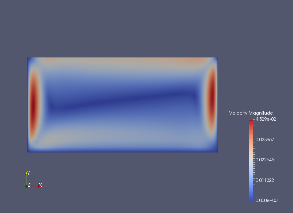
Let us first consider the case without thermophoretic effects (i.e. ).
The flow is driven by buoyancy
forces: the liquid heats up at the left lateral wall inducing an upward flow field that
turns to the right at the top of the container, transporting warm liquid to the right,
cold wall, where it cools down and flows downwards. The cold liquid is flowing back
at the bottom of the container to the left hot wall, see Fig. 1, left picture.
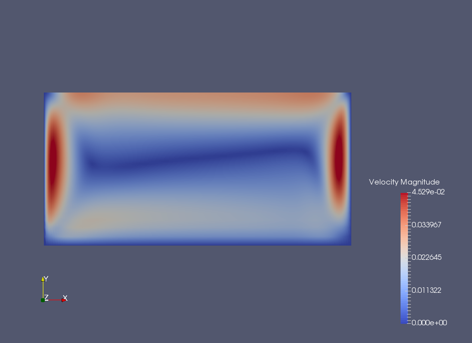
Switching on thermophoretic effects, the flow field is strongly enhanced on the upper
boundary. This can be understood by inspecting the concentration field, see Fig. 2.
The thermophoretic flux
pushes concentration
away from the left, hot and upper walls
(the flux is in direction from hot to cold), thus
decreasing the viscosity there. The opposite effect takes place at the right, cold wall:
concentration is pushed to the cold wall.
Figure 1: Magnitude of velocity without (left) and with (right)
thermophoretic effect (, , ,
, , , ).
Switching on thermophoretic effects, the flow field is strongly enhanced on the upper
boundary.
In order to quantitatively assess the convergence, the same setting as above, however with
different parameters, is used. Since the exact solution is unknown, the computational
solution on a very fine grid with triangles is used as reference instead. Starting from a coarse
triangulation, the grid is successively refined by two bisection steps each. The corresponding
errors and the experimental order of convergence (EOC) are listed in Tab. 1.
As expected one gets a convergence order of 3 (although the boundary of the domain is not of
class ).
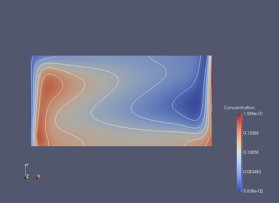
Figure 2: Concentration (, , ,
, , ).
The thermophoretic flux
pushes concentration
away from the left, hot and upper walls
(the flux is in direction from hot to cold), thus
decreasing the viscosity there. The opposite effect takes place at the right, cold wall:
concentration is pushed to the cold wall.
EOC
EOC
EOC
256
3.0296e-04
—
5.3766e-05
—
2.1233e-04
—
1024
2.6758e-05
3.50
5.2109e-06
3.37
2.7126e-05
2.97
4096
2.6659e-06
3.33
5.8438e-07
3.16
3.3971e-06
3.00
16384
3.7459e-07
2.83
7.4084e-08
2.98
4.2396e-07
3.00
Table 1: Errors and EOCs; = number of elements.
, , , , , , .
Acknowledgements
Pedro Morin was partially supported by Agencia Nacional de Promoción Científica y Tecnológica, through grants PICT-2014-2522, PICT-2016-1983, by CONICET through PIP 2015 11220150100661, and by Universidad Nacional del Litoral through grants CAI+D 2016-50420150100022LI. A research stay at Universität Erlangen was partially supported by the Simons Foundation and by the Mathematisches Forschungsinstitut Oberwolfach as well as by the DFG–RTG
2339 IntComSin.
References
[1]
Z. Abbas, R. Perveen, M. Seikh, and I. Pop.
Thermophoretic diffusion and nonlinear radiative heat transfer due to
a contracting cylinder in a nanofluid with generalized slip condition.
Results in Physics, 6:1080–1087, 2016.
[2]
H. Abels.
On a diffuse interface model for two-phase flows of viscous,
incompressible fluids with matched densities.
Arch. Ration. Mech. Anal., 194(2):463–506, 2009.
[3]
L. Ambrosio, A. Carlotto, and A. Massaccesi.
Lectures on elliptic partial differential equations, volume 18
of Appunti. Scuola Normale Superiore di Pisa (Nuova Serie) [Lecture
Notes. Scuola Normale Superiore di Pisa (New Series)].
Edizioni della Normale, Pisa, 2018.
[4]
N. Anbuchezhian, K. Srinivasan, K. Chandrasekaran, and R. Kandasamy.
Thermophoresis and brownian motion effects on boundary layer flow of
nanofluid in presence of thermal stratification due to solar energy.
Appl. Math. Mech.-Engl. Ed., 33:765–780, 2012.
[5]
E. Bänsch.
A thermodynamically consistent model for convective transport in
nanofluids — existence of weak solutions and fem computations.
JMAA, 2019.
[6]
E. Bänsch, S. Faghih-Naini, and P. Morin.
Existence of stationary solutions for a model for convective
transport in nanofluids.
arXiv:1911.04958, 2019.
[7]
S. Brenner and R. Scott.
The mathematical theory of finite element methods, volume 15 of
Texts in Applied Mathematics.
Springer, New York, third edition, 2008.
[8]
J. Buongiorno.
Convective transport in nanofluids.
J. Heat Transfer, 128:240–250, 2006.
[9]
G. Caloz and J. Rappaz.
Numerical analysis for nonlinear and bifurcation problems.
In Handbook of numerical analysis, Vol. V, Handb. Numer.
Anal., V, pages 487–637. North-Holland, Amsterdam, 1997.
[10]
A. Ern and J.-L. Guermond.
Theory and practice of finite elements, volume 159 of Applied Mathematical Sciences.
Springer-Verlag, New York, 2004.
[11]
Y. He, Y. Men, Y. Zhao, H. Lu, and Y. Ding.
Numerical investigation into the convective heat transfer of
nanofluids flowing through a straight tube under the laminar
flow conditions.
Applied Thermal Enginnering, 29:1965–1972, 2009.
[12]
D. Jerison and C. E. Kenig.
The inhomogeneous Dirichlet problem in Lipschitz domains.
J. Funct. Anal., 130(1):161–219, 1995.
[13]
G.S McNab and A. Meisen.
Thermophoresis in liquids.
Journal of Colloid and Interface Science, 44(2):339 – 346,
1973.
[14]
A. Noghrehabadi, A. S. Behbahan, and I. Pop.
Thermophoresis and Brownian effects on natural convection of
nanofluids in a square enclosure with two pairs of heat source/sink with a
nanofluid.
Int. J. Numerical Methods for Heat & Fluid Flow,
25(5):1030–1046, 2015.
[15]
R. Rannacher and R. Scott.
Some optimal error estimates for piecewise linear finite element
approximations.
Math. Comp., 38(158):437–445, 1982.
[16]
R. O. Sayyar and M. Saghafian.
Numerical simualation of convective heat transfer of nonhomogeneous
nanofluid using buongiorno model.
Heat and Mass Transfer, 53:2627–2636, 2017.
[17]
Sh. M. Vanaki, P. Ganesan, and H. A. Mohammed.
Numerical study of convective heat transfer of nanofluids: A review.
Renewable and Sustainable Energy Reviews, 54:1212–1239, 2016.
Eberhard Bänsch Applied Mathematics III University Erlangen–Nürnberg Cauerstr. 11 91058 Erlangen Germany baensch@math.fau.de
Pedro Morin Facultad de Ingeniería Química Universidad Nacional del Litoral and CONICET Santiago del Estero 2829 S3000AOM Santa Fe Argentina pmorin@fiq.unl.edu.ar