Design of Optimal Multiplierless FIR Filters

Abstract

This work presents two novel optimization methods based on integer linear programming (ILP) that minimize the number of adders used to implement a direct/transposed finite impulse response (FIR) filter adhering to a given frequency specification. The proposed algorithms work by either fixing the number of adders used to implement the products (multiplier block adders) or by bounding the adder depth (AD) used for these products. The latter can be used to design filters with minimal AD for low power applications. In contrast to previous multiplierless FIR approaches, the methods introduced here ensure adder count optimality. To demonstrate their effectiveness, we perform several experiments using established design problems from the literature, showing superior results.

I Introduction

FIR filters are fundamental building blocks in digital signal processing (DSP). They provide strict stability and phase linearity, enabling many applications. However, their flexibility typically comes at the expense of a large number of multiplications, making them compute-intensive. Hence, many attempts have been made in the last four decades to avoid costly multiplications and to implement FIR filters in a multiplierless way [1, 2, 3, 4, 5, 6, 7, 8, 9, 10, 11, 12, 13, 14, 15, 16, 17, 18, 19, 20].

One of the most promising ways to do so is to replace constant multiplications by additions, subtractions and bit shifts. Take for example the multiplication by a constant coefficient 23. It can be computed without dedicated multipliers as

$$23x=8\cdot(2x+x)-x=((x<<1)+x)<<3)-x,$$ (1)

where $(x<<b)$ denotes the arithmetic left shift of $x$ by $b$ bits. This computation uses one addition and one subtraction. As the add and subtract operations both have similar hardware cost, the total number of add/subtract units is usually referred to as adder cost. Bit shifts can be hard-wired in hardware implementations and do not contribute any cost. For (1), this is illustrated in Figure 1(a). In general, the task of finding a minimal adder circuit for a given constant is known as the single constant multiplication (SCM) problem and is already an NP-complete optimization problem [21].

Such a problem extends to multiplication with multiple constants, which is necessary when implementing FIR filters. It is called multiple constant multiplication (MCM). Here, some of the intermediate factors like the adder computing $3x$ in Figure 1(a) can be shared among different outputs. Take for example the coefficients $\{7,23\}$; Figure 1(b) shows a solution for multiplying with both coefficients at an adder cost of only two. The corresponding optimization problem is called the MCM problem and has been addressed by numerous heuristic [22, 23, 24] and optimal [25, 26, 27] approaches.

Figure 2 shows the two most popular structures used to implement FIR filters: the direct and transposed forms. The result of an MCM solution can be directly placed in the multiplier block of the transposed form from Figure 2(b). The total adder cost is the sum of the number of multiplier block adders and the remaining ones, commonly called structural adders. The transposed form can be obtained from the direct form by transposition [28]. As the transposition of a single-input-single-output system does not change the adder count, it leads to the same adder cost. So, in the end, it does not matter which one of the two considered filter structures is actually optimized.

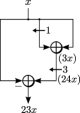
(a) SCM with $23$

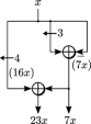
(b) MCM with $\{7,23\}$

Figure 1: Different adder circuits for constant multiplications.

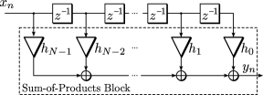
(a) Direct form

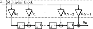
(b) Transposed form

Figure 2: Structure of FIR filters.

In the MCM optimization problem, it is assumed that the coefficients are known and already quantized to a fixed-point (or integer) representation. The design of FIR filters with fixed-point coefficients and a minimum frequency response approximation error is itself a well-known optimization problem, going back to at least [29] (with subsequent extensions and improvements [30, 31, 32, 33, 34]). However, it is often the case in practice that a bounded frequency response is acceptable. In fact, there may be a large number (often hundreds or more) of different fixed-point coefficient sets that meet such a specification. Therefore, a lot of effort in fixed-point FIR filter design has gone into optimizing for resource use. In this context, the problem of finding a minimal adder circuit for a given filter specification was addressed by several authors [1, 2, 4, 5, 7, 9, 15, 19].

However, to the best of our knowledge, no previous work has addressed the design of multiplierless FIR filters in an optimal way. Here, by optimal multiplierless filter we mean a direct/transposed form FIR filter requiring a minimum number of adders to meet a target frequency specification, as well as constraints on the maximum coefficient word size and filter order. The main contributions of our work are as follows:

• We present for the first time a solution for the optimal multiplierless design of FIR filters from a frequency specification using an ILP formulation.

• We provide another ILP formulation that is capable of additionally limiting the adder depth inside the FIR filter.

• We show that relevant problem sizes can be addressed by current ILP solvers and that the adder complexity of well-known FIR filters can be further reduced compared to the most advanced methods.

In the following, we will give background information about previous work this paper is based on. In Section III and Section IV we describe the two ILP formulations that are at the core of the paper, whereas in Section V we talk about ideas meant to improve the practical runtime of the proposed algorithms. We then present experimental results accompanied by a comparison with the state-of-the-art (Section VI), followed by concluding remarks (Section VII).

II Background

Multiplierless filter design problems usually start with a functional specification of the frequency domain behavior, together with the number of filter coefficients and their word lengths. An optimization procedure is applied to get a set of bounded integer coefficients together with their associated adder circuits for the constant multiplications needed in the final implementation. Summarized in Figure 3, this section overviews these parameters and their interactions, together with the state-of-the-art design methods found in the literature.

Figure 3: Simplified multiplierless FIR filter design flow.

II-A Linear Phase FIR Filters

An $N$-th order linear phase FIR filter can be described by its zero-phase frequency response [35]

$$H_{R}(\omega)=\sum_{m=0}^{M-1}h_{m}c_{m}(\omega), \omega\in[0,\pi],$$ (2)

which has the property that its magnitude is identical to that of the transfer function, i.e.,

$$|H(e^{j\omega})|=|H_{R}(\omega)|\ .$$ (3)

The $c_{m}(\omega)$ terms are trigonometric functions and $M$ denotes the number of independent coefficients after removing identical or negated ones due to symmetry. Both depend on the filter symmetry and on the parity of $N$ as given in Table I [35].

Let $\underline{D}(\omega)$ and $\overline{D}(\omega)$ be the desired lower and upper bounds of the output frequency response $H_{R}(\omega)$. The associated frequency specification-based FIR filter design problem consists of finding coefficients $h_{m}$, $m=0,\ldots,M-1$ that fulfill the constraints

$$\underline{D}(\omega) \leqslant H_{R}(\omega)\leqslant\overline{D}(\omega), ~{}\forall\omega\in\Omega,$$ (4)

where $\Omega\subseteq[0,\pi]$ is a set of target frequency bands (usually pass and stopbands). A standard approach in practice is to work with $\Omega_{d}\subseteq\Omega$, a uniform discretization of $\Omega$. One number for the size of $\Omega_{d}$ found in the literature is $16M$ [32].

II-B Fixed-point Constraints

Fixed-point (integer coefficient) FIR filter design problems further restrict the search space to integer variables $h^{\prime}_{m}\in\mathbb{Z}$ with $|h^{\prime}_{m}|<2^{B}$, where the coefficients of $H_{R}(\omega)$ are

$$h_{m}=2^{-B}h^{\prime}_{m}\,$$ (5)

and $B\in\mathbb{N}$ is the maximum effective word length of each coefficient (excluding sign bit).

TABLE I: Relation between filter order $N$, number of coefficients $M$ and function $c_{m}(\omega)$ for different filter types

Type	Sym.	$N$	$M$	$c_{m}(\omega)$
I	sym.	even	$\frac{N}{2}+1$	$c_{m}(\omega)=\begin{cases}1&\text{for }m=0\\ 2\cos(\omega m)&\text{for }m>0\\ \end{cases}$
II	sym.	odd	$\frac{N+1}{2}$	$c_{m}(\omega)=2\cos(\omega(m+1/2))$
III	asym.	even	$\frac{N}{2}$	$c_{m}(\omega)=2\sin(\omega(m-1))$
IV	asym.	odd	$\frac{N+1}{2}$	$c_{m}(\omega)=2\sin(\omega(m+1/2))$

To broaden the feasible set of efficient designs, some applications allow the use of a real-valued scaling factor $G>0$ when computing the quantized fractional coefficients $h_{m}$. Equation (4) thus becomes

$$G\underline{D}(\omega) \leqslant H_{R}(\omega)\leqslant G\overline{D}(\omega), ~{}\forall\omega\in\Omega\ .$$ (6)

When the frequency specification contains a passband, it is called the passband gain [31]. Finding adequate bounds for $G$ is dependent on the set/format of feasible $h_{m}^{\prime}$ coefficient values. If these values are constrained to a power of two space, the ratio between the upper and the lower bound on $G$ does not need to be larger than $2$[31, Lemma 1]. Even when this is not the case, the interval $[0.7,1.4]$ is frequently used [31, 13, 19]. For our tests, unless otherwise stated, we prefer the slightly different interval $[2/3,4/3]$ since it is centered around one. In case a unity or fixed-gain filter is required we set the gain to $G=1$.

II-C Multiplierless FIR Filters

Formulas (5) and (6) are easily expressed as constraints in an ILP formulation. However, to ensure an optimal multiplierless design, further constraints are needed.

The way these constraints are constructed and used has varied over the years. Early research in this direction looked at multiplierless designs where each coefficient was represented by a limited number of signed power-of-two terms, optimized using branch-and-bound techniques [1]. Later, minimum signed digit (MSD) representations characterized by a minimum number of non-zero power-of-two terms were quickly adopted for this purpose [2, 5, 6, 10, 15].

MSD representations can be used to find sharing opportunities of intermediate computations like the $7x$ term shown in Figure 1(b). One way is by searching and eliminating redundant bit patterns common to several coefficients, a technique called common subexpression elimination (CSE). Savings are obtained by performing the computation specified by the bit pattern and distributing the result to all coefficients depending on it [22, 3, 7, 8]. However, the CSE search cannot deliver all possible sharing opportunities due to its dependency on the number representation [23] and the effect of hidden non-zeros [36]. To avoid them, graph-based approaches are commonly used in state-of-the-art MCM methods [22, 23, 24, 25, 26, 27]. Some early work on multiplierless FIR filter design already considered this by incorporating the graph-based MCM algorithm of [22] into a genetic algorithm that optimizes the filter coefficients according to the adder cost [4]. A different approach is followed by [9], where a branch-and-bound-based ILP optimization is used; here, a pre-specified set of integer terms, called the subexpression space, has to be provided that can be shared among the different coefficient expansions. This work was later extended with a dynamic subexpression space expansion algorithm [11, 13], which, at least in the case of [13], claims to usually produce designs with a minimal number of adders. In contrast to these potentially slow branch-and-bound approaches, in [16], a fast polynomial-time heuristic for the design of low complexity multiplierless linear-phase FIR filters was proposed.

Recent work has also focused on integrating filter coefficient sparsity, which can also have a big impact on the complexity of the final design [17] by reducing the number of structural adders. Also, other structures than the direct and transposed forms (see Figure 2) have been shown to possess good properties. The factoring of FIR filters into a cascade of relatively small subsections can lead to a lower bit-level complexity [14, 18]. Alternative structures have also been proposed [20]; they provide lower word sizes for the structural adders.

Besides optimizing the adder count, it was shown early that the power consumption of the resulting filter also strongly depends on the adder depth (AD), which is defined as the number of cascaded adders in the multiplier block [37, 38]. Since then, many works have focused on limiting the AD either in MCM algorithms [39, 36, 40] or directly in multiplierless filter design methods [13]. Again, all of those approaches are heuristics that provide minimal AD but not guarantee minimal adder cost. Looking at the average adder depth in the structural adders can also help reduce power consumption [19].

III Multiplierless FIR Filters with Fixed Number of Multiplier Block Adders

Our first ILP model targets the design of generic multiplierless FIR filters regardless of their adder depth. It is based on a recently proposed MCM ILP formulation [27], where the goal is to directly compute the parameters of an MCM adder graph, if feasible, for a given number of adders. This idea is extended here for multiplierless FIR filter design by adding constraints on the frequency specification. As a result, we get an ILP model to design a multiplierless filter for a fixed number of adders in the multiplier block. To optimize the total number of adders, this ILP model is solved several times using an overall algorithm discussed in Section III-B. In the following, we first present the ILP formulation for the fixed number of multiplier block adders.

III-A ILP Formulation for Fixed Multiplier Block Adder Count

The proposed ILP formulation is given in ILP Formulation 1 and uses the constants and variables listed in Table II. The objective is, given a fixed number of multiplier block adders $A_{\text{M}}$, to minimize the number of structural adders $A_{\text{S}}$ (which depend on the number of zero filter coefficients, encoded by the binary decision variables $h_{m,0}$).

The resulting constraints can be roughly divided into frequency response conditions (C1, C2), equations linking the filter coefficients with the coefficients of the multiplier block (C3) and formulas describing the multiplierless realization of the multiplier block (C4 – C8).

The integer coefficients $h^{\prime}_{m}$ ($m=0,\ldots,M-1$) of the FIR filter are directly used as integer variables in the ILP formulation. The resulting frequency response is constrained in C1a by setting (2) and (5) into (6). Constraints C1b are so-called lifting constraints. These are actually not required to solve the problem, but can significantly reduce the search space and improve runtime performance. Specifically, they limit the range of the coefficients to lower $\underline{h_{m}}$ and upper $\overline{h_{m}}$ bounds. The computation of these bounds is considered in Section V-A. Constraint C2 limits the range of the gain as discussed in Section II.

Constraints C3a to C3c provide the connection between the filter coefficient $h^{\prime}_{m}$ and the (potentially shifted and sign-corrected) multiples computed in the multiplier block $c_{a}$ or a zero coefficient. For that, the binary decision variables $o_{a,m,s,\phi}\in\{0,1\}$ encode if $h^{\prime}_{m}$ is connected to adder $a$ of the multiplier block, shifted by $s$, and either added ($\phi=0$) or subtracted ($\phi=1$) in the structural adders (C3a). In case the coefficient is zero, a single binary decision variable $h_{m,0}$ is used (C3b). This encoding allows the optimization of structural adders by considering the $h_{m,0}$ variables in the objective function. For every zero coefficient, the corresponding structural adder(s) can be saved depending on the coefficient and filter type. Table III shows the number of structural adders for the different filter types. Overall, constraints C3c ensure that only one of the above cases is valid.

ILP Formulation 1 Multiplierless FIR filters with fixed $A_{\text{M}}$

$$\text{minimize}\ A_{\text{S}}(h_{m,0})$$

subject to

C1a: $$G2^{B}\underline{D}(\omega)\leqslant\sum_{m=0}^{M-1}h^{\prime}_{m}c_{m}(\omega)\leqslant G2^{B}\overline{D}(\omega),~{}\forall\omega\in\Omega_{d}$$

C1b: $$\underline{h_{m}}\leqslant h^{\prime}_{m}\leqslant\overline{h_{m}},~{}\forall m=0,\ldots,M-1$$

C2: $$2/3\leqslant G\leqslant 4/3$$

C3a: $$h^{\prime}_{m}=(-1)^{\phi}2^{s}c_{a}\text{ if }o_{a,m,s,\phi}=1$$

$$~{}\forall a=0,\ldots,A_{\text{M}},m=0,\ldots,M-1$$

C3b: $$h^{\prime}_{m}=0\text{ if }h_{m,0}=1,~{}\forall m=0,\ldots,M-1$$

C3c: $$\sum_{a=0}^{A_{\text{M}}}\sum_{s=S_{\text{min}}}^{S_{\text{max}}}\sum_{\phi=0}^{1}o_{a,m,s,\phi}+h_{m,0}=1,~{}\forall m=0,\ldots,M-1$$

C4: $$\hskip 42.67912ptc_{0}=1$$

C5: $$c_{a}=c^{\text{sh,sg}}_{a,\ell}+c^{\text{sh,sg}}_{a,\text{r}},~{}\forall a=1,\ldots,A_{\text{M}}$$

C6a: $$c_{a,i}=c_{k}\text{ if }c_{a,i,k}=1,~{}\forall a=1,\ldots,A_{\text{M}},i\in\{\ell,\text{r}\}$$

$$k=0,\ldots,a-1$$

C6b: $$\sum_{k=1}^{a-1}c_{a,i,k}=1,~{}\forall a=1,\ldots,A_{\text{M}},i\in\{\ell,\text{r}\}$$

C7a: $$c^{\text{sh}}_{a,i}=2^{s}c_{a,i}\text{ if }\varphi_{a,i,s}=1$$

$$~{}\forall a=1,\ldots,A_{\text{M}},i\in\{\ell,\text{r}\},s=S_{\text{min}},\ldots,S_{\text{max}}$$

C7b: $$\sum_{s=S_{\text{min}}}^{S_{\text{max}}-1}\varphi_{a,i,s}=1,~{}\forall a=1,\ldots,A_{\text{M}},i\in\{\ell,\text{r}\}$$

C7c: $$\varphi_{a,\ell,s}=0~{}\forall s>0$$

C7d: $$\varphi_{a,\ell,s}=\varphi_{a,\text{r},s}~{}\forall s<0$$

C8a: $$c^{\text{sh,sg}}_{a,i}=-c^{\text{sh}}_{a,i}\text{ if }\phi_{a,i}=1,~{}\forall a=1,\ldots,A_{\text{M}},i\in\{\ell,\text{r}\}$$

C8b: $$c^{\text{sh,sg}}_{a,i}=c^{\text{sh}}_{a,i}\text{ if }\phi_{a,i}=0,~{}\forall a=1,\ldots,A_{\text{M}},i\in\{\ell,\text{r}\}$$

C8c: $$\phi_{a,\ell}+\phi_{a,\text{r}}\leqslant 1,~{}\forall a=1,\ldots,A_{\text{M}}$$

TABLE II: Used constants (top) and variables (bottom) in ILP Formulation 1

Constant/Variable	Meaning
$A_{\text{M}}\in\mathbb{N}$	Number of adders in the multiplier block
$M\in\mathbb{N}$	Number of filter coefficients
$S_{\text{min}}$, $S_{\text{max}}\in\mathbb{Z}$	Minimum and maximum shift
$A_{\text{S}}\in\mathbb{N}$	Number of structural adders
$h^{\prime}_{m}\in\mathbb{Z}$	Integer representation of filter coefficient
$h_{m,0}\in\{0,1\}$	true, if coefficient $h^{\prime}_{m}$ is zero
$c_{a}\in\mathbb{N}$	Constant computed in adder $a$
$c_{a,i}\in\mathbb{N}$	Constant of input $i\in\{\ell,\text{r}\}$ of adder $a$
$c^{\text{sh}}_{a,i}\in\mathbb{N}$	Shifted constant of input $i\in\{\ell,\text{r}\}$ of adder $a$
$c^{\text{sh,sg}}_{a,i}\in\mathbb{N}$	Shifted, sign corrected constant of input $i\in\{\ell,\text{r}\}$ of adder $a$
$\phi_{a,i}\in\{0,1\}$	Sign of input $i\in\{\ell,\text{r}\}$ of adder $a$ (0:’$+$’, $1$:’$-$’)
$c_{a,i,k}\in\{0,1\}$	true, if input $i$ of adder $a$ is connected to adder $k$
$\varphi_{a,i,s}\in\{0,1\}$	true, if input $i$ of adder $a$ is shifted by $s$ bits
$o_{a,m,s,\phi}\in\{0,1\}$	true, if coefficient $h^{\prime}_{m}$ is connected to adder $a$, shifted by $s$ and sign $\phi$
$\underline{h_{m}},\overline{h_{m}}\in\mathbb{Z}$	Lower and upper bound for filter coefficient $m=0\ldots M-1$
$G\in[2/3,4/3]$	Gain of a variable gain filter ($G=1$ when the gain is fixed)

The remaining constraints C4 – C8 are identical to the ones used for solving the MCM problem from [27]. We give a brief description here, but refer the reader to [27] for a more detailed presentation. The multiplier block input is viewed as a multiplication by factor one ($c_{0}=1$) and is defined with constraint C4. Constraints C5 represent the actual add operation of adder $a$ and its corresponding factor $c_{a}$. It is obtained by adding the shifted and possibly sign corrected factors of its left input $c^{\text{sh,sg}}_{a,\ell}$ and its right input $c^{\text{sh,sg}}_{a,\text{r}}$. The source of the adder inputs is encoded by C6a/b. Indicator constraints C6a are used to set the value $c_{a,i}$ of the adder input $i\in\{\ell,\text{r}\}$ to the actual factor when the corresponding decision variable $c_{a,i,k}$ is set. Indicator constraints are special constraints in which a binary variable controls whether or not a specified linear constraint is active. They are in-fact non-linear but supported by many modern ILP solvers and are also simple to linearize for other solvers (see [27]). Constraints C6b make sure that only one source is selected. The actual shift is constrained by C7a/b in a similar way: indicator constraints C7a are used to set the shifted factor $c^{\text{sh}}_{a,i}$ according to the corresponding decision variable $\varphi_{a,i,s}$.

Constraints C7c and C7d are both optional lifting constraints used to reduce the search space. As the filter coefficients can be shifted in constraint C3a, we can limit the constants of the multiplier block to odd numbers. This allows us to use the well-known fact that odd coefficients can be computed from odd numbers using one addition with either one operand left shifted while the other operand is not shifted or both operands are right shifted by the same value [41, Theorem 3].

To support subtractions, indicator constraints C8a/b are used to set the sign according to decision variable $\phi_{a,i}$. Finally, constraints C8c ensure that at most one input of the adder can be nagative, as subtracting both inputs is typically more hardware demanding.

All of the integer variables from Table II are computed from integer constants or booleans and represent integer values. So they can be relaxed to real numbers to speed up the optimization.

TABLE III: Number of structural adders for the different filter types

Type	no. of structural adders, $A_{\text{S}}(h_{m,0})$
I	$\displaystyle N-h_{0,0}-2\sum_{m=1}^{M-1}h_{m,0}$
II	$\displaystyle N-2\sum_{m=0}^{M-1}h_{m,0}$
III	$\displaystyle N-2\sum_{m=1}^{M-1}h_{m,0}$
IV	$\displaystyle N-2\sum_{m=0}^{M-1}h_{m,0}$

III-B Minimizing the Total Number of Adders

As the number of adders in the multiplier block $A_{\text{M}}$ is fixed in ILP Formulation 1, we need to iterate over various values $A_{\text{M}}$ to find the minimum number of total adders

$$A=A_{\text{M}}+A_{\text{S}}\ .$$ (7)

For that, we first search for a solution with minimal number of multiplier block adders by solving ILP Formulation 1 for $A_{\text{M}}=0,1,2,\ldots$ until we obtain the first feasible solution.

This solution with minimum multiplier block adders $A_{\text{M,min}}$ is not necessarily the global optimum as there might be a solution with $A_{\text{M}}>A_{\text{M,min}}$ and a smaller $A_{\text{S}}$. To account for this, we need a lower bound for the structural adders $A_{\text{S,min}}$. This is obtained once at the beginning of the overall algorithm by solving the problem for a maximally sparse FIR filter, which we do by taking ILP Formulation 1 where only the constraints C1 – C3 are considered.

In case the structural adders $A_{\text{S}}$ of solution with $A_{\text{M}}=A_{\text{M,min}}$ are not identical with $A_{\text{S,min}}$, we continue to further increment $A_{\text{M}}$ until we find a solution with $A_{\text{S}}=A_{\text{S,min}}$. This is a safe stopping point since, by the optimality of ILP Formulation 1, there is no solution with larger $A_{\text{M}}$ and smaller $A_{\text{S}}$. The solution with minimum total adders $A$ found so far is hence also globally optimal. Typically, only a few iterations are necessary to reach this point.

IV Multiplierless FIR Filters with Bounded Adder Depth

As discussed above, limiting the AD is important to reduce the power consumption of a filter. Unfortunately, adapting ILP Formulation 1 to limit the AD is not straightforward, as the topology of the adders and thus the AD is left open. We present in this section a novel ILP model for the design of multiplierless FIR with limited AD which is based on a formulation that was initially designed for optimizing pipelined MCM (PMCM) circuits [42, 40].

In contrast to ILP Formulation 1, the possible coefficients are precomputed for each adder stage $s$ and selected using binary decision variables. The computation of the corresponding coefficient sets is given next.

IV-A Definition of Coefficient Sets

We use some notation and definitions originally introduced in [23]. First, we define the generalized add operation called $\mathcal{A}$-operation, which includes the shifts. An $\mathcal{A}$-operation has two input coefficients $u,v\in\mathbb{N}$ and computes

$$\mathcal{A}_{q}(u,v)=|2^{l_{u}}u+(-1)^{s_{v}}2^{l_{v}}v|2^{-r},$$ (8)

where $q=(l_{u},l_{v},r,s_{v})$ is a configuration vector which determines the left shifts $l_{u},\ l_{v}\in\mathbb{N}_{0}$ of the inputs, $r\in\mathbb{N}_{0}$ is the output right-shift and $s_{v}\in\{0,1\}$ is a sign bit which denotes whether an addition or subtraction is performed.

Next, we define the set $\mathcal{A}_{*}(u,v)$ containing all possible coefficients which can be obtained from $u$ and $v$ by using exactly one $\mathcal{A}$-operation:

$$\mathcal{A}_{*}(u,v):=\{\mathcal{A}_{q}(u,v)\ |\ q\text{ is a valid configuration}\}\ .$$ (9)

A valid configuration is a combination of $l_{u}$, $l_{v}$, $r$ and $s_{v}$ such that the result is a positive odd integer $\mathcal{A}_{q}(u,v)\leqslant c_{\max}$. The reason for limiting the integers to odd values is that we can compute every even multiple by shifting the corresponding odd multiple to the left. The $c_{\max}$ limit is used to keep $\mathcal{A}_{*}(u,v)$ finite. It is chosen as a power-of-two value which is usually set to the maximum coefficient bit width $B$ plus one [23, 22]

$$c_{\max} :=2^{B+1}\ .$$ (10)

For convenience, the $\mathcal{A}_{*}$ set is also defined for an input set $X\subseteq\mathbb{N}$ as

$$\mathcal{A}_{*}(X):=\bigcup_{u,v\in X}\mathcal{A}_{*}(u,v)\ .$$ (11)

We can now define the coefficients that can be computed at adder stage $s$, denoted as $\mathcal{A}^{s}$, by recursively computing the $\mathcal{A}_{*}$ sets

$$\mathcal{A}^{0} :=\{1\}$$ (12)

$$\mathcal{A}^{s} :=\mathcal{A}_{*}(\mathcal{A}^{s-1})\ .$$ (13)

In addition, let $\mathcal{T}^{s}$ denote the set of $(u,v,w)$ triplets for which $w\in\mathcal{A}^{s}$ can be computed using $u$ and $v$ from the previous stage (i.e., $u,v\in\mathcal{A}^{s-1}$). $\mathcal{T}^{s}$ can be computed recursively, starting from the last stage $s$, which is equal to the maximum allowable AD:

$$\mathcal{T}^{s}:=\{(u,v,w)\ | \ w=\mathcal{A}_{q}(u,v),$$

$$u,v\in\mathcal{A}^{s},\ u\leqslant v,\ w\in\mathcal{A}^{s+1}\}.$$ (14)

To give an example, the first elements of $\mathcal{T}^{1}$ are $\mathcal{T}^{1}=\{(1,1,1),(1,1,3),(1,1,5),(1,1,7),(1,1,9),(1,1,15),\ldots\}$. This set contains all the possible rules for computing multiples from the input within one stage of additions, while set $\mathcal{T}^{2}=\mathcal{T}^{1}\cup\{(1,3,11),(1,5,11),\ldots,(3,5,11),\ldots\}$ contains all the combinations of how elements in the next stage can be computed.

IV-B ILP Formulation for Fixed Adder Depth

The bounded AD model is given in ILP Formulation 2, while the corresponding constants and variables are given in Table IV.

In contrast to ILP Formulation 1, the objective is to directly minimize the total number of adders $A$, which is separated into adders in the multiplier block ($A_{\text{M}}$) and structural adders $A_{\text{S}}$. Similar to ILP Formulation 1, the constraints are divided into frequency response conditions (C1, C2), the link between the filter coefficients and the coefficients of the multiplier block (C3, C4) and the equations describing the multiplierless realization of the multiplier block (C5 – C8).

ILP Formulation 2 Multiplierless FIR filters with depth limit

$$\text{minimize}\ \underbrace{\sum_{s=1}^{S}\sum_{w\in\mathcal{A}^{s}}a_{w}^{s}}_{=A_{\text{M}}}+A_{\text{S}}(h_{m,0})$$

subject to

C1a: $$G2^{B}\underline{D}(\omega)\leqslant\sum_{m=0}^{M-1}h^{\prime}_{m}c_{m}(\omega)\leqslant G2^{B}\overline{D}(\omega),~{}\forall\omega\in\Omega_{d}$$

C1b: $$\underline{h_{m}}\leqslant h^{\prime}_{m}\leqslant\overline{h_{m}},~{}\forall m=0,\ldots,M-1$$

C2: $$2/3\leqslant G\leqslant 4/3$$

C3a: $$h^{\prime}_{m}=\begin{cases}\displaystyle\sum_{w=0}^{2^{B}-1}wh_{m,w}&\text{ if }\phi_{m}=0\\ \displaystyle-\sum_{w=1}^{2^{B}-1}wh_{m,w}&\text{ if }\phi_{m}=1\\ \end{cases}$$

$$~{}\forall m=0,\ldots,M-1$$

C3b: $$\sum_{w=0}^{2^{B}-1}h_{m,w}=1,~{}\forall m=0,\ldots,M-1$$

C4: $$r_{\textnormal{odd}(w)}^{S}+a_{\textnormal{odd}(w)}^{S}\geqslant\frac{1}{M}\sum_{m=0}^{M-1}h_{m,w},~{}\forall w=0,\ldots,2^{B}-1$$

C5: $$r_{w}^{s}=0~{}\forall w\in\mathcal{A}^{s}\setminus\bigcup_{s^{\prime}=0}^{s-1}\mathcal{A}^{s^{\prime}}\text{ with }s=1,\ldots,S-1$$

C6: $$r_{w}^{s}-a_{w}^{s-1}-r_{w}^{s-1}\leqslant 0,~{}\forall w\in\mathcal{A}^{s}\setminus\{0\}\text{, }s=2,\ldots,S$$

C7: $$a_{w}^{s}-\sum_{(u,v,w^{\prime})\in\mathcal{T}^{s}\,|\,w^{\prime}=w}x_{(u,v)}^{s-1}\leqslant 0$$

$$~{}\forall w\in\mathcal{A}^{s},s=2,\ldots,S$$

C8: $$\begin{aligned} x_{(u,v)}^{s}-r_{u}^{s}-a_{u}^{s}\leqslant 0\\ x_{(u,v)}^{s}-r_{v}^{s}-a_{v}^{s}\leqslant 0\\ \end{aligned}$$

$$~{}\forall(u,v,w)\in\mathcal{T}^{s}\text{ with }s=1,\ldots,S-1$$

Constraints C1a/b and C2 are identical to the ones in ILP Formulation 1. Now, the connection between the odd multiplier block coefficients of the pre-computed sets and the filter coefficients is performed using binary decision variables. Let $h_{m,w}\in\{0,1\}$ be a binary decision variable that is true if the magnitude of $h^{\prime}_{m}$ is identical to $w$, i.e.,

$$h_{m,w}=\begin{cases}1&\text{when }|h^{\prime}_{m}|=w\\ 0&\text{otherwise}\\ \end{cases}$$ (15)

for $m=0,\ldots,M-1$ and $w=0,\ldots,2^{B}-1$. Furthermore, let $\phi_{m}$ determine the sign of $h^{\prime}_{m}$ as follows

$$\phi_{m}=\begin{cases}0&\text{when }h^{\prime}_{m}\geq 0\\ 1&\text{otherwise}\ .\\ \end{cases}$$ (16)

The value of each integer coefficient $h^{\prime}_{m}$ is selected by the indicator constraints C3a. In addition, constraints C3b make sure that only one value per filter coefficient is selected.

Next, we distinguish between coefficients that are computed for the selected stage (by using an addition) and coefficients that are just replicated from a previous stage. This replication can be either implemented by a simple wire (as this was implied in ILP Formulation 1) or in case of a pipelined implementation of the multiplier block, it will be implemented by a register. This allows to also model the register cost in the latter case (not treated here but it is a trivial extension of the objective). Hence, we introduce two new decision variables for each $w$ and stage: $a_{w}^{s}$ and $r_{w}^{s}$, which are true, if $w$ in stage $s$ is realized using an adder or register/wire, respectively.

The connection to the filter coefficients $h_{m,w}$ is made through C4. As several of the $M$ $h_{m}$ coefficients can have the same $w$ value, the right hand side of C4 is scaled by $1/M$ to keep it less than one. Whenever the right hand side of C4 is non-zero it forces the realization of coefficient $w$ in the output stage $S$, either as an adder or as a register/wire.

TABLE IV: Used constants (top) and variables (bottom) in ILP Formulation 2

Constant/Variable	Meaning
$M\in\mathbb{N}$	Number of filter coefficients
$\mathcal{A}^{s}\subseteq\mathbb{N}$	Coefficients that can be computed in adder stage $s$
$\mathcal{T}^{s}\subseteq\mathbb{N}^{3}$	Tripplets $(u,v,w)$ from which $w\in\mathcal{A}^{s}$ can be computed using $u,v\in\mathcal{A}^{s-1}$
$\underline{h_{m}},\overline{h_{m}}\in\mathbb{Z}$	Lower and upper bound for filter coefficient $m=0,\ldots,M-1$
$h^{\prime}_{m}\in\mathbb{Z}$	Value of filter coefficient $m=0,\ldots,M-1$
$h_{m,w}\in\{0,1\}$	true, if $|h^{\prime}_{m}|=w$ for $m=0,\ldots,M-1$ and $w=0,\ldots,2^{B}-1$
$\phi_{m}\in\{0,1\}$	true, if $h^{\prime}_{m}$ is negative
$a_{w}^{s}\in\{0,1\}$	true, if $w\in\mathcal{A}^{s}$ in stage $s=1,\ldots,S-1$ is realized using an adder
$r_{w}^{s}\in\{0,1\}$	true, if $w\in\mathcal{A}^{s}$ in stage $s=1,\ldots,S-1$ is realized using a register or wire
$x^{s}_{(u,v)}\in\{0,1\}$	true, if $u$ and $v$ are available in stage $s=1,\ldots,S-2$
$G\in[2/3,4/3]$	Gain of a variable gain filter ($G=1$ when the gain is fixed)

Constraints C5 and C6 consider the realization as register/wire: they require that a value $w$ can only be replicated from a previous stage if it was computed or replicated before.

The realization as an adder computing constant $w$ from the inputs $u$ and $v$ requires the presence of both inputs in the previous stage. For that, the binary variables $x_{(u,v)}^{s}$ are introduced which determine if both are available in stage $s$:

$$x_{(u,v)}^{s}=\begin{cases}1&\text{if both $u$ and $v$ are available in stage $s$}\\ 0&\text{otherwise}\end{cases}$$ (17)

Now, constraint C7 specifies that if $w$ is computed by $w=\mathcal{A}(u,v)$ in stage $s$, the pair $(u,v)$ has to be available in the previous stage. If a pair ($u,v$) is required in stage $s$, constraints C8 make sure that $u$ and $v$ have been realized in the previous stage either as register or adder.

Note that instead of using constraint C5 it is more practical to remove all variables $r_{w}^{s}$ which are zero from the cost function and their related constraints. Also note that the binary variables $x^{s}_{(u,v)}$ and the integer variables $h_{m}$ can be relaxed to real numbers to speed up the optimization.

IV-C Selecting the Adder Depth

The AD is often selected to be as small as possible, typically at the expense of a higher adder cost. It is well known that the minimal AD needed when multiplying with a given coefficient can be realized by using a binary tree [43]. Therefore, it cannot be lower than the base two logarithm of the non-zero digit count of its MSD representation. Unfortunately, as the coefficients are not known in advance, the minimum AD cannot be derived from the filter specification. However, the upper bound of the AD can be computed from the coefficient word size $B$ as follows. A $B$ bit binary number can have up to $B+1$ digits when represented as an MSD number and up to $\lfloor{(B+1)/2}\rfloor+1$ non-zeros in the worst case [40]. This leads to a maximum adder depth of

$$\text{AD}_{\max}=\log_{2}\left(\left\lfloor\frac{B+1}{2}\right\rfloor+1\right)\ .$$ (18)

Using this bound, a search from $\text{AD}=0,\ldots,\text{AD}_{\max}$ can be performed until the first feasible solution is found.

For practical FIR filters, early studies have shown that coefficient word sizes between 15 bit to 20 bit are sufficient to achieve approximation errors between $-70$ and $-100$ dB [44]. Using (18), this translates to ADs of at most three to four. In our experiments, we found very good solutions with $\text{AD}=2$ for most of the filters from practice.

V Reducing the Problem Complexity

V-A Reducing the Coefficient Range

Following [5, Sec. 4], we bound the search space for the coefficient values by projecting the polytope corresponding to the discretized versions of (4) or (6) onto each $h_{m}^{\prime}$. The goal is a tight interval enclosure $[\underline{h_{m}},\overline{h_{m}}]$ for the feasible values of $h_{m}^{\prime}$. This corresponds to the LPs:

$$\text{minimize}\ h_{m}^{\prime}$$

or

$$\text{maximize}\ h_{m}^{\prime}$$

subject to

$$G\underline{D}(\omega)\leqslant\sum_{k=0}^{M-1}h_{k}^{\prime}c_{k}(\omega)\leqslant G\overline{D}(\omega),\quad~{}\forall\omega\in\Omega_{d},$$

where $h_{k}^{\prime}\in\mathbb{R}$ for $k=0,\ldots,M-1$ and $G\in\left[2/3,4/3\right]$ (or $G=1$ when unity gain is used). We get $[\underline{h_{m}},\overline{h_{m}}]$ by taking

$$\underline{h_{m}} =\left\lceil h_{m}^{\prime}\right\rceil\text{ from minimize }h_{m}^{\prime},$$

$$\overline{h_{m}} =\left\lfloor h_{m}^{\prime}\right\rfloor\text{ from maximize }h_{m}^{\prime}.$$

V-B Discretizing the Frequency Domain

Even though $\Omega$ is replaced by a finite set $\Omega_{d}$, we perform a rigorous posteriori validation of the result over $\Omega$ [45]. Still, the typically large size of $\Omega_{d}$ ($16M$ is a common value found in the literature) can have a big impact on the runtime of the filter design routine. This is shown for instance in the context of an optimal branch-and-bound algorithm for FIR filter design with fixed-point coefficients [32, Table 2]. A too small number of points can, on the other hand, lead to an invalid solution over $\Omega$ and a larger feasible set, potentially incurring a larger runtime as well.

It is thus important to consider a discretization of reasonable size that is unlikely to lead to invalid solutions over $\Omega$ (i.e., equations (4) or (6) do not hold) and does not increase the search space by a too large factor. To this effect, we use so-called approximate Fekete points (AFPs), which contain the most critical frequencies for a given filter that needs to fit a target frequency response. They have recently been used to improve the robustness of the classic Parks-McClellan Chebyshev FIR filter design algorithm [46] and for a fast and efficient heuristic for FIR fixed-point coefficient optimization [47]. They are efficient choices when performing polynomial interpolation/approximation on domains such as $\Omega$. This is relevant in our context since $H_{R}(\omega)$ in (2) is a polynomial in $\cos(\omega)$ [48, Ch. 7.7]. For details on how to compute them we refer the reader to [46, 47] and the references therein.

V-C An Adaptive Search Strategy

Even if the current $\Omega_{d}$ leads to a solution that does not pass a posteriori validation, it might still be possible to rescale the gain factor $G$ such that (6) holds. By taking a point $\omega_{\max}\in\Omega$ where $G\underline{D}(\omega_{\max})-H_{R}(\omega_{\max})$ or $H_{R}(\omega_{\max})-G\overline{D}(\omega_{\max})$ is largest (i.e., the point of largest deviation from the specification) we first update $G$ to take a value close to $H_{R}(\omega_{\max})/\underline{D}(\omega_{\max})$ or $H_{R}(\omega_{\max})/\overline{D}(\omega_{\max})$, depending on where the deviation occurs. If this new gain leads to a valid solution over $\Omega$, then it is optimal. If not, we update $\Omega_{d}$ by adding the points of largest deviation for each frequency subdomain. We rerun the optimization with this new $\Omega_{d}$, repeating until either (a) there are no more invalid frequency points or (b) the problem becomes infeasible, meaning no solution with the imposed constraints over $\Omega$ exists.

We should mention that running the result validation code of [45] at each iteration of the adaptive routine is computationally expensive. This is why at each iteration we perform a fast, non rigurous test consisting of verifying (6) on a much denser discretization of $\Omega$ than $\Omega_{d}$. We found this to usually be sufficient in ensuring that the a posteriori validation [45] done at the end of optimization is successful.

VI Experimental Results

To test the ILP formulations discussed above, we have implemented them in a C++ filter design tool. It features a flexible command-line interface.

VI-A Experimental Setup and Parameter Choices

All experiments were run on a Linux machine with an Intel Xeon E5-2690 v4 CPU with 56 cores and 252 GB of RAM. The proposed implementation supports several popular open source and commercial (M)ILP solvers, such as SCIP [49], Gurobi [50] and CPLEX [51]. For convenience, these solvers are accessed through the ScaLP [52] library, which acts as a frontend. Based on our experiments, Gurobi usually proved to be the fastest backend, which is why, apart from a few exceptions, use it on all the examples below.

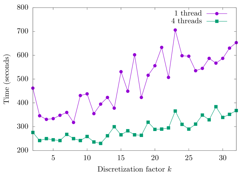
Figure 4: Total execution times for the design of a family of filters from Section VI-B1 with respect to the size of $\Omega_{d}$ ($kM$ points). Each data point corresponds to the time for the design of 42 filters of increasing complexity.

All experiments use the AFP-based frequency grid discretization mentioned in Section V-B. As discussed before, the number of frequency points in $\Omega_{d}$ is run-time critical. To determine an appropriate size, we ran an experiment using a typical design scenario with an $\Omega_{d}$ size of $kM$ points and $k=1,\ldots,32$. Figure 4 shows the runtimes. Not surprisingly, they start large for very low $k$, as in these cases the frequency grid usually has to be extended to address violations, which require re-running the optimization routine on a new grid. As soon as $k$ is large enough (around $k\geqslant 4$), invalid results become rare, meaning just one optimization pass is sufficient. Further increasing $k$ at this point just leads to more constraints in the model and likely a larger runtime for the optimizer. Based on these results, we selected to start with $4M$ points. We find this choice usually delivers a good balance between optimizer runtime and number of iterations needed to obtain a valid solution over $\Omega$.

TABLE V: Specifications of the reference filters

(a) Specifications S1, S2, L1, L2 and their variations.

Name	Source	$\Omega_{p}/\pi$	$\Omega_{s}/\pi$	$\delta_{p}$	$\delta_{s}$
S1a	[2]	$[0,0.3]$	$[0.5,1]$	$0.00645$	$0.00645$
S1b	[4]	$[0,0.3]$	$[0.5,1]$	$0.00636$	$0.00636$
S1c	[9, 13]	$[0,0.3]$	$[0.5,1]$	$0.01570$	$0.00660$
S2a	[2, 10]	$[0,0.042]$	$[0.14,1]$	$0.01160$	$0.001$
S2b	[9, 13]	$[0,0.042]$	$[0.14,1]$	$0.01200$	$0.001$
L1	[10, 9]	$[0.8,1]$	$[0,0.74]$	$0.0057$	$0.0001$
L2	[1, 15]	$[0,0.2]$	$[0.28,1]$	$0.02800$	$0.001$

(b) Specification of the multiband filter L3.

$\Omega_{i}/\pi$	$\underline{D}(\omega)$	$\overline{D}(\omega)$
$[0,0.15]$	$0.9772$	$1.0232$
$[0.15,0.1875]$	$0.9441$	$1.0232$
$[0.1875,0.2125]$	$0.9016$	$1.0232$
$[0.2875,1]$	$0$	$0.0316$

VI-B Benchmark Set

Several multiplierless filter designs were computed to evaluate our methods. They are introduced next.

VI-B1 A Family of Specifications from [4, Example 1]

We consider a family of low-pass linear-phase filter specifications from Redmill et al. [4]. These specifications are defined by:

$$1-\delta \leqslant H_{R}(\omega)\leqslant 1+\delta, \omega\in[0,0.3]\quad\text{(passband)}$$

$$-\delta \leqslant H_{R}(\omega)\leqslant\delta, \omega\in[0.5,0.1]\quad\text{(stopband)}$$

where $\delta$ is a parameter regulating error. We set ${\delta=10^{-\frac{p}{20}}}$, where $p>0$ is the error in decibels (dB).

Our goal with this benchmark is to explore the tradeoff between the error ($p$), the filter order ($N$) and the word length ($B$) in terms of the total number of adders.

VI-B2 A Set of State-of-the-art Specifications

We also test our tool on a set of reference specifications from the literature [1, 2, 4, 9, 12, 13, 15], referred to as $S1$, $S2$, $L1$, $L2$ and $L3$. They are all low-pass filters defined by

$$1-\delta_{p} \leqslant H_{R}(\omega)\leqslant 1+\delta_{p}, \omega\in\Omega_{p}\quad\text{(passband)},$$

$$-\delta_{s} \leqslant H_{R}(\omega)\leqslant\delta_{s}, \omega\in\Omega_{s}\quad\text{(stopband)},$$

where the values of $\delta_{p},\delta_{s},\Omega_{p},\Omega_{s}$ for each specification are given in Table V. Over time, these reference filter specifications were slightly modified by different publications. To compare with each one, we indicate variations by suffixes, e.g. S1a and S1b.

We note that this restriction to low-pass filters comes only from the existing literature and that our tool can be successfully used for the design of other types of filters, such as multiband filters or decimators (since we generalize constraints on the frequency response as functions of frequencies).

VI-C Results

VI-C1 ILP Formulation 1 vs. ILP Formulation 2

In the first experiment, we compare ILP Formulation 1 (in its overall form discussed in Section III-B) to ILP Formulation 2. Both models can be used to optimize for the total number of adders (MB and structural) given fixed parameters like filter order $N$, filter type and the effective word length $B$ (see Figure 3). In case of ILP2, the adder depth is an additional constraint. Therefore, in practice, the two approaches can sometimes lead to different results.

This is exemplified in Figure 5, where we design a set of filters using the family of specifications from [4, Example 1] as described in Section VI-B1. We consider $2\times 37$ filters corresponding to $p=2,\ldots,38$ (i.e., error is varied from $-2$ dB to $-38$ dB), with a $9$-bit effective word length and fixed gain $G=1$. In each case, a type I filter with smallest $N$ that leads to a feasible solution under the given constraints was used. For ILP2, the upper bound on the AD is set to $2$ as this turned out to be sufficient for all test instances.

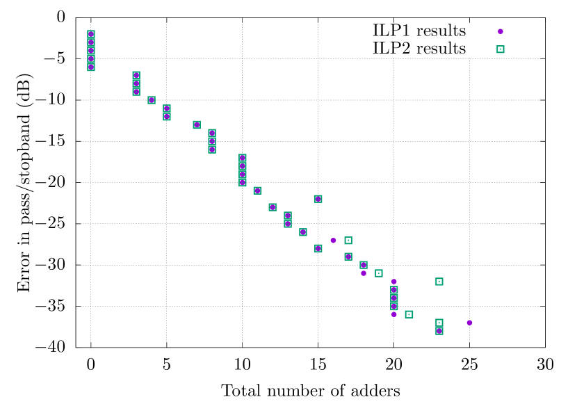
Figure 5: Total adder count comparison when using ILP1 (adapted to minimize the total number of adders) and ILP2 (with AD limit set to 2) on the Redmill set of filters [4].

For most error targets the resulting total adder count is identical between the two. The exceptions are $-27,-31,-32$ and $-36$ dB, where ILP1 gives a better total adder count, and $-37$ dB, where ILP2 is better. The four cases where ILP1 gives a better result are not surprising considering that the limited AD in ILP2 restricts the coefficient search space. For $-37$ dB, the difference comes from the fact that the ILP1 solver is able to find an optimal solution with $N=20$, while an $\text{AD}=2$ solution for ILP2 is only possible starting with $N=22$. Taking $\text{AD}=3$ with ILP2 gives the $N=20$ solution found with ILP1.

Due to the different nature of the constraints and objective values of both ILP models, it is hard to do a runtime comparison between the two. We only mention that when there is a feasible filter with small number of MB adders, ILP1 can be quite fast for moderate size problems ($N<50$), but turns out to struggle for problems with many MB adders. Similarly, for feasible designs with small AD (up to 3), ILP2 will be fast for $N<50$ and overall scales better than ILP1.

In the rest of the paper, for comparison with previous work, we use ILP Formulation 2 with $\text{AD}=2$ (unless otherwise stated).

VI-C2 Design Space Exploration for [4, Example 1]

The experiment setting from Section VI-C1 is expanded upon. We compare our best results (with effective word lengths $B\in\{8,9,10,11\}$) with those from [4, Example 1]. We start off by considering only type I filters (just like in [4]), variable gain $G\in[2/3,4/3]$ and minimal order $N$ for each error target. The results are illustrated in Figure 6. We note that there are certain cases where, for a given $B$, taking the minimal filter order leading to a feasible solution does not minimize the adder cost. This is most visible for $B=11$ and a $-30$dB error target, where a minimal order $N=14$ filter requires $24$ adders. For $B=10$, the minimal $N$ is $16$, leading to only $17$ total adders, a $7$ adder improvement. Taking $N=16$ for $B=11$ also results in a $17$ adder solution. A lower implementation cost is sometimes possible when increasing the filter order leads to a sparser filter and/or a more economical MCM design. Such solutions better optimize the objective functions in the proposed ILP models. We nevertheless remark that increasing the filter order beyond a certain threshold will not lead to different solutions [53].

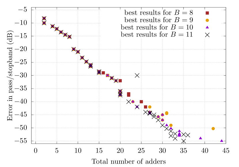
Figure 6: Our designs with effective word lengths varying from 8 to 11, filter type I and smallest feasible filter order.

Of course, increasing the word length can also lead to a significant improvement in the results. For instance, the optimal $-50$dB atteanuation results for $B\in\{9,10,11\}$ require $41,32$ and $31$ adders, respectively.

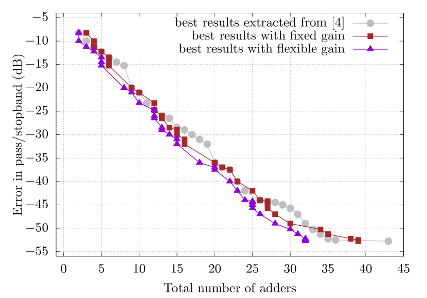
Figure 7: Comparison between our best design space exploration results and the best results from [4, Example 1]. Our tool improves designs from [4] or proves them optimal.

This nonlinearity of the word length/cost relation means that the user should favor a comprehensive exploration of the design space, varying the design parameters (especially $B$, filter type and $N$) and examine the various trade-offs. This is possible with our tool. Figure 7 shows the results of such an experiment where, with respect to the setting of Figure 6, we additionally allow $N$ to vary and also consider type II filters. We also added the flexible gain, genetic algorithm results produced in [4]. Compared to [4], we could improve all of the results, except two of them where we obtained the same adder cost ($-9$ dB and $-25$ dB). It is clearly visible that allowing variable gain designs can have a major influence on the quality of the results.

TABLE VI: Comparison between our method and the state-of-the-art results for the specifications in Table V.

Name	Source	$N$	Type	$A_{\text{M}}$	$A_{\text{S}}$	A	AD	$G$	$B$	Error	Coefficients
S1a	[2]	$24$	I	$11$	$24$	35	$2$	$2.41$	$8$	$0.00159$	$1$ $3$ $-1$ $-8$ $-7$ $10$ $20$ $-1$ $-40$ $-34$ $56$ $184$ $246$
S1a	ours	$24$	I	$7$	$20$	27	$2$	$1.251$	$9$	$\mathrm{𝟎}$	$1$ $4$ $\mathrm{𝟎}$ $-8$ $-7$ $10$ $22$ $\mathrm{𝟎}$ $-41$ $-36$ $57$ $192$ $256$
S1a	ours	$24$	I	$6$	$20$	26	$2$	$1.245678$	$9$	$0.00159$	$1$ $4$ $\mathrm{𝟎}$ $-8$ $-8$ $10$ $22$ $\mathrm{𝟎}$ $-40$ $-37$ $57$ $192$ $256$
S1a	ours	$23$	II	$7$	$19$	26	$2$	$2.654716$	$8$	$\mathrm{𝟎}$	$3$ $3$ $-5$ $-11$ $\mathrm{𝟎}$ $20$ $16$ $-23$ $-52$ $\mathrm{𝟎}$ $134$ $253$
S1a	ours	$23$	II	$5$	$19$	24	$2$	$2.172388$	$8$	$0.00159$	$2$ $2$ $-3$ $-9$ $\mathrm{𝟎}$ $16$ $13$ $-18$ $-42$ $\mathrm{𝟎}$ $110$ $208$
S1b	[4]	$24$	I	$6$	$20$	26	$3$	$2.4570$	$9$	$\mathrm{𝟎}$	$2$ $8$ $\mathrm{𝟎}$ $-16$ $-14$ $20$ $43$ $\mathrm{𝟎}$ $-80$ $-71$ $112$ $377$ $502$
S1b	ours	$24$	I	$6$	$20$	26	$2$	$1.40946$	$9$	$\mathrm{𝟎}$	$2$ $4$ $\mathrm{𝟎}$ $-10$ $-8$ $12$ $24$ $\mathrm{𝟎}$ $-47$ $-40$ $65$ $216$ $288$
S1b	ours	$23$	II	$5$	$19$	24	$2$	$2.46492$	$9$	$\mathrm{𝟎}$	$6$ $6$ $-8$ $-21$ $\mathrm{𝟎}$ $36$ $32$ $-42$ $-96$ $\mathrm{𝟎}$ $248$ $472$
S1b	ours	$23$	II	$7$	$19$	26	$2$	$2.65462$	$8$	$\mathrm{𝟎}$	$3$ $3$ $-5$ $-11$ $\mathrm{𝟎}$ $20$ $16$ $-23$ $-52$ $\mathrm{𝟎}$ $134$ $253$
S1c	[9]	$24$	I	$4$	$24$	28	$2$	$1.8950$	$8$	$\mathrm{𝟎}$	$2$ $3$ $-2$ $-8$ $-4$ $10$ $16$ $-3$ $-32$ $-24$ $48$ $144$ $191$
S1c	ours	$24$	I	$5$	$20$	25	$2$	$1.25615$	$8$	$\mathrm{𝟎}$	$1$ $2$ $\mathrm{𝟎}$ $-4$ $-3$ $6$ $11$ $\mathrm{𝟎}$ $-21$ $-18$ $29$ $96$ $128$
S1c	ours	$23$	II	$5$	$19$	24	$2$	$1.86904$	$7$	$\mathrm{𝟎}$	$1$ $1$ $-2$ $-4$ $\mathrm{𝟎}$ $7$ $6$ $-8$ $-18$ $\mathrm{𝟎}$ $47$ $89$
S1c	[13]	$23$	II	$4$	$19$	23	$2$	$1.34766$	$8$	$0.00118$	$2$ $2$ $-2$ $-5$ $\mathrm{𝟎}$ $10$ $8$ $-12$ $-26$ $\mathrm{𝟎}$ $68$ $128$
S1c	ours	$23$	II	$4$	$19$	23	$2$	$1.34717$	$8$	$0.00118$	$2$ $2$ $-2$ $-5$ $\mathrm{𝟎}$ $10$ $8$ $-12$ $-26$ $\mathrm{𝟎}$ $68$ $128$
S2a	[2]	$59$	II	$57$	$59$	116	$2$	$7.1324$	$13$	$\mathrm{𝟎}$	$31$ $28$ $29$ $22$ $8$ $-17$ $-59$ $-116$ $-188$ $-268$ $-352$ $-432$ $-500$ $-532$ $-529$ $-464$ $-336$ $-129$ $158$ $526$ $964$ $1472$ $2008$ $2576$ $3136$ $3648$ $4110$ $4478$ $4737$ $4868$
S2a	ours	$59$	II	$22$	$59$	81	$2$	$9.25424$	$10$	$\mathrm{𝟎}$	$4$ $4$ $4$ $4$ $1$ $-2$ $-9$ $-18$ $-30$ $-42$ $-56$ $-69$ $-80$ $-86$ $-85$ $-76$ $-56$ $-22$ $24$ $84$ $155$ $236$ $325$ $416$ $508$ $593$ $668$ $728$ $770$ $792$
S2b	[9]	$59$	II	$19$	$59$	78	$3$	$10.6888$	$10$	$\mathrm{𝟎}$	$5$ $5$ $6$ $5$ $3$ $-2$ $-10$ $-20$ $-32$ $-48$ $-64$ $-80$ $-91$ $-99$ $-99$ $-88$ $-64$ $-26$ $28$ $96$ $178$ $273$ $376$ $482$ $587$ $686$ $772$ $842$ $892$ $916$
S2b	[9]	$59$	II	$21$	$59$	80	$2$	$10.48712$	$10$	$\mathrm{𝟎}$	$5$ $5$ $5$ $4$ $2$ $-4$ $-10$ $-20$ $-34$ $-48$ $-64$ $-78$ $-91$ $-98$ $-96$ $-86$ $-62$ $-24$ $28$ $96$ $176$ $269$ $369$ $473$ $575$ $672$ $756$ $824$ $872$ $897$
S2b	ours	$59$	II	$19$	$57$	76	$2$	$10.506472$	$10$	$\mathrm{𝟎}$	$4$ $4$ $5$ $4$ $\mathrm{𝟎}$ $-4$ $-11$ $-22$ $-34$ $-49$ $-64$ $-79$ $-90$ $-98$ $-96$ $-84$ $-60$ $-24$ $30$ $97$ $178$ $270$ $370$ $474$ $576$ $672$ $756$ $824$ $872$ $896$
S2b	[13]	$59$	II	$17$	$59$	76	$3$	$10.47032$	$10$	$0.01395$	$5$ $5$ $6$ $5$ $2$ $-2$ $-10$ $-20$ $-32$ $-48$ $-64$ $-78$ $-92$ $-98$ $-87$ $-65$ $-26$ $26$ $93$ $174$ $267$ $368$ $472$ $575$ $672$ $757$ $826$ $874$ $898$
S2b	ours	$59$	II	$15$	$51$	66	$2$	$7.5904$	$10$	$0.00789$	$\mathrm{𝟎}$ $\mathrm{𝟎}$ $\mathrm{𝟎}$ $-2$ $-5$ $-10$ $-16$ $-23$ $-32$ $-40$ $-50$ $-58$ $-64$ $-64$ $-61$ $-50$ $-29$ $\mathrm{𝟎}$ $38$ $86$ $143$ $206$ $274$ $344$ $412$ $476$ $532$ $576$ $608$ $624$
L2	[9]	$62$	I	$17$	$62$	79	$3$	$2.6668$	$11$	$\mathrm{𝟎}$	$4$ $9$ $13$ $12$ $4$ $-10$ $-26$ $-36$ $-32$ $-12$ $18$ $44$ $52$ $32$ $-10$ $-56$ $-80$ $-64$ $-4$ $74$ $130$ $128$ $48$ $-86$ $-215$ $-263$ $-168$ $88$ $460$ $854$ $1153$ $1265$
L2	ours	$62$	I	$16$	$62$	78	$3$	$2.6668$	$11$	$\mathrm{𝟎}$	$4$ $9$ $13$ $12$ $4$ $-10$ $-26$ $-36$ $-32$ $-12$ $18$ $44$ $52$ $32$ $-10$ $-56$ $-80$ $-64$ $-4$ $74$ $130$ $128$ $48$ $-86$ $-215$ $-263$ $-168$ $88$ $460$ $854$ $1153$ $1265$
L3	[9]	$35$	II	$3$	$35$	38	$2$	$3.192$	$8$	$\mathrm{𝟎}$	$8$ $1$ $-6$ $-12$ $-10$ $-1$ $6$ $20$ $20$ $6$ $-12$ $-32$ $-40$ $-16$ $32$ $96$ $160$ $196$
L3	ours	$35$	II	$5$	$33$	38	$2$	$2.58268$	$7$	$\mathrm{𝟎}$	$4$ $\mathrm{𝟎}$ $-2$ $-4$ $-4$ $-1$ $4$ $7$ $8$ $3$ $-5$ $-14$ $-16$ $-7$ $12$ $39$ $64$ $79$
L3	ours	$35$	II	$5$	$31$	36	$1$	$2.6257$	$8$	$\mathrm{𝟎}$	$7$ $\mathrm{𝟎}$ $-5$ $-8$ $-10$ $\mathrm{𝟎}$ $6$ $15$ $15$ $8$ $-12$ $-28$ $-32$ $-14$ $24$ $80$ $130$ $160$
L3	ours	$35$	II	$4$	$31$	35	$2$	$2.10468$	$8$	$\mathrm{𝟎}$	$5$ $\mathrm{𝟎}$ $-4$ $-8$ $-8$ $\mathrm{𝟎}$ $4$ $11$ $13$ $5$ $-10$ $-22$ $-26$ $-11$ $20$ $64$ $104$ $129$
L3	[13]	$35$	II	$4$	$31$	35	$1$	$2.627$	$7$	$0.00213$	$3$ $\mathrm{𝟎}$ $-2$ $-5$ $-5$ $\mathrm{𝟎}$ $3$ $7$ $8$ $3$ $-6$ $-14$ $-16$ $-7$ $12$ $40$ $65$ $80$
L3	ours	$35$	II	$4$	$31$	35	$1$	$2.61998$	$7$	$0.00213$	$3$ $\mathrm{𝟎}$ $-2$ $-4$ $-6$ $\mathrm{𝟎}$ $3$ $7$ $7$ $4$ $-6$ $-14$ $-16$ $-7$ $12$ $40$ $65$ $80$
L3	ours	$35$	II	$5$	$29$	34	$2$	$2.6211$	$8$	$0.00213$	$7$ $\mathrm{𝟎}$ $\mathrm{𝟎}$ $-10$ $-8$ $\mathrm{𝟎}$ $8$ $16$ $16$ $7$ $-10$ $-28$ $-32$ $-14$ $24$ $78$ $130$ $160$
L3	ours	$35$	II	$3$	$31$	34	$1$	$2.60028$	$8$	$0.00213$	$6$ $\mathrm{𝟎}$ $-3$ $-10$ $-10$ $\mathrm{𝟎}$ $7$ $12$ $16$ $7$ $-12$ $-28$ $-32$ $-14$ $24$ $80$ $128$ $160$
L3	ours	$35$	II	$3$	$31$	34	$2$	$2.60564$	$7$	$0.00213$	$4$ $\mathrm{𝟎}$ $-2$ $-4$ $-4$ $\mathrm{𝟎}$ $3$ $8$ $8$ $3$ $-6$ $-13$ $-16$ $-8$ $13$ $40$ $64$ $80$

VI-C3 The Set of State-of-the-art Specifications

Table VI-C2 presents the comparison between our designs and the best results from literature [1, 2, 4, 9, 12, 13, 15] for the filter specifications from Table V. The following information for each implementation is given: filter order ($N$), filter type, number of multiplier adders ($A_{M}$), number of structural adders ($A_{S}$), total number of adders ($A$), adder depth of the multiplier block (AD), gain ($G$), effective coefficient word length ($B$), frequency response error and, finally, coefficients of the filter. The frequency response error represents by how much the resulting filter does not respect the specification (zero in case of no issue) and was necessary to introduce since coefficients from previous work turned out to sometimes slightly violate the specification. For those cases we also adjusted the specification to find solutions with a similar error in order to perform a fair and complete comparison. In the following, we discuss each instance in detail.

S1a

we obtain a 23% improvement (27 vs. 35 adders) in comparison to the implementation in [2]. By also considering type II designs, one extra adder can be saved (26 total adders). If furthermore a slight error is allowed, a design with 24 adders is achievable.

S1b

for this specification we show that, for type I designs, the AD can be reduced from 3 to 2 stages, while keeping the same effective word length. If we use type II filters, keeping the same word length as [4] allows the reduction of two adders (one structural and one MB). We can also decrease the word length by one, and still get a result with the same cost as [4].

S1c

we improve the result from [9] by 3 adders by prioritizing sparse implementations. For type II specifications we can gain one extra structural adder and decrease the word length by one. A type II implementation of these specifications from [13] requires only 23 adders but has higher error than that allowed by the specification. If we allow some error, we obtain the same 23 adder solution as [13].

S2a

we offer a significant improvement in the implementation of this specification w.r.t. the best known result [2]. Our solution requires 30% less adders (81 adders vs. 116 adders) and we reduce the effective word length from 13 to 10 bits.

S2b

in [9], implementations with adder depths 3 and 2 are proposed, at the cost of 78 and 80 adders, respectively. These results are improved in [13], with the authors claiming that a 3-stage implementation at the cost of 76 adders has a high probability to be optimal. Our check shows that the latter design does not pass an a posteriori validation by a margin of at least $0.01395$. If some error margin is indeed acceptable, we demonstrate that a 2-stage design with a cost of only 66 adders is possible. Again, our result has higher sparsity than previous designs. If frequency specifications must be rigorously met, we show that 76 adders is the optimal cost for a 2-stage design.

L1

the tool timed out for this specification before giving a feasible result, hence it is not presented in Table VI-C2. The best known result from literature is a 120-tap filter [9] and the size of an instance of the corresponding ILP formulation goes beyond the current capabilities of the solvers we tried, showing its limitations.

L2

the result of [9] can be improved by one adder with the same coefficient set. Similar to L1, we had to timeout before the solver could ascertain if the feasible filter obtained is indeed optimal.

L3

in [9], an implementation with 38 adders is provided. As in the case of the S2b specification, [13] reduces both the adder count and adder depth, but at the cost of a substantial violation of the frequency specifications. We improve on the result from [9], proving that only a 7-bit wordlength is necessary to get the same 38 adder cost. This cost can be reduced to 35 adders by using 8-bit coefficients. If we allow the same error as in [13], we show that 34 adder solutions are possible.

Overall, the proposed tool achieves significant improvements to the majority of the considered filter design problems. Morover, the user can explore a large design space by setting different implementation parameters, e.g. adder depth, coefficient word length, filter type, etc. The required runtime however, will depend greatly on the problem. For producing the results in Table VI-C2, it varied from several seconds for the smallest filters (S1) up to several days for the largest ones (S2 and L2).

VII Conclusion

In this paper we have introduced two new algorithms for the design of optimal multiplierless FIR filters. Relying on ILP formulations stemming from the MCM literature, our algorithms minimize either (a) the number of structural adders given a fixed budget of multiplier block adders or (b) the total number of adders (multiplier block + structural adders) given a fixed adder depth. We further show how (a) can be applied iteratively to optimally minimize the total number of adders (without any adder count or adder depth constraints). Extensive numerical tests with example design problems from the state-of-the-art show that our approaches can offer in many cases better results. We also make available an open-source C++ implementation of the proposed methods.

References

- [1] Y. Lim and S. Parker, “FIR filter design over a discrete powers-of-two coefficient space,” IEEE Transactions on Acoustics, Speech, and Signal Processing, vol. 31, no. 3, pp. 583–591, 1983.
- [2] H. Samueli, “An improved search algorithm for the design of multiplierless FIR filters with powers-of-two coefficients,” IEEE Transactions on Circuits and Systems, vol. 36, no. 7, pp. 1044–1047, Jul. 1989.
- [3] R. I. Hartley, “Subexpression sharing in filters using canonic signed digit multipliers,” IEEE Transactions on Circuits and Systems II: Analog and Digital Signal Processing, vol. 43, no. 10, pp. 677–688, 1996.
- [4] D. Redmill, D. Bull, and E. Dagless, “Genetic synthesis of reduced complexity filters and filter banks using primitive operator directed graphs,” Circuits, Devices and Systems, IEE Proceedings -, vol. 147, no. 5, pp. 303–310, 2000.
- [5] O. Gustafsson and H. Johansson, “An MILP approach for the design of linear-phase FIR filters with minimum number of signed-power-of-two terms,” es.isy.liu.se, 2001.
- [6] J. Yli-Kaakinen and T. Saramaki, “A systematic algorithm for the design of multiplierless FIR filters,” IEEE International Symposium on Circuits and Systems, vol. 2, pp. 185–188, 2001.
- [7] O. Gustafsson and L. Wanhammar, “Design of linear-phase FIR filters combining subexpression sharing with MILP,” in Midwest Symposium on Circuits and Systems. IEEE, Aug. 2002, pp. III–9–III–12.
- [8] A. P. Vinod and E.-K. Lai, “On the implementation of efficient channel filters for wideband receivers by optimizing common subexpression elimination methods,” IEEE Transactions on Computer-Aided Design of Integrated Circuits and Systems, vol. 24, no. 2, pp. 295–304, 2005.
- [9] Y. J. Yu and Y. C. Lim, “Design of Linear Phase FIR Filters in Subexpression Space Using Mixed Integer Linear Programming,” IEEE Transactions on Circuits and Systems I: Regular Papers, vol. 54, no. 10, pp. 2330–2338, 2007.
- [10] M. Aktan, A. Yurdakul, and G. Dundar, “An algorithm for the design of low-power hardware-efficient FIR filters,” IEEE Transactions on Circuits and Systems I: Regular Papers, vol. 55, no. 6, pp. 1536–1545, 2008.
- [11] Y. Yu and Y. Lim, “Optimization of Linear Phase FIR Filters in Dynamically Expanding Subexpression Space,” Circuits, Systems, and Signal Processing, vol. 29, no. 1, pp. 1–16, 2009.
- [12] Y. J. Yu, D. Shi, and Y. C. Lim, “Design of extrapolated impulse response FIR filters with residual compensation in subexpression space,” IEEE Transactions on Circuits and Systems I: Regular Papers, 2009.
- [13] D. Shi and Y. J. Yu, “Design of Linear Phase FIR Filters With High Probability of Achieving Minimum Number of Adders,” IEEE Transactions on Circuits and Systems I: Regular Papers, vol. 58, no. 1, pp. 126–136, 2011.
- [14] ——, “Design of Discrete-Valued Linear Phase FIR Filters in Cascade Form,” IEEE Transactions on Circuits and Systems I: Regular Papers, vol. 58, no. 7, pp. 1627–1636, 2011.
- [15] A. Shahein, Q. Zhang, N. Lotze, and Y. Manoli, “A Novel Hybrid Monotonic Local Search Algorithm for FIR Filter Coefficients Optimization,” IEEE Transactions on Circuits and Systems I: Regular Papers, vol. 59, no. 3, pp. 616–627, 2012.
- [16] W. Bin Ye and Y. J. Yu, “A polynomial-time algorithm for the design of multiplierless linear-phase FIR filters with low hardware cost,” IEEE International Symposium on Circuits and Systems (ISCAS), pp. 970–973, 2014.
- [17] W. B. Ye and Y. J. Yu, “Bit-level multiplierless FIR filter optimization incorporating sparse filter technique,” IEEE Transactions on Circuits and Systems I: Regular Papers, vol. 61, no. 11, pp. 3206–3215, 2014.
- [18] A. Mehrnia and A. N. Willson, “Optimal Factoring of FIR Filters,” IEEE Transactions on Signal Processing, vol. 63, no. 3, pp. 647–661, Feb. 2015.
- [19] W. B. Ye, X. Lou, and Y. J. Yu, “Design of Low Power Multiplierless Linear-Phase FIR Filters,” IEEE Access, 2017.
- [20] X. Lou, P. K. Meher, Y. Yu, and W. Ye, “Novel Structure for Area-Efficient Implementation of FIR Filters,” IEEE Transactions on Circuits and Systems II: Express Briefs, vol. 64, no. 10, pp. 1212–1216, 2017.
- [21] P. Cappello and K. Steiglitz, “Some Complexity Issues in Digital Signal Processing,” IEEE Transactions on Acoustics, Speech and Signal Processing, vol. 32, no. 5, pp. 1037–1041, Oct. 1984.
- [22] A. Dempster and M. Macleod, “Use of Minimum-Adder Multiplier Blocks in FIR Digital Filters,” IEEE Transactions on Circuits and Systems II: Analog and Digital Signal Processing, vol. 42, no. 9, pp. 569–577, 1995.
- [23] Y. Voronenko and M. Püschel, “Multiplierless Multiple Constant Multiplication,” ACM Transactions on Algorithms, vol. 3, no. 2, pp. 1–38, 2007.
- [24] O. Gustafsson, “A Difference Based Adder Graph Heuristic for Multiple Constant Multiplication Problems,” in IEEE International Symposium on Circuits and Systems (ISCAS), 2007, pp. 1097–1100.
- [25] ——, “Towards Optimal Multiple Constant Multiplication: A Hypergraph Approach,” in Asilomar Conference on Signals, Systems and Computers (ACSSC). IEEE, Oct. 2008, pp. 1805–1809.
- [26] L. Aksoy, E. Günes, and P. Flores, “Search Algorithms for the Multiple Constant Multiplications Problem: Exact and Approximate,” Microprocessors and Microsystems, vol. 34, no. 5, pp. 151–162, 2010.
- [27] M. Kumm, “Optimal Constant Multiplication using Integer Linear Programming,” IEEE Transactions on Circuits and Systems II: Express Briefs, 2018.
- [28] R. E. Crochiere and A. V. Oppenheim, “Analysis of Linear Digital Networks,” in Proceedings of the IEEE, 1975, pp. 581–595.
- [29] D. M. Kodek, “Design of optimal finite wordlength FIR digital filters using integer programming techniques,” IEEE Transactions on Acoustics, Speech and Signal Processing, vol. 28, no. 3, pp. 304–308, 1980.
- [30] J. M. de Sa, “A new design method of optimal finite wordlength linear phase FIR digital filters,” IEEE Transactions on Acoustics, Speech, and Signal Processing, vol. 31, no. 4, pp. 1032–1034, 1983.
- [31] Y. Lim, “Design of discrete-coefficient-value linear phase FIR filters with optimum normalized peak ripple magnitude,” IEEE Transactions on Circuits and Systems, vol. 37, no. 12, pp. 1480–1486, 1990.
- [32] D. M. Kodek, “Design of optimal finite wordlength FIR digital filters,” in Proc. of the European Conference on Circuit Theory and Design, ECCTD ’99., vol. 1, Aug. 1999, pp. 401–404.
- [33] ——, “Performance limit of finite wordlength FIR digital filters,” IEEE Transactions on Signal Processing, vol. 53, no. 7, pp. 2462–2469, 2005.
- [34] ——, “LLL algorithm and the optimal finite wordlength FIR design,” IEEE Transactions on Signal Processing, vol. 60, no. 3, pp. 1493–1498, 2012.
- [35] A. Antoniou, Digital Signal Processing: Signals, Systems, and Filters. McGraw-Hill Education, 2005.
- [36] M. Faust and C.-H. Chang, “Minimal Logic Depth Adder Tree Optimization for Multiple Constant Multiplication,” IEEE International Symposium on Circuits and Systems (ISCAS), pp. 457–460, 2010.
- [37] S. Demirsoy, A. Dempster, and I. Kale, “Transition Analysis on FPGA for Multiplier-Block Based FIR Filter Structures,” IEEE International Symposium of Circuits and Systems (ISCAS), vol. 2, pp. 862–865 vol.2, 2000.
- [38] ——, “Power Analysis of Multiplier Blocks,” in IEEE International Symposium on Circuits and Systems (ISCAS), 2002, pp. I–297–I–300 vol.1.
- [39] A. G. Dempster, S. S. Demirsoy, and I. Kale, “Designing Multiplier Blocks with Low Logic Depth,” in IEEE International Symposium on Circuits and Systems (ISCAS). IEEE, 2002, pp. V–773–V–776.
- [40] M. Kumm, “Multiple Constant Multiplication Optimizations for Field Programmable Gate Arrays,” Ph.D. dissertation, Springer Wiesbaden, Wiesbaden, Oct. 2015.
- [41] A. Dempster and M. D. Macleod, “Constant Integer Multiplication Using Minimum Adders,” IEE Proceedings of Circuits, Devices and Systems, vol. 141, no. 5, pp. 407–413, 1994.
- [42] M. Kumm, D. Fanghänel, K. Möller, P. Zipf, and U. Meyer-Baese, “FIR Filter Optimization for Video Processing on FPGAs,” Springer EURASIP Journal on Advances in Signal Processing, pp. 1–18, 2013.
- [43] H.-J. Kang and I.-C. Park, “FIR Filter Synthesis Algorithms for Minimizing the Delay and the Number of Adders,” IEEE Transactions on Circuits and Systems II: Analog and Digital Signal Processing, vol. 48, no. 8, pp. 770–777, 2001.
- [44] D. Chan and L. Rabiner, “Analysis of Quantization Errors in the Direct Form for Finite Impulse Response Digital Filters,” IEEE Transactions on Audio and Electroacoustics, vol. 21, no. 4, pp. 354–366, Aug. 1973.
- [45] A. Volkova, C. Lauter, and T. Hilaire, “Reliable verification of digital implemented filters against frequency specifications,” in 2017 IEEE 24th Symposium on Computer Arithmetic (ARITH), July 2017, pp. 180–187.
- [46] S.-I. Filip, “A robust and scalable implementation of the Parks-McClellan algorithm for designing FIR filters,” ACM Transactions on Mathematical Software (TOMS), vol. 43, no. 1, p. 7, 2016.
- [47] N. Brisebarre, S.-I. Filip, and G. Hanrot, “A Lattice Basis Reduction Approach for the Design of Finite Wordlength FIR Filters,” IEEE Transactions on Signal Processing, vol. 66, no. 10, pp. 2673–2684, May 2018.
- [48] A. V. Oppenheim and R. W. Schafer, Discrete-time signal processing. Pearson Education, 2014.
- [49] A. Gleixner et al., “The SCIP Optimization Suite 6.0,” http://www.optimization-online.org/DB_HTML/2018/07/6692.html, Optimization Online, Technical Report, July 2018.
- [50] “Gurobi optimization system,” https://www.gurobi.com.
- [51] “CPLEX optimizer,” https://www.ibm.com/analytics/cplex-optimizer.
- [52] P. Sittel, T. Schönwälder, M. Kumm, and P. Zipf, “ScaLP: A Light-Weighted (MI)LP Library,” in Methoden und Beschreibungssprachen zur Modellierung und Verifikation von Schaltungen und Systemen (MBMV), 2018, pp. 1–10.
- [53] D. M. Kodek, “Length limit of optimal finite wordlength FIR filters,” Digital Signal Processing, vol. 23, no. 5, pp. 1798–1805, Sep. 2013.