Solving Bayesian Inverse Problems via Variational Autoencoders

Abstract

In recent years, the field of machine learning has made phenomenal progress in the pursuit of simulating real-world data generation processes. One notable example of such success is the variational autoencoder (VAE). In this work, with a small shift in perspective, we leverage and adapt VAEs for a different purpose: uncertainty quantification (UQ) in scientific inverse problems. We introduce UQ-VAE: a flexible, adaptive, hybrid data/model-constrained framework for training neural networks capable of rapid modelling of the posterior distribution representing the unknown parameter of interest. Specifically, from divergence-based variational inference, our framework is derived such that most of the information usually present in scientific inverse problems is fully utilized in the training procedure. Additionally, this framework includes an adjustable hyperparameter that allows selection of the notion of distance between the posterior model and the target distribution. This introduces more flexibility in controlling how optimization directs the learning of the posterior model. Further, this framework possesses an inherent adaptive optimization property that emerges through the learning of the posterior uncertainty. Numerical results for an elliptic PDE-constrained Bayesian inverse problem are provided to verify the proposed framework.

1 Introduction

The challenge of generative modelling is often approached through optimization of a parameterized likelihood function $p_{\boldsymbol{\theta}}(\textbf{x})$ to learn the optimal parameters $\boldsymbol{\theta}$. Latent variable models augment this likelihood function using an unobservable latent variable in hopes that one can also learn useful latent representations that facilitate reconstruction and generation of high-dimensional distributions. Variational autoencoders (VAE) were introduced in [Kingma and Welling(2013)] to train a generating function that maps from the latent space to the target data distribution. The approach in [Kingma and Welling(2013)] assumes the latent distribution to simply be an isotropic Gaussian $p\left(\textbf{z}\right)=\mathcal{N}\left(\textbf{z}|\boldsymbol{0},\boldsymbol{I}\right)$; thereby shifting all the burden of generative modelling to the learning of the generating function. To address the infeasibly large number of draws from the isotropic Gaussian required to ensure significant contribution to the likelihood function, [Kingma and Welling(2013)] proposes to instead draw from the posterior distribution $p_{\boldsymbol{\theta}}(\textbf{z}|\textbf{x})$. This introduces the subtask of variational inference; the modelling of the posterior with a distribution $q_{\boldsymbol{\phi}}(\textbf{z}|\textbf{x})$ parameterized by an additional set of learnable parameters $\boldsymbol{\phi}$. The learning of the parameters $\boldsymbol{\phi}$ can be achieved through the minimization of the Evidence Lower Bound (ELBO) [Blei et al.(2017)Blei, Kucukelbir, and McAuliffe]; a quantity obtainable through the Kullback-Leibler divergence (KLD) between the model posterior and the target posterior.

Although the goal of generative modelling fundamentally differs from that of scientific inverse problems, we claim that VAEs are also well suited for the latter challenge. In the setting of physical systems, scientific inverse problems task us with determining parameters-of-interest (PoI) given observations of a state variable. Often, these parameters are coefficients in a partial differential equation (PDE) governing the system and the observations are discrete measurements of the state variables of the PDE. Assuming that our observations are corrupted by additive noise, then the equation

$$\textbf{y}_{\mathrm{obs}}=\mathcal{F}(\textbf{u})+\textbf{e}$$ (1)

represents the connection between the PoI and observational data. Here, u denotes a discretized representation of the PoI, $\mathcal{F}$ denotes the parameter-to-observable (PtO) map and $\textbf{y}_{\mathrm{obs}}$ denotes our observational data.

To bridge the two contexts, we consider the latent space and generating function in latent variable models to be the PoI space and the PtO map in inverse problems. Therefore, while the former uses inference to facilitate generative modelling, the latter uses generative modelling to facilitate inference. We contrast the two settings under this viewpoint in order to expose the utility of VAEs for scientific inverse problems:

1. For generative modelling, the focus of training VAEs is to learn the generating function. In contrast, for scientific inverse problems, the PtO map need not be learnt as it can often be modelled using physics-based numerical methods.

2. For generative modelling, the latent space of VAEs is an unspecified quantity with properties emerging almost entirely though the process of learning the generating function. In contrast, for scientific inverse problems, by considering the latent space to be the PoI space, the latent space therefore possesses structure that represents the physical properties of the PoI.

Therefore, the context of scientific inverse problems provides more information that can be exploited to improve the training procedure of a VAE. Indeed, in reference to the first point, one can surrogate the generating function with a physics-based numerical model of the PtO map. In doing so, the focus of the training is shifted completely towards inference. In reference to the second point, knowledge of the physical properties of the PoI can be encoded in the prior model which, therefore, allows for a more informative latent distribution than the isotropic Gaussian used in [Kingma and Welling(2013)]. Further, through scientific experimentation or simulation, one may have on hand a dataset of PoI and observation pairs $\left\{\left(\textbf{u}^{(m)},\textbf{y}_{\mathrm{obs}}^{(m)}\right)\right\}_{m=1}^{M}$. To draw an analogy within the context of generative modelling, the datapoints $\textbf{u}^{(m)}$ are analogous to latent data that is usually not available. This advantage provides the main motivation for our proposed UQ-VAE framework: a mathematically justified training procedure for a VAE that can utilize the latent data we possess.

2 Preliminaries and Motivation

In scientific inverse problems, the solution process for obtaining estimates of the PoI often involves the optimization of a functional of the form

$$\min_{\textbf{u}}\left\lVert\textbf{y}_{\mathrm{obs}}-\mathcal{F}(\textbf{u})\right\rVert_{2}^{2}.$$ (2)

Whilst the observations are finite-dimensional entities, the PoI often exists in an infinite-dimensional function space. Thus, our task is complicated by the inherent ill-posed nature of inverse problems; there are many possible estimates of the PoI that are consistent with the observations. To alleviate this issue, regularization can be introduced to essentially reduce the size of the solution space. With the introduction of a regularization term, the optimization problem (2) becomes

$$\min_{\textbf{u}}\left\lVert\textbf{y}_{\mathrm{obs}}-\mathcal{F}(\textbf{u})\right\rVert_{2}^{2}+\mathcal{R}(\textbf{u}).$$ (3)

The optimization of (3) is often a time-consuming process; for example when using derivative-based iterative optimization algorithms. This motivates the need for an inverse problems solver that can rapidly output PoI estimates from given observational data.

2.1 Learning a Solver for Deterministic Inverse Problems

We briefly discuss data-driven deterministic inverse problem solvers to motivate both the concept of UQ as well as our proposed training procedure.

Suppose that we are tasked with learning an inverse problem solver using a training dataset of $M$ PoI and observation pairs $\left\{\left(\textbf{u}^{(m)},\textbf{y}_{\mathrm{obs}}^{(m)}\right)\right\}_{m=1}^{M}$. If we elect to use a neural network $\Psi$, then our solver is parameterized by the weights $\boldsymbol{W}$ of the network. Analogous to (3), the training of this solver requires the optimization of the following functional:

$$\min_{\boldsymbol{W}}\frac{1}{M}\sum_{m=1}^{M}\left\lVert\textbf{u}^{(m)}-\Psi\left(\textbf{y}_{\mathrm{obs}}^{(m)},\boldsymbol{W}\right)\right\rVert_{2}^{2}+\mathcal{R}(\boldsymbol{W}).$$ (4)

Following the offline training stage of the neural network, we obtain a rapid online inverse problem solver that can output an estimate of our PoI given observation data. However, the ill-posed nature of inverse problems is inherited by this task; there are many possible weights that can be used to parameterize a solver that outputs PoI estimates consistent with the input observational data. Further, while the regularization term in (3) can be designed based on some prior knowledge of the physical properties of the PoI, the physical interpretation of the neural network weights is not so clear. Therefore, there is no natural choice for the regularization of the optimization problem (4).

Instead of regularizing the weights of the network directly, one possible approach is to regularize the output of the network. For example, we could make use of the PtO map so that (4) becomes

$$\min_{\boldsymbol{W}}\frac{1}{M}\sum_{m=1}^{M}\left\lVert\textbf{u}^{(m)}-\Psi\left(\textbf{y}_{\mathrm{obs}}^{(m)},\boldsymbol{W}\right)\right\rVert_{2}^{2}+\left\lVert\textbf{y}_{\mathrm{obs}}^{(m)}-\mathcal{F}\left(\Psi\left(\textbf{y}_{\mathrm{obs}}^{(m)},\boldsymbol{W}\right)\right)\right\rVert_{2}^{2}.$$ (5)

In doing so, the PtO map indirectly informs the weights of the neural network of the inversion task. An additional benefit with the inclusion of the PtO map is that we are also able to include noise regularization. That is, if we possess some knowledge about the properties of the noise e afflicting our observational data, we may quantify it and include it in the second term to yield

$$\min_{\boldsymbol{W}}\frac{1}{M}\sum_{m=1}^{M}\left\lVert\textbf{u}^{(m)}-\Psi\left(\textbf{y}_{\mathrm{obs}}^{(m)},\boldsymbol{W}\right)\right\rVert_{2}^{2}+\left\lVert\mathcal{M}\left(\textbf{y}_{\mathrm{obs}}^{(m)}-\mathcal{F}\left(\Psi\left(\textbf{y}_{\mathrm{obs}}^{(m)},\boldsymbol{W}\right)\right)\right)\right\rVert_{2}^{2}$$ (6)

where $\mathcal{M}$ represents some noise regularization mapping. Furthermore, if we possess some prior knowledge about the physical properties of the parameter of interest, we may also include it as follows:

$$\min_{\boldsymbol{W}}\frac{1}{M}\sum_{m=1}^{M}\left\lVert\textbf{u}^{(m)}-\Psi\left(\textbf{y}_{\mathrm{obs}}^{(m)},\boldsymbol{W}\right)\right\rVert_{2}^{2} +\left\lVert\mathcal{M}\left(\textbf{y}_{\mathrm{obs}}^{(m)}-\mathcal{F}\left(\Psi\left(\textbf{y}_{\mathrm{obs}}^{(m)},\boldsymbol{W}\right)\right)\right)\right\rVert_{2}^{2}$$ (7a)

$$+\left\lVert\mathcal{P}\left(\Psi\left(\textbf{y}_{\mathrm{obs}}^{(m)},\boldsymbol{W}\right)\right)\right\rVert_{2}^{2}$$ (7b)

where $\mathcal{P}$ is some prior regularization mapping.

Training a neural network through the optimization problem (7) yields a learned inverse problems solver that outputs a point estimate of our PoI. As it is, this deterministic solver is unable to provide information about the accuracy of the estimate. It would be more ideal to have a probabilistic interpretation of our learned solver that facilitates UQ. With this in mind, we are motivated to view inverse problems under the framework of Bayesian statisics. In this setting, we instead work towards a solver for Bayesian inverse problems which, in turn, allows us to formally establish the regularization terms in (7). Conversely, by ignoring the uncertainty estimate, the UQ-VAE solver recovers the deterministic setting (7).

2.2 Learning a Solver for Bayesian Inverse Problems

Under the statistical framework, the PoI of an inverse problem is considered to be a random variable instead of an unknown value. Consequently, the solution of the statistical inverse problem is a probability distribution instead of a single estimated value. By adopting a statistical framework instead of deterministic, the question asked by the inverse problem essentially changes from “what is the value of our parameter?” to “how accurate is the estimate of our parameter?”. Further, the statistical framework attempts to remove the ill-posedness of inverse problems by restating the inverse problem as a well-posed extension in a larger space of probability distributions [Kaipio and Somersalo(2006), Dashti and Stuart(2013)].

With an additive noise assumption, we consider the following observational model

$$Y=\mathcal{F}\left(U\right)+E$$ (8)

where $\mathcal{F}$ is the PtO map and $Y$, $U$ and $E$ are the random variables representing the observational data, PoI and noise model respectively. Since $U$ is unknown to us, we represent its uncertainty with a probability distribution constructed from prior knowledge. However, we do not use equation (8) directly when working under a statistical framework. Instead, we primarily consider the relations between the probability distributions of the random variables involved to answer the question: “given the observational data $\textbf{y}_{\mathrm{obs}}$, what is the distribution of the PoI $U$ responsible for our measurement?”. Therefore, the conditional density $p_{U|Y}\left(\textbf{u}|Y=\textbf{y}_{\mathrm{obs}}\right)$ is the solution to the statistical parameter estimation problem under the Bayesian framework. To approximate this conditional density, we utilize Bayes’ Theorem to form a model of $p_{U|Y}\left(\textbf{u}|Y=\textbf{y}_{\mathrm{obs}}\right)$ called the posterior distribution which we denote as $p_{\mathrm{post}}$:

$$p_{\mathrm{post}}\left(\textbf{u}|\textbf{y}_{\mathrm{obs}}\right)\propto p_{\mathrm{lkhd}}\left(\textbf{y}_{\mathrm{obs}}|\textbf{u}\right)p_{\mathrm{pr}}\left(\textbf{u}\right).$$ (9)

where $p_{\mathrm{lkhd}}$ is the likelihood model and $p_{\mathrm{pr}}$ is the prior model.

Formulating the parameter estimation problem under a Bayesian framework requires us to obtain (9). This challenges us with the completion of three tasks:

1. construct the likelihood model $p_{\mathrm{lkhd}}$ that expresses the interrelation between the data and the unknown,

2. using prior information we may possess about the unknown u, construct a prior probability density $p_{\mathrm{pr}}$ that expresses this information,

3. develop methods which extract meaningful information from the posterior density $p_{\mathrm{post}}$.

To address these three tasks, two assumptions are often made. The first assumption supposes that the noise $E$ is mutually independent with respect to the PoI $U$. Then, using our observation model (8) and marginalization of the noise $E$, we obtain the following likelihood model:

$$p_{\mathrm{lkhd}}=p_{E}\left(\textbf{y}_{\mathrm{obs}}-\mathcal{F}\left(\textbf{u}\right)\right).$$ (10)

The second assumption supposes that all are random variables are Gaussian with $\mathcal{N}(\boldsymbol{\mu}_{E},\boldsymbol{\Gamma}_{E})$ and $\mathcal{N}(\boldsymbol{\mu}_{\mathrm{pr}},\boldsymbol{\Gamma}_{\mathrm{pr}})$. With this, our posterior model becomes

$$p_{\mathrm{post}}(\textbf{u}|\textbf{y}_{\mathrm{obs}}) \propto p_{E}(\textbf{y}_{\mathrm{obs}}-\mathcal{F}(\textbf{u}))p_{\mathrm{pr}}(\textbf{u})$$ (11a)

$$=\exp{\left(-\frac{1}{2}\left(\left\lVert\textbf{y}_{\mathrm{obs}}-\mathcal{F}(\textbf{u})-\boldsymbol{\mu}_{E}\right\rVert_{\boldsymbol{\Gamma}_{E}^{-1}}^{2}+\left\lVert\textbf{u}-\boldsymbol{\mu}_{\mathrm{pr}}\right\rVert_{\boldsymbol{\Gamma}_{\mathrm{pr}}^{-1}}^{2}\right)\right)}.$$ (11b)

In order to perform UQ with given observational data $\textbf{y}_{\mathrm{obs}}$, one often seeks an approximation of the posterior covariance of (11). A commonly used approximation is the Laplace approximation [Evans and Swartz(2000), Press(2009), Stigler(1986), Tierney and Kadane(1986), Wong(2001)]

$$\boldsymbol{\Gamma}_{\mathrm{post}}=\left(\boldsymbol{J}_{\mathcal{F}}(\textbf{u}_{\mathrm{map}})^{\mathrm{T}}\boldsymbol{\Gamma}_{E}^{-1}\boldsymbol{J}_{\mathcal{F}}(\textbf{u}_{\mathrm{map}})+\boldsymbol{\Gamma}_{\mathrm{pr}}^{-1}\right)^{-1}$$ (12)

where $\textbf{u}_{\mathrm{map}}$ is the maximum a posteriori (MAP) estimate and $\boldsymbol{J}_{\mathcal{F}}(\textbf{u}_{\mathrm{map}})$ is the Jacobian of $\mathcal{F}$ at the MAP estimate. The MAP estimate can be obtained through optimization of the exponentiated functional in (11b); which often requires a potentially expensive derivative-based iterative optimization procedure. Markov Chain Monte Carlo (MCMC) methods can also be employed but such methods notably suffer the curse of dimensionality.

This desire for efficient UQ also motivates our work. Although the training procedure of a Bayesian inverse problems solver may be computationally demanding, it represents an offline stage. Once trained, the online stage of UQ has a computational cost governed only by the forward propagation of the observational data through the trained neural network; which is often a very computationally efficient procedure.

Additionally, the PoI data $\textbf{u}^{(m)}$ in the training dataset $\left\{\left(\textbf{u}^{(m)},\textbf{y}_{\mathrm{obs}}^{(m)}\right)\right\}_{m=1}^{M}$ usually plays no role in traditional methods. Information about the PoI is often only encoded in the prior model. This motivates the data-driven aspect of our approach in that we not only use prior information but we also take advantage of PoI data in the cases where paired PoI-observation datasets are readily obtainable.

With this motivation in mind, we now detail a proposed framework for training our solver. When comparing with (7) from Section 2.1, the exponentiated functional in (11b) looks like an appealing candidate for the regularization terms. We formalize the inclusion of these terms as regularizers through the derivation of our proposed framework for data-driven UQ.

3 Flexible, Adaptive, Hybrid Data/Model-Constrained Framework for UQ

We begin by detailing the derivation of our proposed UQ-VAE framework before discussing from the more tractable perspective of optimization. While the former centers the discussion more in the setting of variational inference, the latter is centered more towards regularization of the training procedure for our solver. Further, whilst the flexibility of our framework emerges through the viewpoint of variational inference, the optimization viewpoint uncovers its inherent adaptive properties.

3.1 Derivation of the UQ-VAE Framework

Let $p(\textbf{u}|\textbf{y})$ denote the target posterior density we wish to estimate and let $q_{\boldsymbol{\phi}}(\textbf{u}|\textbf{y})$ denote our model of the target density with statistics parameterized by $\boldsymbol{\phi}$. To optimize for the parameters $\boldsymbol{\phi}$, we require some notion of distance between our model posterior and target posterior. In this work, instead of using the KLD to obtain the ELBO, we elect to use the following family of Jensen-Shannon divergences (JSD) [Nielsen(2010)]:

$$\mathrm{JS}_{\alpha}(q||p) =\alpha\mathrm{KL}(q||(1-\alpha)q+\alpha p)+(1-\alpha)\mathrm{KL}(p||(1-\alpha)q+\alpha p).$$ (13)

With this, we introduce the following theorem:

Theorem 3.1.

Let $\alpha\in(0,1)$. Then

$$\frac{1}{\alpha}\mathrm{JS}_{\alpha}(q_{\boldsymbol{\phi}}(\textbf{u}|\textbf{y})||p(\textbf{u}|\textbf{y}))= -\mathbb{E}_{\textbf{u}\sim q_{\boldsymbol{\phi}}}\left[\log\left(\alpha+\frac{(1-\alpha)q_{\boldsymbol{\phi}}(\textbf{u}|\textbf{y})}{p(\textbf{u}|\textbf{y})}\right)\right]$$ (14a)

$$+\log(p(\textbf{y}))$$ (14b)

$$-L_{\mathrm{JS}_{\alpha}}(\boldsymbol{\phi},\textbf{y})$$ (14c)

where

$$L_{\mathrm{JS}_{\alpha}}(\boldsymbol{\phi},\textbf{y}) =\frac{1-\alpha}{\alpha}\mathbb{E}_{\textbf{u}\sim p(\textbf{u}|\textbf{y})}\left[\log\left(\alpha+\frac{(1-\alpha)q_{\boldsymbol{\phi}}(\textbf{u}|\textbf{y})}{p(\textbf{u}|\textbf{y})}\right)\right]+\mathbb{E}_{\textbf{u}\sim q_{\boldsymbol{\phi}}}\left[\log\left(\frac{p(\textbf{y},\textbf{u})}{q_{\boldsymbol{\phi}}(\textbf{u}|\textbf{y})}\right)\right].$$ (15)

The proof is given in Section A.1 of the Appendix. From an implementation perspective, Theorem 3.1 does not offer much insight. In particular, we would like to have direct access to the quotients within the expectations. Therefore, we offer the following corollary which yields useful KLD terms:

Corollary 3.2.

Let $\alpha\in(0,1)$ and consider again (14). Equation (14) is bounded above such that:

$$\frac{1}{\alpha}\mathrm{JS}_{\alpha}(q_{\boldsymbol{\phi}}(\textbf{u}|\textbf{y})||p(\textbf{u}|\textbf{y}))\leq -\mathrm{KL}(q_{\boldsymbol{\phi}}(\textbf{u}|\textbf{y})||p(\textbf{u}|\textbf{y}))$$ (16a)

$$+\log(p(\textbf{y}))-\log(1-\alpha)-\frac{(1-\alpha)\log(1-\alpha)}{\alpha}$$ (16b)

$$+\frac{1-\alpha}{\alpha}\mathrm{KL}(p(\textbf{u}|\textbf{y})||q_{\boldsymbol{\phi}}(\textbf{u}|\textbf{y}))$$ (16c)

$$-\mathbb{E}_{\textbf{u}\sim q_{\boldsymbol{\phi}}}\left[\log\left(p(\textbf{y}|\textbf{u})\right)\right]+\mathrm{KL}\left(q_{\boldsymbol{\phi}}(\textbf{u}|\textbf{y})||p(\textbf{u})\right).$$ (16d)

In particular, we have that

$$-L_{\mathrm{JS}_{\alpha}}(\boldsymbol{\phi},\textbf{y})\leq-\frac{(1-\alpha)\log(1-\alpha)}{\alpha} +\frac{1-\alpha}{\alpha}\mathrm{KL}(p(\textbf{u}|\textbf{y})||q_{\boldsymbol{\phi}}(\textbf{u}|\textbf{y}))$$ (17a)

$$-\mathbb{E}_{\textbf{u}\sim q_{\boldsymbol{\phi}}}\left[\log\left(p(\textbf{y}|\textbf{u})\right)\right]+\mathrm{KL}\left(q_{\boldsymbol{\phi}}(\textbf{u}|\textbf{y})||p(\textbf{u})\right).$$ (17b)

Proof 3.3.

The bounds are obtained simply by dropping the $\alpha$ from within the logarithms in (14a) and (15). From there, the assertions are easily obtained.

The significance of Corollary 3.2 is that the minimization of the upper bound

$$\frac{1-\alpha}{\alpha}\mathrm{KL}(p(\textbf{u}|\textbf{y})||q_{\boldsymbol{\phi}}(\textbf{u}|\textbf{y}))-\mathbb{E}_{\textbf{u}\sim q_{\boldsymbol{\phi}}}\left[\log\left(p(\textbf{y}|\textbf{u})\right)\right]+\mathrm{KL}\left(q_{\boldsymbol{\phi}}(\textbf{u}|\textbf{y})||p(\textbf{u})\right)$$ (18)

with respect to $\boldsymbol{\phi}$ could minimize

$$\frac{1}{\alpha}\mathrm{JS}_{\alpha}(q_{\boldsymbol{\phi}}(\textbf{u}|\textbf{y})||p(\textbf{u}|\textbf{y}))+\mathrm{KL}(q_{\boldsymbol{\phi}}(\textbf{u}|\textbf{y})||p(\textbf{u}|\textbf{y}))$$ (19)

which would, therefore, perform the task of variational inference. From the perspective of standard VAEs, notice that the second and third term of (18) together form the negative of the ELBO. Relating back to the exponentiated functional (11b), from the perspective of Bayesian inverse problems, the second term in (18) is the likelihood model containing the PtO map and the third term contains the prior model $p(\textbf{u})$ representing information about the PoI. The first term in (18) represents information regarding the target posterior. This is the key achievement of utilizing the JSD as the notion of distance between the model posterior and target posterior as it is this term that allows for the inclusion of paired PoI-observation datasets.

Through the choice of $\alpha\in(0,1)$, the family of JSDs (13) allows for interpolation between the zero-forcing $\mathrm{KL}(p||q)$ as $\alpha\to 0$ and the zero-avoiding $\mathrm{KL}(q||p)$ as $\alpha\to 1$ [Bishop(2006), Murphy(2012)]. With this in mind, we make the following observations:

• In (13), it is clear that if $\alpha=1$ then we recover the usual zero-avoiding $\mathrm{KL}(q||p)$ used in [Kingma and Welling(2013)]. Indeed, as $\alpha\to 1$, then the first term in (18) tends to $0$ which recovers the negative of the ELBO.

• In (19), the presence of the KLD term ensures that our model posterior will inherently be zero-avoiding. However, the $\frac{1}{\alpha}$ scaling factor ensures that as $\alpha\to 0$, the consequently zero-forcing JSD dominates the KLD.

Therefore, our UQ-VAE framework essentially retains the full flexibility of the JSD family. Thus, with only an adjustment of a single scalar value, our framework allows the selection of the notion of distance used by the optimization routine to direct the model posterior towards the target posterior. This, in turn, translates to control of the balance of data-fitting and regularization used in the training procedure as discussed in the following section.

3.2 Regularized Optimization Problem

We now move our discussion towards implementation by detailing the optimization problem implied by the UQ-VAE framework. In particular, we employ approximations of (18) from Section 3.1 to yield an implementable loss functional.

We begin by forming an approximation to the first term in (18). First, we apply the well-known fact that the minimization of the KLD between the empirical and model distributions is equivalent to maximization of the likelihood function with respect to $\boldsymbol{\phi}$. Next, we form a Monte-Carlo estimation using our PoI data. However, since every observation datapoint $\textbf{y}_{\mathrm{obs}}^{(m)}$ is associated with only one PoI datapoint $\textbf{u}^{(m)}$, our approximation is somewhat crude. Finally, we adopt a Gaussian model for our model posterior: $q_{\boldsymbol{\phi}}\left(\textbf{u}|\textbf{y}_{\mathrm{obs}}^{(m)}\right)=\mathcal{N}\left(\textbf{u}|\boldsymbol{\mu}_{\mathrm{post}}^{(m)},\boldsymbol{\Gamma}_{\mathrm{post}}^{(m)}\right)$. These assumptions can be summarized by the following chain of equations:

$$\mathbb{E}_{\textbf{u}\sim p\left(\textbf{u}|\textbf{y}_{\mathrm{obs}}^{(m)}\right)}\left[-\log\left(q_{\boldsymbol{\phi}}(\textbf{u}|\textbf{y}_{\mathrm{obs}}^{(m)})\right)\right] \lesssim\mathbb{E}_{\textbf{u}\sim p\left(\textbf{u}\right)}\left[-\log\left(q_{\boldsymbol{\phi}}(\textbf{u}|\textbf{y}_{\mathrm{obs}}^{(m)})\right)\right]\approx-\log\left(q_{\boldsymbol{\phi}}(\textbf{u}^{(m)}|\textbf{y}_{\mathrm{obs}}^{(m)})\right)$$

$$=\frac{D}{2}\log(2\pi)+\frac{1}{2}\log\left|\boldsymbol{\Gamma}_{\mathrm{post}}^{(m)}\right|+\frac{1}{2}\left\|\boldsymbol{\mu}_{\mathrm{post}}^{(m)}-\textbf{u}^{(m)}\right\|_{\boldsymbol{\Gamma}_{\mathrm{post}}^{(m)-1}}^{2}.$$

Now we incorporate deep learning into the framework. We consider a neural network that takes in our observation data $\textbf{y}_{\mathrm{obs}}^{(m)}$ as an input to output the statistics $\left(\boldsymbol{\mu}_{\mathrm{post}}^{(m)},\boldsymbol{\Gamma}_{\mathrm{post}}^{(m)}\right)$ of our posterior model. In doing so, we are reparameterizing the statistics of our Gaussian posterior model represented by $\boldsymbol{\phi}$ with the weights $\boldsymbol{W}$ of the neural network $\Psi$; thereby increasing the learning capacity of our model.

As mentioned in Section 2.2, it is common to adopt Gaussian noise and prior models $\mathcal{N}(\boldsymbol{\mu}_{E},\boldsymbol{\Gamma}_{E})$ and $\mathcal{N}(\boldsymbol{\mu}_{\mathrm{pr}},\boldsymbol{\Gamma}_{\mathrm{pr}})$. With this and our approximation above, we obtain the following optimization problem:

$$\min_{\boldsymbol{W}} \frac{1}{M}\sum_{m=1}^{M} \frac{1-\alpha}{\alpha}\left(\log\left|\boldsymbol{\Gamma}_{\mathrm{post}}^{(m)}\right|+\left\|\boldsymbol{\mu}_{\mathrm{post}}^{(m)}-\textbf{u}^{(m)}\right\|_{\boldsymbol{\Gamma}_{\mathrm{post}}^{(m)-1}}^{2}\right)$$ (21a)

$$+\left\lVert\textbf{y}_{\mathrm{obs}}^{(m)}-\mathcal{F}\left(\textbf{u}_{\mathrm{draw}}^{(m)}(\boldsymbol{W})\right)-\boldsymbol{\mu}_{E}\right\rVert_{\boldsymbol{\Gamma}_{E}^{-1}}^{2}$$ (21b)

$$+\mathrm{tr}\left(\boldsymbol{\Gamma}_{\mathrm{pr}}^{-1}\boldsymbol{\Gamma}_{\mathrm{post}}^{(m)}\right)+\left\|\boldsymbol{\mu}_{\mathrm{post}}^{(m)}-\boldsymbol{\mu}_{\mathrm{pr}}\right\|_{\boldsymbol{\Gamma}_{\mathrm{pr}}^{-1}}^{2}+\log\frac{\left|\boldsymbol{\Gamma}_{\mathrm{pr}}\right|}{\left|\boldsymbol{\Gamma}_{\mathrm{post}}^{(m)}\right|}$$ (21c)

$$\mathrm{where} \left(\boldsymbol{\mu}_{\mathrm{post}}^{(m)},\boldsymbol{\Gamma}_{\mathrm{post}}^{\frac{1}{2}(m)}\right)=\Psi\left(\textbf{y}_{\mathrm{obs}}^{(m)},\boldsymbol{W}\right),$$ (21d)

$$\textbf{u}_{\mathrm{draw}}^{(m)}(\boldsymbol{W})=\boldsymbol{\mu}_{\mathrm{post}}^{(m)}+\boldsymbol{\Gamma}_{\mathrm{post}}^{\frac{1}{2}(m)}\boldsymbol{\epsilon}^{(m)},$$ (21e)

$$\boldsymbol{\epsilon}^{(m)}\sim\mathcal{N}(\boldsymbol{0},\boldsymbol{I}_{D})$$ (21f)

Drawing connections with our discussion in Section 2.1, our data-misfit (21a) containing our PoI data is regularized by the likelihood model (21b) containing the PtO map and the prior model (21c) containing information on our PoI space.

In (21a), the $\frac{1-\alpha}{\alpha}$ factor allows $\alpha$ to adjust the influence of the PoI data and regularization over the optimization procedure. However, the onus of balancing data-fitting and regularization is not completely on the hyperparameter $\alpha$. The presence of the matrix $\boldsymbol{\Gamma}_{\mathrm{post}}^{(m)-1}$ in the weighted norm of (21a) acts as an adaptive penalty for the data-misfit term. Indeed, during training, this matrix changes as the network weights $\boldsymbol{W}$, on which the matrix depends on, are optimized. With this in mind, we make the following observations about the two terms in (21a):

• Since $\lim_{\alpha\to 0}\frac{1-\alpha}{\alpha}=\infty$, then a choice of $\alpha\approx 0$ emphasizes the $\log\left|\boldsymbol{\Gamma}_{\mathrm{post}}^{(m)}\right|$ term. This causes a preference for a small posterior variance which, in turn, creates a large penalization of the data-misfit term by the inverse of the posterior covariance.

• In contrast, a choice of $\alpha\approx 0$ relieves the requirement of a small posterior variance to promote the influence of the PoI data on the optimization problem.

We postulate that this counterbalancing dynamic between the two terms of (21a) induced by $\alpha$ prevents the posterior variance from converging to too low or too high values as the optimization procedure progresses. A schematic of the UQ-VAE framework is displayed in Figure 1.

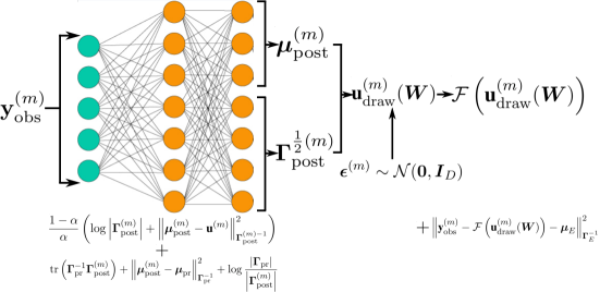
Figure 1: Schematic of the UQ-VAE framework with the exact PtO map.

During the training procedure, the repeated operation of the PtO map on our dataset $\left\{\left(\textbf{u}^{(m)},\textbf{y}_{\mathrm{obs}}^{(m)}\right)\right\}_{m=1}^{M}$ may incur a significant computational cost. To alleviate this, we also consider a modification to the optimization problem (21) where we simultaneously learn the PtO map along with the inverse problem solver. To this end, we replace the PtO map $\mathcal{F}$ with another neural network $\Psi_{\mathrm{d}}$ parameterized by weights $\boldsymbol{W}_{\mathrm{d}}$. With this, the term (21b) becomes

$$\left\lVert\textbf{y}_{\mathrm{obs}}^{(m)}-\Psi_{\mathrm{d}}\left(\textbf{u}_{\mathrm{draw}}^{(m)}(\boldsymbol{W}),\boldsymbol{W}_{\mathrm{d}}\right)-\boldsymbol{\mu}_{E}\right\rVert_{\boldsymbol{\Gamma}_{E}^{-1}}^{2}$$ (22)

and (21) becomes an optimization problem over both sets of weights $\left(\boldsymbol{W},\boldsymbol{W}_{\mathrm{d}}\right)$. Notice that the resulting optimization problem resembles those typically used to train an autoencoder. It is for this reason that we elect to use the subscript ‘d’ to indicate the decoder. Since the learned model $\Psi_{\mathrm{d}}$ of the PtO map $\mathcal{F}$ is a neural network, the evaluation of this map during the training phase is computationally inexpensive. However, this efficiency comes at the expense of utilizing knowledge of the governing physics of the inverse problems. Thus, the modified framework is almost purely data-driven and resembles more the original utility of VAEs for generative modelling. A schematic of the UQ-VAE framework with learned PtO map is displayed in Figure 2.

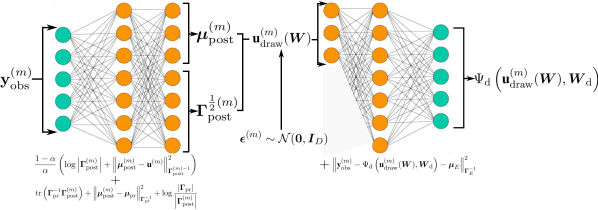
Figure 2: Schematic of the UQ-VAE framework with learned PtO map.

3.3 Analytical Result

We now present theoretical justification for the model-constrained UQ-VAE framework for the case where the PtO map $\mathcal{F}$ is linear. In this case, the target posterior $p(\textbf{u}|\textbf{y}_{\mathrm{obs}})$ is Gaussian provided that the prior model $\mathcal{N}(\boldsymbol{\mu}_{\mathrm{pr}},\boldsymbol{\Gamma}_{\mathrm{pr}})$ and noise model $\mathcal{N}(\boldsymbol{\mu}_{E},\boldsymbol{\Gamma}_{E})$ are also Gaussian. We show that linear, one-layer neural networks outputting the posterior mean and Cholesky factor of the posterior covariance are able to recover exactly the target posterior. The proof is given in Section A.2 of the Appendix.

Theorem 3.4.

Let $\textbf{y}_{\mathrm{obs}}\in\mathbb{R}^{O}$. Consider a Gaussian prior model $\mathcal{N}\left(\boldsymbol{\mu}_{\mathrm{pr}},\boldsymbol{\Gamma}_{\mathrm{pr}}\right)$ and Gaussian noise model $\mathcal{N}\left(\boldsymbol{\mu}_{E},\boldsymbol{\Gamma}_{E}\right)$. Suppose the target posterior $p(\textbf{u}|\textbf{y}_{\mathrm{obs}})=\mathcal{N}\left(\boldsymbol{\mu}_{\mathrm{true}},\boldsymbol{\Gamma}_{\mathrm{true}}\right)$ is such that

$$\boldsymbol{\Gamma}_{\mathrm{true}} =\left(\boldsymbol{F}^{\mathrm{T}}\boldsymbol{\Gamma}_{E}^{-1}\boldsymbol{F}+\boldsymbol{\Gamma}_{\mathrm{pr}}^{-1}\right)^{-1}$$ (23a)

$$\boldsymbol{\mu}_{\mathrm{true}} =\boldsymbol{\Gamma}_{\mathrm{true}}\left(\boldsymbol{F}^{\mathrm{T}}\boldsymbol{\Gamma}_{E}^{-1}\left(\textbf{y}_{\mathrm{obs}}-\boldsymbol{\mu}_{E}\right)+\boldsymbol{\Gamma}_{\mathrm{pr}}^{-1}\boldsymbol{\mu}_{\mathrm{pr}}\right)$$ (23b)

where $\boldsymbol{F}\in\mathbb{R}^{O\times D}$. Suppose the model posterior $q_{\boldsymbol{\phi}}(\textbf{u}|\textbf{y}_{\mathrm{obs}})=\mathcal{N}\left(\boldsymbol{\mu}_{\mathrm{post}},\boldsymbol{\Gamma}_{\mathrm{post}}\right)$ is such that

$$\boldsymbol{\mu}_{\mathrm{post}} =\boldsymbol{W}_{\boldsymbol{\mu}}\textbf{y}_{\mathrm{obs}}+\boldsymbol{b}_{\boldsymbol{\mu}}$$ (24a)

$$\boldsymbol{\Gamma}_{\mathrm{post}}^{\frac{1}{2}} =\boldsymbol{L}\odot\boldsymbol{L}_{\mathds{1}}+\mathrm{diag}\left(\boldsymbol{\sigma}\right)$$ (24b)

$$\log\left(\boldsymbol{\sigma}\right) =\boldsymbol{W}_{\boldsymbol{\sigma}}\textbf{y}_{\mathrm{obs}}+\boldsymbol{b}_{\boldsymbol{\sigma}}$$ (24c)

$$\mathrm{vec}\left(\boldsymbol{L}\right) =\boldsymbol{W}_{\boldsymbol{L}}\textbf{y}_{\mathrm{obs}}+\boldsymbol{b}_{\boldsymbol{L}}$$ (24d)

where $\boldsymbol{L}_{\mathds{1}}$ is a lower triangular matrix of ones with zeros on the diagonal. Let $\alpha=\frac{1}{2}$. Then the optimization problem

$$\min_{\boldsymbol{W}_{\boldsymbol{\mu}},\boldsymbol{b}_{\boldsymbol{\mu}},\boldsymbol{W}_{\boldsymbol{\sigma}},\boldsymbol{b}_{\boldsymbol{\sigma}},\boldsymbol{W}_{\boldsymbol{L}},\boldsymbol{b}_{\boldsymbol{L}}} \frac{1-\alpha}{\alpha}\left(\log\left|\boldsymbol{\Gamma}_{\mathrm{post}}\right|+\mathrm{tr}\left(\boldsymbol{\Gamma}_{\mathrm{post}}^{-1}\boldsymbol{\Gamma}_{\mathrm{true}}\right)+\left\|\boldsymbol{\mu}_{\mathrm{post}}-\boldsymbol{\mu}_{\mathrm{true}}\right\|_{\boldsymbol{\Gamma}_{\mathrm{post}}^{-1}}^{2}\right)$$ (25a)

$$+\mathrm{tr}\left(\boldsymbol{\Gamma}_{E}^{-1}\boldsymbol{F}\boldsymbol{\Gamma}_{\mathrm{post}}\boldsymbol{F}^{\mathrm{T}}\right)+\left\lVert\textbf{y}_{\mathrm{obs}}-\boldsymbol{F}\boldsymbol{\mu}_{\mathrm{post}}-\boldsymbol{\mu}_{E}\right\rVert_{\boldsymbol{\Gamma}_{E}^{-1}}^{2}$$ (25b)

$$+\mathrm{tr}\left(\boldsymbol{\Gamma}_{\mathrm{pr}}^{-1}\boldsymbol{\Gamma}_{\mathrm{post}}\right)+\left\|\boldsymbol{\mu}_{\mathrm{post}}-\boldsymbol{\mu}_{\mathrm{pr}}\right\|_{\boldsymbol{\Gamma}_{\mathrm{pr}}^{-1}}^{2}+\log\frac{\left|\boldsymbol{\Gamma}_{\mathrm{pr}}\right|}{\left|\boldsymbol{\Gamma}_{\mathrm{post}}\right|}$$ (25c)

achieves its minimum if and only if $\boldsymbol{W}_{\boldsymbol{\mu}},\boldsymbol{b}_{\boldsymbol{\mu}},\boldsymbol{W}_{\boldsymbol{\sigma}},\boldsymbol{b}_{\boldsymbol{\sigma}},\boldsymbol{W}_{\boldsymbol{L}},\boldsymbol{b}_{\boldsymbol{L}}$ are such that $\boldsymbol{\mu}_{\mathrm{post}}=\boldsymbol{\mu}_{\mathrm{true}}$ and $\boldsymbol{\Gamma}_{\mathrm{post}}=\boldsymbol{\Gamma}_{\mathrm{true}}$.

Although this result provides theoretical guarantees, the requirement of learning a full matrix in (24d) can be computational infeasible. For this reason, it is often the case that only the diagonal of the model posterior covariance is learned [Kingma and Welling(2013)].

4 Related Work

In generative modelling, it is beneficial to learn better representations of the latent space. To this end, the use of the JSD for VAEs is explored in [Deasy et al.(2020)Deasy, Simidjievski, and Liò, Sutter et al.(2020)Sutter, Daunhawer, and Vogt]. These works consider using the JSD in place of the KLD in the ELBO between the posterior and the prior. Our work differs from these approaches as the JSD is applied not directly to the ELBO. Rather, the JSD is applied at the inference level to yield a different bound that includes an expression of the latent data.

In scientific inverse problems, neural networks have been used to augment the solution process in [Adler and Öktem(2017), Jin et al.(2017)Jin, McCann, Froustey, and Unser, Li et al.(2018)Li, Schwab, Antholzer, and Haltmeier, Patel and Oberai(2019), Peng et al.(2020)Peng, Jalali, and Yuan, Seo et al.(2019)Seo, Kim, Jargal, Lee, and Harrach, Sheriffdeen et al.(2019)Sheriffdeen, Ragusa, Morel, Adams, and Bui-Thanh]. Some of these works use deep learning to assist a more traditional solution algorithm. In [Adler and Öktem(2017)], a convolutional neural network is used in a partially learned gradient descent scheme. In [Jin et al.(2017)Jin, McCann, Froustey, and Unser], the component of the iterative solution algorithm requiring convolutional operators is surrogated with convolutional neural networks. Other approaches use deep learning directly for regularization of an ill-posed inverse problem. In [Li et al.(2018)Li, Schwab, Antholzer, and Haltmeier], neural networks are used in place of a Tikhonov regularizer. The work in [Patel and Oberai(2019), Gonzalez et al.(2019)Gonzalez, Almansa, Delbracio, Musé, and Tan], explored prior modelling in Bayesian inverse problems using generative adversarial networks (GANs) and VAEs respectively. In [Seo et al.(2019)Seo, Kim, Jargal, Lee, and Harrach], VAEs are used to learn a low dimensional manifold representation of the PoI which introduces regularization for ill-posed inverse problems. Similarly, in [Peng et al.(2020)Peng, Jalali, and Yuan], an autoencoder is used to learn a latent representation of the unknown of interest which thereby allows the inversion task to be reframed into solving for the latent representation. In [Sheriffdeen et al.(2019)Sheriffdeen, Ragusa, Morel, Adams, and Bui-Thanh], bounded neural network discrepancy models were used to augment reduce order models in order to accelerate PDE-constrained inverse solutions. In summary, even with improvements through deep learning, the computational cost of these approaches is still mostly inherited from the cost of the base solution algorithms that were augmented. In our approach, the solution process is itself propagation through a trained neural network; a process largely unrivalled in terms of computational efficiency. Additionally, most of the work mentioned above do not quantify uncertainty.

Broadly speaking, there are three types of approaches for performing UQ with deep learning. In an analogous manner to above, the first type utilizes deep learning to augment traditional methods for UQ. In [Jiang et al.(2019)Jiang, Zhang, Turnadge, and Xu], an autoencoder is trained to reduce the dimensionality of the PoI space. MCMC sampling is then conducted on the low-dimensional representation and estimation in the full PoI space is recovered by propagation through the trained decoder. Similarly, in [Hou et al.(2019)Hou, Lam, Zhang, and Zhang], a class of network training methods was proposed that can be combined with sample-based Bayesian inference algorithms. For the second type of approach, deep learning models that inherently possess some stochastic property are, themselves, used to represent uncertainty. In [Caldeira and Nord(2020)], an investigation into Bayesian Neural Networks, Concrete Dropout and Deep Ensembles was provided in the setting of scientific problems. However, the discussion in the paper does not directly pertain to inverse problems.

Our proposed method for UQ falls under the third type of approach. Here, deep learning is used to directly learn and model the uncertainty. In [Gabbard et al.(2019)Gabbard, Messenger, Heng, Tonolini, and Murray-Smith, Tonolini et al.(2020)Tonolini, Radford, Turpin, Faccio, and Murray-Smith, Chua and Vallisneri(2020), Adler and Öktem(2018)], purely deep learning posterior modelling approaches were proposed. In [Gabbard et al.(2019)Gabbard, Messenger, Heng, Tonolini, and Murray-Smith] and [Tonolini et al.(2020)Tonolini, Radford, Turpin, Faccio, and Murray-Smith], conditional VAEs (CVAE) [Sohn et al.(2015)Sohn, Lee, and Yan] were trained to perform variational inference for gravitational-wave astronomy problems and computational imaging problems respectively. Unlike our UQ-VAE approach, CVAEs do not marry the latent space with the PoI space; they require a separate latent variable for its derivation. The work in [Chua and Vallisneri(2020)] trains a neural network to rapidly produce one or two dimensional projections of Bayesian posteriors for gravitational-wave astronomy. For more general and higher-dimensional settings, the work in [Adler and Öktem(2018)] introduces Deep Posterior Sampling which trains a Wasserstein GAN to sample from the posterior. However, the training of GANs is notoriously unstable; a limitation also met and acknowledged by the authors of [Adler and Öktem(2018)] in their paper. Compared to GANs, VAEs possess a mathematical rigour that is more directly related to the data distribution it attempts to generate from. Therefore, with the VAE at the core of our proposed framework, we postulate that there is more potential for mathematically rigourous extension.

5 Results

For our numerical experiments, we consider the two dimensional steady state heat conduction problem. The details of this problem setup can be found in Section B of the Appendix. Although the non-linear forward mapping is quite simple, elliptic inverse problems are severely ill-posed and serve as excellent benchmark inference problems [Kabanikhin(2008), Kirsch(2011), Beskos et al.(2017)Beskos, Girolami, Lan, Farrell, and Stuart, Cui et al.(2016)Cui, Law, and Marzouk, Chen et al.(2019)Chen, Wu, Chen, O’Leary-Roseberry, and Ghattas]. Details of the neural network architectures and optimization procedure can be found in Section C of the Appendix. The codes implementing the UQ-VAE framework used to produce these results can be obtained from [Goh(2020)]. For comparison, we use the hIPPYlib library [Villa et al.(2019)Villa, Petra, and Ghattas] to compute the Laplace approximation using gradients and Hessians derived via the adjoint method, inexact Newton-CG, Armijo line search and randomized eigensolvers.

For our numerical experiments, we consider the following cases:

1. four noise levels $\eta=0,0.01,0.05,0.1$

2. four sizes of training datasets $M=50,500,1000,5000$

3. four choices of the JSD family $\alpha=0.00001,0.001,0.1,0.5$

4. exact PtO map and learned PtO map.

For our numerical simulations, in some cases, selecting $\alpha\geq 0.5$ may yield an unstable training procedure with exploding gradients and so we only display results with $\alpha$ as high as $\alpha=0.5$. The computational cost of training is detailed in Section C.3 of the Appendix. The table of relative errors and figures are found in Section D of the Appendix with each figure set and subsection representing a noise level and dataset size. Note that we have elected to only display the cross-sectional predictions and not the predictions over the full domain since it is harder to visualize the uncertainty in the latter.

Before continuing to a detailed discussion, we address the comment in Section 3.2 regarding the adoption of a crude Monte-Carlo approximation using our PoI data. The overall feasibility of our obtained uncertainty estimates indicate that it is sufficient to use only one PoI datapoint. We postulate that any inaccuracies resulting from such a crude approximation is alleviated by the variety of information embedded in the training dataset. Indeed, since the weights are used to capture the statistics of a whole training dataset, the amortized nature of our inference method perhaps reduces the requirement for accurate Monte-Carlo approximations. Moreover, in the original VAE paper [Kingma and Welling(2013)], the authors observed that, providing the number of training data $M$ was large enough, using only one draw from the model posterior to approximate the expected value of the likelihood term was sufficient to obtain good results. This finding regarding the approximation of the likelihood term mirrors ours regarding the posterior data misfit term.

5.1 Comparison with the Laplace Approximation

We summarize our results beginning with a comparison between UQ using UQ-VAE and with the Laplace approximation. It is important to point out that UQ-VAE provides a global Gaussian approximation while the Laplace approximation is usually a local Gaussian approximation at the MAP point. From the results, we can see that the posterior mean estimated by the UQ-VAE is closer to the true value than the MAP estimate. However, the Laplace approximation provides larger uncertainty estimates which ensures they are still feasible despite the underestimation of values by the MAP. In contrast, especially for larger values of $\alpha$, the UQ-VAE uncertainty estimates are smaller and, in some cases, the true parameter values at the location of the anomaly lie slightly outside the uncertainty estimates.

Recall that the statistics of the noise are accurately modelled. Therefore, the larger the value of $\eta$, the more diminished the influence of the likelihood model (21b) on the training procedure; through penalization by the weighting matrix $\boldsymbol{\Gamma}_{E}^{-1}$. For the Laplace approximation (12), this translates to an increase in the approximate posterior variance. The approximate posterior variance obtained from the UQ-VAE also exhibits this response to the increased noise regularization.

Further, the Laplace approximation uncertainty estimates are clearly responsive to the sensor locations; providing smaller uncertainty where the sensors are located. Whilst the UQ-VAE uncertainty estimates do exhibit a similar behaviour, it is less pronounced due to the aforementioned global and local nature of the UQ-VAE and Laplace approximation, respectively. Furthermore, we postulate that this is because the UQ-VAE uncertainty estimates represent two sources of information; the observational data fed into the encoder as well as the PoI and observational pairs in the training dataset. Whilst the former provides information only at the locations at the sensors, the latter provides information at all areas of the domain. Indeed, the process of training under the UQ-VAE framework works to embed information about the training dataset into the neural network. UQ is then performed with this embedded information as well as the input observational data. Despite these differences, we believe that it is still instructive to compare the two approximations.

Finally, the computational efficiency of inference by propagation through a trained neural network $\Psi$ is, on average, more than 2750 times faster than that of the Laplace approximation.

See Section C.3 of the Appendix for more details on the computational cost of inference. An example of our computational results is displayed in Figure 3 which compares the uncertainty estimates obtained using the Laplace approximation with those obtained with our UQ-VAE framework.

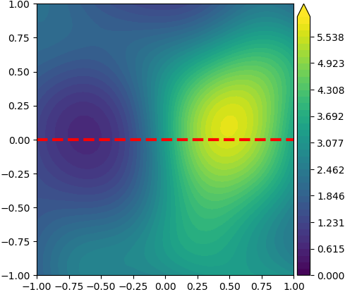
Figure 3: Top row left to right: mesh with sensors denoted with a red cross, true PoI, cross-sectional uncertainty estimate and pointwise posterior variance from Laplace approximation. Second row: UQ-VAE uncertainty estimates with $\alpha=0.001$. First and third columns: cross-sectional uncertainty estimates. Second and fourth columns: approximate pointwise posterior variance. First and second columns: exact PtO map. Third and fourth columns: learned PtO map.

5.2 Comparison Within the UQ-VAE Framework

Now, we discuss the results within the UQ-VAE framework by comparing between noise levels, dataset size, modelling and learning of the PtO map and choices of $\alpha$:

1. Comparing between noise levels, feasible estimates were obtained for all noise levels. However, for $\eta=0.05$, feasible estimates were only obtained for $M=50,500,1000$. With the exception of $\eta=0.05$ and $M=5000$, the uncertainty estimates are larger for larger values of $\eta$. For the noise level of $\eta=0.1$, no feasible estimates were obtained for any choice of dataset size $M$.

2. Comparing between training dataset sizes, the uncertainty estimates are larger for smaller dataset sizes. When $\eta=0.05$, larger dataset sizes appear to be detrimental to the accuracy of the estimation.

3. Comparing between the case where the PtO is exact and when the PtO is learned, for the cases of $\eta=0$, $M=500$, $\alpha=0.5$ and $\eta=0.01$, $M=500$, $\alpha=0.1$, using the exact PtO clearly outperforms using the learned PtO.

4. Comparing between choices of $\alpha$, for smaller values of $\alpha$ the estimated posterior mean underestimates the true PoI values and so a larger uncertainty estimate is required to ensure feasible estimates. The reverse occurs for larger values of $\alpha$.

We now offer some key interpretations our above observations. For the first observation, the reasoning for larger uncertainty estimates observed with larger values of $\eta$ was discussed in Section 5.1.

For the second observation, we see that the posterior uncertainty is responsive to the size of the dataset. With less data, our uncertainty estimates are larger. This behaviour is ideal as more information intuitively implies less uncertainty. For the case of $\eta=0.05$, we conjecture that the use of large datasets of heavily corrupted data yields an unfavourable influence on our optimization procedure. We believe that the limitation of our framework lies in its potential dependence on an accurate training dataset. One of the key merits of our proposed method is that we have introduced, in a mathematically justified manner, a data-driven component to the inversion process. This expands the toolkit at one’s disposal when solving inverse problems. Indeed, in addition to constructing models for the prior and the PtO map, information on the properties of the PoI as well as the governing physics can be encoded into the training dataset. However, it would be incomplete to view this added option purely as an advantage. Although the utilization of datasets alleviates the burden on accurate prior and physics modelling, poorly constructed or highly corrupted datasets could completely sabotage the inversion process regardless of any accuracy achieved by the prior and physics models.

For the third observation, it can be reasoned that the similarity of results for the two cases is due to the success of the decoder in learning the PtO. The elliptic forward problem is quite simple and so it is not unexpected that the decoder learns it with ease. Thus, simultaneously learning an accurate PtO may be a reasonable task that aids and does not detract from the main task of learning the Bayesian inverse problems solver. This supports the strategy of using a learned PtO to reduce the offline cost of training the neural network. However, the two cases where use of the exact PtO outperforms using the learned PtO with the small training dataset size of $M=500$ suggests that including the physics of the problem allows for feasible uncertainty estimates when large amounts of training data may not be readily available.

For the fourth observation, in alignment with our discussion in Section 3.2, a lower value of $\alpha$ creates a larger penalty on the posterior terms (21a). Since our results suggest that a lower value of $\alpha$ yields a larger posterior variance, then it is implied that the minimization of $\log\left|\boldsymbol{\Gamma}_{\mathrm{post}}^{(m)}\right|$ is not a priority during the training procedure; so long as the posterior data $\textbf{u}^{(m)}$ has enough influence. One can also reason that since lower values of $\alpha$ correspond to the zero-forcing KLD, one would expect a larger model variance; for example in the case of approximating a multimodal distribution with a unimodal model [Bishop(2006)]. The reverse occurs with higher values of $\alpha$ which, due to tendency towards the zero-avoiding KLD, would result in a smaller model variance.

Finally, we address the instability of the training procedure as $\alpha\to 1$ which diminishes the influence of the PoI data on our optimization problem and moves towards recovering the zero-avoiding KLD. Recall the more traditional method of optimizing the exponentiated functional in (11) where the target optimization parameter is the physically meaningful u. In contrast, our method optimizes for the more arbitrary and often more plentiful weights $\boldsymbol{W}$. Intuitively, we are therefore faced with a more ill-posed problem. Moreover, from a perspective centered around the traditional posterior (11), one can instead view the posterior data terms (21a) as regularizers of the traditional loss functional involving only the likelihood and prior term. This provides the much needed regularization for our more ill-posed inverse problem; which therefore necessitates that $\alpha\ll 1$ for this regularization to take effect. We leave concrete theoretical analysis for future work.

6 Conclusion

In this paper, we propose a framework for training of neural networks capable of rapid UQ. Although the VAE, on which this framework is based, was originally motivated by methods in generative modelling, we have shown that it is also well suited for scientific inverse problems. Indeed, it utilizes three sources of information usually available for such problems:

1. the physical laws governing the problem through the PtO map

2. the physical properties of the PoI through the prior model

3. simulation or experimentation procedures through the paired PoI-observation datasets.

Furthermore, this framework is derived from a solid mathematical foundation and possesses a complex, dynamic interplay of factors from variational inference as well as regularization. Despite this complexity, this framework requires only a few design decisions. Indeed, aside from the usual adjustment of hyperparameters associated with neural network architecture, essentially only the tuning of the hyperparameter $\alpha$ is required. The selection of the PtO map and prior model can be guided by the underlying physical properties of the problem. Our results also show that feasible estimates are achievable and, moreover, that these estimates exhibit behaviour similar to that of existing inversion methods. Additionally, our uncertainty estimates show a favourable response to the size of our training dataset; the uncertainty is inversely proportional to the amount of training data used which reflects the availability or lack of information. The preliminary investigation offered in this paper employs only standard optimization techniques and simple deep learning architectures with a very minimal amount of tuning performed. This decision was made in order to showcase the robustness as well as the limitations of our framework in its most basic form. Moreover, we utilize somewhat crude statistical approximations. We believe that the results presented in this paper can be improved with the employment of more sophisticated optimization procedures, neural network architecture and statistical machinery.

This research was partially funded by the National Science Foundation awards NSF-1808576 and NSF-CAREER-1845799; by the Defense Thread Reduction Agency award DTRA-M1802962; by the Department of Energy award DE-SC0018147; by KAUST; by 2018 ConTex award; and by 2018 UT-Portugal CoLab award. The authors acknowledge the Texas Advanced Computing Center (TACC) at The University of Texas at Austin for providing HPC resources that have contributed to the research results reported within this paper. URL: http://www.tacc.utexas.edu. The authors would like to thank Jari Kaipio, Ruanui Nicholson and Rory Wittmer for the insightful discussions.

Appendix A Proofs

A.1 Proof of Theorem 3.1

Proof A.1.

The clearest path forward is to manipulate

$$\mathrm{JS}_{\alpha}(q_{\boldsymbol{\phi}}(\textbf{u}|\textbf{y})||p(\textbf{u}|\textbf{y}))= \alpha\mathrm{KL}(q_{\boldsymbol{\phi}}(\textbf{u}|\textbf{y})||(1-\alpha)q_{\boldsymbol{\phi}}(\textbf{u}|\textbf{y})+\alpha p(\textbf{u}|\textbf{y}))$$ (26a)

$$+(1-\alpha)\mathrm{KL}(p(\textbf{u}|\textbf{y})||(1-\alpha)q_{\boldsymbol{\phi}}(\textbf{u}|\textbf{y})+\alpha p(\textbf{u}|\textbf{y}))$$ (26b)

term-by-term. Beginning with the first term,

$$\alpha\mathrm{KL}(q_{\boldsymbol{\phi}}(\textbf{u}|\textbf{y})||(1-\alpha)q_{\boldsymbol{\phi}}(\textbf{u}|\textbf{y})+\alpha p(\textbf{u}|\textbf{y}))$$ (27a)

$$=\alpha\mathbb{E}_{\textbf{u}\sim q_{\boldsymbol{\phi}}}\left[\log\left(\frac{q_{\boldsymbol{\phi}}(\textbf{u}|\textbf{y})}{(1-\alpha)q_{\boldsymbol{\phi}}(\textbf{u}|\textbf{y})+\alpha p(\textbf{u}|\textbf{y})}\right)\right]$$ (27b)

$$=-\alpha\mathbb{E}_{\textbf{u}\sim q_{\boldsymbol{\phi}}}\left[\log\left(\frac{(1-\alpha)q_{\boldsymbol{\phi}}(\textbf{u}|\textbf{y})+\alpha p(\textbf{u}|\textbf{y})}{q_{\boldsymbol{\phi}}(\textbf{u}|\textbf{y})}\right)\right]$$ (27c)

$$=-\alpha\mathbb{E}_{\textbf{u}\sim q_{\boldsymbol{\phi}}}\left[\log\left(\frac{p(\textbf{u}|\textbf{y})}{q_{\boldsymbol{\phi}}(\textbf{u}|\textbf{y})}\left(\alpha+\frac{(1-\alpha)q_{\boldsymbol{\phi}}(\textbf{u}|\textbf{y})}{p(\textbf{u}|\textbf{y})}\right)\right)\right]$$ (27d)

$$=-\alpha\mathbb{E}_{\textbf{u}\sim q_{\boldsymbol{\phi}}}\left[\log\left(\frac{p(\textbf{u}|\textbf{y})}{q_{\boldsymbol{\phi}}(\textbf{u}|\textbf{y})}\right)\right]-\alpha\mathbb{E}_{\textbf{u}\sim q_{\boldsymbol{\phi}}}\left[\log\left(\alpha+\frac{(1-\alpha)q_{\boldsymbol{\phi}}(\textbf{u}|\textbf{y})}{p(\textbf{u}|\textbf{y})}\right)\right]$$ (27e)

$$=-\alpha\mathbb{E}_{\textbf{u}\sim q_{\boldsymbol{\phi}}}\left[\log\left(\frac{p(\textbf{y},\textbf{u})}{p(\textbf{y})q_{\boldsymbol{\phi}}(\textbf{u}|\textbf{y})}\right)\right]-\alpha\mathbb{E}_{\textbf{u}\sim q_{\boldsymbol{\phi}}}\left[\log\left(\alpha+\frac{(1-\alpha)q_{\boldsymbol{\phi}}(\textbf{u}|\textbf{y})}{p(\textbf{u}|\textbf{y})}\right)\right]$$ (27f)

$$=\alpha\log\left(p(\textbf{y})\right)-\alpha\mathbb{E}_{\textbf{u}\sim q_{\boldsymbol{\phi}}}\left[\log\left(\frac{p(\textbf{y},\textbf{u})}{q_{\boldsymbol{\phi}}(\textbf{u}|\textbf{y})}\right)\right]-\alpha\mathbb{E}_{\textbf{u}\sim q_{\boldsymbol{\phi}}}\left[\log\left(\alpha+\frac{(1-\alpha)q_{\boldsymbol{\phi}}(\textbf{u}|\textbf{y})}{p(\textbf{u}|\textbf{y})}\right)\right].$$ (27g)

Similarly, the second term can be decomposed as

$$(1-\alpha)\mathrm{KL}(p(\textbf{u}|\textbf{y})||(1-\alpha)q_{\boldsymbol{\phi}}(\textbf{u}|\textbf{y})+\alpha p(\textbf{u}|\textbf{y}))$$ (28a)

$$=(1-\alpha)\mathbb{E}_{\textbf{u}\sim p(\textbf{u}|\textbf{y})}\left[\log\left(\frac{p(\textbf{u}|\textbf{y})}{(1-\alpha)q_{\boldsymbol{\phi}}(\textbf{u}|\textbf{y})+\alpha p(\textbf{u}|\textbf{y})}\right)\right]$$ (28b)

$$=-(1-\alpha)\mathbb{E}_{\textbf{u}\sim p(\textbf{u}|\textbf{y})}\left[\log\left(\frac{(1-\alpha)q_{\boldsymbol{\phi}}(\textbf{u}|\textbf{y})+\alpha p(\textbf{u}|\textbf{y})}{p(\textbf{u}|\textbf{y})}\right)\right]$$ (28c)

$$=-(1-\alpha)\mathbb{E}_{\textbf{u}\sim p(\textbf{u}|\textbf{y})}\left[\log\left(\alpha+\frac{(1-\alpha)q_{\boldsymbol{\phi}}(\textbf{u}|\textbf{y})}{p(\textbf{u}|\textbf{y})}\right)\right].$$ (28d)

Combining equations (27) and (28), we arrive at

$$\mathrm{JS}_{\alpha}(q_{\boldsymbol{\phi}}(\textbf{u}|\textbf{y})||p(\textbf{u}|\textbf{y}))= \alpha\log\left(p(\textbf{y})\right)$$ (29a)

$$-\alpha\mathbb{E}_{\textbf{u}\sim q_{\boldsymbol{\phi}}}\left[\log\left(\frac{p(\textbf{y},\textbf{u})}{q_{\boldsymbol{\phi}}(\textbf{u}|\textbf{y})}\right)\right]$$ (29b)

$$-\alpha\mathbb{E}_{\textbf{u}\sim q_{\boldsymbol{\phi}}}\left[\log\left(\alpha+\frac{(1-\alpha)q_{\boldsymbol{\phi}}(\textbf{u}|\textbf{y})}{p(\textbf{u}|\textbf{y})}\right)\right]$$ (29c)

$$-(1-\alpha)\mathbb{E}_{\textbf{u}\sim p(\textbf{u}|\textbf{y})}\left[\log\left(\alpha+\frac{(1-\alpha)q_{\boldsymbol{\phi}}(\textbf{u}|\textbf{y})}{p(\textbf{u}|\textbf{y})}\right)\right].$$ (29d)

Finally, the expressions in Theorem 3.1 follow through division by $\alpha$ and rearrangement.

A.2 Proof of Theorem 3.4

Proof A.2.

Set $\alpha=\frac{1}{2}$. Forcing the variations with respect to weights $\boldsymbol{W}_{\boldsymbol{\mu}}$ and biases $\boldsymbol{b}_{\boldsymbol{\mu}}$ to vanish gives

$$\boldsymbol{\Gamma}_{\mathrm{post}}^{-1}\left(\boldsymbol{\mu}_{\mathrm{post}}-\boldsymbol{\mu}_{\mathrm{true}}\right)$$ (30a)

$$-\boldsymbol{F}^{\mathrm{T}}\boldsymbol{\Gamma}_{E}^{-1}\left(\textbf{y}_{\mathrm{obs}}-\boldsymbol{F}\boldsymbol{\mu}_{\mathrm{post}}-\boldsymbol{\mu}_{E}\right)+\boldsymbol{\Gamma}_{\mathrm{pr}}^{-1}\left(\boldsymbol{\mu}_{\mathrm{post}}-\boldsymbol{\mu}_{\mathrm{pr}}\right)$$ (30b)

$$=\textbf{0}$$ (30c)

which is true if and only if $\boldsymbol{\mu}_{\mathrm{post}}=\boldsymbol{\mu}_{\mathrm{true}}$. Forcing the variations with respect to $\boldsymbol{W}_{\boldsymbol{L}}$ and biases $\boldsymbol{b}_{\boldsymbol{L}}$ to vanish gives

$$-\left(\boldsymbol{\Gamma}_{\mathrm{post}}^{-\frac{1}{2}}\boldsymbol{\Gamma}_{\mathrm{true}}\otimes\boldsymbol{\Gamma}_{\mathrm{post}}^{-\frac{1}{2}\mathrm{T}}+\boldsymbol{\Gamma}_{\mathrm{post}}^{-\frac{1}{2}}\left(\boldsymbol{\mu}_{\mathrm{post}}-\boldsymbol{\mu}_{\mathrm{true}}\right)\left(\boldsymbol{\mu}_{\mathrm{post}}-\boldsymbol{\mu}_{\mathrm{true}}\right)^{\mathrm{T}}\otimes\boldsymbol{\Gamma}_{\mathrm{post}}^{-\frac{1}{2}\mathrm{T}}\right)\mathrm{vec}\left(\boldsymbol{\Gamma}_{\mathrm{post}}^{-\frac{1}{2}}\right)$$ (31a)

$$+\left(\boldsymbol{I}_{D}\otimes\boldsymbol{F}^{\mathrm{T}}\boldsymbol{\Gamma}_{E}^{-1}\boldsymbol{F}\right)\mathrm{vec}\left(\boldsymbol{\Gamma}_{\mathrm{post}}^{\frac{1}{2}}\right)+\left(\boldsymbol{I}_{D}\otimes\boldsymbol{\Gamma}_{\mathrm{pr}}^{-1}\right)\mathrm{vec}\left(\boldsymbol{\Gamma}_{\mathrm{post}}^{\frac{1}{2}}\right)$$ (31b)

$$=\textbf{0}$$ (31c)

where $\otimes$ denotes the Kronecker product. Using the two identities [Dhrymes(1978)]

$$\mathrm{vec}\left(\boldsymbol{A}\boldsymbol{B}\boldsymbol{C}\boldsymbol{D}\right) =\left(\boldsymbol{D}^{\mathrm{T}}\boldsymbol{C}^{\mathrm{T}}\otimes\boldsymbol{A}\right)\mathrm{vec}\left(\boldsymbol{B}\right)$$ (32a)

$$\mathrm{vec}\left(\boldsymbol{A}\boldsymbol{B}\right) =\left(\boldsymbol{I}\otimes\boldsymbol{A}\right)\mathrm{vec}\left(\boldsymbol{B}\right)$$ (32b)

along with some basic manipulation gives

$$-\boldsymbol{\Gamma}_{\mathrm{post}}^{-1}\left(\boldsymbol{\Gamma}_{\mathrm{true}}+\left(\boldsymbol{\mu}_{\mathrm{post}}-\boldsymbol{\mu}_{\mathrm{true}}\right)\left(\boldsymbol{\mu}_{\mathrm{post}}-\boldsymbol{\mu}_{\mathrm{true}}\right)^{\mathrm{T}}\right)+\left(\boldsymbol{F}^{\mathrm{T}}\boldsymbol{\Gamma}_{E}^{-1}\boldsymbol{F}+\boldsymbol{\Gamma}_{\mathrm{pr}}^{-1}\right)\boldsymbol{\Gamma}_{\mathrm{post}}=\textbf{0}.$$ (33)

Forcing the variations with respect to $\boldsymbol{W}_{\boldsymbol{\sigma}}$ and biases $\boldsymbol{b}_{\boldsymbol{\sigma}}$ to vanish gives

$$-\boldsymbol{\Gamma}_{\mathrm{post}}^{-1}\odot\left(\boldsymbol{\Gamma}_{\mathrm{true}}+\left(\boldsymbol{\mu}_{\mathrm{post}}-\boldsymbol{\mu}_{\mathrm{true}}\right)\left(\boldsymbol{\mu}_{\mathrm{post}}-\boldsymbol{\mu}_{\mathrm{true}}\right)^{\mathrm{T}}\right)\boldsymbol{\Gamma}_{\mathrm{post}}^{-\frac{1}{2}\mathrm{T}}$$ (34a)

$$+\left(\boldsymbol{F}^{\mathrm{T}}\boldsymbol{\Gamma}_{E}^{-1}\boldsymbol{F}\odot\boldsymbol{\Gamma}_{\mathrm{post}}^{\frac{1}{2}}\right)+\left(\boldsymbol{\Gamma}_{\mathrm{pr}}^{-1}\odot\boldsymbol{\Gamma}_{\mathrm{post}}^{\frac{1}{2}}\right)$$ (34b)

$$=\textbf{0}$$ (34c)

where $\odot$ denotes the entrywise product. Here, (33) and (34) with $\boldsymbol{\mu}_{\mathrm{post}}=\boldsymbol{\mu}_{\mathrm{true}}$ are true if and only if $\boldsymbol{\Gamma}_{\mathrm{post}}=\boldsymbol{\Gamma}_{\mathrm{true}}$ as required.

Appendix B Two Dimensional Steady State Heat Conduction Problem

We considered the heat equation with heat conductivity as the PoI and temperature as the state. The governing PDE and associated boundary conditions are displayed below

$$-\nabla\cdot u\nabla y =0 \quad\text{ in }\Omega$$ (35a)

$$-u(\nabla y\cdot\hat{\textbf{n}}) =\mathrm{Bi}\,y \quad\text{ on }\Omega^{\mathrm{ext}}\setminus\Omega^{\mathrm{root}}$$ (35b)

$$-u(\nabla y\cdot\hat{\textbf{n}}) =-1 \quad\text{ on }\Omega^{\mathrm{root}}$$ (35c)

where $u$ denotes the thermal heat conductivity, $\mathrm{Bi}$ is the Biot number set to $\mathrm{Bi}=0.5$, $\Omega$ is the physical domain, $\Omega^{\mathrm{root}}$ is the bottom edge of the domain and $\Omega^{\mathrm{ext}}$ is the remaining edges of the domain.

The prior model has mean $\boldsymbol{\mu}_{\mathrm{pr}}=2$ and covariance $\boldsymbol{\Gamma}_{\mathrm{pr}}$ that is a discretization of the infinite dimensional covariance operator $\mathcal{C}_{\mathrm{pr}}=\mathcal{A}^{-2}$ where $\mathcal{A}$ is a differential operator such that

$$\mathcal{A}u=\begin{cases}-\gamma\Delta u+\delta u&\text{ in }\Omega\\ \nabla u\cdot\hat{\textbf{n}}+\beta u&\text{ on }\partial\Omega.\end{cases}$$ (36)

Here, $\delta,\gamma>0$ controls the correlation length and variance of the prior operator. We set $\gamma=0.1$, $\delta=0.5$ and $\beta$ is chosen as in [Daon and Stadler(2016), Roininen et al.(2014)Roininen, Huttunen, and Lasanen] to reduce boundary artifacts. Priors of this type ensure that $\mathcal{C}_{\mathrm{pr}}$ is a trace-class operator which guarantees bounded pointwise variance and a well-posed infinite-dimensional Bayesian inverse problem [Stuart(2010), Bui-Thanh et al.(2013)Bui-Thanh, Ghattas, Martin, and Stadler].

The testing dataset of PoI values is drawn from a Gaussian autocorrelation smoothness prior [Kaipio and Somersalo(2006)] with mean $\boldsymbol{\mu}=2$ and covariance

$$\boldsymbol{\Gamma}_{ij}=\sigma^{2}\exp\left(-\frac{\left\lVert\textbf{x}_{i}-\textbf{x}_{j}\right\rVert_{2}^{2}}{2\rho^{2}}\right)$$ (37)

with $\sigma^{2}=2$, $\rho=0.5$. The training set for the UQ-VAE network is a set of separate draws from the same distribution. From this, the corresponding state observations are computed using the solvers from the FEniCS library [Logg et al.(2012)Logg, Mardal, and Wells] on the PoI dataset. The same solver is used as our numerical model of the PtO map during the training procedure.

We consider a computational domain consisting of $D=2601$ degrees of freedom. The observation data corresponds to sensor measurements from $10$ randomly selected locations and is afflicted with Gaussian distributed additive noise on all sensors with zero mean and standard deviation $\sigma=\eta\max\left|\textbf{y}_{\mathrm{obs}}\right|$. For our noise model, we set $\left(\boldsymbol{\mu}_{E},\boldsymbol{\Gamma}_{E}\right)=\left(\textbf{0},\sigma^{2}\boldsymbol{I}_{O}\right)$ which corresponds to the scenario where the statistics of the noise are accurately modelled. Finally, we assume a diagonal matrix for our posterior model covariance.

Appendix C Neural Network Architecture and Training Properties

C.1 Architecture

The architecture of our neural network $\Psi$ consists of $5$ hidden layers of $500$ nodes with the ReLU activation function. No activation function was used at the output layer. The input layer has $O$ number of nodes to match the dimension of the observational data which comprises of $O$ number of measurement points. The output layer has $2D$ nodes, with $D$ the dimension of the PoI, to represent the estimated posterior mean $\boldsymbol{\mu}_{\mathrm{post}}$ and diagonal of the posterior covariance $\boldsymbol{\Gamma}_{\mathrm{post}}$.

When the parameter-to-observable map is learnt, the corresponding decoder network $\Psi_{\mathrm{d}}$ has $2$ hidden layers also with $500$ nodes and the ReLU activation function. Again, no activation function was used at the output layer. The input layer has $D$ number of nodes to represent a draw from the learned posterior and the output layer has $O$ number of nodes to match the dimension of the observational data.

C.2 Training

For optimization, we use a batch size of $100$. Therefore, the loss in (21) is averaged over the number of PoI and observation pairs and the gradient is calculated for each batch. Optimization is conducted using the Adam optimizer which performs mini-batch momentum-based stochastic gradient descent [Kingma and Ba(2014)]. This training procedure was repeated for 400 epochs.

The metric used to measure accuracy is the averaged relative error $\frac{1}{L}\sum_{l=1}^{L}\frac{\left\lVert\textbf{u}^{(l)}-\boldsymbol{\mu}_{\mathrm{post}}\left(\textbf{y}_{\mathrm{obs}}^{(l)}\right)\right\rVert_{2}^{2}}{\left\lVert\textbf{u}^{(l)}\right\rVert_{2}^{2}}$ where $\left\{\left(\textbf{u}^{(l)},\textbf{y}_{\mathrm{obs}}^{(l)}\right)\right\}_{l=1}^{L}$ is a dataset unseen by the training procedure and $\boldsymbol{\mu}_{\mathrm{post}}\left(\textbf{y}_{\mathrm{obs}}^{(l)}\right)$ is the estimated posterior mean from the neural network $\Psi$ taking a datapoint $\textbf{y}_{\mathrm{obs}}^{(l)}$ as an input. An estimate is said to be feasible if and only if true value lies within the estimated uncertainty bounds. The uncertainty bounds displayed represent three standard deviations. Similarly, when the PtO map is learned by $\Psi_{\mathrm{d}}$, we use the relative error $\frac{1}{L}\sum_{l=1}^{L}\frac{\left\lVert\textbf{y}_{\mathrm{obs}}^{(l)}-\Psi_{\mathrm{d}}\left(\textbf{u}\left(\textbf{y}_{\mathrm{obs}}^{(l)}\right)\right)\right\rVert_{2}^{2}}{\left\lVert\textbf{y}_{\mathrm{obs}}^{(l)}\right\rVert_{2}^{2}}$ where $\textbf{u}\left(\textbf{y}_{\mathrm{obs}}^{(l)}\right)$ is a draw model posterior output by the trained encoder with a datapoint $\textbf{y}_{\mathrm{obs}}^{(l)}$ as an input.

C.3 Computational Cost

When training a neural network with the (21b) term in the loss functional (21) using the PtO map $\mathcal{F}$, the solving of a linear system is required. Because of this, training on CPUs is more efficient. In contrast, when the (21b) term uses the learned PtO map $\Psi_{\mathrm{d}}$ instead, no linear system solves are required and so the training procedure is most efficient on GPUs. We monitor the cost of training each batch as wall-clock time for the whole optimization procedure. The offline cost for training the networks using $\mathcal{F}$ is, on average, 4.5 seconds per batch on a dual-socket node with two Intel Xeon E5-2690 CPUs for a total of 24 cores. The offline cost for training the networks using $\Psi_{\mathrm{d}}$ is, on average, 0.35 seconds per batch on a NVIDIA 1080-TI GPU.

We compare the computational efficiency of inference between the Laplace approximation and propagation through the neural network $\Psi$ trained under the UQ-VAE framework on a Intel Core i7-8550U CPU using an average wall-clock time over 20 evaluations. The time taken to form the MAP estimate with hIPPYlib is, on average, 40 seconds with a maximum number of descent iterations of 25. The time taken to form the low-rank Gaussian approximation of the posterior covariance with 50 requested eigenvectors is, on average, 70 seconds. Therefore, in total, it takes on average 110 seconds to form the Laplace approximation. In contrast, forming the model posterior by propagation through a trained neural network takes, on average, 0.04 seconds; more than 2750 times faster.

Appendix D Results: Two Dimensional Steady State Heat Conduction Problem

D.1 $\eta=0$, $M=50$

	Relative Error: u		Relative Error: $\textbf{y}_{\mathrm{obs}}$
$\alpha$	Exact PtO	Learned PtO	Learned PtO
0.00001	28.88%	30.86%	24.61%
0.001	30.46%	30.76%	22.80%
0.1	30.70%	28.95%	49.38%
0.5	29.75%	32.73%	45.34%

Table 1: Table displaying the relative errors for UQ-VAE. Relative error of MAP estimate: 15.15%.

Figure 4: Top row left to right: mesh with sensors denoted with a red cross, true PoI, cross-sectional uncertainty estimate and pointwise posterior variance from Laplace approximation. Second to fourth rows: $\alpha=0.00001,0.001,0.1,0.5$. First and third columns: cross-sectional uncertainty estimates. Second and fourth columns: approximate pointwise posterior variance. First and second columns: exact PtO map. Third and fourth columns: learned PtO map.

D.2 $\eta=0$, $M=500$

	Relative Error: u		Relative Error: $\textbf{y}_{\mathrm{obs}}$
$\alpha$	Exact PtO	Learned PtO	Learned PtO
0.00001	21.72%	21.70%	22.49%
0.001	21.33%	22.13%	20.75%
0.1	21.84%	21.91%	24.08%
0.5	26.75%	29.47%	35.26%

Table 2: Table displaying the relative errors for UQ-VAE. Relative error of MAP estimate: 15.15%.

Figure 5: Top row left to right: mesh with sensors denoted with a red cross, true PoI, cross-sectional uncertainty estimate and pointwise posterior variance from Laplace approximation. Second to fourth rows: $\alpha=0.00001,0.001,0.1,0.5$. First and third columns: cross-sectional uncertainty estimates. Second and fourth columns: approximate pointwise posterior variance. First and second columns: exact PtO map. Third and fourth columns: learned PtO map.

D.3 $\eta=0$, $M=1000$

	Relative Error: u		Relative Error: $\textbf{y}_{\mathrm{obs}}$
$\alpha$	Exact PtO	Learned PtO	Learned PtO
0.00001	20.65%	18.15%	18.55%
0.001	18.54%	19.04%	15.02%
0.1	18.74%	19.28%	22.72%
0.5	21.84%	22.74%	21.74%

Table 3: Table displaying the relative errors for UQ-VAE. Relative error of MAP estimate: 15.15%.

Figure 6: Top row left to right: mesh with sensors denoted with a red cross, true PoI, cross-sectional uncertainty estimate and pointwise posterior variance from Laplace approximation. Second to fourth rows: $\alpha=0.00001,0.001,0.1,0.5$. First and third columns: cross-sectional uncertainty estimates. Second and fourth columns: approximate pointwise posterior variance. First and second columns: exact PtO map. Third and fourth columns: learned PtO map.

D.4 $\eta=0$, $M=5000$

	Relative Error: u		Relative Error: $\textbf{y}_{\mathrm{obs}}$
$\alpha$	Exact PtO	Learned PtO	Learned PtO
0.00001	14.49%	15.07%	3.21%
0.001	14.28%	14.07%	3.13%
0.1	14.72%	14.48%	3.19%
0.5	14.89%	15.47%	4.72%

Table 4: Table displaying the relative errors for UQ-VAE. Relative error of MAP estimate: 15.15%.

Figure 7: Top row left to right: mesh with sensors denoted with a red cross, true PoI, cross-sectional uncertainty estimate and pointwise posterior variance from Laplace approximation. Second to fourth rows: $\alpha=0.00001,0.001,0.1,0.5$. First and third columns: cross-sectional uncertainty estimates. Second and fourth columns: approximate pointwise posterior variance. First and second columns: exact PtO map. Third and fourth columns: learned PtO map.

D.5 $\eta=0.01$, $M=50$

	Relative Error: u		Relative Error: $\textbf{y}_{\mathrm{obs}}$
$\alpha$	Exact PtO	Learned PtO	Learned PtO
0.00001	29.19%	30.67%	24.59%
0.001	39.52%	29.25%	31.88%
0.1	28.99%	28.95%	34.97%
0.5	32.92%	30.05%	41.18%

Table 5: Table displaying the relative errors for UQ-VAE. Relative error of MAP estimate: 25.11%.

Figure 8: Top row left to right: mesh with sensors denoted with a red cross, true PoI, cross-sectional uncertainty estimate and pointwise posterior variance from Laplace approximation. Second to fourth rows: $\alpha=0.00001,0.001,0.1,0.5$. First and third columns: cross-sectional uncertainty estimates. Second and fourth columns: approximate pointwise posterior variance. First and second columns: exact PtO map. Third and fourth columns: learned PtO map.

D.6 $\eta=0.01$, $M=500$

	Relative Error: u		Relative Error: $\textbf{y}_{\mathrm{obs}}$
$\alpha$	Exact PtO	Learned PtO	Learned PtO
0.00001	24.17%	23.42%	22.02%
0.001	22.79%	23.23%	17.41%
0.1	25.51%	29.52%	28.16%
0.5	29.93%	29.82%	32.68%

Table 6: Table displaying the relative errors for UQ-VAE. Relative error of MAP estimate: 25.11%.

Figure 9: Top row left to right: mesh with sensors denoted with a red cross, true PoI, cross-sectional uncertainty estimate and pointwise posterior variance from Laplace approximation. Second to fourth rows: $\alpha=0.00001,0.001,0.1,0.5$. First and third columns: cross-sectional uncertainty estimates. Second and fourth columns: approximate pointwise posterior variance. First and second columns: exact PtO map. Third and fourth columns: learned PtO map.

D.7 $\eta=0.01$, $M=1000$

	Relative Error: u		Relative Error: $\textbf{y}_{\mathrm{obs}}$
$\alpha$	Exact PtO	Learned PtO	Learned PtO
0.00001	21.99%	23.64%	19.98%
0.001	22.24%	21.78%	14.42%
0.1	22.84%	22.73%	20.28%
0.5	24.16%	24.04%	22.78%

Table 7: Table displaying the relative errors for UQ-VAE. Relative error of MAP estimate: 25.11%.

Figure 10: Top row left to right: mesh with sensors denoted with a red cross, true PoI, cross-sectional uncertainty estimate and pointwise posterior variance from Laplace approximation. Second to fourth rows: $\alpha=0.00001,0.001,0.1,0.5$. First and third columns: cross-sectional uncertainty estimates. Second and fourth columns: approximate pointwise posterior variance. First and second columns: exact PtO map. Third and fourth columns: learned PtO map.

D.8 $\eta=0.01$, $M=5000$

	Relative Error: u		Relative Error: $\textbf{y}_{\mathrm{obs}}$
$\alpha$	Exact PtO	Learned PtO	Learned PtO
0.00001	21.28%	21.14%	4.29%
0.001	21.34%	20.92%	3.79%
0.1	21.37%	21.47%	5.27%
0.5	21.72%	21.19%	3.57%

Table 8: Table displaying the relative errors for UQ-VAE. Relative error of MAP estimate: 25.11%.

Figure 11: Top row left to right: mesh with sensors denoted with a red cross, true PoI, cross-sectional uncertainty estimate and pointwise posterior variance from Laplace approximation. Second to fourth rows: $\alpha=0.00001,0.001,0.1,0.5$. First and third columns: cross-sectional uncertainty estimates. Second and fourth columns: approximate pointwise posterior variance. First and second columns: exact PtO map. Third and fourth columns: learned PtO map.

D.9 $\eta=0.05$, $M=50$

	Relative Error: u		Relative Error: $\textbf{y}_{\mathrm{obs}}$
$\alpha$	Exact PtO	Learned PtO	Learned PtO
0.00001	31.76%	33.37%	22.32%
0.001	34.78%	34.52%	22.24%
0.1	33.45%	31.00%	39.73%
0.5	32.87%	33.00%	38.23%

Table 9: Table displaying the relative errors for UQ-VAE. Relative error of MAP estimate: 43.19%.

Figure 12: Top row left to right: mesh with sensors denoted with a red cross, true PoI, cross-sectional uncertainty estimate and pointwise posterior variance from Laplace approximation. Second to fourth rows: $\alpha=0.00001,0.001,0.1,0.5$. First and third columns: cross-sectional uncertainty estimates. Second and fourth columns: approximate pointwise posterior variance. First and second columns: exact PtO map. Third and fourth columns: learned PtO map.

D.10 $\eta=0.05$, $M=500$

	Relative Error: u		Relative Error: $\textbf{y}_{\mathrm{obs}}$
$\alpha$	Exact PtO	Learned PtO	Learned PtO
0.00001	31.72%	30.05%	21.22%
0.001	29.79%	30.69%	25.16%
0.1	30.31%	30.61%	26.02%
0.5	31.56%	31.33%	38.14%

Table 10: Table displaying the relative errors for UQ-VAE. Relative error of MAP estimate: 43.19%.

Figure 13: Top row left to right: mesh with sensors denoted with a red cross, true PoI, cross-sectional uncertainty estimate and pointwise posterior variance from Laplace approximation. Second to fourth rows: $\alpha=0.00001,0.001,0.1,0.5$. First and third columns: cross-sectional uncertainty estimates. Second and fourth columns: approximate pointwise posterior variance. First and second columns: exact PtO map. Third and fourth columns: learned PtO map.

D.11 $\eta=0.05$, $M=1000$

	Relative Error: u		Relative Error: $\textbf{y}_{\mathrm{obs}}$
$\alpha$	Exact PtO	Learned PtO	Learned PtO
0.00001	31.96%	32.59%	18.36%
0.001	32.14%	31.85%	20.17%
0.1	31.69%	30.87%	25.05%
0.5	33.31%	33.09%	28.05%

Table 11: Table displaying the relative errors for UQ-VAE. Relative error of MAP estimate: 43.19%.

Figure 14: Top row left to right: mesh with sensors denoted with a red cross, true PoI, cross-sectional uncertainty estimate and pointwise posterior variance from Laplace approximation. Second to fourth rows: $\alpha=0.00001,0.001,0.1,0.5$. First and third columns: cross-sectional uncertainty estimates. Second and fourth columns: approximate pointwise posterior variance. First and second columns: exact PtO map. Third and fourth columns: learned PtO map.

D.12 $\eta=0.05$, $M=5000$

	Relative Error: u		Relative Error: $\textbf{y}_{\mathrm{obs}}$
$\alpha$	Exact PtO	Learned PtO	Learned PtO
0.00001	36.78%	35.41%	8.11%
0.001	36.90%	35.82%	8.10%
0.1	37.84%	36.48%	7.94%
0.5	36.88%	36.89%	9.41%

Table 12: Table displaying the relative errors for UQ-VAE. Relative error of MAP estimate: 43.19%.

Figure 15: Top row left to right: mesh with sensors denoted with a red cross, true PoI, cross-sectional uncertainty estimate and pointwise posterior variance from Laplace approximation. Second to fourth rows: $\alpha=0.00001,0.001,0.1,0.5$. First and third columns: cross-sectional uncertainty estimates. Second and fourth columns: approximate pointwise posterior variance. First and second columns: exact PtO map. Third and fourth columns: learned PtO map.

D.13 $\eta=0.1$, $M=50$

	Relative Error: u		Relative Error: $\textbf{y}_{\mathrm{obs}}$
$\alpha$	Exact PtO	Learned PtO	Learned PtO
0.00001	34.95%	36.13%	30.69%
0.001	37.49%	36.15%	27.56%
0.1	35.13%	34.02%	40.31%
0.5	38.44%	34.44%	38.70%

Table 13: Table displaying the relative errors for UQ-VAE. Relative error of MAP estimate: 45.48%.

Figure 16: Top row left to right: mesh with sensors denoted with a red cross, true PoI, cross-sectional uncertainty estimate and pointwise posterior variance from Laplace approximation. Second to fourth rows: $\alpha=0.00001,0.001,0.1,0.5$. First and third columns: cross-sectional uncertainty estimates. Second and fourth columns: approximate pointwise posterior variance. First and second columns: exact PtO map. Third and fourth columns: learned PtO map.

D.14 $\eta=0.1$, $M=500$

	Relative Error: u		Relative Error: $\textbf{y}_{\mathrm{obs}}$
$\alpha$	Exact PtO	Learned PtO	Learned PtO
0.00001	36.61%	38.59%	23.15%
0.001	37.61%	37.82%	23.02%
0.1	35.77%	36.01%	30.22%
0.5	33.78%	35.37%	34.93%

Table 14: Table displaying the relative errors for UQ-VAE. Relative error of MAP estimate: 45.48%.

Figure 17: Top row left to right: mesh with sensors denoted with a red cross, true PoI, cross-sectional uncertainty estimate and pointwise posterior variance from Laplace approximation. Second to fourth rows: $\alpha=0.00001,0.001,0.1,0.5$. First and third columns: cross-sectional uncertainty estimates. Second and fourth columns: approximate pointwise posterior variance. First and second columns: exact PtO map. Third and fourth columns: learned PtO map.

D.15 $\eta=0.1$, $M=1000$

	Relative Error: u		Relative Error: $\textbf{y}_{\mathrm{obs}}$
$\alpha$	Exact PtO	Learned PtO	Learned PtO
0.00001	39.96%	32.59%	19.83%
0.001	38.11%	31.85%	20.87%
0.1	37.77%	30.87%	26.37%
0.5	35.51%	33.09%	26.62%

Table 15: Table displaying the relative errors for UQ-VAE. Relative error of MAP estimate: 45.48%.

Figure 18: Top row left to right: mesh with sensors denoted with a red cross, true PoI, cross-sectional uncertainty estimate and pointwise posterior variance from Laplace approximation. Second to fourth rows: $\alpha=0.00001,0.001,0.1,0.5$. First and third columns: cross-sectional uncertainty estimates. Second and fourth columns: approximate pointwise posterior variance. First and second columns: exact PtO map. Third and fourth columns: learned PtO map.

D.16 $\eta=0.1$, $M=5000$

	Relative Error: u		Relative Error: $\textbf{y}_{\mathrm{obs}}$
$\alpha$	Exact PtO	Learned PtO	Learned PtO
0.00001	40.45%	35.41%	15.64%
0.001	40.78%	35.82%	15.18%
0.1	41.26%	36.48%	15.39%
0.5	40.85%	36.89%	15.35%

Table 16: Table displaying the relative errors for UQ-VAE. Relative error of MAP estimate: 45.48%.

Figure 19: Top row left to right: mesh with sensors denoted with a red cross, true PoI, cross-sectional uncertainty estimate and pointwise posterior variance from Laplace approximation. Second to fourth rows: $\alpha=0.00001,0.001,0.1,0.5$. First and third columns: cross-sectional uncertainty estimates. Second and fourth columns: approximate pointwise posterior variance. First and second columns: exact PtO map. Third and fourth columns: learned PtO map.

References

- [Adler and Öktem(2017)] Jonas Adler and Ozan Öktem. Solving ill-posed inverse problems using iterative deep neural networks. Inverse Problems, 33(12):124007, 2017.
- [Adler and Öktem(2018)] Jonas Adler and Ozan Öktem. Deep bayesian inversion. arXiv preprint arXiv:1811.05910, 2018.
- [Beskos et al.(2017)Beskos, Girolami, Lan, Farrell, and Stuart] Alexandros Beskos, Mark Girolami, Shiwei Lan, Patrick E Farrell, and Andrew M Stuart. Geometric mcmc for infinite-dimensional inverse problems. Journal of Computational Physics, 335:327–351, 2017.
- [Bishop(2006)] Christopher M Bishop. Pattern recognition and machine learning. springer, 2006.
- [Blei et al.(2017)Blei, Kucukelbir, and McAuliffe] David M Blei, Alp Kucukelbir, and Jon D McAuliffe. Variational inference: A review for statisticians. Journal of the American statistical Association, 112(518):859–877, 2017.
- [Bui-Thanh et al.(2013)Bui-Thanh, Ghattas, Martin, and Stadler] Tan Bui-Thanh, Omar Ghattas, James Martin, and Georg Stadler. A computational framework for infinite-dimensional bayesian inverse problems part i: The linearized case, with application to global seismic inversion. SIAM Journal on Scientific Computing, 35(6):A2494–A2523, 2013.
- [Caldeira and Nord(2020)] João Caldeira and Brian Nord. Deeply uncertain: comparing methods of uncertainty quantification in deep learning algorithms. Machine Learning: Science and Technology, 2(1):015002, dec 2020. 10.1088/2632-2153/aba6f3. URL https://doi.org/10.1088/2632-2153/aba6f3.
- [Chen et al.(2019)Chen, Wu, Chen, O’Leary-Roseberry, and Ghattas] Peng Chen, Keyi Wu, Joshua Chen, Tom O’Leary-Roseberry, and Omar Ghattas. Projected stein variational newton: A fast and scalable bayesian inference method in high dimensions. In Advances in Neural Information Processing Systems, pages 15130–15139, 2019.
- [Chua and Vallisneri(2020)] Alvin JK Chua and Michele Vallisneri. Learning bayesian posteriors with neural networks for gravitational-wave inference. Physical Review Letters, 124(4):041102, 2020.
- [Cui et al.(2016)Cui, Law, and Marzouk] Tiangang Cui, Kody JH Law, and Youssef M Marzouk. Dimension-independent likelihood-informed mcmc. Journal of Computational Physics, 304:109–137, 2016.
- [Daon and Stadler(2016)] Yair Daon and Georg Stadler. Mitigating the influence of the boundary on pde-based covariance operators. arXiv preprint arXiv:1610.05280, 2016.
- [Dashti and Stuart(2013)] Masoumeh Dashti and Andrew M Stuart. The bayesian approach to inverse problems. arXiv preprint arXiv:1302.6989, 2013.
- [Deasy et al.(2020)Deasy, Simidjievski, and Liò] Jacob Deasy, Nikola Simidjievski, and Pietro Liò. Constraining variational inference with geometric jensen-shannon divergence. arXiv preprint arXiv:2006.10599, 2020.
- [Dhrymes(1978)] Phoebus J Dhrymes. Mathematics for econometrics. Technical report, Springer, 1978.
- [Evans and Swartz(2000)] Michael Evans and Timothy Swartz. Approximating integrals via Monte Carlo and deterministic methods, volume 20. OUP Oxford, 2000.
- [Gabbard et al.(2019)Gabbard, Messenger, Heng, Tonolini, and Murray-Smith] Hunter Gabbard, Chris Messenger, Ik Siong Heng, Francesco Tonolini, and Roderick Murray-Smith. Bayesian parameter estimation using conditional variational autoencoders for gravitational-wave astronomy. arXiv preprint arXiv:1909.06296, 2019.
- [Goh(2020)] Hwan Goh. uq-vae, 2020. https://github.com/hwangoh/uq-vae.
- [Gonzalez et al.(2019)Gonzalez, Almansa, Delbracio, Musé, and Tan] Mario Gonzalez, Andrés Almansa, Mauricio Delbracio, Pablo Musé, and Pauline Tan. Solving inverse problems by joint posterior maximization with a vae prior. arXiv preprint arXiv:1911.06379, 2019.
- [Hou et al.(2019)Hou, Lam, Zhang, and Zhang] Thomas Y Hou, Ka Chun Lam, Pengchuan Zhang, and Shumao Zhang. Solving bayesian inverse problems from the perspective of deep generative networks. Computational Mechanics, 64(2):395–408, 2019.
- [Jiang et al.(2019)Jiang, Zhang, Turnadge, and Xu] Zhenjiao Jiang, Siyu Zhang, Chris Turnadge, and Tianfu Xu. Combining autoencoder neural network and bayesian inversion algorithms to estimate heterogeneous fracture permeability in enhanced geothermal reservoirs. essoar, 2019.
- [Jin et al.(2017)Jin, McCann, Froustey, and Unser] Kyong Hwan Jin, Michael T McCann, Emmanuel Froustey, and Michael Unser. Deep convolutional neural network for inverse problems in imaging. IEEE Transactions on Image Processing, 26(9):4509–4522, 2017.
- [Kabanikhin(2008)] Sergei Igorevich Kabanikhin. Definitions and examples of inverse and ill-posed problems. Journal of Inverse and Ill-Posed Problems, 16(4):317–357, 2008.
- [Kaipio and Somersalo(2006)] Jari Kaipio and Erkki Somersalo. Statistical and computational inverse problems, volume 160. Springer Science & Business Media, 2006.
- [Kingma and Ba(2014)] Diederik P Kingma and Jimmy Ba. Adam: A method for stochastic optimization. arXiv preprint arXiv:1412.6980, 2014.
- [Kingma and Welling(2013)] Diederik P Kingma and Max Welling. Auto-encoding variational bayes. arXiv preprint arXiv:1312.6114, 2013.
- [Kirsch(2011)] Andreas Kirsch. An introduction to the mathematical theory of inverse problems, volume 120. Springer Science & Business Media, 2011.
- [Li et al.(2018)Li, Schwab, Antholzer, and Haltmeier] Housen Li, Johannes Schwab, Stephan Antholzer, and Markus Haltmeier. Nett: Solving inverse problems with deep neural networks. arXiv preprint arXiv:1803.00092, 2018.
- [Logg et al.(2012)Logg, Mardal, and Wells] Anders Logg, Kent-Andre Mardal, and Garth Wells. Automated solution of differential equations by the finite element method: The FEniCS book, volume 84. Springer Science & Business Media, 2012.
- [Murphy(2012)] Kevin P Murphy. Machine learning: a probabilistic perspective. MIT press, 2012.
- [Nielsen(2010)] Frank Nielsen. A family of statistical symmetric divergences based on jensen’s inequality. arXiv preprint arXiv:1009.4004, 2010.
- [Patel and Oberai(2019)] Dhruv Patel and Assad A Oberai. Bayesian inference with generative adversarial network priors. arXiv preprint arXiv:1907.09987, 2019.
- [Peng et al.(2020)Peng, Jalali, and Yuan] Pei Peng, Shirin Jalali, and Xin Yuan. Solving inverse problems via auto-encoders. IEEE Journal on Selected Areas in Information Theory, 1(1):312–323, 2020.
- [Press(2009)] S James Press. Subjective and objective Bayesian statistics: Principles, models, and applications, volume 590. John Wiley & Sons, 2009.
- [Roininen et al.(2014)Roininen, Huttunen, and Lasanen] Lassi Roininen, Janne MJ Huttunen, and Sari Lasanen. Whittle-matérn priors for bayesian statistical inversion with applications in electrical impedance tomography. Inverse Problems & Imaging, 8(2):561, 2014.
- [Seo et al.(2019)Seo, Kim, Jargal, Lee, and Harrach] Jin Keun Seo, Kang Cheol Kim, Ariungerel Jargal, Kyounghun Lee, and Bastian Harrach. A learning-based method for solving ill-posed nonlinear inverse problems: A simulation study of lung eit. SIAM journal on Imaging Sciences, 12(3):1275–1295, 2019.
- [Sheriffdeen et al.(2019)Sheriffdeen, Ragusa, Morel, Adams, and Bui-Thanh] Sheroze Sheriffdeen, Jean C Ragusa, Jim E Morel, Marvin L Adams, and Tan Bui-Thanh. Accelerating pde-constrained inverse solutions with deep learning and reduced order models. arXiv preprint arXiv:1912.08864, 2019.
- [Sohn et al.(2015)Sohn, Lee, and Yan] Kihyuk Sohn, Honglak Lee, and Xinchen Yan. Learning structured output representation using deep conditional generative models. In Advances in neural information processing systems, pages 3483–3491, 2015.
- [Stigler(1986)] Stephen M Stigler. Laplace’s 1774 memoir on inverse probability. Statistical Science, pages 359–363, 1986.
- [Stuart(2010)] Andrew M Stuart. Inverse problems: a bayesian perspective. Acta numerica, 19:451, 2010.
- [Sutter et al.(2020)Sutter, Daunhawer, and Vogt] Thomas M Sutter, Imant Daunhawer, and Julia E Vogt. Multimodal generative learning utilizing jensen-shannon-divergence. arXiv preprint arXiv:2006.08242, 2020.
- [Tierney and Kadane(1986)] Luke Tierney and Joseph B Kadane. Accurate approximations for posterior moments and marginal densities. Journal of the american statistical association, 81(393):82–86, 1986.
- [Tonolini et al.(2020)Tonolini, Radford, Turpin, Faccio, and Murray-Smith] Francesco Tonolini, Jack Radford, Alex Turpin, Daniele Faccio, and Roderick Murray-Smith. Variational inference for computational imaging inverse problems. Journal of Machine Learning Research, 21(179):1–46, 2020.
- [Villa et al.(2019)Villa, Petra, and Ghattas] Umberto Villa, Noemi Petra, and Omar Ghattas. hIPPYlib: An Extensible Software Framework for Large-Scale Inverse Problems Governed by PDEs; Part I: Deterministic Inversion and Linearized Bayesian Inference. arXiv e-prints, 2019.
- [Wong(2001)] Roderick Wong. Asymptotic approximations of integrals. SIAM, 2001.