Berezinskii–Kosterlitz–Thouless Transition in Two-Dimensional Dipolar Stripes

Abstract

A two-dimensional quantum system of dipoles, with a polarization angle not perpendicular to the plane, shows a transition from a gas to a stripe phase. We have studied the thermal properties of these two phases using the path integral Monte Carlo (PIMC) method. By simulating the thermal density matrix, PIMC provides exact results for magnitudes of interest such as the superfluid fraction and the one-body density matrix. As it is well known, in two dimensions the superfluid-to-normal phase transition follows the Berezinskii–Kosterlitz–Thouless (BKT) scenario. Our results show that both the anisotropic gas and the stripe phases follow the BKT scaling laws. At fixed density and increasing the tilting angle, the transition temperature decreases in going from the gas to the stripe phase. Superfluidity in the perpendicular direction to the stripes is rather small close to the critical temperature but it becomes larger at lower temperatures, mainly close to the transition to the gas. Our results are in qualitative agreement with the supersolidity observed recently in a quasi-one-dimensional array of dipolar droplets.

I Introduction

The achievement of supersolidity as a new state of matter has been a long-standing topic since it was theoretically predicted in the sixties of the past century Andreev and Lifshitz (1971). A supersolid state is produced when two U(1) symmetries are simultaneously broken: the first one related to the presence of spatial long-range order and the second one to the emergence of a global phase giving rise to a superfluid state. The most natural candidate to be a supersolid is solid ⁴He, due to its extreme quantum character. However, and after a big excitement produced some years ago, the most accurate data available to the date seem to exclude this possibility Kim and Chan (2012).

The difficulties in finding a stable condensed-matter supersolid state has moved its research to metastable systems which can exhibit the same properties. In recent years, the most fruitful tool to this end has been the versatile setup of ultracold quantum gases in the quantum degenerate regime. Although conventional dilute Bose Einstein Condensate gases (BEC’s) do not break translational symmetry and thus are not good candidates for supersolid phases, some progress has been recently achieved by taking advantage of more exotic interactions. The first evidence of supersolidity came in 2017 almost simultaneously from two different experiments in reduced geometries. In the first one, a spin-orbit coupled system was shown to break translational symmetry in a two-dimensional configuration Li et al. (2013) whereas, in the second one, this effect was achieved by coupling a Bose–Einstein condensate to the modes of two optical cavities Léonard et al. (2017). Still in the context of ultracold gases, dipolar systems have been postulated as good candidates to the supersolid state. In fact, supersolid signatures have been observed by several groups Tanzi et al. (2019a); Chomaz et al. (2019); Böttcher et al. (2019), following previous theoretical work Roccuzzo and Ancilotto (2019). Recently, the gapless Goldstone excitation has also been measured for the same system Tanzi et al. (2019b); Guo et al. (2019); Natale et al. (2019).

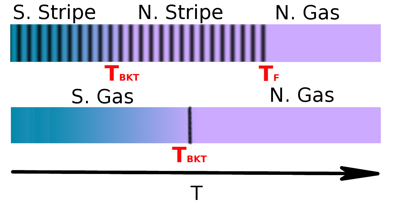
Figure 1: Phase transitions in dipolar stripes compared with the dipolar gas. N and S labels stand for normal and superfluid phases, respectively.

In a previous work Bombin et al. (2017), the superfluid properties of the different phases of a dipolar system in two dimensions were studied at zero temperature. The stripe phase, that appears for certain densities and tilting angles, was shown to exhibit the characteristics which define a supersolid state. Recently, similar results have been reported for the equivalent system in the lattice Bandyopadhyay et al. (2019). At finite temperature, there is not condensate but quasi-condensate reflected in an algebraic decay of the one-body density matrix. The transition between the superfluid (with quasi-off-diagonal long range order) and normal phases follows the Berezinskii, Kosterlitz and Thouless (BKT) theory Berezinskii (1971); Kosterlitz and Thouless (1973). This transition has been studied in many different systems such as Helium films Agnolet et al. (1989); Ceperley and Pollock (1989); Gordillo and Ceperley (1998), Coulomb layers Minnhagen (1987), and ultracold gases in pancake geometries Desbuquois et al. (2012); Ota et al. (2018); Murthy et al. (2015). It has also been shown that the BKT scenario stands even when disorder is introduced in the system Carleo et al. (2013); Maccari et al. (2018).

In this paper, we study the superfluid-to-normal phase transition in a system of two-dimensional bosonic dipoles performing first principles Path Integral Monte Carlo (PIMC) simulations. The particular case in which all the dipoles are polarized along the direction perpendicular to the plane, which constitutes the isotropic case, was already studied by Filinov et al. Filinov et al. (2010). Here, we focus on the more general case in which dipoles are polarized in an arbitrary direction, within the stability limit, and show that the BKT scaling stands despite of the anisotropy induced by the dipolar interaction. We determine the critical temperature $T_{\rm{BKT}}$ in both the gas and stripe phases. As schematically illustrated in Fig. 1, $T_{\rm{BKT}}$ for the stripe phase is smaller than $T_{\rm{BKT}}$ for the gas, at the same density. Increasing further the temperature, we observe that the normal stripes melt towards an anisotropic gas.

II Method

The system under study is composed of $N$ identical dipolar bosons of mass $m$ moving on the $XY$ plane. An external field (electric or magnetic) in the XZ plane polarizes all the dipoles along the same direction in space, forming an angle $\alpha$ with respect to the Z axis. The model Hamiltonian describing the system reads

$$H=-\frac{\hbar^{2}}{2m}\sum_{j=1}^{N}\nabla_{j}^{2}+\frac{C_{dd}}{4\pi}\sum_{i<j}^{N}\left[\frac{1-3\lambda^{2}\cos^{2}\theta_{ij}}{r_{ij}^{3}}\right]\ ,$$ (1)

with $\lambda=\sin\alpha$, and $(r_{ij},\theta_{ij})$ the polar coordinates of $\mathbf{r}_{ij}$. The strength of the dipolar interaction is encoded in the constant $C_{dd}$ and is proportional to the square of the (electric or magnetic) dipole moment of each particle. Similarly to previous works, we employ dipolar units Astrakharchik et al. (2007); Bombin et al. (2017), with the characteristic dipolar length $r_{0}=mC_{dd}/(4\pi\hbar^{2})$ and dipolar energy $\varepsilon_{0}=\hbar^{2}/(mr_{0}^{2})$ that allows for writing the Hamiltonian in dimensionless units. In the following, temperatures will be expressed also in units of $\varepsilon_{0}$. The system is stable towards collapse as long as the tilting angle $\alpha$ is smaller than the critical value $\alpha_{c}\simeq 0.61$. Our simulations are carried out in a rectangular box, with periodic boundary conditions (PBC), to correctly commensurate the stripes Bombin et al. (2017), similarly to what is made in the simulation of crystals.

For a given Hamiltonian, the PIMC method provides exact results (within some statistical noise) for the energy, structure and superfluidity of a Bose fluid or solid. It has been widely used in the past to study the BKT transition, for instance in two-dimensional liquid ⁴He Ceperley and Pollock (1989); Ceperley (1995) and in dipoles with dipolar moments perpendicular to the plane Filinov et al. (2010). Going down in temperature, and mainly close to the critical temperature, the PIMC simulation requires of a good action to reduce the number of imaginary-time steps (beads) representing each atom (polymer) to a manageable level. To this end, we use the fourth order Chin’s action Takahashi and Imada (1984a, b); Chin (2004); Chin and Chen (2002), that can be made to work effectively up to sixth order for the energy estimation by optimizing its control parameters Sakkos et al. (2009). Efficiency in the sampling of permutations is also fundamental to obtain accurate results for the one-body density matrix and superfluid densities. To get it right we use the worm algorithm, that has proven its accuracy in different systems Boninsegni et al. (2006).

At odds with what happens in three-dimensional systems, the superfluid fraction performs an abrupt universal jump Nelson and Kosterlitz (1977) at the critical temperature $T_{c}$. Near $T_{c}$, the BKT theory predicts that the correlation length has an essential singularity $\xi(T)\sim e^{a/t^{1/2}}$, with $t=(T/T_{c}-1)$ and $a$ being a non-universal parameter depending on density and on the microscopic properties of the particular system under study Kosterlitz (1974). Due to the use of a finite number of particles $N$, within a finite-size box with PBC, we do not have direct access to the critical temperature in the thermodynamic limit ($T_{c}(\infty)$) but rather to an estimation $T_{c}(L)$, with $L=\sqrt{N/n}$. As usual in finite-size scaling analysis of simulations close to the critical point, one identifies $T_{c}(L)$ with the temperature that makes $\xi(T_{c}(L))=L$. Therefore, the scaling law of the critical temperature with the size of the box can be written as Filinov et al. (2010)

$$T_{c}(L)=T_{c}(\infty)+\frac{b}{\ln^{2}(L\sqrt{n})}\ ,$$ (2)

with $b$ a non-universal constant. On the other hand, the jump that the superfluid density performs at the critical temperature $T_{c}$ follows the universal relation Nelson and Kosterlitz (1977)

$$\frac{n_{s}(T_{c},L)}{n}=\frac{2mk_{B}}{\pi\hbar^{2}}\frac{T_{c}}{n}\ ,$$ (3)

with $k_{B}$ the Boltzmann constant.

III Results

III.1 Superfluid fraction

In order to determine the critical temperature at which the superfluid-to-normal phase transition occurs, we need to evaluate the superfluid density. In the PIMC method, this is done through the well known winding number estimator Pollock and Ceperley (1987),

$$\frac{n_{s}}{n}=\frac{mk_{B}T}{N\hbar^{2}}\langle\textbf{W}^{2}\rangle\ ,$$ (4)

where W is the winding number.

III.1.1 BKT scaling of the gas phase

Using the superfluid densities, calculated with the estimator (4) at different temperatures and system sizes, and taking advantage of the universal relations of equations (2) and (3), one can obtain the superfluid-to-normal critical temperature. We start studying the transition in the gas phase at different densities and tilting angles. In Fig. 2, we show our PIMC results for the superfluid fraction $n_{s}/n$ at a density $nr_{0}^{2}=25$. In the left panel of this figure, we show our results for a tilting angle $\alpha=0.6$, close to the border of stability of the gas at zero temperature Macia et al. (2014). The critical temperature for a given system size $T_{c}(L)$ is determined as the crossing point between the universal BKT jump of Eq. (3) and the superfluid density for that system size. On the right panel of the same figure, we show how the scaling (2) is used to obtain the critical temperature in the thermodynamic limit. The analysis for different values of the tilting angle $\alpha=0$, $0.2$, $0.4$, and $0.6$ reveals that the BKT scaling stands when anisotropy is present in the system.

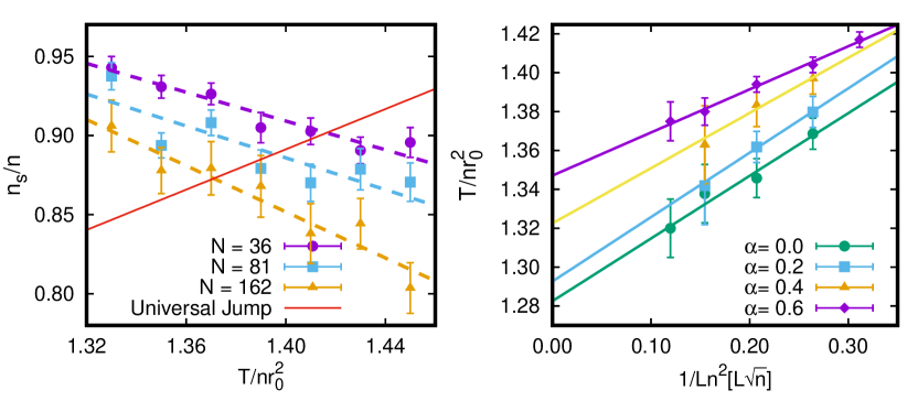
Figure 2: Left panel: superfluid fraction as a function of temperature for different system sizes at density $nr_{0}^{2}=25$ and tilt angle $\alpha=0.6$. Points are MC results, dashed lines are linear fits to PIMC data and the solid line is the universal jump of Eq. (3). The crossing points between the lines and the universal jump give the critical temperatures $T_{C}(L)$. Right panel: scaling of the critical Temperature $T_{c}(L)$ with the system size, as given by Eq. (2), at the same density and for different polarization angles. Points are PIMC data and solid lines are linear fits.

Our results for $\alpha=0$, corresponding to the isotropic gas, reproduce the PIMC estimations obtained by Filinov et al. Filinov et al. (2010). In that work, it was found a non-monotonic behavior of the critical temperature as a function of the density Filinov et al. (2010). The critical temperature, in units of density $T_{c}/nr_{0}^{2}$, increases at low densities and, above a characteristic value ($1<nr_{0}^{2}<4$), the behavior is the opposite. Filinov et al. Filinov et al. (2010) attribute this change to the appearance of the roton in the quasi-particle spectrum, which is observed to emerge around $nr_{0}^{2}=1$ Mazzanti et al. (2009); Filinov et al. (2010); Astrakharchik et al. (2007). We have studied how the tilting angle ($\alpha>0$) influences this behavior by calculating $T_{c}$ at low ($nr_{0}^{2}=0.01$) and high ($nr_{0}^{2}=25$) densities, as shown in Table 1. The behavior of $T_{c}/nr_{0}^{2}$ with the tilting angle is the opposite for densities $0.01$ and $25$: increasing $\alpha$ reduces (increases) the critical temperature at low (high) density. In both cases, though, the growth of $\alpha$ translates into an effective reduction of the interaction strength since the $s$-wave scattering length for a given tilting angle is well approximated by Macia et al. (2011),

$$a_{s}(\lambda)\simeq e^{2\gamma}\left(1-\frac{3\lambda^{2}}{2}\right)\ ,$$ (5)

with gamma the Euler’s Gamma constant. According to Eq. (5), the scattering length for dipolar interaction decreases when $\alpha$ increases. In agreement with the isotropic case Filinov et al. (2010), the effective reduction of the interaction strength lowers $T_{c}$ at low densities, where the excitation spectrum is phononic, but increases it at high densities, when rotons dominate.

Gas Phase
$nr_{0}^{2}$	$\alpha$	$T_{c}/nr_{0}^{2}$ $[\varepsilon_{0}]$	$n_{s}/n(T_{c})$	$nr_{0}^{2}$	$\alpha$	$T_{c}/nr_{0}^{2}$ $[\varepsilon_{0}]$	$n_{s}/n(T_{c})$
0.01	0.0	1.316(6)	0.838(4)	25	0.0	1.282(8)	0.816(6)
0.01	0.2	1.317(3)	0.838(6)	25	0.2	1.292(5)	0.823(4)
0.01	0.4	1.29(11)	0.821(6)	25	0.4	1.322(1)	0.842(3)
0.01	0.6	1.263(13)	0.804(8)	25	0.6	1.347(3)	0.858(2)
128	0.4	1.04(4)	0.66(3)	256	0.4	0.82(3)	0.52(2)
Stripe Phase
$nr_{0}^{2}$	$\alpha$	$T_{c}/nr_{0}^{2}$ $[\varepsilon_{0}]$	$n_{s}/n(T_{c})$	$nr_{0}^{2}$	$\alpha$	$T_{c}/nr_{0}^{2}$ $[\varepsilon_{0}]$	$n_{s}/n(T_{c})$
128	0.6	0.60(7)	0.38(4)	256	0.6	0.49(4)	0.31(3)

Table 1: BKT critical temperatures (in dipolar units) for different values of the density $nr_{0}^{2}$ and tilting angle $\alpha$, in both the gas and stripe phases. The superfluid fraction at the critical temperature is evaluated through Eq. (3). Figures in parenthesis are the estimated errors.

III.1.2 BKT scaling of the stripe phase

The stripe phase is of particular relevance in our study since it has been reported to be superfluid in the zero-temperature limit Bombin et al. (2017). The simultaneous existence of spatial long-range order (in all but one direction of the space) and off-diagonal long-range order makes this phase to be close to the pursued supersolid state of matter. A relevant issue in this discussion is whether the BKT scaling, that we have shown to hold for the anisotropic gas, stands also for the stripe phase. In Fig. 3, we show PIMC results for the superfluid fraction at a density $nr_{0}^{2}=256$ and tilting angle $\alpha=0.6$ where the stripe phase is stable Bombin et al. (2017). In the left panel, we show the behavior of the superfluid fraction as a function of temperature and for different number of particles in the simulation box. As in the gas phase, the crossing of this lines with the universal jump law of Eq. (3) allows us to extract the critical temperature for a given system size $T_{c}(L)$. In the right panel, we compare the scaling of these critical temperatures for the stripe phase with the ones obtained for the same density but at a smaller tilting angle $\alpha=0.4$ where the gas phase is the stable one. As one can see, the BKT scaling holds in both cases, and thus one can apply it to estimate the critical temperature in the thermodynamic limit.

One could think that the stripe phase is composed of quasi-one-dimensional channels, which dominate the superfluid signal, in such a way that the superfluidity in stripes follow the one-dimensional scaling law instead of the BKT one. In the next section we show that this is not the case, and thus only the BKT scenario is plausible with our results (see section III.1.3).

For temperatures lower than $T_{c}$, the superfluid fraction shows a plateau around a value which is in agreement with the zero-temperature result derived previously using the diffusion Monte Carlo method Bombin et al. (2017), $\left[\frac{n_{s}}{n}\right]_{\alpha=0.6}^{nr_{0}^{2}=256}=0.54(5)$.

In Table 1, we report the results for the critical temperature and superfluid fraction at $T_{c}$ of the stripe phase with $\alpha=0.6$ and densities $nr_{0}^{2}=128$ and $256$. By increasing the density, the critical temperature in the stripe phase decreases in a similar form to what has been previously obtained for the gas at high density. However, if the tilting angle increases, at fixed density, and crosses from the gas to the stripe phase both the superfluid fraction and the critical temperature decrease (see for instance data at $nr_{0}^{2}=128$ in Table 1). In other words, superfluidity in stripes is thermally more fragile than in the gas phase. The winding number estimator for superfluidity (4) can be split into the $X$ and $Y$ directions corresponding to the stripe orientation and its perpendicular one, respectively. At $T_{c}$, the superfluid fraction in the $Y$ direction for a finite $N$ value is $<5$% and decreases with $T$ faster than the one along the stripe direction. As it was observed previously Bombin et al. (2017), the superfluidity across the stripes depends strongly on the tilting angle, keeping the density fixed, reaching values $\sim 100$% close to the gas-stripe phase transition line but decreasing fast when entering the deep stripe region.

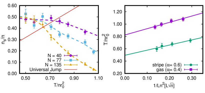
Figure 3: Left panel: superfluid fraction as a function of the temperature for different system sizes, at density $nr_{0}^{2}=256$ and tilting angle $\alpha=0.6$, corresponding to the stripe phase. Points are PIMC results, dashed lines are guides to the eye, and the solid line is the universal jump (3). Right panel: scaling of the critical temperature $T_{c}(L)$ with the system size, as given by Eq. (2), at the same density and for two tilting angles: $\alpha=0.4$ (gas) and $0.6$ (stripe). Points are PIMC data and solid lines are linear fits.

III.1.3 Non Luttinger Liquid behaviour of the stripe phase.

One may wonder if the stripe phase at finite temperature might be considered as an ensemble of one-dimensional systems. If this were the case, our data should accommodate to the predictions of the Luttinger Liquid (LL) theory. Although one-dimensional systems do not show superfluidity in the thermodynamic limit, one can still see a non-zero superfluid fraction in a finite system of length $L$. For a one-dimensional liquid, described by Luttinger theory, the superfluid fraction for a Galilean invariant system is predicted to scale with the system size as Vranješ Markić et al. (2018)

$$\frac{n_{s}}{n}=\frac{\gamma}{4}\frac{\left.|\Theta_{3}^{\prime\prime}(0,e^{-\gamma/2})\right|}{\Theta_{3}(0,e^{-\gamma/2})}$$ (6)

where $\Theta_{3}(z,q)$ is the Theta function, $\Theta_{3}^{\prime\prime}(z,q)=d^{2}\Theta_{3}(z,q)/dz^{2}$, and $\gamma=\frac{mk_{B}TL}{\hbar^{2}n_{l}}$ with $n_{l}$ the linear density.

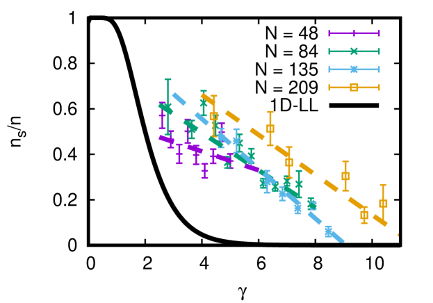
Figure 4: Superfluid fraction of the stripe phase for different number of particles as a function of the scaling parameter of Luttinger theory $\gamma$ for density $nr_{0}^{2}=128$ and tilting angle $\alpha=0.6$. Solid black line corresponds to the Luttinger liquid prediction of Eq. (6). As it can be seen, there is not collapse of the data to a single line.

In Fig. 4, we show that the data for the stripe phase ($nr_{0}^{2}=128$ and $\alpha=0.6$) do not collapse to a single line when doing the scaling with $\gamma$, with a lineal density $n_{l}=14.6(3)$ obtained from $n_{l}=N/(LN_{s})$ with $N_{s}$ the number of stripes in the simulation box containing $N$ particles. In the same figure we show the prediction of the Luttinger Liquid theory (black line), whose comparison with our results hints that the superfluid signal in the stripes is more robust against system size and temperature (encoded in the parameter $\gamma$) than what the Luttinger theory predicts for a 1D system. Therefore, we conclude that the stripe phase of a two-dimensional dipolar system cannot be considered as an ensemble of one-dimensional Luttinger liquids. This result is in agreement with the analysis of simulation data of the one-body density matrix of the stripe phase at zero temperature Bombin et al. (2017).

III.2 The One-Body density matrix

To get a deeper insight in the supersolid properties of the stripe phase, we have calculated the one-body density matrix (OBDM),

$$n_{1}(\mathbf{r}^{\prime}_{1},\mathbf{r}_{1})=\frac{V}{Z}\int d\mathbf{r}_{2}\ldots\mathbf{r}_{N}\,\rho(\mathbf{R}^{\prime},\mathbf{R}),$$ (7)

with $\mathbf{R}=\{\mathbf{r}_{1},\mathbf{r}_{2},\ldots,\mathbf{r}_{N}\}$, $\mathbf{R}^{\prime}=\{\mathbf{r}^{\prime}_{1},\mathbf{r}_{2},\ldots,\mathbf{r}_{N}\}$, $\rho(\mathbf{R}^{\prime},\mathbf{R})$ the thermal density matrix, and $Z$ the partition function. As it is well known, in 2D systems there is a condensate fraction only in the $T=0$ limit. This condensate fraction, which means that the system has off-diagonal long-range order, is obtained from the asymptotic constant value of $n_{1}(\mathbf{r}^{\prime}_{1},\mathbf{r}_{1})$ at large distances. For $T\leq T_{c}$, $n_{1}(\mathbf{r}^{\prime}_{1},\mathbf{r}_{1})$ decays with a power law instead, pointing to what is generally termed as quasi-condensate. In contrast, for $T>T_{c}$ the decay turns out to be exponential, as it corresponds to a normal phase.

In Fig. 5, we show PIMC results for the OBDM in the stripe phase ($nr_{0}^{2}=128$, $\alpha=0.6$) at different temperatures. Below the BKT transition temperature, the long-range behavior of the OBDM is well captured with a fit of the form $n_{1}(r)\sim r^{-\eta}$. The value of the exponent $\eta$ is given by the BKT theory,

$$\eta=(mk_{B}T)/(2\pi\hbar n_{s}),$$ (8)

becoming maximal at the critical point, $\eta_{c}=1/4$. As we can see in Fig. 5, the algebraic decay of the PIMC results below $T_{c}$ reproduce the BKT prediction. When the stripes become normal, the OBDM changes dramatically and we clearly see an exponential decay.

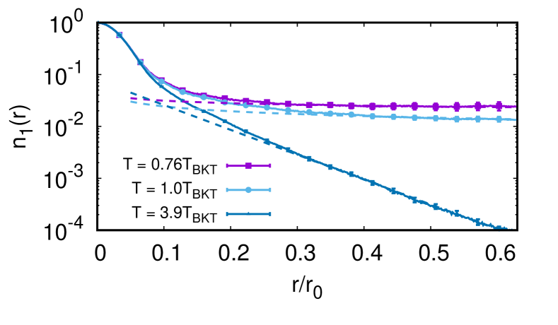
Figure 5: One-body density matrix of the stripe phase ($nr_{0}^{2}=128$ and $\alpha=0.6$) at different temperatures, above and below the transition temperature $T_{c}$. The straight lines correspond to the asymptotic behavior when $r\to\infty$.

III.3 Stripe melting

When temperature is increased beyond $T_{c}$, the stripe phase still persists as the ground state of the system, but being a normal phase (non-superfluid). Under these conditions, the static structure factor still shows a clear Bragg peak in the transverse direction ($Y$) pointing to the stability of the stripes Macia et al. (2012). Thus this is an interesting quantity if one wants to estimate, the critical temperature at which the stripe phase melts towards the gas one. To study this, we evaluate the the static structure factor for wave vectors perpendicular ($Y$) to the stripe direction ($X$),

$$S_{y}(k)=\frac{1}{NZ}\langle\hat{\rho}_{-\mathbf{k}_{y}}\hat{\rho}_{\mathbf{k}_{y}}\rangle\ ,$$ (9)

with $\hat{\rho}_{\mathbf{k}_{y}}=\sum_{i=1}^{N}e^{i\mathbf{k}_{y}\cdot\mathbf{r}_{i}}$ the density-fluctuation operator. In Fig.6, we show results of $S_{y}(k)$, for a characteristic point of the phase diagram where the system is in the stripe phase, as a function of the temperature.

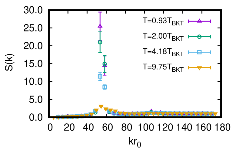
Figure 6: Evolution with the temperature of the static structure factor $S_{y}(k)$ in the stripe phase at $nr_{0}^{2}=128$ and $\alpha=0.6$.

The Bragg peak that appears at a characteristic $\mathbf{k}_{y}$ signals the periodic pattern of the stripes in their transverse direction. This large peak, which increases with the number of particles $N$ Mazzanti et al. (2009); Macia et al. (2012), is the best signature of the stripe order. When the temperature increases, the strength of the peak decreases due to the increase of the thermal motion. At the largest temperature reported in Fig.6, the Bragg peak has disappeared pointing to its melting to a gas. Notice that no equivalent peak appears at any $T$ in the $X$ direction.

However, the localization decreases progressively with $T$ until we observe their melting at a temperature $T/\simeq 10\,T_{\textsc{BKT}}$

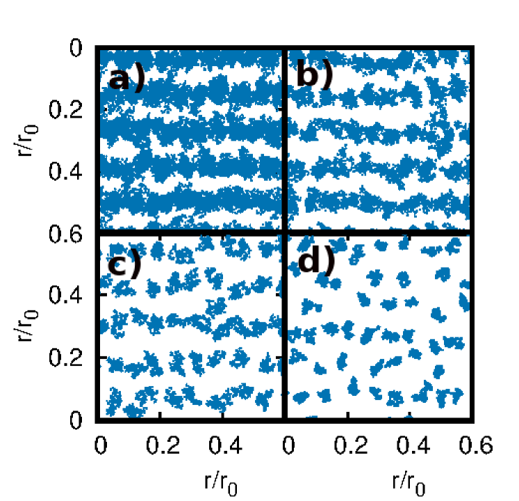
Figure 7: Snapshots of the PIMC simulations of the stripe phase for increasing temperatures at $nr_{0}^{2}=128$ and $\alpha=0.6$. The temperature $T$ increases from a) to d) panels. The values of $T$ are the same than in Fig. 6.

The evolution of the stripe structure can also be qualitatively analyzed by looking at the spatial distribution of particles in the PIMC simulation. In Fig. 7, we show snapshots to show this evolution with increasing $T$. In the PIMC framework, each particle is represented by a polymer with an averaged size proportional to its quantum delocalization. At temperatures below $T_{c}$, one can see from the snapshots that there are paths connecting the different linear structures (stripes); when these crossing paths are of the length of the simulation box there is a nonzero winding number in that direction and the superfluid fraction is finite. In the second frame of Fig. 7, this transverse paths have nearly disappeared and also in the $X$ direction the interconnections are not very abundant. In the third frame, we still observe the characteristic order of stripes but dislocations between the different lines starts to be apparent. This effect has been deeply studied in Refs. Wu et al. (2016); Mendoza-Coto et al. (2017) and now our microscopic simulations confirm these predictions. Finally, the last frame corresponds to a temperature where the stripe structure is no more present because it has melted to a (normal) gas.

IV Conclusions

In conclusion, we have carried out a complete study of the BKT transition in anisotropic 2D systems of quantum dipoles. Using the BKT theory we have estimated the superfluid-to-normal phase transition critical temperature at different densities and tilting angles. At fixed density, and increasing the tilting angle, we observe the transition from a gas to a stripe phase with a decrease on the critical temperature in the stripe case. In spite of this reduction, which makes the supersolid phase of stripes less stable against thermal fluctuations than the gas, the superfluid signal is clear below $T_{c}$. The long-range behavior of the OBDM is also consistent with the BKT prediction. Interestingly, our PIMC results on the superfluid fraction shows that its value in the transverse direction is still finite but small ($<5$%) close to $T_{c}$ and that at lower temperatures, and mainly close to the transition line to the gas, its value is much larger, almost $100$%. This result is qualitatively similar to recent experiments in which a dipolar droplet system, arranged in a quasi-one-dimensional array, has shown superfluid signatures across the drops Tanzi et al. (2019a); Chomaz et al. (2019); Böttcher et al. (2019). Regarding two-dimensional dipolar systems, similar predictions about the existence of a superfluid stripe phase have been recently reported for the equivalent system in the lattice Bandyopadhyay et al. (2019). Therefore, the quantum dipolar phases seem now the best suited candidates for the realization of the pursued supersolid state of matter. Finally, it is also worth mentioning that a superfluid stripe phase has been studied in the Hubbard model with an isotropic long-range interaction. In this case, the rotational symmetry is broken spontaneously by the interplay between the long-range character of the inter-particle interaction considered with the lattice, that forces the atoms to occupy certain lattice positions in order to minimize the energy Masella et al. (2019).