Deep motion estimation for parallel inter-frame prediction in video compression

Abstract

Standard video codecs rely on optical flow to guide inter-frame prediction: pixels from reference frames are moved via motion vectors to predict target video frames. We propose to learn binary motion codes that are encoded based on an input video sequence. These codes are not limited to 2D translations, but can capture complex motion (warping, rotation and occlusion). Our motion codes are learned as part of a single neural network which also learns to compress and decode them. This approach supports parallel video frame decoding instead of the sequential motion estimation and compensation of flow-based methods. We also introduce 3D dynamic bit assignment to adapt to object displacements caused by motion, yielding additional bit savings. By replacing the optical flow-based block-motion algorithms found in an existing video codec with our learned inter-frame prediction model, our approach outperforms the standard H.264 and H.265 video codecs across at low bitrates.

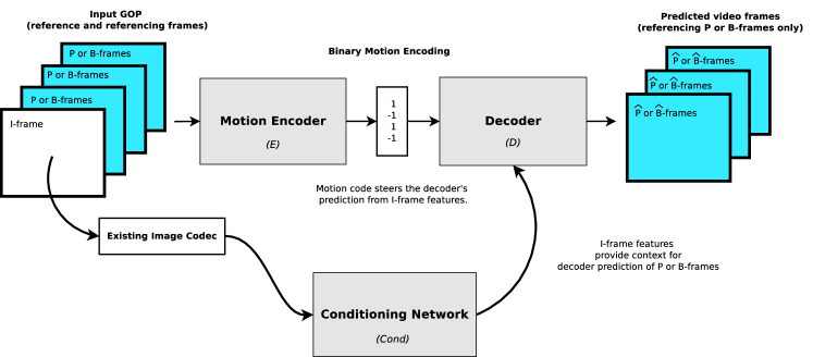
Figure 1: Video prediction network architectural overview. A learned binary motion encoding either guides the extrapolation of P-frames (Predicted-frames) from past I-frames (Intra-frame) or the interpolation of B-frames (Bi-directional-frame) from bounding past and future I-frames. Reference I-frames are coded and decoded independently with an existing image codec.

1 Introduction

Video is predicted to make up 82% of Internet traffic by the year 2022 [1]. Advancing video compression is necessary to curb high bitrates and ease bandwidth consumption. To this end, learnable deep neural networks are emerging as likely successors to hand-tuned standard video codecs [2, 3]. Inspired by recent work in binary image inpainting [4], we propose to learn binary motion codes for parallel video frame prediction. Our goal here is to show how this new parallel prediction strategy can replace the sequential flow-based methods used by existing video codecs to improve their compression efficiency.

Standard video codecs, such as H.264 [5] and H.265 [6], take advantage of the spatial and temporal redundancies in videos to aid compression. They assign video frames into one of three groups [7]: I-frames, or ‘intra-frames’, are compressed independently from surrounding frames by means of an image codec; P-frames are ‘predicted-frames’ extrapolated from past frames; and B-frames are ‘bi-directionally’ interpolated from bounding past and future frames. The compressed I-frames are transmitted directly, while the extrapolation and interpolation of P-frames and B-frames are achieved via the transmission of highly compressible optical flow vectors [8]. These motion vectors (MVs) convey motion by specifying the movement of pixels from one frame to another.

Dense optical flow [9] produces too many MVs for efficient compression (one per pixel location). Consequently, standard video codecs resort to block-based motion estimation and compensation techniques [5, 6, 10]. This entails partitioning video frames into patches called macroblocks. In the motion estimation step, each macroblock in the current frame is related to the location of the most similar macroblock in a past or future reference frame by means of an MV which contains its displacement in the $x$ and $y$ directions. Searching for representative macroblocks in the reference frame is computationally expensive and numerous search algorithms have been proposed to help speed up this process [11, 12, 13, 14, 15]. After the transmission of a reference I-frame, only MVs need be transmitted to motion-compensate macroblocks in the I-frame and form predictions of the subsequent frames within a video sequence. Standard image compression is used to encode the residuals (differences) between the vector-based motion predictions and the original video frames to improve reconstruction quality.

Block-based motion prediction, although effective, is prone to block artefacts and only allows for sequential decoding [16]. Furthermore, these algorithms suffer from hand-tuned parameterisation and lack the ability to undergo joint optimisation with the rest of a video compression system. We present a deep learning approach to video frame prediction that can be optimised end-to-end as part of a larger video compression system. Given I-frame context, our model is also able to decode P-frames or B-frames in parallel without the additional overhead of motion-estimation search.

Our approach is illustrated at a high level in Figure 1. Video interpolation aims to predict a set of unseen intermediate frames from a pair of bordering reference frames. Video extrapolation, on the other hand, forecasts unobserved video frames based on those that have occurred in the past. In our approach, an encoder $E$ learns how to produce a binary motion encoding, shown in the middle of the figure, with binarisation performed directly within the neural network. The resulting learned binary motion code is subsequently used to guide the extrapolation of P-frames conditioned on a past I-frame, or the interpolation of B-frames conditioned on bounding past and future I-frames. Interpolation or extrapolation is performed by the decoder $D$ and the conditioning is indicated through the ‘Cond’ block in the figure, which extracts features from I-frames that have been compressed and decompressed independently by an existing image codec. We therefore view the decoding of P-frames or B-frames in video compression as motion guided interpolation or extrapolation, where a low dimensional learned binary motion code helps direct prediction from I-frames.

1.1 Related Work

In work interested purely in prediction (without compressing), deep learning has been shown to produce high quality video frame interpolations [17, 18, 19, 20, 21, 22, 23, 24] and extrapolations [25, 26, 27, 28] for small time-steps. Typically, unseen video frames are predicted solely based on the reference frame [18, 21, 22]. For predicting unseen frames over longer time-spans (as would be the case if we were interested in video compression), additional information is required.

In video compression, we do not need to rely solely on the reference frame content: we can estimate the motion from the actual unseen video frames, compress these motion encodings, and then transmit this together with the compressed versions of the reference frames. This extra motion information can enable video frame prediction over extended timespans [29]. Based on this idea, deep learning has recently been applied to video compression, producing models capable of outperforming standard video codecs (H.264, H.265) at certain bit allocations [2, 3, 29, 30, 31, 32]. These models combine state-of-the-art image compression, flow prediction and entropy coding networks to produce end-to-end optimisable video compression systems. Despite their success, whole systems are evaluated as a single unit, making it difficult to discern to what extent each individual component outperforms its more conventional standard implementation. In this work, we focus specifically on motion compression for video prediction—we consider P- and B-frame prediction in isolation, decoupled from all other compression components.

In [29], video frames are hierarchically interpolated by warping input reference frame features with standard block-MVs, while discrete representations of motion are learned by encoding optical flow patterns in [2, 3]. Optical flow vectors describe how pixels in a video frame should be moved over time to best estimate true object and camera motion [33]. It is effective at modeling translational motion, but fails to capture more complex transformations such as rotation, warping, occlusion and changes in lighting [8]. [2, 3, 29] address this by jointly compressing the residuals produced after flow compensation. In this paper, rather than using optical flow, we show that it is possible to learn compact encodings that are representative of complex motion directly from a video sequence. More specifically, we train an encoder network to produce learned binary motion codes which guide the prediction of P-frames and B-frames from I-frame context at the decoder. Experiments show that the complex motion contained in our binary motion codes outperforms that of conventional optical flow. The codes produced by our network could, therefore, provide an alternate means of motion conditioning for applications that are currently reliant on optical flow-based methods [2, 3, 29, 34].

Different spatial and temporal locations in a video sequence are not necessarily equally complex. In image compression, it has been shown that compression rates can be improved by varying bitrates such that less complex image regions are assigned fewer bits [35, 36, 37, 38, 39]. Varying the bitrate temporally in accordance to complexity of motion is equally important in video compression [5, 6, 10]. Most videos contain still segments interspersed with sequences depicting rapid motion. A model with access to reference frame context at its decoder should learn to encode very little information for still video segments and allocate the bulk of its bits to intervals containing a high degree of motion. In [2, 40] recurrence is used to sequentially maintain state information across time such that previously decoded information need not be re-encoded. We, on the other hand, extend the 2D content-weighted image compression technique in [37] to three dimensions and present parallelised P-frame and B-frame video compression models that learn to vary bitrate both spatially and temporally. Experiments show how our approach to 3D dynamic bit assignment substantially reduces the bitrate of a motion encoding model without adversely affecting its reconstruction quality.

1.2 Contributions

We proceed as follows. First we give a detailed description of our P-frame and B-frame compression architectures. We then formulate our approach to 3D content-aware bit weighting and demonstrate its applicability to bitrate optimisation. Finally, compression efficiency is evaluated in terms of various video quality metrics (PSNR, SSIM, VMAF and EPE). We demonstrate that our models’ P-frame and B-frame predictions outperform those of the block-motion prediction algorithms employed by standard video codecs such as H.264 and H.265. Additional experiments are carried out to determine the impact of an optical flow-based loss term and if multi-scale convolutions result in richer motion sampling. We find that including multi-scale convolutions in our encoder architecture slightly improves the quality of our model’s video frame predictions. On the other hand, limiting our model to learning pixel-wise translational motion with a flow loss term worsens its prediction quality. This indicates that we are able to learn more representative motion than conventional optical flow. A full implementation of the code developed as part of this work is made available online: DeepVideo.

2 Video Frame Prediction Architecture

2.1 Architectural Overview

Figure 1 illustrates our approach to P-frame and B-frame prediction. The neural network encoder $E$ compresses and binarises the motion occurring in a Group Of Pictures (GOP): a video segment containing designated reference (I) and referencing (P or B) frames. Binarisation via thresholding is non-differentiable. To perform this operation directly within a neural network, we therefore resort to the stochastic binarisation function presented in [41]: during training, each encoder output, which lies within $(-1,1)$, is made to take one of two distinct values in the set $\{-1,1\}$ by adding uniform quantisation noise. This allows for a straight through estimate [42] of gradients, i.e. gradients flow through the binarisation layer unchanged. At the decoder $D$, I-frame features extracted by the conditioning network ‘Cond’ are transformed based on the information held in the binarised motion encoding to predict the P or B referencing frames. Note that ‘Cond’ is not responsible for I-frame compression: this is done by an existing image codec.

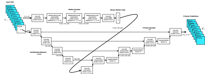
Figure 2: The P-frame prediction network (P-FrameNet) used to extrapolate video frames from a past I-frame.

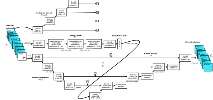
Figure 3: The B-frame prediction network (B-FrameNet) used to bi-directionally interpolate video frames from bounding past and future I-frames.

2.2 P-frame and B-frame Prediction Networks

Figures 2 and 3 illustrate our P-frame and B-frame prediction networks in greater detail. Equations (1) and (2) summarise the P-frame and B-frame prediction processes depicted in Figures 2 and 3, respectively.

$$\widehat{P_{1,\ldots,t}}=D\left(E(I_{0},P_{1,\ldots,t}),\textrm{Cond}(I_{0})\right)$$ (1)

$$\widehat{B_{1,\ldots,t}}=D\left(E(I_{0},B_{1,\ldots,t},I_{t+1}),\textrm{Cond}_{0}(I_{0}),\textrm{Cond}_{t}(I_{t+1})\right)$$ (2)

The decoder $D(\cdot)$ uses context derived from reference frames $I$ by the conditioning network $\textrm{Cond}(\cdot)$ to predict a sequence of $t-1$ frames, $P_{1,\ldots,t}$ or $B_{1,\ldots,t}$. The prediction process is supervised by a binarised motion encoding, $E(\cdot)$, of the original GOP sequence. Because the encoder always compresses the input GOP’s width, height and time axes by a factor of 8, P-FrameNet and B-FrameNet’s bitrate is determined by the number of output channels we set in the final encoder layer, $C_{\textrm{bnd}}$. We denote predicted video-frames as either $P$ or $B$, depending on whether the decoder performs motion guided extrapolation or interpolation. The decoder performs extrapolation, Figure 2, when conditioned on a single I-frame, $I_{0}$, and interpolation, Figure 3, when conditioned on a pair of bounding I-frames, $I_{0}$ and $I_{t+1}$. During training we use a $L_{2}$ reconstruction loss:

$$L_{R}=\lvert\lvert{B-\hat{B}}\rvert\rvert^{2}\quad\text{or}\quad\lvert\lvert{P-\hat{P}}\rvert\rvert^{2},$$ (3)

Throughout training we give $D(\cdot)$ access to the original I-frame content, but at test time $I_{0}$ and $I_{t+1}$ are encoded and decoded independently by an existing image codec.

Motion in video often occurs at different scales. To account for this, we implement 3D multi-scale convolutional layers [43, 44] in our encoder network as a lightweight substitute for deep pyramidal decomposition [25, 45]. Each multi-scale convolution combines filters with different dilation factors for more diverse motion sampling across a range of spatial and temporal scales, and can be seen as a type of learned scale invariant feature transform (SIFT) [46]. In Section 4.2 we demonstrate how the inclusion of multi-scale convolutions consistently improves video frame prediction quality. As shown in Figures 2 and 3, manifold layers from the conditioning network ‘Cond’ are joined to the decoder $D$ in a fashion reminiscent of the U-Net [47] architecture, prevalent in previous video interpolation work [18, 21]. I-frame conditioning at the decoder enables P-FrameNet and B-FrameNet to learn motion compensation (how to transform I-frame content) instead of just compressing input P- and B-frames directly. The experiment in Section 4.1 shows that the binary motion codes learnt through I-frame conditioning are more easily compressible than raw video frames. Upscaling at the decoder is accomplished via pixel-shuffling [48], an efficient alternative to transposed convolutions. Scene changes and motion complexity often dictate GOP length selection in standard codecs [8]. Our designs are, therefore, fully convolutional to ensure that they are able to accommodate a diverse range of input frame-sizes and dynamic GOP lengths.

2.3 3D Dynamic Bit Assignment

In order to vary the bitrate of our binary motion codes, we leverage [37]’s approach to content-weighted image compression and learn to vary bitrate across an extra dimension: time. Video regions that are smooth and predominantly stationary are easier to compress than those containing rich texture and rapid motion. An ideal motion compression model should, therefore, actively adapt its bitrate according to fluctuations in video complexity by assigning fewer bits to simplistic video regions and vice versa. As it stands, our encoder architecture allocates a fixed number of bits to each spatio-temporal location in its code-space, specified by $C_{\textrm{bnd}}$, the number of channels in its binarisation layer. Based on [37], we learn a 3D bit-distribution-map, $B_{\textrm{map}}$, that determines how many bit channels are allocated to our binary motion encoding per point in space-time.

Figure 4 illustrates the key stages in our approach to 3D dynamic bit assignment. First we learn $B_{\textrm{map}}$, shown at (i) in the figure, from the input GOP by passing features extracted by the penultimate encoder layer through a 3D convolutional network. $B_{\textrm{map}}$ is a single-channel feature map whose values fall in the range $(0,1)$ and whose spatial and temporal size is the same as the binary motion code produced by the encoder, represented by the blue cubes at (ii). While in the figures thus far we have indicated the serialised motion encoding with a box of $-1$ and $1$s, the cubes at (ii) in this figure indicate the individual learned MVs for each video frame over its width and height (these are serialised later, as explained below). The lighter regions in $B_{\textrm{map}}$ are higher valued and identify video regions that should be allocated more bits (channels). Following [37], we portion the available $C_{\textrm{bnd}}$ bits produced for each video frame by the encoder into $L$ groups each containing $\frac{C_{\textrm{bnd}}}{L}$ bits. With $\lfloor\cdot\rfloor$ denoting the mathematical floor operator, each element, $b_{t,h,w}$, in $B_{\textrm{map}}$ is quantised to one of $L$ integer levels,

$$Q_{L}(b_{t,h,w})=\lfloor Lb_{t,h,w}\rfloor$$ (4)

to decide how many bit levels need to be retained per point in space-time. To avoid allocating non-integer bit numbers we require that $C_{\textrm{bnd}}$ be cleanly divisible by $L$ and $L\leq C_{\textrm{bnd}}$. Guided by $Q_{L}(B_{\textrm{map}})$ at (iii), we populate a mask $M$, shown at (iv), that zeros-out unnecessary bit channels produced by the encoder at (ii):

$$m_{c,t,h,w}=\begin{cases}1,&\text{if $c\leq\frac{C_{\textrm{bnd}}}{L}Q_{L}(b_{t,h,w})$}\\ 0,&\text{otherwise}\end{cases}$$ (5)

The cubes at (v) shows how masked bits (zeros) are cropped-out prior to the transmission of the serialised motion bitstream. Zeros are reinstated at the decoder by zero-padding each channel to $C_{\textrm{bnd}}$ (the maximum bit-length). After multiplication by $M$ and zero-cropping, the number of bits transmitted per point in space-time is reduced from $C_{\textrm{bnd}}$ to $\frac{C_{\textrm{bnd}}}{L}Q_{L}(b_{t,h,w})$. In order for the decoder to reshape the serial bitstream correctly, a binarised version of $Q_{L}(B_{\textrm{map}})$ is sent separately as additional overhead at (vi). The integer values in $Q_{L}(B_{\textrm{map}})$ are binarised using base-2 expansion [49] for transmission.

Realising that our serial bit-count is proportional to the summation over $B_{\textrm{map}}$, we can use an additional loss term,

$$L_{B}=\sum_{t,h,w}b_{t,h,w}$$ (6)

to drive down our model’s bitrate during training [37]. $L_{B}$ penalises bitrates above zero. This prevents assigning bits to stationary video regions that can be deduced from I-frame context alone.

Both the mask formation, (iv), and quantisation functions, (iii), in equations (4) and (5) are non-differentiable. Luckily, using straight through estimation [37, 42] again, the gradient of $M$ with respect to $b_{t,h,w}$ can be approximated by,

$$\frac{\partial m_{c,t,h,w}}{\partial b_{t,h,w}}=\begin{cases}L,&\text{if $Lb_{t,h,w}-1\leq\lceil\frac{cL}{C_{\textrm{bnd}}}\rceil\leq Lb_{t,h,w}+2$}\\ 0,&\text{otherwise}\end{cases}$$ (7)

We show the benefit of this 3D dynamic bit assignment approach experimentally in Section 4.5.

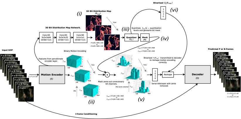
Figure 4: 3D dynamic bit assignment incorporated into a video frame prediction model to vary its bit allocations across space-time. In this figure the motion encoding bit-space is represented in its true multi-dimensional form by blue blocks. $B_{\textrm{map}}$, indicated by (i) in the figure, is used to generate a mask $M$ at (iv) that crops out unnecessary bits at (v).

2.4 Optical Flow Loss

We deploy the setup shown in Figure 5 to determine if including an explicit additional optical flow based loss term leads to improved motion compression. The optical flow between two video frames is defined by a 2D vector field that relates the movement of pixels from the one frame to the other [8]. We denote the dense (per-pixel) optical flow for each consecutive pair of frames in the input GOP as $\vec{V_{g}}$: the ground truth flow, indicated at (i) in the figure. As shown at (ii), $\vec{V_{p}}$ represents the flow vectors derived from the frames predicted by our motion compression network. A host of techniques can be used to calculate $\vec{V_{g}}$ and $\vec{V_{p}}$, including differential [9], phase [50] and energy [33] based methods, or more recent deep learning approaches [51, 52, 53, 54, 55]. In this work, we use LiteFlowNet [55], a state-of-the-art deep flow estimation model. LiteFlowNet’s weights are pre-trained on the MPI Sintel dataset [56] and frozen when training our video compression models. We experiment with the optical flow losses defined by the Euclidean distance between the ground truth and predicted flow vectors called the end-point-error (EPE),

$$L_{\textrm{EPE}}=\sqrt{\lvert\lvert{\vec{V_{g}}-\vec{V_{p}}}\rvert\rvert^{2}},$$ (8)

and cosine similarity,

$$L_{\textrm{cosine}}=1-\frac{\vec{V_{g}}\cdot\vec{V_{p}}}{\|\vec{V_{g}}\|\ \|\vec{V_{p}}\|}.$$ (9)

$L_{\textrm{cosine}}$ differs from $L_{\textrm{EPE}}$ in that it only penalises directional deviations between the ground-truth and predicted flow vectors as disregarding differences in magnitude may provide beneficial regularisation. We normalise the $x$ and $y$ components of the flow vectors in $\vec{V_{g}}$ and $\vec{V_{p}}$ by the width and height of the input video frames to avoid directional biasing. We investigate the consequences of adding these optical flow loss terms in Section 4.3.

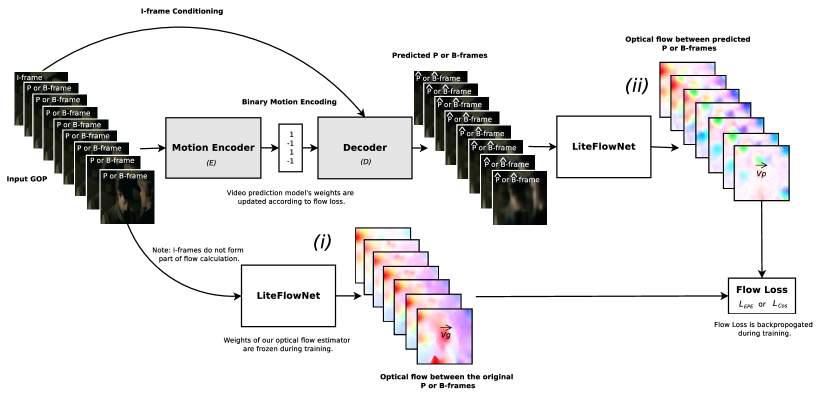
Figure 5: Setup used to train a video frame prediction network with an optical flow based loss term. We use LiteFlowNet [55] to calculate and compare the optical flow of the input and predicted video frames. LiteFlowNet’s weights are fixed when optimising our video frame prediction models.

3 Experimental Setup

3.1 Data and Training Procedure

The P-frame and B-frame prediction networks in Figures 2 and 3 are trained on the Hollywood dataset [57]. This dataset contains 475 AVI movie clips from a wide range of classic films. The average clip length in our training corpus is around 5 seconds. Prior to training we transcode each clip with the H.264 [5] codec to ensure NVIDIA Video Loader (NVVL) data loader compatibility [58, 59]. We split this dataset into training and validation sets containing 435 and 40 clips, respectively. To avoid learning compression artefacts introduced by H.264, we train our models on resized $64\times 64$ pixel video frames. During training we randomly crop a GOP from each clip, so although our dataset only contains 435 videos, our models are exposed to substantially more data. The GOPs used for validation are cropped from the start of each video in the validation set to ensure that the validation losses used for early stopping are directly comparable across epochs. GOP length is set to 18 for B-FrameNet and 17 for P-FrameNet. In both cases our models are trained to predict 16 video frames using the reconstruction loss in equation (3). Input video clips are grouped into batches of 3 and their pixel values are normalised to fall in the range $(-1,1)$. The training process spans 150 epochs and utilises Adam optimisation [60]. The initial learning rate is set to 0.0001 and decayed by a factor of 2 at epochs 30, 100 and 140. We train models with a range of bottleneck-depths $C_{\textrm{bnd}}$ to gauge performance across a range of bitrates.

3.1.1 Bitrate Optimisation

Pre-trained P-FrameNet and B-FrameNet models are trained to perform 3D dynamic bit assignment (Section 2.3) by undergoing another 150 epochs of training with the optimisation function defined by

$$L_{RB}=L_{R}+\lambda L_{B}$$ (10)

$L_{RB}$ combines the reconstruction loss $L_{R}$ in equation (3) with the loss $L_{B}$ in equation (6) that encourages low bitrates.

As done in [37], we introduce the hyperparameter $\lambda$ to control the trade-off between reconstruction quality and compression rate. Setting $\lambda=0$, zeros-out $L_{B}$, which prevents a model from learning to vary its bitrate.

3.1.2 Flow Loss

When training our models to minimise the difference between the optical flow of the input and that of the predicted frames (Section 2.4) we use the loss defined by,

$$L_{RF}=L_{R}+\alpha L_{F}$$ (11)

where $L_{F}$ is one of the the optical flow losses in equations (8) or (9) and $L_{R}$ is the distortion loss in equation (3). $\alpha$ is a weighting term used to normalise $L_{F}$ by the total number of flow vectors during training.

3.2 Evaluation

To quantify the quality of our predicted video frames we use three objective evaluation metrics: Peak Signal to Noise Ratio (PSNR), Structural SIMilarity index (SSIM) [61], and Video Multi-method Assessment Fusion (VMAF) [62]. PSNR and SSIM measure the degree to which an image reconstruction corresponds to the original image, so we calculate PSNR and SSIM for video by averaging scores across the predicted video frames. SSIM falls within $[-1,1]$ while PSNR can be any real value and is expressed in dB. Higher scores signify greater prediction quality.

We also assess our video compression with the VMAF framework developed and deployed by Netflix [62]. VMAF is a machine-learning based video quality metric trained to combine the results of various perceptual models such that its scores are more closely aligned with the human visual system than a stand-alone objective algorithm [62]. VMAF scores fall in the range $[0,100]$, with a higher score again indicating greater reconstruction quality [63].

To understand and probe different aspects of our approach, the experiments in Section 4 are carried out on videos from our validation set: the 40 videos from the Hollywood dataset [57]. In Section 5 final versions of P-FrameNet and B-FrameNet are pitted against the block-motion algorithms used in standard video codecs. This evaluation is carried out on 235 raw (‘.yuv’) video clips sampled from the Video Trace Library (VTL) [64]. Each clip is partitioned into 17-frame or 18-frame sequences depending on whether we are predicting P-frames or B-frames, such that our models always predict 16-frames. VMAF, SSIM, PSNR and EPE scores are then calculated and averaged across the reconstructed video-frames. We denote EPE as EPE (FlowNet) or EPE (Farneback) depending on whether we calculate optical flow using LiteFlowNet [55] or Farneback’s polynomial method [9]; in contrast to the other metrics, lower EPE is better.

4 Results: Ablation Experiments and Analysis

In order to probe and better understand our approach through ablation studies and developmental experiments, we guide our analysis using the following questions.

4.1 P-frame vs. B-frame Decoder Conditioning?

We explore the benefits of conditioning our video decoder on learned features extracted from reference I-frames (Section 2.2). Table 1 compares a video autoencoder (P-FrameNet without I-frame conditioning) to P-FrameNet (single reference frame conditioning) and B-FrameNet (dual reference frame conditioning) in Figures 2 and 3, respectively. In Table 1 conditioning is shown to consistently improve the quality of the predicted frames as it allows the encoder to focus primarily on motion extraction—we learn to transform available pixel-content rather than compressing it directly.

Table 1 reaffirms that motion transforms are easier to compress than raw video content [8]. B-frame conditioning is shown to outperform its P-frame counterpart, as context from bounding reference frames allows it to learn both forward and reverse motion transformations. Unlike standard video codecs, B-FrameNet is able to predict B-frames in parallel without the extra overhead of having to transmit the order in which frames are to be decoded [6].

Table 1: Quality scores for various decoder conditioning schemes.

Conditioning	PSNR	SSIM	VMAF
None	$23.71$	$0.64$	$41.21$
P-frame	$28.25$	$0.80$	$62.31$
B-frame	$\mathbf{29.83}$	$\mathbf{0.84}$	$\mathbf{70.45}$

4.2 Do Multiscale Convolutions Learn More Representative Motion?

We experiment with incorporating the multi-scale convolutions [43] discussed in Section 2.2 in our motion encoder architecture. This provides us with a lightweight means of sampling motion at a variety of spatial and temporal scales. Table 2 compares two implementations of P-FrameNet, one with multi-scale convolutions and the other with normal convolutions in its motion encoder. Using multi-scale convolutions leads to modest but consistent improvements in the quality of the predicted frames, as indicated by higher PSNR, SSIM and VMAF scores. It also allows P-FrameNet to perform more representative motion encoding (lower EPE). Multi-scale convolutional layers are, therefore, used in our motion encoders throughout the rest of this work.

Table 2: Multis-scale vs. standard convolutional implementations of P-FrameNet.

Convolution	PSNR	SSIM	VMAF	EPE
				FlowNet	Farneback
Standard	$28.25$	$0.80$	$62.31$	$0.477$	$9.28\cdot 10^{-7}$
Multiscale	$\mathbf{28.48}$	$\mathbf{0.81}$	$\mathbf{63.90}$	$\mathbf{0.471}$	$\mathbf{9.24\cdot 10^{-7}}$

4.3 Is an Optical Flow Based Loss Beneficial?

We experiment with the EPE and cosine similarity flow losses in equations (8) and (9) in Section 2.4 to discover if an optical flow based penalty helps B-FrameNet to learn improved motion. As stated in equation (11) in Section 3.1.2, we add our chosen flow loss, $L_{F}$, to the reconstruction loss, $L_{R}$, during training. The hyperparameter $\alpha$ in equation (11) is used to weight $L_{F}$ such that the mean loss per flow vector is added to $L_{R}$.

Table 3 reveals that an additional optical flow loss term worsens the quality of B-FrameNet’s reconstructions (lower PSNR, SSIM and VMAF scores). The added loss term does, however, cause the optical flow of the predicted frames to match that of the input more closely (lower EPE). At first glance, this result seems contradictory. How can learning better motion lead to a depreciation in quality? Realising that optical flow is essentially only 2D pixel shuffling, the results in Table 3 imply that B-FrameNet is able to learn more advanced motion transforms (rotation, warping, occlusion and colour shift) when it is not limited to translational motion by a flow loss term. Informal experiments showed that increasing the weight $\alpha$ of the flow loss term in equation (11) improved the EPE but further degraded the quality of the predicted video frames.

Table 3: Influence of an additional EPE (equation (8)) or cosine (equation (9)) optical flow loss term on B-FrameNet’s performance.

Flow Loss	PSNR	SSIM	VMAF	EPE
				FlowNet	Farneback
None	$\mathbf{29.81}$	$\mathbf{0.842}$	$\mathbf{71.03}$	$0.477$	$9.21\cdot 10^{-7}$
EPE	$29.59$	$0.836$	$70.19$	$\mathbf{0.461}$	$\mathbf{9.17\cdot 10^{-7}}$
Cosine	$24.04$	$0.652$	$59.44$	$0.514$	$9.69\cdot 10^{-7}$

4.4 What are Optimal Parameters for Learning 3D Dynamic Bit Assignment?

With this experiment we try to find an optimal parameterisation of the 3D dynamic bit assignment loss $L_{RB}$ in Section 3.1.1. We tune B-FrameNet ($C_{\textrm{bnd}}=8$) with different quantisation levels $L$ in equation (4) and different values of $\lambda$ for the weight of the binary penalisation term $L_{B}$ in the overall loss $L_{RB}$ in equation (10). The learned bitrates and corresponding VMAF scores are shown in Figure 6.

Using $\lambda=0$ (no 3D dynamic bit assignment) as a point of reference, we find that setting $L$ equal to its maximum possible value, in this case the channel depth $8$, yields the best compression efficiency. $L$ controls the number of bit levels the model can choose from per point in space-time. Higher settings of $L$ gives B-FrameNet more options in deciding how many bits to allocate to different video regions, bringing about a lower bitrate on average. Setting $L$ too low, $L=2$, worsens compression as the bit-savings are not substantial enough to outweigh the cost of sending the quantised bit distribution map at (vi) in Figure 4. We see that for $L=8$ and $L=4$, setting $\lambda=0.0001$ is optimal, as it results in the greatest bit reduction without decreasing the quality of the predicted frames below that of the reference point, $\lambda=0$. Based on these results we set $\lambda=0.0001$ and $L$ equal to our encoder’s bottleneck-depth $C_{\textrm{bnd}}$ whenever optimising a system for 3D dynamic bit assignment.

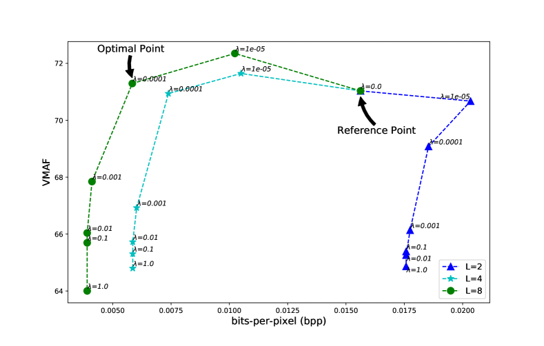
Figure 6: VMAF scores and learned bitrates produced on development data by B-FrameNet trained with different parameterisations of $L_{RB}$.

4.5 Does 3D Dynamic Bit Assignment Aid Motion Compression?

To establish whether 3D dynamic bit assignment aids compression efficiency, we train B-FrameNet to vary its bitrate across space-time (Sections 2.3 and 3.1.1). We train several instantiations of B-FrameNet with different bit channel depths, $C_{\textrm{bnd}}=\{6,8,16,32,64\}$, to assess the impact of learned dynamic bit assignment at different operating points. The compression curves in Figure 7 show that optimising a model for 3D dynamic bit assignment substantially improves its PSNR, SSIM and VMAF scores across all bitrates, even with the additional overhead of transmitting the binarised importance map, $Q_{L}(B_{\textrm{map}})$.

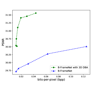
(a) PSNR

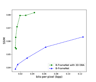
(b) SSIM

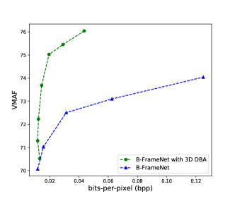
(c) VMAF

Figure 7: B-FrameNet with and without 3D dynamic bit assignment (3D DBA).

4.6 Do Spatial Bit Allocations Change Over Time?

Figure 8 plots B-FrameNet’s bit-distribution map $B_{\textrm{map}}$ for the given 26-frame input GOP. Because B-FrameNet compresses both space and time by a factor of around 8, $B_{\textrm{map}}$ consists of three distinct bit distributions—one per 8 frame interval. Higher valued regions in $B_{\textrm{map}}$ are brighter and correspond to areas encoded with more bits.

The optical flow charts in Figure 8 are plotted in the hue saturation value (HSV) colour space. The angular direction of the optical flow vectors is indicated by hue, so that vectors pointing in the same direction are coloured the same. Saturation indicates the magnitude of the vectors, so vectors with higher magnitudes (moving objects) are less transparent and are represented with more intense colours. Comparing $B_{\textrm{map}}$ to the optical flow charts in Figure 8, we notice qualitatively that more bits are assigned to regions containing moving objects (brightly coloured regions in the optical flow chart).

$B_{\textrm{map}}$’s spatial bit distribution also changes across time to compensate for object displacements caused by motion. As an aside, for video scenes containing rapid motion or multiple scene changes it may help to lessen B-FrameNet’s compression factor across time as this would yield more frequent updates to $B_{\textrm{map}}$.

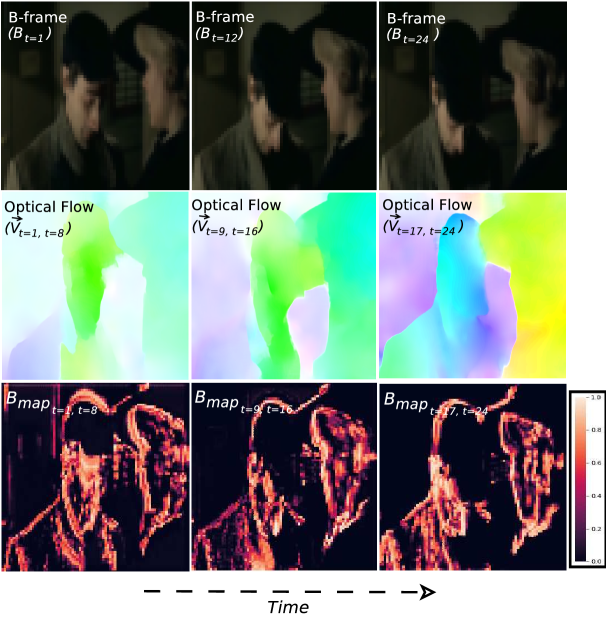
Figure 8: B-FrameNet’s bit-distribution map, $B_{\textrm{map}}$, compared to optical flow (FlowNet) and input video frames. Brighter regions in $B_{\textrm{map}}$ are allocated higher bitrates and correspond to moving objects.

5 Results: Comparing to Conventional Video Compression

We next compare our learned video compression approach to standard codecs.

5.1 Deep Motion Estimation vs. Standard Block Motion Algorithms

Block-based motion estimation involves finding motion vectors (MVs) that model the movement of macroblocks between consecutive video frames. We compare P-FrameNet and B-FrameNet, $C_{\textrm{bnd}}=8$, optimised for 3D dynamic bit assignment to several block-based motion estimation algorithms employed by standard video codecs, namely:

• Exhaustive Search (ES) [8]

• Three Step Search (TSS) [65]

• New Three Step Search (NTSS) [11]

• Simple and Efficient Search (SES) [13]

• Four Step Search (FSS) [12]

• Diamond Search (DS) [14]

• Adaptive Rood Pattern Search (ARPS) [15]

This evaluation is carried out on videos from the VTL dataset [64]. Our models are intended for video prediction only, so here we strip down the standard video codecs so that only the mechanisms used for inter-frame prediction are compared. We apply these standard algorithms to $IPPP$ GOP sequences, so that each macroblock in the currently decoded P-frame is linked to the closest matching macroblock region from the preceding frame by way of a MV that indicates its relative spatial displacement.

For transmission, we binarise each MV’s $x$ and $y$ components as well as the centre coordinates of the reference macroblock to which it points. Zero-vectors and overhead bits needed for reshaping are discounted; here we only consider bits that effect motion transformation. Searching all possible pixel locations in the reference frame for each predicted macroblock’s closest match is computationally expensive, especially for high resolution videos. Hence, the search area is typically limited to $p=7$ pixels around the predicted macroblock’s location [7]. We experiment with $\textrm{mb}=8\times 8$ and $\textrm{mb}=16\times 16$ macroblock size parameterisations of the different algorithms in Tables 4 and 5, respectively. Smaller macroblocks produce denser MVs resulting in finer motion prediction at the cost of a higher bitrate and longer execution time. In this evaluation all models and algorithms are used to predict sixteen $224\times 320$ video frames. Note that for this evaluation we assume uncompressed I-frame context is available at the decoder.

Tables 4 and 5 show that for fewer bits-per-pixel (bpp), P-FrameNet and B-FrameNet’s predictions score higher in terms of PSNR and VMAF than those produced by the block-matching algorithms. SSIM scores are comparable, but our models use at least 23% and 88% fewer bpp than the block-matching algorithms in Tables 4 and 5, respectively. P-FrameNet and B-FrameNet’s encoding and decoding time is faster than than that of all the block-based motion estimation algorithms. This speedup stems from their ability to predict frames in parallel without the need for a search-step during encoding.

Table 4: Motion compensation scores for 16 frame video prediction $(\textrm{mb}=16\times 16,p=7)$.

Model	bpp	PSNR	SSIM	VMAF	Time (sec)
ES	$0.0108$	$16.35$	$0.850$	$44.64$	$11.35$
TSS	$0.0108$	$16.37$	$0.851$	$44.81$	$1.53$
NTSS	$0.0107$	$16.34$	$0.851$	$44.76$	$1.18$
SES	$0.0068$	$15.80$	$0.846$	$40.94$	$0.96$
FSS	$0.0077$	$16.29$	$0.852$	$44.77$	$1.01$
DS	$0.0100$	$15.70$	$0.816$	$37.90$	$0.77$
ARPS	$0.0097$	$15.66$	$0.816$	$37.89$	$0.63$
P-FrameNet	$0.0052$	$28.89$	$0.829$	$65.66$	$0.28$
B-FrameNet	$\mathbf{0.0038}$	$\mathbf{30.36}$	$\mathbf{0.859}$	$\mathbf{71.19}$	$\mathbf{0.28}$

Table 5: Motion compensation scores for 16 frame video prediction $(\textrm{mb}=8\times 8,p=7)$.

Model	bpp	PSNR	SSIM	VMAF	Time (sec)
ES	$0.0582$	$19.45$	$0.901$	$62.97$	$46.32$
TSS	$0.0578$	$19.47$	$0.901$	$63.15$	$5.67$
NTSS	$0.0568$	$19.44$	$\mathbf{0.902}$	$63.17$	$4.29$
SES	$0.0396$	$18.80$	$0.893$	$57.18$	$3.71$
FSS	$0.0437$	$19.38$	$0.901$	$62.19$	$3.86$
DS	$0.0552$	$18.58$	$0.860$	$53.09$	$2.82$
ARPS	$0.0539$	$18.54$	$0.861$	$53.16$	$2.15$
P-FrameNet	$0.0052$	$28.89$	$0.829$	$65.66$	$0.28$
B-FrameNet	$\mathbf{0.0038}$	$\mathbf{30.36}$	$0.859$	$\mathbf{71.19}$	$\mathbf{0.28}$

5.2 Deep Motion Compression vs. Standard Video Codecs

In Section 5.1 we demonstrated that with fewer bits our learned binary motion codes are able to express richer motion than several block-based motion estimation algorithms. Standard video codecs improve MV compression via techniques not included in the standalone implementation of the algorithms used above. To reduce bitrate, similar MVs are grouped together and only the Motion Vector Difference (MVD) between each vector and a Motion Vector Predictor (MVP) is transmitted [66]. MVD values are normally lower than those of the original MVs, especially for a good choice in MVP, and can be represented with fewer bits. Standard video codecs also actively adapt their block-motion algorithm’s macroblock-size and search distance to better suit the content of different video regions.

For these reasons, we now compare P-FrameNet and B-FrameNet to the standard video codecs H.264 [5] and H.265 [6]. FFmpeg is used to compress videos with H.264/5. We varied each codec’s constant rate factor (CRF); this aims to achieve a constant quality across all video frames using as few bits as possible.

Both P-FrameNet and B-FrameNet are intended to provide inter-frame prediction of P/B-frames as part of a larger video compression system. To compress I-frames we adopt H.264’s intra-frame codec, which is similar to that of H.265 [5, 6]. Any image codec can be used for I-frame compression, and more powerful deep image codecs do exist [35, 38, 39], but to keep this evaluation fair we include P-FrameNet and B-FrameNet into an existing video codec in order to investigate the effects of including learned motion prediction in isolation. Since all of the video codecs being evaluated share H.264’s I-frame codec, any compressive gains stem mainly from improved inter-frame coding. We vary the quality (bit allocation) of the I-frames to gauge P-FrameNet and B-FrameNet’s performance across different operating points. For this evaluation, we train $C_{\textrm{bnd}}=8$ versions of P-FrameNet and B-FrameNet that have been optimised for 3D dynamic bit assignment. Bear in mind that unlike H.264 and H.265 our learned binary motion codes and overhead bits do not undergo any form of entropy coding.

5.2.1 P-FrameNet vs. Standard Video Codecs

We plot rate-distortion curves for P-FrameNet, H.264, and H.265, based on their respective compression of 17-frame $64\times 64$ videos clips sampled from the VTL dataset [64]. Each clip consists of a single I-frame followed by sixteen referencing frames. We allow the standard codecs to decide on their own whether to assign referencing frames as P or B (or a mixture of both), so that they can achieve their best possible compression. Quality scores are calculated on and averaged across the 17-frame video reconstructions.

Figure 9 reveals that P-FrameNet outperforms both H.264 and H.265 in terms of PSNR, SSIM and VMAF at low-bitrates. The standard video codecs fair better at higher bit-depths, but this is only because P-FrameNet and B-FrameNet do not, as of yet, compress residual information to improve the quality of their predictions. This research concentrated on improving motion estimation and compensation in video compression and this is shown by P-FrameNet performance gain at low-bitrates where video reconstruction is mostly the result of inter-frame prediction and not residual coding.

The link below gives a side-by-side example of P-FrameNet’s compression compared to that of H.264 and H.265 at a low bitrate. The ground truth video is taken from the wild and split into 17-frame GOP groups. Each GOP is then encoded and decoded individually. The decoded GOPs are then concatenated to re-create the full-length clip.

https://youtu.be/LiHLVyIJg_I

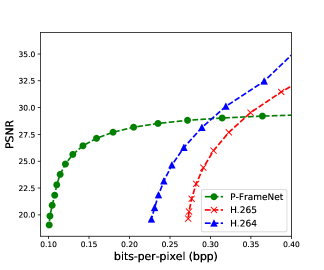
(a) PSNR

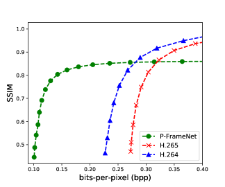
(b) SSIM

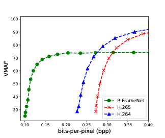
(c) VMAF

Figure 9: P-FrameNet vs. standard video codecs rate-distortion curves.

5.2.2 B-FrameNet vs. Standard Video Codecs

We compare B-FrameNet’s compression efficiency to that of the standard H.264 and H.265 video codecs. Here we compress 18-frame $64\times 64$ videos, each containing two bounding I-frames and sixteen P/B-frames.

Figure 10 compares the PSNR, SSIM and VMAF rate-distortion curves of the various codecs. B-FrameNet outperforms all of the standard video codecs at low-bitrates, which indicates that it is able to produce higher quality inter-frame predictions. This claim is further supported by Figure 11, which shows the difference in quality between H.264, H.265 and B-FrameNet’s inter-frame predictions. We only show the middle five predicted video frames for each codec—those furthest from the I-frames and most reliant on motion compensation. It can be seen that B-FrameNet’s predictions are qualitatively and quantitatively (PSNR, SSIM, VMAF) preferable.

The link below gives a side-by-side example of B-FrameNet’s compression compared to that of H.264 and H.265 at a low bitrate.

https://youtu.be/nV7mLPwOXTI

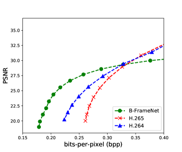
(a) PSNR

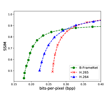
(b) SSIM

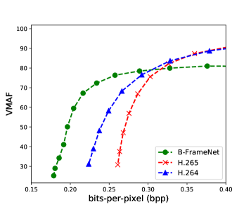
(c) VMAF

Figure 10: B-FrameNet vs. standard video codecs rate-distortion curves.

(a) Ground Truth

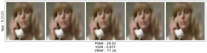
(b) B-FrameNet

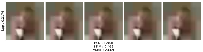
(c) H.264

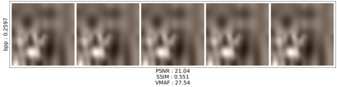
(d) H.265

Figure 11: B-FrameNet vs. standard video codecs inter-frame predictions. We only show the five predicted frames midway between the bounding I-frames.

6 Conclusions

We introduced P-FrameNet and B-FrameNet, deep motion estimation and compensation networks that can replace block-motion algorithms in existing video codecs for improved inter-frame prediction. In contrast to previously developed video codecs, we do not transmit optical flow vectors to guide our video frame predictions. Instead, our encoder network learns to identify and compress the motion present in a video sequence directly. The ensuing binary motion code is used to direct P-FrameNet and B-FrameNet’s decoder in transforming reference frame content. This allows for parallel motion compensation that predicts more complex motion than flow-based methods. Leveraging recent work in deep image compression, we also train P-FrameNet and B-FrameNet to perform 3D dynamic bit assignment, i.e. vary their bit allocations through space-time. We show that this improves compression by focusing bits on complicated video regions. Experiments show that at a lower bitrate, both P-FrameNet and B-FrameNet’s inter-frame predictions are of a higher quality than those of the standard video codecs, H.264 and H.265.

Apart from porting our inter-frame prediction networks into existing deep video codecs, future work will explore replacing flow-based motion estimation in alternative video applications (e.g. slow-motion) with conditioning on our learned binary motion encodings.

References

- Cisco [2017] Cisco, Cisco visual networking index, available at https://www.cisco.com/c/en/us/solutions/collateral/service-provider/visual-networking-index-vni/white-paper-c11-741490.html, 2017.
- Rippel et al. [2018] O. Rippel, S. Nair, C. Lew, S. Branson, A. G. Anderson, L. Bourdev, Learned video compression, arXiv preprint arXiv:1811.06981 (2018).
- Lu et al. [2019] G. Lu, W. Ouyang, D. Xu, X. Zhang, C. Cai, Z. Gao, DVC: an end-to-end deep video compression framework, IEEE Computer Society Conference on Computer Vision and Pattern Recognition (CVPR) (2019).
- Nortje et al. [2019] A. Nortje, W. Brink, H. A. Engelbrecht, H. Kamper, Improved patch-based image compression with BINet: Binary Inpainting Network, In Submission (2019).
- ITU-T H.264 [2003] ITU-T H.264, H.264 advanced video coding for generic audiovisual services, Standard, International Telecommunication Union, 2003.
- ITU-T H.265 [2018] ITU-T H.265, H.265 high efficiency video coding, Standard, International Telecommunication Union, 2018.
- Le Gall [1991] D. Le Gall, MPEG: a video compression standard for multimedia applications, Communications of the Association for Computing Machinery (ACM) (1991).
- Richardson [2010] I. E. G. Richardson, The H.264 advanced video compression standard, 2.0 ed., Wiley, Chichester, West Sussex, 2010.
- Färneback [2003] G. Färneback, Two-frame motion estimation based on polynomial expansion, Scandinavian Conference on Image Analysis (SCIA) (2003).
- VP9 Version 0.6 [2016] VP9 Version 0.6, VP9 bitstream and decoding process specification, Specification, Google, 2016.
- Li et al. [1994] R. Li, B. Zeng, M. L. Lio, A new three-step search algorithm for block motion estimation, IEEE Transactions on Circuits and Systems for Video Technology (TCSVT) (1994).
- Po and Ma [1996] L.-M. Po, W.-C. Ma, A novel four-step search algorithm for fast block motion estimation, IEEE Transactions on Circuits and Systems for Video Technology (TCSVT) (1996).
- Lu and Lio [1997] J. Lu, M. L. Lio, A simple and efficient search algorithm for block-matching motion estimation, IEEE Transactions on Circuits and Systems for Video Technology (TCSVT) (1997).
- Zhu and Ma [2000] S. Zhu, K.-K. Ma, A new diamond search algorithm for fast block-matching motion estimation, IEEE Transactions on Image Processing (TIP) (2000).
- Nie and Ma [2002] Y. Nie, K.-K. Ma, Adaptive rood pattern search for fast block-matching motion estimation, IEEE Transactions on Image Processing (TIP) (2002).
- Haskell et al. [1997] B. G. Haskell, A. Puri, A. N. Netravali, Digital video : an introduction to MPEG-2, Chapman and Hall, 1997.
- De Brabandere et al. [2016] B. De Brabandere, X. Jia, T. Tuytelaars, L. Van Gool, Dynamic filter networks, Conference on Neural Information Processing Systems (NIPS) (2016).
- Liu et al. [2017] Z. Liu, R. A. Yeh, X. Tang, Y. Liu, A. Agarwala, Video frame synthesis using deep voxel flow, International Conference on Computer Vision (ICCV) (2017).
- Niklaus et al. [2017] S. Niklaus, L. Mai, F. Liu, Video frame interpolation via adaptive convolution, IEEE Computer Society Conference on Computer Vision and Pattern Recognition (CVPR) (2017).
- Niklaus and Liu [2018] S. Niklaus, F. Liu, Context-aware synthesis for video frame interpolation, IEEE Computer Society Conference on Computer Vision and Pattern Recognition (CVPR) (2018).
- Jiang et al. [2018] H. Jiang, D. Sun, V. Jampani, M.-H. Yang, E. Learned-Miller, J. Kautz, Super SloMo: high quality estimation of multiple intermediate frames for video interpolation, IEEE Computer Society Conference on Computer Vision and Pattern Recognition (CVPR) (2018).
- Meyer et al. [2018] S. Meyer, A. Djelouah, B. McWilliams, A. Sorkine-Hornung, M. Gross, C. Schroers, PhaseNet for video frame interpolation, IEEE Computer Society Conference on Computer Vision and Pattern Recognition (CVPR) (2018).
- Bao et al. [2019] W. Bao, W.-S. Lai, C. Ma, X. Zhang, Z. Gao, M.-H. Yang, Depth-aware video frame interpolation, IEEE Computer Society Conference on Computer Vision and Pattern Recognition (CVPR) (2019).
- Liu et al. [2019] Y.-L. Liu, Y.-T. Liao, Y.-Y. L. Lin, Y.-Y. Chuang, Deep video frame interpolation using cyclic frame generation, Association for the Advancement of Artificial Intelligence (AAAI) (2019).
- Mathieu et al. [2016] M. Mathieu, C. Couprie, Y. LeCun, Deep multi-scale video prediction beyond mean square error, International Conference on Learning Representations (ICLR) (2016).
- Vondrick et al. [2016] C. Vondrick, H. Pirsiavash, A. Torralba, Generating videos with scene dynamics, Conference on Neural Information Processing Systems (NIPS) (2016).
- Xue et al. [2016] T. Xue, J. Wu, K. L. Bouman, W. T. Freeman, Visual dynamics: probabilistic future frame synthesis via cross convolutional networks, Conference on Neural Information Processing Systems (NIPS) (2016).
- Finn et al. [2016] C. Finn, I. Goodfellow, S. Levine, Unsupervised learning for physical interaction through video prediction, Conference on Neural Information Processing Systems (NIPS) (2016).
- Wu et al. [2018] C.-Y. Wu, N. Singhal, P. Krahenbuhl, Video compression through image interpolation, European Conference on Computer Vision (ECCV) (2018).
- Chen et al. [2018] Z. Chen, T. He, X. Jin, F. Wu, Learning for video compression, IEEE Transactions on Circuits and Systems for Video Technology (TCSVT) (2018).
- Habibian et al. [2019] A. Habibian, T. van Rozendaal, J. M. Tomczak, T. S. Cohen, Video compression with rate-distortion autoencoders, International Conference on Computer Vision (ICCV) (2019).
- Cheng et al. [2019] Z. Cheng, H. Sun, M. Takeuchi, J. Katto, Learning image and video compression through spatial-temporal energy compaction, IEEE Computer Society Conference on Computer Vision and Pattern Recognition (CVPR) (2019).
- Horn and Schunck [1981] B. K. Horn, B. G. Schunck, Determining optical flow, Artificial Intelligence (AI) (1981).
- Ho et al. [2019] Y.-H. Ho, C.-Y. Cho, W.-H. Peng, G.-L. Jin, SME-Net: sparse motion estimation for parametric video prediction through reinforcement learning, International Conference on Computer Vision (ICCV) (2019).
- Johnston et al. [2018] N. Johnston, D. Vincent, D. Minnen, M. Covell, S. Singh, T. Chinen, S. Jin Hwang, J. Shor, G. Toderici, Improved lossy image compression with priming and spatially adaptive bit rates for recurrent networks, IEEE Computer Society Conference on Computer Vision and Pattern Recognition (CVPR) (2018).
- Minnen et al. [2018] D. Minnen, J. Ballé, G. Toderici, Joint autoregressive and hierarchical priors for learned image compression, Conference on Neural Information Processing Systems (NIPS) (2018).
- Li et al. [2018] M. Li, W. Zuo, S. Gu, D. Zhao, D. Zhang, Learning convolutional networks for content-weighted image compression, IEEE Computer Society Conference on Computer Vision and Pattern Recognition (CVPR) (2018).
- Ballé et al. [2018] J. Ballé, D. Minnen, S. Singh, S. J. Hwang, N. Johnston, Variational image compression with a scale hyperprior, arXiv preprint arXiv:1802.01436 (2018).
- Jooyoung Lee and Beack [2019] S. C. Jooyoung Lee, S.-K. Beack, Context-adaptive entropy model for end-to-end optimized image compression, International Conference on Learning Representations (ICLR) (2019).
- Han et al. [2018] J. Han, S. Lombardo, C. Schroers, S. Mandt, Deep probabilistic video compression, arXiv preprint arXiv:1810.02845 (2018).
- Toderici et al. [2015] G. Toderici, S. M. O’Malley, S. J. Hwang, D. Vincent, D. Minnen, S. Baluja, M. Covell, R. Sukthankar, Variable rate image compression with recurrent neural networks, International Conference on Learning Representations (ICLR) (2015).
- Raiko et al. [2014] T. Raiko, M. Berglund, G. Alain, L. Dinh, Techniques for learning binary stochastic feedforward neural networks, arXiv preprint arXiv:1406.2989 (2014).
- Yu and Koltun [2016] F. Yu, V. Koltun, Multi-scale context aggregation by dilated convolutions, International Conference on Learning Representations (ICLR) (2016).
- Baig et al. [2017] M. H. Baig, V. Koltun, L. Torresani, Learning to inpaint for image compression, Conference on Neural Information Processing Systems (NIPS) (2017).
- Rippel and Bourdev [2017] O. Rippel, L. Bourdev, Real-time adaptive image compression, arXiv preprint arXiv:1705.05823 (2017).
- Lowe [2004] D. G. Lowe, Distinctive image features from scale-invariant keypoints, International Journal of Computer Vision (IJCV) (2004).
- Ronneberger et al. [2015] O. Ronneberger, P. Fischer, T. Brox, U-Net: convolutional networks for biomedical image segmentation, International Conference on Medical Image Computing and Computer-Assisted Intervention (MICCAI) (2015).
- Shi et al. [2016] W. Shi, J. Caballero, F. Huszár, J. Totz, A. P. Aitken, R. Bishop, D. Rueckert, Z. Wang, Real-time single image and video super-resolution using an efficient sub-pixel convolutional neural network, IEEE Computer Society Conference on Computer Vision and Pattern Recognition (CVPR) (2016).
- Lathi and Ding [2018] B. P. Lathi, Z. Ding, Modern digital and analog communication systems, 4.0 ed., Oxford University Press, 2018.
- Gautama and Van Hulle [2002] T. Gautama, M. M. Van Hulle, A phase-based approach to the estimation of the optical flow field using spatial filtering, IEEE Transactions on Neural Networks (TNN) (2002).
- Fischer et al. [2015] P. Fischer, A. Dosovitskiy, E. Ilg, P. Häusser, C. Hazırbaş, V. Golkov, P. van der Smagt, D. Cremers, T. Brox, FlowNet: learning optical flow with convolutional networks, International Conference on Computer Vision (ICCV) (2015).
- Ilg et al. [2016] E. Ilg, N. Mayer, T. Saikia, M. Keuper, A. Dosovitskiy, T. Brox, FlowNet 2.0: evolution of optical flow estimation with deep networks, IEEE Computer Society Conference on Computer Vision and Pattern Recognition (CVPR) (2016).
- Zweig and Wolf [2016] S. Zweig, L. Wolf, InterpoNet, A brain inspired neural network for optical flow dense interpolation, IEEE Computer Society Conference on Computer Vision and Pattern Recognition (CVPR) (2016).
- Ranjan and Black [2017] A. Ranjan, M. J. Black, Optical flow estimation using a spatial pyramid network., IEEE Computer Society Conference on Computer Vision and Pattern Recognition (CVPR) (2017).
- Hui et al. [2018] T.-W. Hui, X. Tang, C. C. Loy, LiteFlowNet: a lightweight convolutional neural network for optical flow estimation, IEEE Computer Society Conference on Computer Vision and Pattern Recognition (CVPR) (2018).
- Butler et al. [2012] D. J. Butler, J. Wulff, G. B. Stanley, M. J. Black, A naturalistic open source movie for optical flow evaluation, European Conference on Computer Vision (ECCV) (2012).
- Marszałek et al. [2009] M. Marszałek, I. Laptev, C. Schmid, Actions in context, IEEE Computer Society Conference on Computer Vision and Pattern Recognition (CVPR) (2009).
- NVIDIA [2018a] NVIDIA, NVIDIA open sources NVVL: library for machine learning training, available at https://hub.packtpub.com/nvidia-open-sources-nvvl-library-for-machine-learning-training/, 2018a.
- NVIDIA [2018b] NVIDIA, NVVL, available at https://github.com/NVIDIA/nvvl, 2018b.
- Kingma and Ba [2014] D. P. Kingma, J. Ba, Adam: a method for stochastic optimization, arXiv preprint arXiv:1412.6980 (2014).
- Wang et al. [2004] Z. Wang, A. C. Bovik, H. Rahim Sheikh, E. P. Simoncelli, Image quality assessment: from error visibility to structural similarity, IEEE Transactions On Image Processing (TIP) 13 (2004).
- Netflix [2018a] Netflix, VMAF: the journey continues, available at https://medium.com/netflix-techblog/vmaf-the-journey-continues-44b51ee9ed12, 2018a.
- Netflix [2018b] Netflix, VMAF: video multi-method assessment fusion, available at https://github.com/Netflix/vmaf, 2018b.
- University [2000] A. S. University, Video trace library YUV video sequences, available at http://trace.kom.aau.dk/yuv/index.html, 2000.
- Kamble et al. [2017] S. D. Kamble, N. V. Thakur, P. R. Bajaj, Modified three-step search block matching motion estimation and weighted finite automata based fractal video compression, International Journal of Interactive Multimedia and Artificial Intelligence (IJIMAI) (2017).
- Yang et al. [2010] W. Yang, O. C. Au, C. Pang, J. Dai, F. Zou, An efficient motion vector coding algorithm based on adaptive motion vector prediction, IEEE International Symposium on Circuits and Systems (ISCAS) (2010).