Generalized attenuated ray transforms and their integral angular moments

Abstract

In this article generalized attenuated ray transforms (ART) and integral angular moments are investigated. Starting from the Radon transform, the attenuated ray transform and the longitudinal ray transform, we derive the concept of ART-operators of order $k$ over functions defined on the phase space and depending on time. The ART-operators are generalized for complex-valued absorption coefficient as well as weight functions of polynomial and exponential type. Connections between ART operators of various orders are established by means of the application of the linear part of a transport equation. These connections lead to inhomogeneous differential equations of order $(k+1)$ for the ART of order $k$. Uniqueness theorems for the corresponding boundary-value and initial boundary-value problems are proved. Properties of integral angular moments of order $p$ are considered and connections between the moments of different orders are deduced. A close connection of the considered operators with mathematical models for tomography, physical optics and integral geometry allows to treat the inversion of ART of order $k$ as an inverse problem of determining the right-hand side of a corresponding differential equation.

1 Introduction and preliminaries

Many linear integral operators arising as mathematical models in computer and emission tomography, wave optics, integral geometry of tensor fields, can be classified as generalized attenuated ray transforms (ART) that act on functions or tensor fields.

In recent years a significant progress of emission tomography in biology and medicine diagnostics can be observed, see [5, 23]. In contrast to transmission computer tomography, the mathematical setting of emission tomography problem contains, in general, two unknown functions that have to be reconstructed. The first function (absorption coefficient) characterizes the absorption within the medium whereas the second describes the distribution of internal sources whose radiation is measured by detectors. The goal is to find the distribution of internal sources $f$ and/or the absorption coefficient $\varepsilon$ by given values of the attenuated ray transform

(1) $$I=\int\limits_{L}f(q)\exp\left(-\int_{L(q)}\varepsilon(p)\,dp\right)dq,$$

where $L(q)$ is the segment of the straight line $L$ between a source point $q$ and the detector. In most mathematical settings of emission tomography the absorption coefficient is supposed to be known. Absorption phenomena also arise in models of vector tomography [15, 2, 20]. The authors there investigate important theoretical questions and use these as starting point to handle some aspects of vector tomography.

Another reason for investigating generalized ARTs are motivated by the research area of physical optics, more specifically wave optics and photometry.

We specifiy the mathematical models. Let a rectangular Cartesian coordinate system be given in the Euclidean space ${\mathbb{R}}^{3}$ with inner product $\langle x,y\rangle$ and norm $|x|$ of elements $x=(x^{1},x^{2},x^{3})$, $y=(y^{1},y^{2},y^{3})\in{\mathbb{R}}^{3}$. We denote the unit sphere by $\SS^{2}$, and $\SS{\mathbb{R}}:={\mathbb{R}}^{3}\times\SS^{2}=\{(x,\xi)\,|\,x\in{\mathbb{R}}^{3},\xi\in\SS^{2}\}$. For a bounded convex domain $D\subset{\mathbb{R}}^{3}$ with smooth boundary $\partial D$ we define $\SS D:=\{(x,\xi)\,|\,x\in D,\xi\in\SS^{2}\}$. The sets $\SS{\mathbb{R}}$ and $\SS D$ are known as the spherical bundles for ${\mathbb{R}}^{3}$ and $D$. The set of pairs $(x,\xi)\in\SS{\mathbb{R}}$ with fixed $x$ is denoted as $\SS^{2}_{x}$. We assume that the domain $D$ contains a distribution $f(q)$, $q\in D$, of sources of a monochromatic wave field. Using the notation of the optical system [17], which represents a mathematical formalization of a device like a camera, see Fig. 1, leads to the formulation of the direct problem of wave optics consisting in solving a boundary-value problem for the Helmholtz equation satisfying discontinuous boundary conditions of Kirchhoff type, see [4],

(2) $$\left\{\begin{array}[]{rr}\Delta u+k^{2}u&=0\\ u|_{\Sigma}&=u_{n}\\ u|_{L\backslash\Sigma}&=0,\end{array}\right.$$

as well as the Sommerfeld radiation condition,

(3) $$\frac{\partial u}{\partial|x|}-{\rm i}ku=o\left(\frac{1}{|x|}\right)\quad\mbox{at}\,\,|x|\rightarrow\infty.$$

Here $u_{n}$ is a wave field hitting a diaphragm $\Sigma$, ${\rm i}$ is the imaginary unit and $k$ is the wave number.

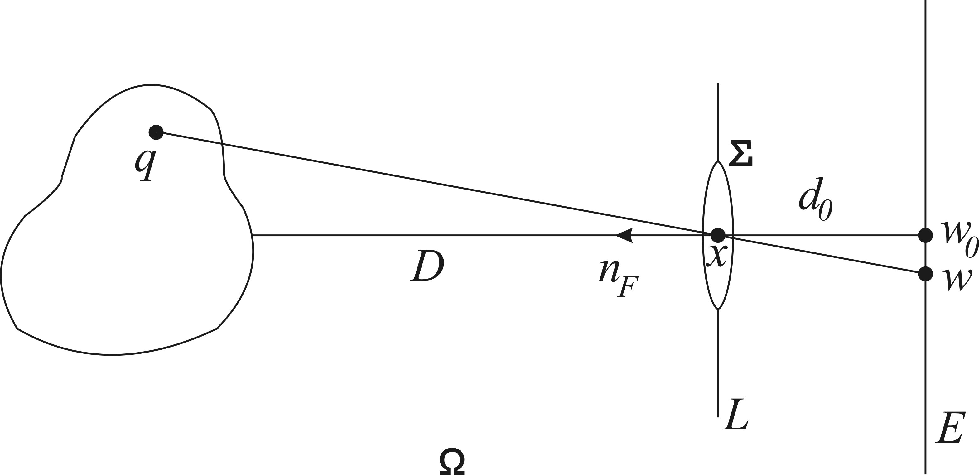
Figure 1: Scheme of optical system.

The optical system $\Omega$ depicted in Fig. 1 consists of the plane $L$, in which the diaphragm $\Sigma$ with center $x$ is located, $n_{F}$ denotes the outer unit normal vector to $\Sigma$, $E$ is a screen with center $w_{0}$, $d_{0}$ is the focal distance between $L$ and $E$ and $w$ the geometrical image of a point $q\in D$. An application of Green’s function for the half-space yields a solution $u$ of the direct problem for (2) represented as a Kirchhoff integral [4]. Usually in optics the Fraunhofer approximation for the far field is used [13] which allows to simplify the solution significantly. The obtained approximate solution $u$ for (2) is then represented as a convolution $u=\widetilde{u}_{\delta}\ast\Delta$ with known kernel $\Delta$. Function $\widetilde{u}_{\delta}$ is called the ideal wave image [16] and has the representation

(4) $$\widetilde{u}_{\delta}(x,\xi)=\int\limits_{0}^{\infty}s{e^{iks}}f(x-s\xi)ds.$$

A similar setting of the direct problem with incoherent sources in $D$ and given constant absorption coefficient $\varepsilon>0$ leads to so called ideal photometric image

(5) $$\widetilde{u}_{\delta}(x,\xi)=\int\limits_{0}^{\infty}{e^{-\varepsilon s}}f(x-s\xi)ds.$$

The inverse problems of wave optics and photometry are formulated as reconstruction problems for a function $f$ which describes distributions of sources of a monochromatic wave field or distributions of incoherent sources. The initial data for these inverse problems are integrals along all straight lines of ${\mathbb{R}}^{3}$ in the right-hand parts of (4), (5). In other words we use the integrals with lower limit $-\infty$ as initial data for the corresponding inverse problems.

Tensor tomography traditionally has applications to the problems of photoelasticity and fiber optics [1]. New approaches and achievements emerge in diffractive tomography of strains [18], diffusion MRI-tomography and cross-polarization optic coherent tomography [24, 12]. Success of tensor tomography in studying of anisotropic objects and materials in physics, geophysics, biology and medicine has deep impact and is closely connected with the progress in integral geometry of tensor fields, wherein many types of ray transforms are investigated [27], see furthermore [10, 28, 11, 7] for the 2D-case and [19, 21] for arbitrary dimensions of Euclidean space or Riemannian manifolds.

As initial data for inverse problems in integral geometry connected to tensor fields are in particular reprsented by the longitudinal ray transform

(6) $${\cal P}w(x,\xi)=\int\limits^{\infty}_{0}w_{i_{1}\ldots i_{m}}(x-s\xi)\xi^{i_{1}}\ldots\xi^{i_{m}}ds,$$

where $w_{i_{1}\ldots i_{m}}(x)$ is a symmetric tensor field of rank $m$ ($m$-tensor field), $\xi^{l}$ are the components of the vector of direction $\xi$, $|\xi|=1$, of a straight line $L$ along which the integration is computed. Here and subsequently Einstein’s summation rule is used, which says that by repeating super- and subscripts in a monomial a summation from $1$ to $n$ is meant ($n$ is the dimension of the Euclidean space). The aim is to recover a tensor field $w$ from given values of its longitudinal ray transform (6).

In this article the operators of ART for functions and tensor fields are generalized in four different respects. At first, the functions $f(x)$ and $\varepsilon(x)$ depend not only on the spatial variable $x$, but also on the unit vector of direction $\xi$. Secondly, the absorption coefficient $\varepsilon$ is a complex-valued function similar to those arising in inverse scattering problems when Rytov’s approach is applied  [22, 3], and then in the framework of diffraction tomography, see, e.g.,[23]. Next we take into account the concept of polynomially weighted ray transform of tensor fields as represented in [27]. The final generalization is connected with settings of dynamic tomography [25, 26, 14] and consists in consideration the situation that the internal sources depend on time $t$. In other words we suppose the function $f(t,x,\xi)$ to depend on time $t$, space $x$ and vector of direction $\xi$. We use the notation $\alpha(x,\xi)$ for a complex-valued function $\varepsilon(x,\xi)+{\rm i}\rho(x,\xi)$.

The attenuated ray transform (ART) of order $k$ is defined by

(7) $$u_{k}(x,\xi)\displaystyle{=\int\limits^{\infty}_{0}s^{k}\exp\left(-\int^{s}_{0}\alpha(x-\sigma\xi,\xi)d\sigma\right)f(x-s\xi,\xi)ds.}$$

Functions $\varepsilon\geq 0$, $\rho$ and $f$ are finite and bounded with respect to the variable $x$. In particular, the function $f(x,\xi)$ may have a form as

(8) $$f(x,\xi)=w_{i_{1}\ldots i_{m}}(x)\xi^{i_{1}}\ldots\xi^{i_{m}}.$$

coinciding with the integrand in (6).

Formula (7) defines a stationary ART of order $k$. Suppose that $f$ is a function depending on time $t$, too, and the propagation speed of perturbation be, for simplicity, equal to unity. Then,

(9) $$u_{k}(t,x,\xi)\displaystyle{=\int\limits^{\infty}_{0}s^{k}\exp\left(-\int^{s}_{0}\alpha(x-\sigma\xi,\xi)d\sigma\right)f(t-s,x-s\xi,\xi)ds,}$$

is called the non-stationary ART of order $k$. In particular, the function $f(t,x,\xi)$ may be defined as

$$f(t,x,\xi)=w_{i_{1}\ldots i_{m}}(t,x)\xi^{i_{1}}\ldots\xi^{i_{m}}.$$

Inversion formulas for the Radon transform ${\mathcal{R}}\varphi$ of a function $\varphi(x)$, such as

(10) $${\mathcal{R}}\varphi(\eta,s)=\int\limits_{R^{3}}\varphi(x)\delta(\langle\eta,x\rangle-s)dx,$$

where $\delta(\cdot)$ denotes the $\delta$-function on $R$ and $\eta$ is the unit normal vector to the plane of integration, do often involve the back-projection operator ${\mathcal{R}}^{\#}$, acting on the Radon transform,

(11) $${\mathcal{R}}^{\#}g(x)=\frac{1}{4\pi^{2}}\int\limits_{\SS^{2}_{x}}g(\eta,\langle\eta,x\rangle)d\lambda_{x}(\xi),$$

where $g(\eta,s)$ $=$ ${\mathcal{R}}\varphi(\eta,s)$ and $d\lambda_{x}(\xi)$ is the angular measure on the sphere $\SS^{2}_{x}$.

The back-projection operator acting on the longitudinal ray transform (6) is represented by

(12) $${\mathcal{P}}^{\#}h(x)=\frac{1}{4\pi^{2}}\int\limits_{\SS^{2}_{x}}\xi^{i_{1}}\ldots\xi^{i_{m}}h(x,\xi)\,d\lambda_{x}(\xi),$$

where $h(x,\xi)$ $=$ ${\mathcal{P}}w(x,\xi)$ (see formula (6)). The image of the back-projection operator (12) is a symmetric tensor field $\mu_{m}^{i_{1}\ldots i_{m}}$ of rank $m$, $\mu_{m}:={\mathcal{P}}^{\#}{\mathcal{P}}w(x)$.

In the articles [11, 7, 8, 9] integral angular moments in 2D have been introduced as generalizations of back-projection operators. The suggested operators, acting on arbitrary tomographic transforms, are of utmost importance for recovering the singular support of a tensor field by its known ART similar to (7). The mathematical model is convenient for a medium with refraction and variable absorption coefficient which may be unknown. In this article the integral angular moments are defined in a more general way then in 2D only. They map a generalized ART of order $k$, $u_{k}$, with respect to functions $f(x,\xi)$ or $f(t,x,\xi)$ to 3D-symmetric tensor fields.

As mentioned before the definition of the integral angular moment ${\cal E}_{kp}^{i_{1}\dots i_{p}}(u)$ of ART $u_{k}$ of order $k$ can be seen as a generalization of the back-projection operator. It is defined by

(13) $${\cal E}_{kp}^{i_{1}\dots i_{p}}u(x)=\int\limits_{\SS^{2}_{x}}u_{k}(x,\xi)\xi^{i_{1}}\dots\xi^{i_{p}}\,d\lambda_{x}(\xi),\quad p\geq 0.$$

In particular, if $f(x,\xi)$ is given as in (8), then the integral angular moment (13) coincides with the back-projection operator of the longitudinal ray transform.

Outline. The first section of the article deals with certain connections between generalized ART of different orders. We deduce differential equations of order $k+1$, whose solutions are the ART of order $k$ acting on a function $f(x,\xi)$ or, in the general case, on a $m$-tensor field $w(x)$. Differential equations of the first order coincide with stationary and non-stationary transport equations with right-hand side $f(x,\xi)$, complex-valued absorption coefficient $\alpha(x,\xi)$, and without the integral part that describes the scattering [6]. The second section is devoted to proofs of uniqueness theorems for the emerging boundary-value and initial boundary-value problems of arbitrary order. The third section contains properties of the integral angular moments over ART of order $k$. Connections of certain differential operators and the operators of divergence with the operators of integral angular moments are established. We conclude the article by emphasizing the connections between generalized ART and different mathematical models of tomography, physical optics and integral geometry and an outlook to future research in the field.

2 Main equations

We start by defining differential equations whose solutions are attenuated ray transforms (ART) of order $k$ of functions $f(x,\xi)$.

The operator ${\mathcal{H}}$, acting on functions $\psi(x,\xi)$ that are differentiable on $\SS{\mathbb{R}}$, is defined in invariant form by

(14) $${\mathcal{H}}\psi(x,\xi)=\frac{d}{d\tau}\psi(x+\tau\xi,\xi)\Big{|}_{\tau=0}.$$

In a rectangular Cartesian coordinate system the operator is represented as

(15) $${\mathcal{H}}\psi(x,\xi)=\xi^{1}\frac{\partial\psi}{\partial x^{1}}+\xi^{2}\frac{\partial\psi}{\partial x^{2}}+\xi^{3}\frac{\partial\psi}{\partial x^{3}}=\langle\xi\,,\nabla\psi\rangle={\rm div}\,(\psi\xi).$$

Lemma 1.

Let $\varepsilon(x,\xi)\geq 0$, $\rho(x,\xi)$, $f(x,\xi)$ be elements of $C^{1}(\SS D)$. Then for $u_{k}(x,\xi)$ defined by (7), $k\geq 1$ being an integer, the identity

(16) $$\big{(}({\mathcal{H}}+\alpha)u_{k}\big{)}(x,\xi)=k\,u_{k-1}(x,\xi)$$

is valid.

Proof.

We prove relation (16) directly. By definition (14),

$$\begin{array}[]{rcl}{\mathcal{H}}u_{k}(x,\xi)&=&{\displaystyle\frac{d}{d\tau}u_{k}(x+\tau\xi,\xi)\Big{|}_{\tau=0}}\\[12.91663pt] &=&{\displaystyle\int\limits^{\infty}_{0}s^{k}\left.\frac{d}{d\tau}\exp\left(-\int^{s}_{0}\alpha(x+(\tau-\sigma)\xi,\xi)d\sigma\right)\right|_{\tau=0}f(x-s\xi,\xi)ds}\\[17.22217pt] &&{\displaystyle+\int\limits^{\infty}_{0}s^{k}\exp\left(-\int^{s}_{0}\alpha(x-\sigma\xi,\xi)d\sigma\right)\frac{d}{d\tau}f\big{(}x+(\tau-s)\xi,\xi\big{)}\Big{|}_{\tau=0}ds}.\end{array}$$

For fixed $x$ and vector $\xi$ the functions $f(x+v\xi,\xi)$ and $\alpha(x+v\xi,\xi)$ can be treated as functions depending only on a real variable $v$,

$$f(x+v\xi)=\varphi(v),\quad\alpha(x+v\xi,\xi)=\psi(v).$$

Then,

$$\frac{d}{d\tau}\varphi(\tau-s)=-\frac{d}{ds}\varphi(\tau-s),\quad\frac{d}{d\tau}\psi(\tau-\sigma)=-\frac{d}{d\sigma}\psi(\tau-\sigma),$$

and hence

$$\begin{array}[]{rcl}{\mathcal{H}}u_{k}(x,\xi)&=&\displaystyle{\int\limits^{\infty}_{0}s^{k}\varphi(-s)\exp\left(-\int^{s}_{0}\psi(-\sigma)d\sigma\right)\int^{s}_{0}\frac{d}{d\sigma}\psi(\tau-\sigma)\Big{|}_{\tau=0}d\sigma\,ds}\\[17.22217pt] &&\displaystyle{-\int\limits^{\infty}_{0}s^{k}\exp\left(-\int^{s}_{0}\psi(-\sigma)d\sigma\right)\left.\frac{d\varphi(\tau-s)}{ds}\right|_{\tau=0}ds}.\end{array}$$

Passing to the limit $\tau\rightarrow 0$ and applying integrating by parts in the second term of the right-hand part yield

(17) $$\begin{array}[]{rcl}{\mathcal{H}}u_{k}(x,\xi)&=&\displaystyle{\int\limits^{\infty}_{0}s^{k}\exp\left(-\int^{s}_{0}\psi(-\sigma)d\sigma\right)\varphi(-s)\big{[}\psi(-s)-\psi(0)\big{]}ds}\\[17.22217pt] &&\displaystyle{}-s^{k}\exp\left(-\int^{s}_{0}\psi(-\sigma)d\sigma\right)\varphi(-s)\Big{|}^{\infty}_{s=0}\\[17.22217pt] &&{}+\displaystyle{\,k\int\limits^{\infty}_{0}s^{k-1}\exp\left(-\int^{s}_{0}\psi(-\sigma)d\sigma\right)\varphi(-s)ds\vspace*{1mm}}\\[17.22217pt] &&{}-\displaystyle{\int\limits^{\infty}_{0}s^{k}\exp\left(-\int^{s}_{0}\psi(-\sigma)d\sigma\right)\varphi(-s)\left[\frac{d}{ds}\int^{s}_{0}\psi(-\sigma)d\sigma\right]ds}.\end{array}$$

Since the function $f(x,\xi)$ is finite with respect to $x$, $s^{k}=0$ at $k\geq 1$ and $s=0$, the second term vanishes for $s\rightarrow\infty$ and $s=0$. The third term on the right-hand side is equal to $ku_{k-1}(x,\xi)$ according to (7). Summing up the first and the last items we obtain $-\alpha(x,\xi)u_{k}(x,\xi)$. Thus,

$${\mathcal{H}}u_{k}(x,\xi)=ku_{k-1}(x,\xi)-\alpha(x,\xi)u_{k}(x,\xi),$$

and the equality (16) is proved. ∎

Lemma 2.

Let $\varepsilon(x,\xi)\geq 0$, $\rho(x,\xi)$, $f(x,\xi)$ be elements of $C^{1}(SD)$. Then the function $u_{0}(x,\xi)$ defined by (7) is a solution of the equation

(18) $$({\mathcal{H}}+\alpha)u_{0}(x,\xi)=f(x,\xi).$$

Proof.

Arguments that are similar to those of the proof of lemma 1 lead to following equality,

(19) $$\begin{array}[]{rcl}{\mathcal{H}}u_{0}(x,\xi)&=&\displaystyle{\int\limits^{\infty}_{0}\varphi(-s)\exp\left(-\int^{s}_{0}\psi(-\sigma)d\sigma\right)\psi(-s)ds}\\[17.22217pt] &&{}-\displaystyle{\int\limits^{\infty}_{0}\varphi(-s)\exp\left(-\int^{s}_{0}\psi(-\sigma)d\sigma\right)\psi(0)ds}\\[17.22217pt] &&{}-\displaystyle{\,\exp\left(-\int^{s}_{0}\psi(-\sigma)d\sigma\right)\varphi(-s)\Big{|}^{\infty}_{s=0}}\\[17.22217pt] &&{}-\displaystyle{\int\limits^{\infty}_{0}\varphi(-s)\exp\left(-\int^{s}_{0}\psi(-\sigma)d\sigma\right)\left[\frac{d}{ds}\int^{s}_{0}\psi(-\sigma)d\sigma\right]ds}\end{array}$$

instead of (17). It is easy to see that the first and the last terms on the right-hand side differ only by signs and so their sum is equal to zero. The second term is equal to $-\psi(0)\,u_{0}(x,\xi)$, and the third is equal to $\varphi(0)$. As $\varphi(0)=f(x,\xi)$, $\psi(0)=\alpha(x,\xi)$ we have ${\mathcal{H}}u_{0}(x,\xi)=f(x,\xi)-\alpha(x,\xi)u_{0}(x,\xi)$ and the statement of lemma 2 is verified. ∎

We consider the important partial case if the function $f(x,\xi)$ in (7) has a form (8) which is a $m$-homogeneous polynomial in $\xi^{j}$. The set of all given symmetric $m$-tensor fields $w(x)=(w_{i_{1}\ldots i_{m}}(x))$, $i_{1},\ldots,i_{m}=1,2,3$, in ${\mathbb{R}}^{3}$ or in $D$ is denoted by $S^{m}(D)$. For simplicity we usually write $S^{m}$. The scalar product in $S^{m}$ is defined by

(20) $$\langle u(x),v(x)\rangle=u_{i_{1}\ldots i_{m}}(x)v^{i_{1}\ldots i_{m}}(x),$$

and we use the notation $\langle w,\xi^{m}\rangle$ for the sum $w_{i_{1}\ldots i_{m}}\xi^{i_{1}}\ldots\xi^{i_{m}}$. In Euclidean space with rectangular Cartesian coordinate system there is no difference between contravariant and covariant components of tensors. In this article we usually use covariant components of tensors.

Corollary 3.

Let $\varepsilon(x,\xi)\geq 0$, $\rho(x,\xi)$, $f(x,\xi)$ be elements of $C^{1}(\SS D)$. Let the function $f(x,\xi)$ in (7) be of a form $\langle w(x),\xi^{m}\rangle$ (8), where $w(x)$, $x\in D$, is a symmetric $m$-tensor field, $m\geq 0$ being an integer. Then $u_{0}(x,\xi)$ is a solution of the equation

(21) $$\big{(}({\mathcal{H}}+\alpha)u_{0}\big{)}(x,\xi)=\langle w,\xi^{m}\rangle.$$

Proof.

Since lemma 2 is valid for any function $f(x,\xi)$, it also holds for each component $w_{i_{1}\ldots i_{m}}(x)$ of symmetric $m$-tensor field $w(x)$. We take into account now the linearity of the inner product and get

(22) $$\begin{array}[]{c}\displaystyle{\int\limits^{\infty}_{0}s^{k}\exp\left(-\int^{s}_{0}\alpha(x-\sigma\xi,\xi)d\sigma\right)\langle w(x-s\xi)\,,\,\xi^{m}\rangle ds}\\[17.22217pt] \quad=\displaystyle{\left\langle\xi^{m}\,,\,\int\limits^{\infty}_{0}s^{k}\exp\left(-\int^{s}_{0}\alpha(x-\sigma\xi,\xi)d\sigma\right)w(x-s\xi)ds\right\rangle}.\end{array}$$

This gives (21). ∎

We define an operator ${\mathcal{L}}_{k}$ $:$ $C^{k}(\SS{\mathbb{R}})$ $\rightarrow$ $C(\SS{\mathbb{R}})$ by

$${\mathcal{L}}_{1}\psi(x,\xi)=({\mathcal{H}}+\alpha)\psi(x,\xi),$$

$$\hskip 28.45274pt{\mathcal{L}}_{k}\psi(x,\xi)=\frac{1}{k-1}({\mathcal{H}}+\alpha){\mathcal{L}}_{k-1}\psi(x,\xi),$$

for $k>1$ being an integer.

Theorem 4.

Let $\varepsilon(x,\xi)\geq 0$, $\rho(x,\xi)$, $f(x,\xi)$ be elements of $C^{k+1}(\SS D)$, $w(x)\in C^{k+1}(S^{m})$, $x\in D$, be a symmetric $m$-tensor field. Then for an integer $k\geq 0$, the function $u_{k}(x,\xi)$ is a solution of the equation

(23) $${\mathcal{L}}_{k+1}u_{k}(x,\xi)=f(x,\xi)$$

In particular for $f(x,\xi)=\langle w(x),\xi^{m}\rangle$, the equality for $m\geq 0$

(24) $${\mathcal{L}}_{k+1}u_{k}(x,\xi)=\big{\langle}w(x),\xi^{m}\big{\rangle}$$

is valid with $u_{k}(x,\xi)$ defined by (7).

Proof.

Under the assumptions of lemma 1, we apply on the both sides of (16) $(k-1)$ times the operator $({\mathcal{H}}+\alpha)$. This gives $({\mathcal{H}}+\alpha)^{k}u_{k}(x,\xi)=u_{0}(x,\xi)$. Applying the operator $({\mathcal{H}}+\alpha)$ once more and using lemma 2, we get the first statement (23) of the theorem. Applying these arguments to $f(x,\xi)=\langle w(x),\xi^{m}\rangle$ we get formula (24). ∎

Thus we have differential relations (23), (24), connecting ART $u_{k}(x,\xi)$ of order $k$ with the function $f(x,\xi)$ or symmetric $m$-tensor field $w(x)$.

We advance to the non-stationary case.

Lemma 5.

For functions $\varepsilon(x,\xi)\geq 0$, $\rho(x,\xi)$ $\in$ $C^{1}(\SS D)$, $f(t,x,\xi)$ $\in$ $C^{1}(R\times\SS D)$. Then for $u_{k}(t,x,\xi)$ determined by (9), $k\geq 0$, the equalities

(25) $$\hskip 11.38109pt\Big{(}\frac{\partial}{\partial t}+{\mathcal{H}}+\alpha\Big{)}u_{k}=k\,u_{k-1},\quad k\geq 1\,,$$

(26) $$\Big{(}\frac{\partial}{\partial t}+{\mathcal{H}}+\alpha\Big{)}u_{0}=f$$

are valid. In particular, if $f(t,x,\xi)=\langle w(t,x),\xi^{m}\rangle$ for a symmetric $m$-tensor field $w(t,x)\in C^{1}({\mathbb{R}}\times S^{m})$, then the equality

(27) $$\Big{(}\frac{\partial}{\partial t}+{\mathcal{H}}+\alpha\Big{)}u_{0}=\big{\langle}w,\xi^{m}\big{\rangle}$$

holds true.

Proof.

Fixing non-stationary ART $u_{k}(t,x,\xi)$ of order $k$ defined by (9), we find $\displaystyle{\frac{\partial u_{k}}{\partial t}(t,x,\xi)}$. Since only function $f$ depends on $t$, we have to compute $\displaystyle{\frac{\partial f(t-s,x-s\xi,\xi)}{\partial t}}$,

(28) $$\frac{\partial u_{k}}{\partial t}=\int\limits^{\infty}_{0}s^{k}\exp\left(-\int^{s}_{0}\alpha(x-\sigma\xi,\xi)d\sigma\right)\frac{\partial f(t-s,x-s\xi,\xi)}{\partial t}ds.$$

We calculate the total derivative $\displaystyle{\frac{df}{ds}}$ at first,

$$\frac{df}{ds}=\left\langle\frac{\partial f(t-s,x-s\xi,\xi)}{\partial(x-s\xi)},\;\frac{\partial(x-s\xi)}{\partial s}\right\rangle+\frac{\partial f(t-s,x-s\xi,\xi)}{\partial(t-s)}\,\frac{\partial(t-s)}{\partial s}.$$

Using

$$\,\displaystyle{\frac{\partial f(\theta,y,\xi)}{\partial y}}=\nabla_{y}f(\theta,y,\xi)$$

for $y=x-s\xi$, $\theta=t-s$, and $\,\displaystyle{\frac{\partial y}{\partial s}=-\xi}$, the derivative is represented as

$$\frac{df}{ds}=\left\langle\nabla_{y}f(\theta,y,\xi)\,,-\xi\right\rangle+\frac{\partial f(\theta,y,\xi)}{\partial\theta}\,\frac{\partial\theta}{\partial s}.$$

The next step consists in calculation the result of ${\mathcal{H}}$ action on $f$,

$${\mathcal{H}}f\equiv\displaystyle{\frac{df(\theta,y+\tau\xi,\xi)}{d\tau}\Big{|}_{\tau=0}}=\displaystyle{\left\langle\frac{\partial f(\theta,y+\tau\xi,\xi)}{\partial(y+\tau\xi)}\,,\,\frac{\partial(y+\tau\xi)}{\partial\tau}\right\rangle\Big{|}_{\tau=0}}=\displaystyle{\left\langle\nabla_{y}f(\theta,y,\xi)\,,\xi\right\rangle}.$$

Because of $\displaystyle{\frac{\partial\theta}{\partial s}}$ $=$ $\displaystyle{-\frac{\partial\theta}{\partial t}}$ we obtain

$${\frac{\partial f(\theta,y,\xi)}{\partial t}}=\displaystyle{-\frac{df(\theta,y+\tau\xi,\xi)}{d\tau}\Big{|}_{\tau=0}-\frac{df(\theta,y,\xi)}{ds}.}$$

This implies

$$\begin{array}[]{rcl}\displaystyle{\frac{\partial u_{k}}{\partial t}(t,x,\xi)}&=&\displaystyle{-\int\limits^{\infty}_{0}s^{k}\exp\left(-\int^{s}_{0}\alpha(x-\sigma\xi,\xi)d\sigma\right)\frac{df(t-s,x+(\tau-s)\xi,\xi)}{d\tau}\Big{|}_{\tau=0}ds\vspace*{2mm}}\\[17.22217pt] &&{}-\displaystyle{\int\limits^{\infty}_{0}s^{k}\exp\left(-\int^{s}_{0}\alpha(x-\sigma\xi,\xi)d\sigma\right)\frac{df(t-s,x-s\xi,\xi)}{ds}\,ds.}\end{array}$$

Based on the definition of operator ${\mathcal{H}}$ we integrate the second term of the right-hand side of the last expression and obtain

$$\begin{array}[]{rcl}\displaystyle{\Big{(}\frac{\partial u_{k}}{\partial t}}\displaystyle{+{\mathcal{H}}u_{k}\Big{)}(t,x,\xi)}&=&\displaystyle{\int\limits^{\infty}_{0}s^{k}\left.\frac{d}{d\tau}\exp\left(-\int^{s}_{0}\alpha(x+(\tau-\sigma)\xi,\xi)d\sigma\right)\right|_{\tau=0}}\,f(t-s,x-s\xi,\xi)ds\\[17.22217pt] &&{}-\displaystyle{\,s^{k}\exp\left(-\int^{s}_{0}\alpha(x-\sigma\xi,\xi)d\sigma\right)f(t-s,x-s\xi,\xi)\Big{|}^{\infty}_{s=0}}\\[17.22217pt] &&{}+\displaystyle{\int\limits^{\infty}_{0}f(t-s,x-s\xi,\xi)\frac{d}{ds}\left[s^{k}\exp\left(-\int^{s}_{0}\alpha(x-\sigma\xi,\xi)d\sigma\right)\right]ds.}\end{array}$$

We refer to the reasonings and calculations similar to those in the proofs of lemmas 1 and 2. As before, taking into account the different results depending on $k\geq 1$ or $k=0$, we obtain (25), (26) of lemma 5 for non-stationary ART $u_{k}$ over the function $f(t,x,\xi)$. In partial case $f(t,x,\xi)=\langle w(t,x),\xi^{m}\rangle$, where $w(t,x)$ is a symmetric $m$-tensor field, the equality (27) is verified instead of (26). As it was before the linearity property (22) has been applied. ∎

We define the operator ${{\mathcal{L}}}^{t}_{k}:C^{k}(R\times\SS D)\rightarrow C(R\times\SS D)$ by mathematical induction on $m$,

$$\begin{array}[]{rcl}\displaystyle{{{\mathcal{L}}}^{t}_{1}\psi(t,x,\xi)}&=&\displaystyle{\Big{(}\frac{\partial}{\partial t}+{\mathcal{H}}+\alpha\Big{)}\psi(t,x,\xi)},\vspace*{3mm}\\ {{\mathcal{L}}}^{t}_{k}\psi(t,x,\xi)&=&\displaystyle{\Big{(}\frac{\partial}{\partial t}+{\mathcal{H}}+\alpha\Big{)}{{\mathcal{L}}}^{t}_{k-1}\psi(t,x,\xi)},\quad k>1.\end{array}$$

Theorem 6.

For $\varepsilon(x,\xi)\geq 0$, $\varepsilon(x,\xi),\rho(x,\xi)$ $\in$ $C^{k+1}(\SS D)$, $f(t,x,\xi)\in C^{k+1}(R\times\SS D)$, the function $u_{k}(t,x,\xi$ defined by (9) is a solution of the equation

(29) $$({{\mathcal{L}}}^{t}_{k+1}u_{k})(t,x,\xi)=f(t,x,\xi).$$

In particular, the function defined by (9) $u_{k}(t,x,\xi$ containing $f(t,x,\xi)=\langle w(t,x),\xi^{m}\rangle$, where $w$ is symmetric $m$-tensor field, is a solution of the equation

(30) $$({{\mathcal{L}}}^{t}_{k+1}u_{k})(t,x,\xi)=\big{\langle}w(t,x),\xi^{m}\big{\rangle}.$$

Proof.

The proof is based on lemma 5 and follows the lines of the proof of theorem 4. ∎

3 Uniqueness theorems

We prove uniqueness theorems for boundary-value and initial boundary-value problems of the equations (23), (29), respectively. We remind that $D\subset{\mathbb{R}}^{3}$ is a bounded convex domain with smooth boundary $\partial D$.

Theorem 7.

Let for $\varepsilon(x,\xi),\rho(x,\xi)\in C^{k}(\SS D)$, $\varepsilon(x,\xi)\geq 0$, a function $\varphi(x,\xi)\in C^{k+1}(\SS D)$ be a solution of the equation

(31) $$\frac{1}{k!}\big{(}{\mathcal{H}}+\alpha\big{)}^{k+1}\varphi=0$$

and satisfies the boundary-value conditions

(32) $$\varphi(x,\xi)=({\mathcal{H}}\varphi)(x,\xi)=\dots=({\mathcal{H}}^{k}\varphi)(x,\xi)=0,\quad x\in\partial D,\quad\langle n_{x},\xi\rangle<0,$$

where $n_{x}$ is the outer normal to the surface $\partial D$ at a point $x$. Then $\varphi(x,\xi)\equiv 0$ for $(x,\xi)\in\SS D$.

Proof.

We prove the statement for $k=0$ at first. For this case (31) reads as $({\mathcal{H}}+\alpha)\varphi=0$. Since the coefficient $\alpha(x,\xi)=\varepsilon(x,\xi)+{\rm i}\rho(x,\xi)$ in (32) is complex-valued, the function $\varphi(x,\xi)$ is complex-valued too, and thus it can be represented in a form $\varphi=\varphi_{1}+{\rm i}\varphi_{2}$. We write $({\mathcal{H}}+\alpha)\varphi$ in more details,

$$({\mathcal{H}}+\varepsilon+{\rm i}\rho)(\varphi_{1}+{\rm i}\varphi_{2})=({\mathcal{H}}\varphi_{1}+\varepsilon\varphi_{1}-\rho\varphi_{2})+{\rm i}({\mathcal{H}}\varphi_{2}+\varepsilon\varphi_{2}+\rho\varphi_{1})=0,$$

and multiply the obtained formula with $\bar{\varphi}=\varphi_{1}-{\rm i}\varphi_{2}$. Here, the notations $\bar{\varphi}$ for complex conjugate and $|\varphi|$ for modulus of complex-valued function $\varphi$ are used. Then,

$$Re\left\{\bar{\varphi}({\mathcal{H}}+\bar{\alpha})\varphi\right\}=\frac{1}{2}{\mathcal{H}}(|\varphi|^{2})+\varepsilon|\varphi|^{2}=0.$$

After integration of the last equation over $D$ and the unit sphere $\SS^{2}_{x}$, we get

$$\frac{1}{2}\int\limits_{D}\int\limits_{\SS^{2}_{x}}{\mathcal{H}}(|\varphi|^{2})dxd\lambda_{x}(\xi)+\int\limits_{D}\int\limits_{\SS^{2}_{x}}\varepsilon|\varphi|^{2}dxd\lambda_{x}(\xi)=0,$$

where $d\lambda_{x}(\xi)$ is the angular measure on $\SS^{2}_{x}$, $x\in D$.

Because of ${\mathcal{H}}(|\varphi|^{2})={\rm div}(|\varphi|^{2}\xi)$ (see (15)) the Gauss-Ostrogradsky formula can be applied to the first integral of last expression. In this way we obtain

(33) $$\frac{1}{2}\int\limits_{\partial D}\int\limits_{\SS^{2}_{x}}\langle n_{x},\xi\rangle|\varphi|^{2}dsd\lambda_{x}(\xi)+\int\limits_{D}\int\limits_{\SS^{2}_{x}}\varepsilon|\varphi|^{2}d\lambda_{x}(\xi)dx=0.$$

The condition (32) for $k=0$, implies that $\varphi(x,\xi)$ vanishes at $\langle n_{x},\xi\rangle<0$, $x\in\partial D$. Hence, the first integral at the left-hand side of (33) is equal to zero. From this and the non-negativity of $\varepsilon(x,\xi)$ it follows that (33) is valid if and only if $\varphi(x,\xi)=0$ for $(x,\xi)\in\SS D$. This yields the statement for $k=0$.

Assume further that the theorem holds true for some $j=k-1$, $j\geq 1$. We prove it for $j=k$ (i.e. for the equation of order $k+1$). To this end we consider the equation

$${{\mathcal{L}}}_{k+1}\varphi=\frac{1}{k!}({\mathcal{H}}+\alpha)^{k+1}\varphi=\frac{1}{k}({\mathcal{H}}+\alpha)({{\mathcal{L}}}_{k}\varphi)=0,$$

and denote ${{\mathcal{L}}}_{k}\varphi$ as $A+{\rm i}B$. Then,

$$\frac{1}{k}({\mathcal{H}}+\alpha)(A+{\rm i}B)=\frac{1}{k}({\mathcal{H}}A+\varepsilon A-\rho B)+\frac{{\rm i}}{k}({\mathcal{H}}B+\varepsilon B+\rho A)=0.$$

We multiply the obtained expression with $\overline{{{\mathcal{L}}}_{k}\varphi}$, the complex conjugate of ${{\mathcal{L}}}_{k}\varphi$. The multiplication is possible by the induction assumption, so

$$\begin{array}[]{rcl}\displaystyle{(A-{\rm i}B)\frac{1}{k}({\mathcal{H}}+\alpha)(A+{\rm i}B)\vspace*{2mm}}&=&\displaystyle{\frac{1}{k}\big{(}A{\mathcal{H}}A+B{\mathcal{H}}B+\varepsilon A^{2}+\varepsilon B^{2}\big{)}}\\ \vspace*{2mm}\hfil&&\displaystyle{{}+\frac{{\rm i}}{k}\big{(}A{\mathcal{H}}B-B{\mathcal{H}}A+\rho A^{2}+\rho B^{2}\big{)}=0.}\end{array}$$

Hence

$$\displaystyle{Re\big{\{}\big{(}\overline{{{\mathcal{L}}}_{k}\varphi}\big{)}\frac{1}{k}({\mathcal{H}}+\alpha)({{{\mathcal{L}}}_{k}\varphi})\big{\}}}=\displaystyle{\frac{1}{2k}{\mathcal{H}}(A^{2}+B^{2})+\frac{1}{k}\varepsilon(A^{2}+B^{2})}\vspace*{2mm}$$

$$=\displaystyle{\frac{1}{2k}{\mathcal{H}}\Big{(}\big{|}{{\mathcal{L}}}_{k}\varphi\big{|}^{2}\Big{)}+\frac{1}{k}\varepsilon\big{|}{{\mathcal{L}}}_{k}\varphi\big{|}^{2}=0.}$$

After integrating the last expression over $D$ and $\SS^{2}_{x}$, $x\in D$, and applying the Gauss-Ostrogradsky formula we obtain an expression as (33), where, instead of $|\varphi|^{2}$, the term $|{{\mathcal{L}}}_{j}\varphi|^{2}$ appears. The term contains powers ${\mathcal{H}}^{j}\varphi$ of the operator ${\mathcal{H}}$ with $j\leq k$, so at $x\in\partial D$, $\langle n_{x},\xi\rangle<0$, it follows that ${{\mathcal{L}}}_{k}\varphi=0$. We can conclude, as in case $k=0$, that $\varphi(x,\xi)=0$ for $(x,\xi)\in\SS D$. The proof of the theorem is complete. ∎

Theorem 8.

Let for the functions $\varepsilon(x,\xi),\rho(x,\xi)$ $\in$ $C^{k}(\SS D)$, $\varepsilon(x,\xi)\geq 0$, a function $\varphi(t,x,\xi)$ $\in$ $C^{k+1}(R\times SD)$ be a solution of the equation

(34) $$\frac{1}{k!}\Big{(}\frac{\partial}{\partial t}+{\mathcal{H}}+\alpha\Big{)}^{k+1}\varphi=0,$$

that satisfies the initial conditions

(35) $$\varphi(0,x,\xi)=\frac{\partial\varphi}{\partial t}(0,x,\xi)=\ldots=\frac{\partial^{k}\varphi}{\partial t^{k}}(0,x,\xi)=0,$$

and, for $x\in\partial D$, $\langle n_{x},\xi\rangle<0$, $t\geq 0$, the boundary conditions

(36) $$\varphi(t,x,\xi)=({\mathcal{H}}\varphi)(t,x,\xi)=\ldots=({\mathcal{H}}^{k}\varphi)(t,x,\xi)=0,$$

where $n_{x}$ is outer normal to the surface $\partial D$ at a point $x$. Then $\varphi(t,x,\xi)=0$ for $t>0$, $(x,\xi)\in\SS D$.

Proof.

We prove the theorem for $k=0$, i.e., for the equation of the first order.

Considering $\varphi=\varphi_{1}+{\rm i}\varphi_{2}$ and multiplying both parts of the equality

$$\Big{(}\frac{\partial}{\partial t}+{\mathcal{H}}+\alpha\Big{)}\big{(}\varphi_{1}+{\rm i}\varphi_{2}\big{)}=0$$

by $\overline{\varphi}=\varphi_{1}-{\rm i}\varphi_{2}$, we obtain

$$\frac{1}{2}\frac{\partial}{\partial t}|\varphi|^{2}+\frac{1}{2}{\mathcal{H}}\big{(}|\varphi|^{2}\big{)}+\varepsilon|\varphi|^{2}=0.$$

We integrate the resulting expression by $t$ from $0$ to $T\in(0,\infty)$, domain $D$ and sphere $\SS^{2}_{x}$, then use Gauss-Ostrogradsky formula and obtain

$$\frac{1}{2}\int\limits_{D}\int\limits_{\SS^{2}_{x}}\Big{(}|\varphi(T,x,\xi)|^{2}-|\varphi(0,x,\xi)|^{2}\Big{)}d\lambda_{x}(\xi)dx$$

$$\hskip 22.76219pt+\,\frac{1}{2}\int\limits^{T}_{0}\int\limits_{\partial D}\int\limits_{\SS^{2}_{x}}\langle n_{x},\xi\rangle|\varphi|^{2}d\lambda_{x}(\xi)dSdt+\int\limits^{T}_{0}\int\limits_{D}\int\limits_{\SS^{2}_{x}}\varepsilon|\varphi|^{2}d\lambda_{x}(\xi)dxdt=0.$$

Taking into account that $T$ is arbitrary, the initial conditions (35) and boundary conditions (36) (for $k=0$), we justify that the last formula is correct only if $\varphi(t,x,\xi)=0$ for $t\in(0,\infty)$, $(x,\xi)\in\SS D$.

The remaining part of the proof is quite similar to the proof of the second part of theorem 7 and omitted here. ∎

4 Integral angular moments of generalized ART

Let a function $f(x,\xi)\in\SS D$, $p\geq 0$ being an integer, and ART $u_{k}(x,\xi)$ of order $k$ (7) be given. We define a symmetric $p$-tensor field ${\cal E}_{kp}$ by

(37) $${\cal E}_{kp}^{i_{1}\dots i_{p}}u_{k}(x)=\int\limits_{\SS^{2}_{x}}u_{k}(x,\xi)\xi^{i_{1}}\dots\xi^{i_{p}}\,d\lambda_{x}(\xi),\quad p\geq 0.$$

Here, $\xi^{j}$ is the $j$-component of unit vector $\xi$, $j=1,2,3;\,$ $d\lambda_{x}(\xi)$ is the angular measure on the sphere $\SS^{2}_{x}$. In particular, for $p=0$, we have

(38) $${\cal E}_{k0}u_{k}(x)=\int\limits_{\SS^{2}_{x}}u_{k}(x,\xi)\,d\lambda_{x}(\xi).$$

The tensor field ${\cal E}_{kp}u_{k}$ defined by (37), is called the integral angular $p$-moments of ART of order $k$. For brevity we call them angular moments below. The field ${\cal E}_{k0}u_{k}$ is scalar, and the fields ${\cal E}_{kp}u_{k}$, for an integer $p\geq 1$, are symmetric tensor fields of rank $p$. Subsequently we use the notations ${\cal E}_{kp}$ for the tensor fields ${\cal E}_{kp}u_{k}$.

In this section we establish certain differential relations connecting the tensor fields ${\cal E}_{kp}$ between themselves and with function $f(x,\xi)$. The operator of divergence, acting on symmetric tensor fields, is defined by

(39) $${\left(\delta\,w\right)_{j_{1}\ldots j_{m}}=\frac{\partial w_{j_{1}\ldots j_{m}p}}{\partial x^{q}}\,\delta^{pq},}$$

where $w_{j_{1}\ldots j_{m}}$ is a tensor field $w$ of rank $m$, $\,\delta^{jk}$ denotes the Kronecker symbol.

We compute $\delta\,{\cal E}_{kp}$ for $\,k\geq 1$, $\,p\geq 1$. By definition we have

(40) $$(\delta\,{\cal E}_{kp})^{i_{1}\dots i_{p-1}}(x)=\frac{\partial}{\partial x^{j}}\,{\cal E}_{kp}^{i_{1}\dots i_{p-1}j}(x)=\int\limits_{\SS^{2}_{x}}\frac{\partial u_{k}(x,\xi)}{\partial x^{j}}\xi^{i_{1}}\dots\xi^{i_{p-1}}\xi^{j}\,d\lambda_{x}(\xi).$$

By means of lemma 1 and (15) we obtain

$$\xi^{j}\frac{\partial u_{k}}{\partial x^{j}}={\mathcal{H}}u_{k}=k\,u_{k-1}-\alpha\,u_{k},$$

where $u_{k}$ is defined by (7), and the operator ${\mathcal{H}}$ is defined by (14). Substituting the last formula into (40) we obtain

(41) $$(\delta\,{\cal E}_{kp})^{j_{1}\dots j_{p-1}}(x)=k\,{\cal E}^{j_{1}\dots j_{p-1}}_{(k-1)(p-1)}(x)-\displaystyle{\int\limits_{\SS^{2}_{x}}\alpha(x,\xi)u_{k}(x,\xi)\xi^{i_{1}}\dots\xi^{i_{p-1}}d\lambda_{x}(\xi).}$$

If the function $\alpha(x,\xi)=\alpha(x)$ does not depend on vector $\xi$, the expression (41) can be written as

(42) $$\delta\,{\cal E}_{kp}=k\,{\cal E}_{(k-1)(p-1)}-\alpha\,{\cal E}_{k(p-1)},\quad k\geq 1,\quad p\geq 1.$$

If the function $\alpha(x,\xi)$ is a homogeneous polynomial with respect to the variables $\xi^{j}$ (i.e. $\alpha(x,\xi)=Q^{r}_{j_{1}\dots j_{r}}(x)\xi^{j_{1}}\dots\xi^{j_{r}}$, where $Q^{r}$ is $r$-tensor field, $r\geq 1$), then (41) has the form

(43) $$\delta\,{\cal E}_{kp}=k\,{\cal E}_{(k-1)(p-1)}-Q^{r}\ast{\cal E}_{k(p+r-1)},$$

where $Q^{r}\ast{\cal E}_{k(p+r-1)}$ is a convolution of tensor fields $Q^{r}$ and ${\cal E}_{k(p+r-1)}$,

$$\left(Q^{r}\ast{\cal E}_{k(p+r-1)}\right)^{j_{1}\dots j_{p-1}}=Q^{r}_{l_{1}\dots l_{r}}{\cal E}^{l_{1}\dots l_{r}j_{1}\dots j_{p-1}}_{k(p+r-1)}.$$

For $k=0$ the relation (40) has a different form. Indeed, applying the operator $\delta$ to the field ${\cal E}_{0p}$ and using lemma 2, we obtain $\big{(}{\mathcal{H}}+\alpha\big{)}u_{0}=f$, and then

(44) $$(\delta\,{\cal E}_{0p})^{j_{1}\dots j_{p-1}}(x)=f^{j_{1}\dots j_{p-1}}_{p-1}(x)-\int\limits_{\SS^{2}_{x}}\alpha(x,\xi)\,u_{0}(x,\xi)\xi^{j_{1}}\dots\xi^{j_{p-1}}\,d\lambda_{x}(\xi),$$

where $f_{p-1}(x)$ means the angular $(p-1)$-moment of the function $f$. The components of $f_{p-1}(x)$ are

(45) $$f_{p-1}^{j_{1}\dots j_{p-1}}(x)=\int\limits_{\SS^{2}_{x}}f(x,\xi)\xi^{j_{1}}\dots\xi^{j_{p-1}}\,d\lambda_{x}(\xi).$$

For $\alpha(x,\xi)\equiv\alpha(x)$ the formula (44) has the form

(46) $$\delta\,{\cal E}_{0p}=f_{p-1}-\alpha\,{\cal E}_{0(p-1)},$$

and for $\alpha(x,\xi)=Q^{r}_{j_{1}\dots j_{r}}(x)\xi^{j_{1}}\dots\xi^{j_{r}}$ it has the form

(47) $$\delta\,{\cal E}_{0p}=f_{p-1}-Q^{r}\ast{\cal E}_{0(p+r-1)}.$$

Remark 1.

Analogous relations to (43), (47) can be derived for the sum of polynomials which are homogeneous with respect to the variables $\xi^{j}$, j=1,2,3. The coefficients of each homogeneous polynomial are components of a symmetric tensor field. The tensor fields involved in different terms of the sum may have different ranks.

The formulas (41)-(47) can be used for deriving additional relations. Let $\alpha(x,\xi)=\varepsilon+{\rm i}\kappa$ being constant, i.e. $\varepsilon={\rm const}$, $\kappa={\rm const}$. Applying the operator $\delta$ to (41) we get

$$\delta\,(\delta\,{\cal E}_{kp})=k\,\delta\,{\cal E}_{(k-1)(p-1)}-\alpha\,\delta\,{\cal E}_{k(p-1)},$$

for $k\geq 2$, $p\geq 2$. Applying again (41) to $\delta\,{\cal E}_{k(p-1)}$ and $\delta\,{\cal E}_{(k-1)(p-1)}$, we obtain

$$\delta\,(\delta\,{\cal E}_{kp})=k(k-1)\,{\cal E}_{(k-2)(p-2)}-2k\,\alpha\,{\cal E}_{(k-1)(p-2)}+\alpha^{2}{\cal E}_{k(p-2)}.$$

A further application of (41) yields equations for the operator $\delta^{n}$ over tensor fields ${\cal E}_{kp}$ with $k\geq n$, $p\geq n$.

Theorem 9.

Let $k$, $n$, $p$ be integers, $n\geq 1$, $k\geq 0$, $p\geq 0$, and ${\cal E}_{(k+n)(p+n)}$ be a field of angular $(p+n)$-moments of ART $u_{k+n}$ of order $(k+n)$, $\alpha(x,\xi)=\varepsilon+{\rm i}\kappa$, $\varepsilon={\rm const}$, $\kappa={\rm const}$. Then,

(48) $$\delta^{n}{\cal E}_{(k+n)(p+n)}=\sum\limits^{n}_{j=0}(-1)^{j}\binom{n}{j}\alpha^{j}\frac{(k+n)!}{(k+j)!}{\cal E}_{(k+j)p},$$

where $\displaystyle\binom{n}{j}=\frac{n!}{j!(n-j)!}$ is a binomial coefficient.

Proof.

We prove formula (48) by induction on $n$. For $n=1$ we have (41), with the integers $k$, $p$ changed to $k+1$, $p+1$. Assume the equality (48) to be correct. Applying the operator $\delta$ and using (41), we get

$$\delta^{n+1}{\cal E}_{(k+n)(p+n)}=\displaystyle{\sum\limits^{n}_{j=0}(-1)^{j}\binom{n}{j}\alpha^{j}\frac{(k+n)!}{(k+j)!}\big{(}(k+j){\cal E}_{(k+j-1)(p-1)}}\displaystyle{-\alpha\,{\cal E}_{(k+j)(p-1)}\big{)}.}$$

Isolating the first and the last items on the right-hand side, summing the rest in pairs and taking into account that $\displaystyle\binom{n}{j}+\binom{n}{j-1}=\binom{n+1}{j}$, we obtain

$$\begin{array}[]{rcl}\delta^{n+1}{\cal E}_{(k+n)(p+n)}&=&\displaystyle{\sum\limits^{n}_{j=1}(-1)^{j}\alpha\frac{(k+n)!}{(k-1+j)!}\binom{n+1}{j}{\cal E}_{(k+j)(p-1)}\vspace*{1mm}}\\ &&{}+\,\displaystyle{\frac{(k+n)!}{(k-1)!}{\cal E}_{(k-1)(p-1)}+(-1)^{n+1}\alpha^{n+1}{\cal E}_{(k+n)(p-1)}.}\end{array}$$

Presenting the right-hand side of the obtained formula as a sum with index $j$, $j=0,\ldots,n+1$,

$$\delta^{n+1}{\cal E}_{(k-1+n+1)(p-1+n+1)}=\sum\limits^{n+1}_{j=0}(-1)^{j}\alpha^{j}\binom{n+1}{j}\frac{(k-1+n+1)!}{(k-1+j)!}{\cal E}_{(k-1+j)(p-1)},$$

then changing the indexes $k-1$ and $p-1$ to $k$, $p$, we derive an equation of a form (48), with $n+1$ instead of $n$,

$$\delta^{n+1}{\cal E}_{(k+n+1)(p+n+1)}=\sum\limits^{n+1}_{j=0}(-1)^{j}\alpha^{j}\binom{n+1}{j}\frac{(k+n+1)!}{(k+j)!}{\cal E}_{(k+j)p}.$$

This finishes the proof. ∎

A repeated application of operator $\delta$ to tensor fields of type ${\cal E}_{0p}$ (i.e. at $k=0$) leads to other equations. Using (46) for $p\geq 2$, then the relation $\delta\,f_{p-1}=({\mathcal{H}}f)_{p-2}$, where the field of angular $(p-1)$-moments of a function $f$ is defined by (45), we obtain

$$\delta^{2}{\cal E}_{0p}=({\mathcal{H}}f)_{p-2}-\alpha\,f_{p-2}+\alpha^{2}{\cal E}_{0(p-2)}.$$

A further application of the operator $\delta$ to tensor fields ${\cal E}_{0(p+n)}$, $n\geq 1$, $p\geq 0$, leads to a result that can be checked immediately.

Corollary 10.

Let $n$, $p$ be integers, $n\geq 1$, $p\geq 0$, and ${\cal E}_{0(p+n)}$ be a field of angular $(p+n)$-moments of ART $u_{0}$ of order $0$, $\alpha(x,\xi)=\varepsilon+{\rm i}k$, $\varepsilon={\rm const}$, $k={\rm const}$. Then

(49) $$\delta^{n}{\cal E}_{0(p+n)}=\sum\limits^{n}_{j=0}(-1)^{j}\binom{n}{j}\alpha^{j}({\mathcal{H}}^{n-j-1}f)_{p}+(-1)^{n}\alpha^{n}{\cal E}_{0p},$$

where ${\mathcal{H}}^{n-j-1}$ is a power of ${\mathcal{H}}$, $({\mathcal{H}}^{n-j-1}f)_{p}$ is the angular $p$-moment of the function ${\mathcal{H}}^{n-j-1}f$, $({\mathcal{H}}^{0}f)_{p}=f_{p}$.

The equations (48), (49) point out that tensor fields ${\cal E}_{kp}$, $p\geq 0$, $k\geq 0$, are expressed by a direct formula using iterated divergence $\delta^{n}$ of the fields ${\cal E}_{nq}$ with $p\geq q$, with usage of angular moments of ART with $k\geq n$, and angular moments of function ${\mathcal{H}}^{k-j}f$. We note that angular moments of function ${\mathcal{H}}^{k-j}f$ can be treated physically as multipole sources.

We consider now non-stationary generalized ART. Let in $R\times\SS D$ a field $u_{k}(t,x,\xi)$ of order $k$ (9) be given. Generalizations of equations (37), (38), depending on $t$ and $x$

$${\cal E}_{kp}(t,x),\quad{\cal E}_{k0}(t,x)$$

of angular $p$-moments of ART of order $m$, are defined naturally for non-stationary sources. Using the operators $\delta$, ${\mathcal{H}}$ and lemma 5,

$$\Big{(}\frac{\partial}{\partial t}+{\mathcal{H}}+\alpha\Big{)}u_{k}=k\,u_{k-1},\quad k\geq 1,\quad\Big{(}\frac{\partial}{\partial t}+{\mathcal{H}}+\alpha\Big{)}u_{0}=f,$$

it is not difficult to get formulas of the type (41)–(49) for the non-stationary case. We formulate the non-stationary variants of (48), (49) as a theorem.

Theorem 11.

Let $k$, $n$, $p$ be integers, $n\geq 1$, $k\geq 0$, $p\geq 0$, and ${\cal E}_{(k+n)(p+n)}$ be a field of angular $(p+n)$-moments of ART $u_{k+n}(t,x,\xi)$ of order $(k+n)$ (9), $\alpha(x,\xi)=\varepsilon+{\rm i}\kappa$, $\varepsilon={\rm const}$, $\kappa={\rm const}$. Then,

$$\delta^{n}{\cal E}_{(k+n)(p+n)}=\sum\limits^{n}_{j=0}(-1)^{j}\binom{n}{j}\frac{(k+n)!}{(k+j)!}\Big{(}\frac{\partial}{\partial t}+\alpha\Big{)}^{j}{\cal E}_{(k+j)p},\quad k\geq 1,$$

$$\delta^{n}{\cal E}_{0(p+n)}=\sum\limits^{n-1}_{j=0}(-1)^{j}\Big{(}\frac{\partial}{\partial t}+\alpha\Big{)}^{j}\big{(}{\mathcal{H}}^{n-j-1}f\big{)}_{p}+(-1)^{n}\Big{(}\frac{\partial}{\partial t}+\alpha\Big{)}^{n}{\cal E}_{0p}$$

Here, ${\mathcal{H}}^{n-j-1}$ is a power of the operator ${\mathcal{H}}$, $({\mathcal{H}}^{n-j-1}f)_{p}$ is an angular $p$-moment of a function ${\mathcal{H}}^{n-j-1}f$, $({\mathcal{H}}^{0}f)_{p}=f_{p}$.

Consider the partial case of dependance of the source distribution $f(x,\xi)$ on points $x\in D$ only, i.e. $f(x,\xi)\equiv f(x)$.

We aim for finding scalar fields ${\mathcal{E}}_{k0}$ of angular $0$-moments over ART of order $k$, $k\geq 1$, determined by the formula (38). Substituting in (38) the definition (7) of ART of order $k$ and taking into account that $s=|x-q|$, $\displaystyle\xi=\frac{x-q}{|x-q|}$ and $\displaystyle{dV_{q}=s^{2}ds\,d\lambda_{x}(\xi)}$, we obtain at $\alpha(x,\xi)={\rm i}\kappa$, $\kappa={\rm const}$,

$${\mathcal{E}}_{k0}(x)=\int\limits_{\SS^{2}_{x}}u_{k}(x,\xi)\,d\lambda_{x}(\xi) =\int\limits_{\SS^{2}_{x}}\int\limits_{0}^{\infty}s^{k}\exp\{{\rm i}\kappa s\}\,f(x-s\xi)\,ds\,d\lambda_{x}(\xi)$$

$$=\int\limits_{R^{3}}\frac{\exp\{{\rm i}\kappa|x-q|\}}{|x-q|^{2-k}}f(q)\,dV_{q}$$

for $\,k=1,2,\dots$. The right-hand side of the last formula is, for $k=1$, a volume potential satisfying the Helmholtz equation

$$\Delta{\mathcal{E}}_{10}+\kappa^{2}{\mathcal{E}}_{10}=-4\pi f$$

and Sommerfeld’s radiation condition.

We denote by $G_{k}(r)$ the functions $r^{k-2}e^{-\alpha r}$ for $k=1,2,\ldots$, where $r=|x-q|$, $\alpha=\varepsilon+{\rm i}\kappa$, and suppose that the constants $\varepsilon\geq 0$ and $\kappa$ do not vanish simultaneously. An application of the operator $(\Delta-\alpha^{2})$ on these functions coincides with the radial part of the Laplace operator since $G_{k}$ depends on $r$,

(50) $$\Big{(}\frac{\partial^{2}}{\partial r^{2}}+\frac{2}{r}\frac{\partial}{\partial r}\Big{)}G_{k}(r)=(k-1)(k-2)G_{k-2}-2\alpha(k-1)G_{k-1}+\alpha^{2}G_{k}.$$

It is easy to see that the operator $(\Delta-\alpha^{2})$ connects the functions $G_{k}$ with different indexes $k$ with each other. Here are concrete formulas for $G_{k}(r)$ for $k=2,3,4,5$,

$$\begin{array}[]{ll}(\Delta-\alpha^{2})G_{2}=-2\alpha G_{1},\vspace*{2mm}&(\Delta-\alpha^{2})G_{3}=2G_{1}-4\alpha G_{2},\\ (\Delta-\alpha^{2})G_{4}=6G_{2}-6\alpha G_{3},&(\Delta-\alpha^{2})G_{5}=12G_{3}-8\alpha G_{4}.\end{array}$$

The relations (50) allow to establish classes of solutions for homogeneous equations with operators $(\Delta-\alpha^{2})^{k}$ with their fundamental solutions. In particular if $r\neq 0$ then $G_{j}(r)$, $j=1,\ldots,k$, are the solutions of homogeneous equation with the operator $(\Delta-\alpha^{2})^{k}$, $k$ is positive integer.

We derive a differential equation with partial derivatives whose solution coincides with the angular moment ${\mathcal{E}}_{20}$.

Proposition 12.

Suppose that $f(x)$ is a finite and infinitely differentiable function in ${\mathbb{R}}^{3}$, $\alpha(x,\xi)=\varepsilon+{\rm i}\kappa$ is constant, $\varepsilon\geq 0$, $\alpha\neq 0$. If the angular moment ${\mathcal{E}}_{20}$ is defined by (37) for $k=2$, then the function $\displaystyle{u(x)=\frac{{\mathcal{E}}_{20}(x)}{8\pi\alpha}}$ is a solution of the equation

$$(\Delta-\alpha^{2})^{2}u=f.$$

Proof.

Applying on both parts of the formula

$${\mathcal{E}}_{20}(x)=\int_{R^{3}}e^{-\alpha|x-q|}f(q)\,dV_{q},$$

the operator $(\Delta_{x}-\alpha^{2})$, we get

(51) $$(\Delta_{x}-\alpha^{2}){\mathcal{E}}_{20}(x)=\int_{R^{3}}f(q)\big{(}(\Delta_{x}-\alpha^{2})e^{-\alpha|x-q|}\big{)}dV_{q}$$

and, after simple calculations,

$$(\Delta_{x}-\alpha^{2})e^{-\alpha|x-q|}=-2\alpha\frac{e^{-\alpha|x-q|}}{|x-q|}.$$

Representing (51) using the last expression,

$$(\Delta_{x}-\alpha^{2}){\mathcal{E}}_{20}(x)=\int_{R^{3}}(-2\alpha)\frac{e^{-\alpha|x-q|}}{|x-q|}f(q)\,dV_{q},$$

and applying to it the operator $\Delta_{x}-\alpha^{2}$ once more, we obtain

$$(\Delta_{x}-\alpha^{2})^{2}{\mathcal{E}}_{20}(x)=-2\alpha\int_{R^{3}}(\Delta_{x}-\alpha^{2})\frac{e^{-\alpha|x-q|}}{|x-q|}f(q)\,dV_{q}=8\pi\alpha f(x),$$

which proves the statement. ∎

5 Conclusion

In this article we conisdered the generalized attenuated ray transforms (ART) for functions $f(x,\xi)$ and symmetric tensor fields $w(x,\xi)$ defined on the spherical bundle (phase space). The investigated transforms are connected with attenuated ray transform arising in computerized, emission and tensor tomography problems, wave optics and photometry and integral geometry. The generalizations were performed in four directions. At first, a source distribution $f$ and an absorption coefficient $\varepsilon$ depended on the vector of direction $\xi$. Secondly, the coefficient $\varepsilon$ was complex-valued, and, third, the weights of generalized ART had a more general form and contained monomials. The last generalization was that our mathematical model contained internal sources $f(t,x,\xi)$ (in scalar case) or symmetric tensor fields $w(t,x,\xi)$ that depended on time.

The generalization of ART operator led to stationary ART $u_{k}(x,\xi)$ and non-stationary ART $u_{k}(t,x,\xi)$ of order $k$ over functions $f$ and, in particular, over $m$-tensor fields $w$. They could be treated as the integral moments of a source distribution $f$ or of a symmetric tensor field $w$ with components $w_{i_{1}\ldots i_{m}}$ with a weight generated by an exponential function. Connections between ART of different orders are established. Differential equations whose solutions are the generalized ART-operators of order $k$ were derived. In particular, the differential equations of the first order coincided with stationary and non-stationary transport equations with complex-valued absorption coefficient, but without integral part that is responsible for the scattering phenomenon [6]. Uniqueness theorems for boundary-value problems in stationary case, and initial boundary-value problems in non-stationary case have been proved.

The back-projection operator (BPO) is an important instrument regarding the inversion of tomographic operators within the computer, emission and tensor tomography. Tensor fields of the integral angular $p$-moments are one of possible generalizations of BPO. As well as the back-projection operators, angular moments do not allow to find sought-for object by its tomographic data, but they show certain characteristic features of the object. Besides that they can be treated as conservation laws or applied as special additional (a-priori) information for the development of inversion algorithms. In particular, if $f(x,\xi)$ has the form (8), the angular moment (37) coincides with the back-projection operator over the longitudinal ray transform. Properties of the operators of angular moments of order $p$ were investigated and connections between the moments of different orders were detected.

There exist close connections of ART of order $k$ with different problems of optics, tomography and integral geometry. According to optical terminology it can be seen easily that $u_{1}(x,\xi)$ for $\varepsilon\equiv 0$ and $\rho(x,\xi)=Im\alpha=\mbox{const}$ is the ideal wave image, and $u_{0}(x,\xi)$ for $\rho\equiv 0$ and $\varepsilon=\mbox{const}$ is the ideal photometric image [17, 4, 16]. In terms of computerized tomography the operator (7) for $\rho=0$, $\varepsilon=0$ can be seen as fan-beam or cone-beam transform, and as well as the well-known Radon or ray transform. In more complicated mathematical models, for example in emission tomography, the operator (7) is the standard attenuated ray transform, and a certain natural generalization of the integrand leads to the longitudinal ray transform of symmetric tensor fields and to integral moments of generalized tensor fields [27].

The generalized ART that has been investigated in the article and angular moments are connected in their partial cases with various transforms of tomographic types and back-projection operators. So it arises as natural settings of inverse problems of determination of scalar, vector or tensor fields by their known ART of order $k$. These inverse problems can be treated as inverse problems which consists of determining its the right-hand side of a generalized transport equation. In that sense the concepts that have been considered in the article have good potential for further development and investigation in these fields. In particular, the generalized ART can be extended to the case of an absorption coefficient $\varepsilon$ that depends on time $t$. Besides that the extension of ART to the case of a Riemannian metric including stationary and non-stationary settings looks promising. The mentioned generalizations might lead to the construction and subsequent investigations of spacious mathematical models for dynamic refractive tensor tomography.

References

- [1] H. Aben and A. Puro, Photoelastic tomography for three-dimensional flow birefringence studies, Inverse Probl., 13 (1997), pp. 215–221.
- [2] G. Ainsworth, The attenuated magnetic ray transform on surfaces, Inverse Probl. Imaging, 7 (2013), pp. 27–46.
- [3] James Ball, Steven A. Johnson, and Frank Stenger, Explicit inversion of the Helmholtz equation for ultrasound insonification and spherical detection, in Acoustical Imaging, K. Y. Wang, ed., Acoustical Imaging, 9, Boston, 1980, Springer, pp. 451–461.
- [4] Max Born and Emil Wolf, Principles of Optics: electromagnetic theory of propagation, interference, and diffraction of light, Pergamon Press, Oxford, 1980.
- [5] T. Budinger, G. Gullberg, and R. Huesman, Emission computed tomograthy, in Image Reconstruction from Projections: Implementation and Applications, G.Herman, ed., Berlin, 1979, Springer, pp. 147–246.
- [6] Kenneth M. Case and Paul Frederick. Zweifel, Linear transport theory, Addison-Wesley Series in Nuclear Science and Engineering, Addison-Wesley, Reading, 1967.
- [7] E. Yu. Derevtsov and S. V. Maltseva, Reconstruction of the singular support of a tensor field given in a refracting medium by its ray transform, J. Appl. Ind. Math., 9 (2015), pp. 447–460.
- [8] E. Yu. Derevtsov, S. V. Maltseva, and I. E. Svetov, Mathematical models and algorithms for reconstruction of singular support of functions and vector fields by tomographic data, Eurasian J. Math. Comp. Appl., 3 (2015), pp. 4–44.
- [9] , Determination of discontinuities of a function in a domain with refraction from its attenuated ray transform, J. Appl. Ind. Math., 12 (2018), pp. 619–641.
- [10] E. Yu. Derevtsov and A. P. Polyakova, Solution of the integral geometry problem for 2-tensor fields by the singular value decomposition method, J. Math. Sci., 202 (2014), pp. 50–71.
- [11] E. Yu. Derevtsov and I. E. Svetov, Tomography of tensor fields in the plane, Eurasian J. Math. Comp. Appl., 3 (2015), pp. 25–69.
- [12] V. M. Gelikonov and G. V. Gelikonov, New approach to crosspolarized optical coherence tomography based on orthogonal arbitrarily polarized modes, Laser Phys. Lett., 3 (2006), pp. 445–451.
- [13] J. Goodman, Introduction to Fourier optics, McGraw-Hill, New York, 1968.
- [14] B. Hahn and A. K. Louis, Reconstruction in the three-dimensional parallel scanning geometry with application in synchrotron-based x-ray tomography, Inverse Probl., 28 (2012), p. 045013 (19pp).
- [15] S. Kazantsev and A. Bukhgeim, Inversion of the scalar and vector attenuated x-ray transforms in a unit disc, J. Inv. Ill-Posed Problems, 15 (2007), pp. 735–765.
- [16] V. R. Kireitov, Inverse Problems of the Photometry, Computing Center of the USSR Acad. Sci., Novosibirsk, 1968. [in Russian].
- [17] , On the problem of determining an optical surface by its reflections, Funct. Anal. its Appl., 10 (1975), pp. 201–209.
- [18] W. R. B. Lionheart and P. J. Withers, Diffraction tomography of strain, Inverse Probl., 31 (2015), p. 045005 (17pp).
- [19] F. Monard, Efficient tensor tomography in fan-beam coordinates, Inverse Probl. Imaging, 10 (2016), pp. 433–459.
- [20] , Inversion of the attenuated geodesic x-ray transform over functions and vector fields on simple surfaces, SIAM J. Math. Anal., 48 (2016), pp. 1155–1177.
- [21] , Efficient tensor tomography in fan-beam coordinates. II: Attenuated transforms, Inverse Probl. Imaging, 12 (2018), pp. 433–460.
- [22] R. K. Mueller, M. Kaveh, and G. Wade, Reconstructive tomography and applications to ultrasonic, Proceedings of the IEEE, 67 (1979), pp. 567–587.
- [23] F. Natterer, The Mathematics of Computerized Tomography, Wiley, Chichester, 1986.
- [24] Vladimir Y. Panin, Gengsheng L. Zeng, Michel Defrise, and Grant T. Gullberg, Diffusion tensor MR imaging of principal directions: A tensor tomography approach, Phys. Med. Biol., 47 (2002), pp. 2737–2757.
- [25] U. Schmitt and A. K. Louis, Efficient algorithms for the regularization of dynamic inverse problems: I. Theory, Inverse Probl., 18 (2002), pp. 645–658.
- [26] U. Schmitt, A. K. Louis, C. Wolters, and M. Vauhkonen, Efficient algorithms for the regularization of dynamic inverse problems: II. Applications, Inverse Probl., 18 (2002), pp. 659–676.
- [27] V. Sharafutdinov, Integral Geometry of Tensor Fields, VSP, Utrecht, 1994.
- [28] I. E. Svetov, E. Yu. Derevtsov, Yu. S. Volkov, and T. Schuster, A numerical solver based on B-splines for 2D vector field tomography in a refracting medium, Math. Comp. Simul., 97 (2014), pp. 207–223.