Distribution of the C statistic with applications to the sample mean of Poisson data

Abstract

The ${C}$ statistic, also known as the Cash statistic, is often used in astronomy for the analysis of low–count Poisson data. The main advantage of this statistic, compared to the more commonly used $\chi^{2}$ statistic, is its applicability without the need to combine data points. This feature has made the ${C}$ statistic a very useful method to analyze Poisson data that have small (or even null) counts in each resolution element.

One of the challenges of the ${C}$ statistic is that its probability distribution, under the null hypothesis that the data follow a parent model, is not known exactly. Such distribution is needed for model testing, namely to determine the acceptability of models and then to determine confidence intervals of model parameters. This is in contrast with the accurate knowledge, for Gaussian data, of the $\chi^{2}$ statistic for any number of free parameters in the parent model.

This paper presents an effort towards improving our understanding of the ${C}$ statistic by studying (a) the distribution of ${C}$ statistic for a fully specified model, (b) the distribution of ${C}_{\mathrm{min}}$ resulting from a maximum–likelihood fit to a simple one–parameter constant model, i.e., a model that represents the sample mean of $N$ Poisson measurements, and (c) the distribution of the associated $\Delta C$ statistic that is used for parameter estimation. The results confirm the expectation that, in the high–count limit, both ${C}$ statistic and ${C}_{\mathrm{min}}$ have the same mean and variance as a $\chi^{2}$ statistic with same number of degrees of freedom. It is also found that, in the low–count regime, the expectation of the ${C}$ statistic and ${C}_{\mathrm{min}}$ can be substantially lower than for a $\chi^{2}$ distribution. These result have implications for hypothesis testing in the low–count Poisson regime that are also discussed in the paper.

The paper makes use of recent X–ray observations of the astronomical source PG 1116+215 to illustrate the application of the ${C}$ statistic to Poisson data. These measurements are also used to identify biases in the use of the $\chi^{2}$ statistic for Poisson data, especially in the low–count regime.

1 Introduction: Advantages and challeges of the ${C}$ statistic for modeling low–count Poisson data

Radiation from astronomical sources is often detected by instruments that collect an integer number of photons. This is the case for several X–ray and $\gamma$–ray instruments [e.g., 7]. Astronomical observations often feature low photon counts, due to a combination of distance of the source, efficiency of the detectors, and intrinsic luminosity of the source. It is customary to combine the detected counts according to the wavelength of photons, in a number of independent resolution elements or data points. By such method, a typical astronomical spectrum is composed of $N$ independent integer measurements $D_{i}$ ($i$–th data point), assumed to be drawn from a parent Poisson distribution with unkown mean $S_{i}$. This is the data model investigated in this paper.

Modeling an astronomical spectrum with a wavelength–dependent function means first to determine if the data accurately follow the model and, if the model has adjustable parameters, also to determine such best–fit parameters. The $\chi^{2}$ statistic is one of the most used goodness–of–fit statistics in astronomy [e.g., 13]. The advantages of the $\chi^{2}$ statistic is that it can be applied to a model with any number of free parameters, and its distribution is independent of the parent means $S_{i}$. For a dataset with $N$ independent datapoints and a model with $p$ free parameters, the best–fit model has a goodness of fit $\chi^{2}_{\mathrm{min}}$ that is distributed like a $\chi^{2}$ variable with $f=N-p$ degrees of freedom. This simple property makes hypothesis testing straightforward [e.g., 4, 5].

The use of the $\chi^{2}$ fit statistic requires that each data point is Gaussian–distributed, and unfortunately its application to low–count Poisson data is not appropriate [e.g., 12, 11, 14]. For this reason, W. Cash [9] introduced the ${C}$ statistic as a Poisson–based statistic that, like $\chi^{2}$, is proportional to the logarithm of the likelihood. What is already known is that the ${C}$ statistic is approximately distributed like a $\chi^{2}$ variable. The accuracy of this approximation is examined in Sections 2.2 and 3.1, where we show that there are significant differences between the two distributions for small values of the parent Poisson mean.

The mean and variance of the ${C}$ statistic for a fully specified model were also studied recently by [12], to show that for a sufficiently large value of the parent mean, the expectation of $C$ is approximately 1 for each data point. Use of those results for a model with free parameters is however not appropriate. When there are $p$ free parameters in the model, a maximum–likelihood method may be used to determine the statistic ${C}_{\mathrm{min}}$, which is also asymptotically distributed like $\chi^{2}$ with $N-p$ degrees of freedom. To date, there has not been a detailed study of the low–count behavior and the effect of free parameters on the ${C}_{\mathrm{min}}$ statistic. This is studied in Sections 2.3, 3.3 and 3.4, to show that also ${C}_{\mathrm{min}}$ has significant differences, in the low–count regime, from the $\chi^{2}_{\mathrm{min}}$ distribution.

For the purpose of parameter estimation, the likelihood ratio theorem of S. S. Wilks [16] shows that the $\Delta C$ statistic can be used for Poisson data [9] in much the same way as the $\Delta\chi^{2}$ statistic can be used for Gaussian data [e.g., 13], at least in the asymptotic high–count limit. Section 3.5 examines the low–count behavior of the $\Delta C$ statistic. It is found that critical values of $\Delta{C}$ are consistent with those of a $\Delta\chi^{2}$ distribution, for the simple constant model analyzed in this paper. At low values of the Poisson mean, there are unique effects due to the discrete nature of the Poisson distribution that result in differences between the two distributions.

This paper is structured as follows. Section 2 describes the methods of analysis used to investigate the Poisson–based $C$ and ${C}_{\mathrm{min}}$ statistics. Section 3 presents new theoretical results on the distribution of the statistics. Section 4 contains an application of the $C$ and ${C}_{\mathrm{min}}$ statistics to astronomical data of the quasar PG 1116+215, with the purpose of illustrating the use of these statistics on real data.

2 Methodology

2.1 The method of maximum likelihood and the ${C}$ statistic

The $N$ Poisson data points $D_{i}$ are assumed to be measurements from a parent model that describes the properties of the source. Models can be either fully specified with no free parameters, or more commonly featuring a number of free parameters. The likelihood of the data with the model is

$$\mathcal{L}=\prod_{i=1}^{N}\frac{e^{-S_{i}}S_{i}^{D_{i}}}{D_{i}!}$$ (1)

where $D_{i}$ is an integer number of counts (the $i$–th data point) and $S_{i}$ the mean value of the model for that data point. It is convenient to calculate the logarithm of the likelihood,

$$\ln\mathcal{L}=\sum_{i=1}^{N}\left(-S_{i}+D_{i}\ln S_{i}-\ln D_{i}!\right)$$

and then define the Cash or $C$ statistic as

$$C=-2\ln\mathcal{L}-B=2\sum_{i=1}^{N}\left(S_{i}-D_{i}+D_{i}\ln(D_{i}/S_{i})\right)=\sum_{i=1}^{N}C_{i}$$ (2)

where

$$B=2\sum_{i=1}^{N}\left(D_{i}-D_{i}\ln D_{i}+\ln D_{i}!\right)$$

and

$$C_{i}=2\left(S_{i}-D_{i}+D_{i}\ln(D_{i}/S_{i})\right).$$

The factor of $2$ in the definition of the $C$ statistic is introduced for convenience, so that the ${C}$ statistic is asymptotically distributed like a $\chi^{2}$ distribution. Notice that $B$ is only a function of the constant data points $D_{i}$ and not of the variable model $S_{i}$, and as such it is a constant term that plays no role in the minimization of the likelihood [5]. The ${C}$ statistic was introduced by [2] in the form of Equation 2, following the initial definition by W. Cash [9]. Defining $d=D_{i}-S_{i}$ as the deviation of observed counts from the parent model, and ignoring terms of the third order in the Taylor series of $\ln(1+x)$,

$$\ln(S_{i}/D_{i})=\ln\left(1-\frac{d}{D_{i}}\right)\simeq-\frac{d}{D_{i}}-\frac{1}{2}\left(\frac{d}{D_{i}}\right)^{2},$$

it can be shown that the $C$ statistic is approximately equal to the $\chi^{2}$ statistic:

$${C}\simeq 2\sum_{i=1}^{N}\left(S_{i}-D_{i}-D_{i}\left(-\frac{d}{D_{i}}-\frac{1}{2}\left(\frac{d}{D_{i}}\right)^{2}\right)\right)=\\ 2\sum_{i=1}^{N}\left(S_{i}-D_{i}+d+\frac{d^{2}}{2D_{i}}\right)=\sum_{i=1}^{N}\frac{(D_{i}-S_{i})^{2}}{D_{i}}=\sum_{i=1}^{N}\frac{(D_{i}-S_{i})^{2}}{S_{i}}\frac{S_{i}}{D_{i}},$$ (3)

where, by definition, $S_{i}-D_{i}+d=0$. Since $D_{i}\sim\text{Poiss}(S_{i})$, an estimate of the deviation $d$ is given by the standard deviation of the Poisson distribution, i. e., $|d|\simeq\sqrt{S_{i}}$, further approximated as $|d|\simeq\sqrt{D_{i}}$, as also suggested by [9]. Using this approximation, each term in Equation 3 differs from a $\chi^{2}$ distribution by a factor

$$\frac{S_{i}}{D_{i}}=\left(1-\frac{d}{D_{i}}\right)\simeq\left(1\pm\frac{1}{\sqrt{D_{i}}}\right)$$

which is significant when $D_{i}$ is small, compared to the expectation of the other factor in Equation 3, $E[(D_{i}-S_{i})^{2}/S_{i}]=1$. Even for $D_{i}=10$, ignoring the $S_{i}/D_{i}$ factor leads to an error of approximately 30% for each term in the statistic.

For models with adjustable parameters, the parameters are determined by requiring that $\mathcal{L}$ is maximum for those values. Likelihood maximization corresponds to minimization of $-2\ln\mathcal{L}$, and when the maximum–likelihood model parameters are used in the $S_{i}$ terms of Equation 2, the statistic takes the name of ${C}_{\mathrm{min}}$. This minimization has an effect to render the $S_{i}$ dependent on the data $D_{i}$, as discussed in Section 2.3.

2.2 The ${C}$ statistic for a fully specified model

When the model is fully specified (i.e., with no free parameters), the $S_{i}$ values are known and independent of the data. The null hypothesis that the data are drawn from this parent model means that

$$D_{i}\sim\text{Poiss}(\mu).$$

where $\mu=S_{i}$ is the parent mean of the model. Under the assumption that the measurements $D_{i}$ are independent of one another, the mean and variance of $C$ can be calculated separately for each data point and then summed according to

$$\begin{cases}E[C]=\sum_{i=1}^{N}E[C_{i}]\\ Var[C]=\sum_{i=1}^{N}(E[C_{i}^{2}]-E[C_{i}]^{2}),\end{cases}$$ (4)

where

$$E[C_{i}]=2\sum_{k=0}^{\infty}\left((S_{i}-k+k\ln(k/S_{i}))\cdot\dfrac{e^{-S_{i}}S_{i}^{k}}{k!}\right)$$

and

$$E[C_{i}^{2}]=4\sum_{k=0}^{\infty}\left((S_{i}-k+k\ln(k/S_{i}))^{2}\cdot\dfrac{e^{-S_{i}}S_{i}^{k}}{k!}\right)$$

are respectively the first and second moment of $C_{i}$, the index $k$ representing all possible values of the Poisson variable $D_{i}$.  The two series do not have a simple analytical solution. In Section 3 are derived convenient numerical approximations for the mean and variance of the ${C}$ statistic according to these equations, and it is shown that the ${C}$ statistic for $N$ datapoints has the same asymptotic mean and variance as a $\chi^{2}$ distribution with $f=N$ degrees of freedom, but significantly smaller values for small values of the model $S_{i}$. Expectation and variance of the ${C}$ statistic according to Equation 4 were also reported in [12].

2.3 The ${C}_{\mathrm{min}}$ statistic for a constant model with one free parameter

When the model has free parameters, determined by a fit to the data using a maximum likelihood method, the resulting value of the ${C}$ statistic becomes ${C}_{\mathrm{min}}$. In this case, the evaluation of expectations according to Equation 4 is no longer applicable. In fact, the parent mean $S_{i}$ becomes a statistic that is now function of the datapoints $D_{i}$ – they are no longer fixed numbers, as assumed in Equation 4.

The simplest example of this situation is a constant model in which $S_{i}=S$. This is the model investigated in this paper, as an initial study of the effect of free parameters on the ${C}$ statistic. For this model, the maximum likelihood method requires that $S$ is in fact the sample mean of the $N$ measurements [5],

$$S=\frac{1}{N}\sum_{i=1}^{N}D_{i}.$$ (5)

Using this sample mean into Equation 2 leads to the ${C}_{\mathrm{min}}$ statistic

$$C_{\mathrm{min}}=2\sum_{i=1}^{N}D_{i}\ln\frac{D_{i}}{S}=2\sum_{i=1}^{N}D_{i}\ln D_{i}+2M\ln N-2M\ln M$$ (6)

where $M=\sum_{i=1}^{N}D_{i}$ is the sum of all detected counts. The $N$ terms $D_{i}\ln D_{i}/S$ in the sum of Equation 6 are no longer independent of each other. The distribution of ${C}_{\mathrm{min}}$ is calculated from the parent distributions of all terms in Equation 6, namely $D_{i}\sim\text{Poiss}(\mu)$ and $M\sim\text{Poiss}(N\mu)$, where $\mu$ is the (unknown) parent mean of $S$.

Compared to the case of the ${C}$ statistic for a fully specified model, the calculation of moments for ${C}_{\mathrm{min}}$ is complicated by the fact that the $N$ terms in Equation 6 are dependent on one another, because the sample mean $S$ (or the sum of the counts, $M$) is a function of the data points $D_{i}$. Using an analogy with the $\chi^{2}$ distribution, it is expected that the number of degrees of freedom of the data, initially $N$, is in fact reduced by the presence of free parameters that are fit to the data to minimize the $C$ statistic. To date, there has not been a study of the effect of free parameters on the expectation and variance of the ${C}_{\mathrm{min}}$ statistic. The results presented in Section 3.3 represents a first step in this direction, by calculating how the distribution of ${C}_{\mathrm{min}}$ is modified by the presence of a free parameter, compared to the case of a fully specified model.

3 Distribution of the $C$ and ${C}_{\mathrm{min}}$ statistics

This section describes theoretical results on the distribution of the $C$ and ${C}_{\mathrm{min}}$ statistics, and the use of these statistics for hypothesis testing. The $\Delta C$ statistic is also introduced to determine confidence intervals on the model parameters.

3.1 Distribution of the ${C}$ statistic for a fully specified model

The first step is the characterization of the ${C}$ statistic for a fully specified model. Figure 1 shows the mean and variance of each independent term $C_{i}$, as a function of the value of the parent mean $\mu$, obtained from a numerical evaluation of the series in Equations 2 and 4. Numerical calculations were performed in python, using the scipy statistical package. Given the computational challenges associated with the evaluation of the factorial of large numbers, throughout this paper the Poisson distribution is approximated by a Gaussian of same mean and variance for large values of $\mu$ (see, e.g., Chapter 3 of [5], for applicability and accuracy of this approximation).

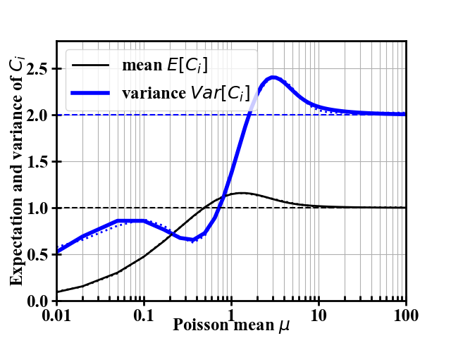
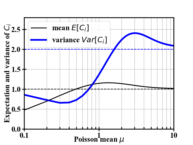
Figure 1: (Top) Expectation (in black) and variance (in blue) of each term of ${C}$ statistic, according to Equation 4. Dotted lines are the approximations of Equation 11 in the range $0.01\leq\mu\leq 100$. (Bottom) Same data as in top panel, but with more accurate best–fit models in the range $0.1\leq\mu\leq 10$.

Asymptotically, the numerical calculations reported in Figure 1 show that each term of the $C$ statistic tends to

$$\lim_{\mu\to\infty}E[C_{i}]=1,\;\lim_{\mu\to\infty}Var[C_{i}]=2$$

and therefore the asymptotic limits for the mean and variance of the $C$ statistic are

$$\lim_{\mu\to\infty}E[C]=N,\;\lim_{\mu\to\infty}Var[C]=2N,$$

which are consistent with the mean and variance of a $\chi^{2}$ distribution with a number of degrees of freedom equal to the number of measurements, $f=N$. This result is expected, since for large values of the Poisson mean, the Poisson distribution is well approximated by a Gaussian distribution of same mean and variance, and the maximum likelihood method applied to $N$ independent Gaussians of mean $S_{i}$ and variance $\sigma_{i}^{2}=S_{i}$ leads to a null–hypothesis statistic of

$$\chi^{2}=\sum_{i=1}^{N}\frac{(D_{i}-S_{i})^{2}}{S_{i}},$$ (7)

i.e., a $\chi^{2}$ distribution with $N$ degrees of freedom [5]. Moreover, Equation 3 shows that the error in approximating ${C}$ with $\chi^{2}$ is negligible for large Poisson means.

The asymptotic limit for the expectation of $C_{i}$ can also be obtained via a numerical evaluation of the expectation of $D_{i}\ln D_{i}$, assuming $D_{i}\sim\text{Poiss}(\mu)$. The expectation can be calculated via

$$E[D_{i}\ln D_{i}]=\sum_{k=0}^{\infty}k\ln k\cdot e^{-\mu}\frac{\mu^{k}}{k!},$$ (8)

which does not have a simple analytical solution. A numerical solution of this expectation as function of the Poisson mean $\mu$ is shown in Figure 2, with an asymptotic value of

$$\lim_{\mu\to\infty}E[D_{i}\ln D_{i}]=\mu\ln\mu+\frac{1}{2}.$$ (9)

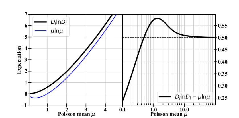
Figure 2: (Left): Expectation of function $D_{i}\ln D_{i}$ with $D_{i}\sim P(\mu)$. Notice that the function $\mu\ln\mu$ is negative for values of approximately $\mu\leq 1$ before turning positive. (Right): Expectation of $D_{i}\ln D_{i}-\mu\ln\mu$, showing the asymptotic limit of 1/2 for large $\mu$.

With this asymptotic result in hand, the asymptotic limit for the expectation of $C_{i}$ is obtained via

$$\lim_{\mu\to\infty}E[C_{i}]=\lim_{\mu\to\infty}2\cdot E[\mu-D_{i}+D_{i}\ln D_{i}-D_{i}\ln\mu]=\\ 2(\mu-\mu+\mu\ln\mu+1/2-\mu\ln\mu)=1,$$ (10)

confirming the result of Figure 1.

For convenience, the mean and variance of $C$ can be calculated using the following approximations:

$$\begin{cases}E[C_{i}]=(A+Bx+C(x-D)^{2})e^{-\alpha x}+Ee^{-\beta x}+F\\ Var[C_{i}]=(A+Bx^{2}+C(x-D)^{2})e^{-\alpha x}+(E+Fx+G(x-H)^{2})e^{-\beta x}+I.\end{cases}$$ (11)

These approximations are obtained by a fit of the curves of Figure 1 with empirical functions that were chosen to describe the two moments accurately and with just a small number of parameters. Values of the parameters $A,B,C,D,E,F,G,H,I,\alpha$ and $\beta$ are given in Table 1; one set of parameters cover the range $\mu=0.01-100$, and another set covers the range $\mu=0.1-10$ with better accuracy (see the two panels in Figure 1). For small values of the parent means, $\mu\leq 10$, the expectation and variance of ${C}$ statistic differ significantly from the asymptotic values. In particular, the expectation becomes significantly smaller than $N$ for approximately $\mu<1$. This result has implications for hypothesis testing, as discussed in the following section.

Table 1: Parameters for the functions of Equation 11.

A	B	C	D	E	F	G$\times 10^{3}$	H	I	$\alpha$	$\beta$
Parameters for $E[C_{i}]$ in range $\mu$=0.01–100
0.065672	-6.9461	-8.0124	0.40165	0.261037	1.00512	-	-	-	5.5178	0.34817
Parameters for $E[C_{i}]$ in range $\mu$=0.1–10
-0.56709	-2.7336	-2.3603	0.52816	0.33133	1.0174	-	-	-	3.9375	0.48446
Parameters for $Var[C_{i}]$ in range $\mu$=0.01–100
-2.4637	1.5109	-1.5109	0.60509	1.4761	18.358	0.87316	-0.08592	2.02343	0.62652	7.8187
Parameters for $Var[C_{i}]$ in range $\mu$=0.1–10
-3.1971	1.5118	-1.5118	0.79384	1.9294	6.1740	22.360	-7.2981	2.08378	0.750315	4.49654

3.2 Hypothesis testing with the ${C}$ statistic for a fully specified model

A discussion of hypothesis testing using the ${C}$ statistic for a fully specified model was provided in [12]. In that paper, the author correctly points out that, when there is a sufficiently large number of independent data points, typically $N\gg 10$, the central limit theorem assures that the ${C}$ statistic has an approximately normal distribution. According to the central limit theorem, the normal approximation holds true regardless of the number of counts $D_{i}$ in each independent data point, provided that the number of data points $N$ is large. The number of counts $D_{i}$, and their parent mean $\mu$, has of course an effect on the value of the mean $E[C]$ and variance $Var[C]$, as explained in Section 2.2. This large–$N$ normal approximation is not to be confused with the approximation of $C$ with a $\chi^{2}$ variable that occurs in the high–count limit, regardless of the value of $N$ (see Section 2.1).

Accordingly, in the case of a large number of data points $N$, the normal approximation to the ${C}$ statistic leads to a central confidence interval equal to

$$\left[E[C]-q\sqrt{Var[C]},E[C]+q\sqrt{Var[C]}\right].$$ (12)

The parameter $q$ takes values of, e.g., $q=1,1.7,2.6$ for, respectively, an enclosed probability $p=0.68,0.9,0.99$. Such central confidence intervals can be used to reject values of ${C}$ statistic that are too large or too small, according to the null hypothesis.

One–sided confidence intervals are often preferred by data analysists who choose to reject only large values of the fit statistic. In that case, one defines a critical value of $C$ via $p=\text{Prob}\{C\leq C_{\mathrm{crit}}\}$. When the ${C}$ statistic can be approximated as normal,

$$C_{\mathrm{crit}}=E[C]+q\sqrt{Var[C]}$$ (13)

where values $q=0.5,1.3,2.3$ can be used respectively for probabilites $p=0.68,0.9,0.99$ [see., e.g., Table A.3 of 5].

The value of the parent Poisson mean $\mu$ of each data point $D_{i}$ comes into play in finding the values of the mean $E[C]$ and variance $Var[C]$. When the Poisson mean is large, approximately $\mu\geq 10$, expressions 12 and 13 yield the same results as using a $\chi^{2}$ distribution, and tables of critical values of the $\chi^{2}$ distribution as function of $p$ and $N$ apply to the ${C}$ statistic too [e.g., Table A.3 of 5].

On the other hand, when the Poisson mean is small (approximately $\mu\leq 10$), it is necessary to use the approximations of Equation 11 into 12 and 13 to calculate confidence intervals and critical values of the ${C}$ statistic. Such confidence intervals and critical values will differ from those of a $\chi^{2}$ distribution. In particular, the critical value of the ${C}$ statistic can be substantially smaller than $N$ when $\mu\ll 1$. For example, a value of $\mu=0.5$ for $N=100$ datapoints leads to a 90% confidence value of $C_{\mathrm{crit}}\simeq 60$. For comparison, a $\chi^{2}$ distribution with the same number of degrees of freedom has a 90% critical value of $\chi^{2}_{\mathrm{crit}}=118.5$. Hypothesis testing with a fully-specified ${C}$ statistic must therefore take explicitly into account the value of the parent means of the Poisson distributions.

3.3 Expectation of ${C}_{\mathrm{min}}$ for the constant model with one free parameter

For models with free parameters, the results of Sections 3.1 and Section 3.2 are not applicable. Instead, one must take explicitly into account the fact that the fit statistic ${C}_{\mathrm{min}}$ depends on the data through the maximum likelihood method of minimization, as described in Section 2.3. The relevant statistic becomes ${C}_{\mathrm{min}}$ according to Equation 6.

The expectation of ${C}_{\mathrm{min}}$ according to Equation 6 can be re–written as

$$E[C_{\mathrm{min}}]=2N\cdot E[D_{i}\ln D_{i}]+2N\mu\ln N-2\cdot E[M\ln M].$$ (14)

where the expectation $E[D_{i}\ln D_{i}]$ and its asymptotic value were presented in Equations 8 and 9, and the expectation $E[M\ln M]$ is carried out in the same way as $E[D_{i}\ln D_{i}]$, with $M\sim\text{Poiss}(N\mu)$. The expectation of ${C}_{\mathrm{min}}$ is reported in Figure 3.

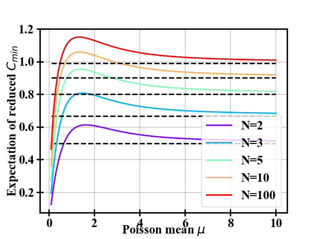
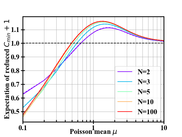
Figure 3: (Top) Expectation of ${C}_{\mathrm{min}}$ normalized by the number of variables $N$. Dashed lines are $(N-1)/N$, corresponding to the asymptotic values of $E[C_{\mathrm{min}}]=N-1$. (Bottom) Expectation of ${C}_{\mathrm{min}}$+1 divided by $N$. Asymptotic expectation for ${C}_{\mathrm{min}}$ of $N-1$ is based on $\chi^{2}_{\mathrm{min}}$ distribution with $N-1$ degrees of freedom. For $N>100$, the curves are virtually indistinguishable from the $N=100$ curve.

In the limit of large $\mu$, the expectation of ${C}_{\mathrm{min}}$ can be calculated as

$$\lim_{\mu\to\infty}E[C_{\mathrm{min}}]=2N(\mu\ln\mu+1/2)+2N\mu\ln N-2(N\mu\ln N\mu+1/2)=N-1,$$

as shown in Figure 3. This asymptotic value of $N-1$ for ${C}_{\mathrm{min}}$ is consistent with the expectation of the $\chi_{\mathrm{min}}^{2}$ distribution. In fact, for a one–parameter model, $\chi^{2}_{\mathrm{min}}$ is distributed like a $\chi^{2}$ distribution with $f=N-1$ degrees of freedom, therefore with an expectation $E[\chi^{2}_{\mathrm{min}}]=N-1$ and a variance $Var[\chi^{2}_{\mathrm{min}}]=2(N-1)$ (see, e.g., [4] and [5]). The approximation of Equation 3 also applies to models with free parameters, showing the asymptotic limit of ${C}_{\mathrm{min}}$ for one free parameter.

For small values of $\mu$, Figure 3 shows that $E[C_{\mathrm{min}}]$ can be significantly different from its asymptotic values. This result is qualitatively similar to the case of the ${C}$ statistic for a fully specified model. Expectations of the reduced ${C}_{\mathrm{min}}$+1 as function of $\mu$, and for selected values of $N$, can be accurately represented by the following empirical function in the range $0.1\leq\mu\leq 10$,

$$\dfrac{E[C_{\mathrm{min}}]+1}{N}=(A+B\mu+C(\mu-D)^{2})e^{-\alpha\mu}+Ee^{-\beta\mu}+F$$ (15)

The coefficients $A$, $B$, $C$, $D$, $E$,$F$, $\alpha$ and $\beta$ for Equation 15 are reported in Table 2.

Table 2: Model parameters for Equation 15. The $N=100$ parameters provide a good approximation also for $N>100$.

N	A	B	C	D	E	$\beta$	F	$\alpha$
2	-0.538157	0.645002	2.230719 $\times 10^{-6}$	2.44951	-0.450681	-8.10319$\times 10^{-3}$	1.50052	1.21803
3	-0.992200	0.310593	1.47508$\times 10^{-4}$	2.33858	0.314182	0.490089	1.01565	2.00042
5	-0.300655	-2.29388	-0.904818	0.970195	0.331555	0.49173111	1.01695262	3.45589169
10	-0.542826	-2.59328	-1.99152	0.590092	0.332345	0.487194	1.01733	3.81537
100	-0.600716	-2.66890	-2.360850	0.514446	0.331258	0.484436	1.017396	3.937691

3.4 Variance of ${C}_{\mathrm{min}}$ for the the constant model

The variance of ${C}_{\mathrm{min}}$ according to Equation 6 cannot be easily calculated analytically. The main challenge is that $D_{i}$ and $M$ are correlated, and therefore the expectations of the products $D_{i}\ln D_{i}\cdot M\ln M$ do not have a simple analytical form. The variance is thus estimated via a Monte Carlo simulation of Equation 6, using 10,000 samples from the $N$ Poisson variables to estimate the resulting variance of ${C}_{\mathrm{min}}$. Results of the simulations are show in Figure 4. As expected, the asymptotic value of the variance is $2(N-1)$, equal to the variance of a $\chi^{2}$ variable with $N-1$ degrees of freedom,

$$\lim_{\mu\to\infty}Var(C_{\mathrm{min}})=2(N-1).$$

The variance of ${C}_{\mathrm{min}}$ is significantly different from the asymptotic value for small values of the parent mean $\mu$, similar to the case of the mean. The variance of ${C}_{\mathrm{min}}$ can be approximated by the following formula,

$$\dfrac{Var[C_{\mathrm{min}}]}{2(N-1)}=(A+B\mu+C\mu^{2})e^{-\alpha\mu}+1.0,$$ (16)

with the parameters $A$, $B$, $C$ and $\alpha$ provided in Table 3.

Table 3: Model parameters for Equation 16. The $N=100$ parameters provide a good approximation also for $N>100$.

N	A	B	C	$\alpha$
2	-0.94444	0.38369	0.23147	0.68654
3	-0.79062	-0.12333	0.29128	0.71632
5	-0.59153	-0.54983	0.56971	0.82521
10	-0.50551	-1.0592	0.81869	0.90939
100	-0.59488	-1.0919	0.85073	0.94111

The calculations also produce sample distribution functions of ${C}_{\mathrm{min}}$. For a small number of measurements, the statistic ${C}_{\mathrm{min}}$ is necessarily skewed, given the small value of its mean and that it is positive definite, similar to the case of a $\chi^{2}$ distribution. As a result of this deviation from a normal distribution, the standard error and the half–width of a central 68% confidence interval are not the same, as also shown in Figure 4. As $N$ increases, the central limit theorem ensures that the distribution of ${C}_{\mathrm{min}}$ tends to normal, and standard error and the half–width 68% confidence intervals are in better agreement. The distribution of ${C}_{\mathrm{min}}$ is needed for hypothesis testing, as discussed in the following section.

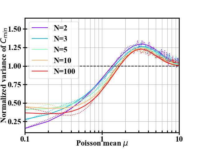
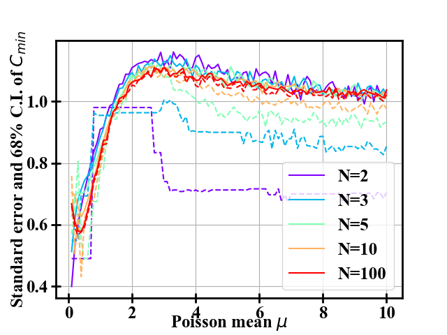
Figure 4: (Top) Variance of ${C}_{\mathrm{min}}$  normalized by $2(N-1)$. The asymptotic expectation of $2(N-1)$ is based on the $\chi^{2}_{\mathrm{min}}$ distribution for $N-1$ degrees of freedom. (Bottom) Standard deviation of ${C}_{\mathrm{min}}$ as solid curves, normalized by the same factor. Dashed curves are the half–width of central 68% confidence intervals of the normalized ${C}_{\mathrm{min}}$. Both sets of curves are normalized by the same factor $\sqrt{2(N-1)}$. For $N>100$, the curves are virtually indistinguishable from the $N=100$ curve.

3.5 Hypothesis testing and confidence intervals using ${C}_{\mathrm{min}}$

The reason to study the distribution of ${C}_{\mathrm{min}}$ beyond its mean and variance is to perform a quantitative hypothesis testing of the fit, based on $p$–values. There are two main questions that need to be addressed to test and use the results of the fit. (1) Is the value of the fit statistic ${C}_{\mathrm{min}}$ acceptable at a given probability level? (2) Assuming that the fit is acceptable, what are confidence intervals for the model parameter?

The term ‘acceptable’ is to be interpreted according to the American Statistical Association’s statement on $p$–values [15]. As is well known, $p$–values simply indicate the degree of incompatibility of a data set with a specified model, and not the probability that the hypothesis specified by the model is correct. In other words, $p$–values can only be used to reject a hypothesis or model (see also Section 7.1 of [5] for further discussion on the subject). Accordingly, a model is said to be acceptable if it cannot be rejected at a given level of probability, with the understanding that the model may or may not be the correct explanation for the data. An acceptable model is therefore simply a plausible explanation that cannot be rejected by the data at hand, at the probability specified by the $p$–value.

This section addresses both questions, also discussing the standard of practice for the use of the more popular $\chi^{2}$ statistic, and how such standard of practice can be adapted to ${C}_{\mathrm{min}}$.

3.5.1 Critical values of ${C}_{\mathrm{min}}$

The acceptability of a model (in this paper, a constant model with one parameter) can be addressed by asking whether the fit statistic ${C}_{\mathrm{min}}$ is consistent with its parent distribution based on the null hypothesis that the data are drawn from the parent model, as studied in Sections 3.3 and 3.4.

The standard of practice in many fields, including X–ray astronomy [e.g., 7], is to deem a model acceptable if the fit statistic $\chi^{2}_{\mathrm{min}}$ (for Gaussian data) has a value that is less than its critical value, defined via

$$p=\text{Prob}(\chi^{2}\leq\chi^{2}_{\mathrm{crit}}).$$

Using the probability ditribution of $\chi^{2}$, the critical values are easily evaluated (see Table A.7 of [5]). For example, a one–sided p=90% confidence interval with $f=100$ degrees of freedom has a critical value of $\chi^{2}_{\mathrm{crit}}=118.5$. Therefore, a fit with a $\chi^{2}_{\mathrm{min}}>\chi^{2}_{\mathrm{crit}}$ should be rejected at the 90% confidence level.

This method can therefore be extended to the ${C}_{\mathrm{min}}$ statistic, by calculating critical values of ${C}_{\mathrm{min}}$ at given confidence levels, defined as

$$p=\text{Prob}(C_{\mathrm{min}}\leq C_{\mathrm{min,crit}})$$

Given that the probability distribution of ${C}_{\mathrm{min}}$ is not known exactly, the calculation of critical values must be carried out by means of the same Monte Carlo simulation used to estimate the variance of ${C}_{\mathrm{min}}$. In Figure 5 are shown one–sided confidence intervals for ${C}_{\mathrm{min}}$. For comparison, equivalent confidence intervals for a $\chi^{2}$ distribution with the same number of degrees of freedom are reported in Table 4. $N$ is large, critical values can be calculated using the same method as in Equation 13, simply replacing the $C$ statistic with the ${C}_{\mathrm{min}}$ statistic, i.e.,

$$C_{\mathrm{min,crit}}=E[C_{\mathrm{min}}]+q\sqrt{Var[C_{\mathrm{min}}]}$$ (17)

where the meaning of $q$ is described in Section 3.2.

Table 4: Reference values of $\chi^{2}_{\mathrm{crit}}/f$ for selected values of the number of degrees of freedom $f$, reproduced from Table A.7 of [5]. For comparison, the model presented in this paper has $f=N-1$.

$f$	Null hypothesis probability
	0.6	0.7	0.8	0.9	0.99
1	0.71	1.07	1.64	2.71	6.63
2	0.92	1.20	1.61	2.30	4.61
4	1.01	1.22	1.50	1.95	3.32
9	1.05	1.18	1.36	1.63	2.41
100	1.03	1.07	1.12	1.19	1.38
$\infty$	1.01	1.02	1.04	1.06	1.10

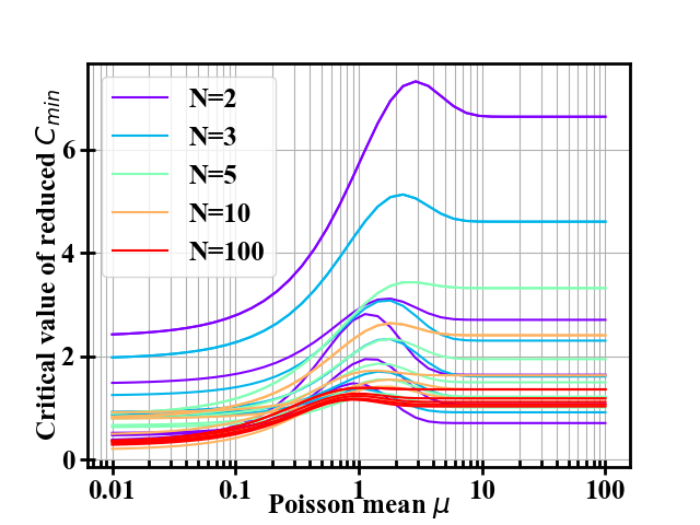
Figure 5: Critical values of one–sided confidence intervals for $C_{\mathrm{m}in}/(N-1)$ at levels of 60, 70, 80, 90 and 99% (from bottom to top, for each value of $N$).

Comparison between the values of Table 4 and those in Figure 5 show that for large values of the mean ($\mu\geq 5$), the critical value of ${C}_{\mathrm{min}}$ are very similar to those of $\chi^{2}_{\mathrm{min}}$, for all values of $N$. In this range of the parent mean, it is appropriate to use the same critical values as those of a $\chi^{2}$ distribution with the same number of degrees of freedom. For smaller values of $\mu$, critical values of ${C}_{\mathrm{min}}$ can be substantially smaller than those based on a $\chi^{2}$ distribution with the same number of degrees of freedom. In this range, one expectes substantially smaller values of ${C}_{\mathrm{min}}$ compared to $\chi^{2}_{\mathrm{min}}$, and critical values based on the latter distribution are no longer applicable to ${C}_{\mathrm{min}}$. This is an important caveat to keep in mind when analyzing Poisson data with low count rates. The results of Figure 5 only apply to the simple constant model analyzed in this paper. One–parameter models with different parameterizations, or multi–parameter models, may have different critical values, to be calculated using the appropriate formulation of ${C}_{\mathrm{min}}$ for those models. Such models are not discussed in this paper.

3.5.2 Confidence intervals on the model parameter and the $\Delta{C}$ statistic

Another key aspect of model fitting is to determine a confidence interval for the model parameters. Methods to determine confidence intervals using goodness–of–fit statistics were developed by [13], [1] and [8] using a method based on the maximum likelihood ratio theorem proposed by S. S. Wilks in 1938 [16]. For Gaussian datasets, confidence intervals on model parameters are calculated using critical values of the $\Delta\chi^{2}$ distribution. Assuming a one–parameter model as in this paper, the method is based on the observation that

$$\Delta\chi^{2}=\chi^{2}(N)-\chi^{2}_{\mathrm{min}}(N-1)$$ (18)

is distributed like a $\chi^{2}$ variable with one degree of freedom, where $N$ is the number of datapoints and $\chi^{2}_{\mathrm{min}}(N-1)$ is the usual minimum fit statistic. The $\chi^{2}(N)$ statistic assumes that the parameter is fixed at its parent (yet unknown) value, and it has no free parameters. Under the assumption that the model remains viable when the parameter value is varied from its minimum–$\chi^{2}$ value, $\Delta\chi^{2}$ is distributed as $\chi^{2}(1)$. According to Equation 18, a 68% confidence interval is therefore the range that yields $\Delta\chi^{2}\leq 1$, and a 90% confidence interval corresponds to $\Delta\chi^{2}\leq 2.7$.

For Poisson data, W. Cash [9] showed that the Wilks theorem can be used to generate confidence intervals for interesting parameters from the statistic

$$\Delta C=C-C_{\mathrm{min}},$$ (19)

which is howerer only approximately distributed like a $\chi^{2}(1)$ distribution. To calculate the exact distribution of $\Delta{C}$, one uses Equation 2 with a fixed model $S=\mu$, i.e,

$$C=2\sum_{i=1}^{N}\mu-D_{i}+D_{i}\ln\left(\frac{D_{i}}{\mu}\right),$$

as described in Section 2.2. Unlike $\Delta\chi^{2}$, it is not possible to determine exactly the distribution function for $\Delta C$ that applies to all values of $N$ and $\mu$, and therefore critical values must be estimated via Monte Carlo simulations of Equation 19 as a function of $N$ and $\mu$.

Critical values of $\Delta C$ are reported in Table 5, along with the critical values for the reference distribution $\chi^{2}(1)$. For small values of $\mu$ and $N$, the probability distribution function of $\Delta C$ and its critical values reflect the discrete nature of the Poisson distribution. For example, the probabilities to draw values $D_{i}$ of respectively 0, 1, 2 and 3 from a Poisson with mean $\mu=0.1$ are 90.5%, 9.05%, 0.45% and 0.0015%. Therefore, for $N=2$ (first entry in Table 5), most values of ${C}_{\mathrm{min}}$ are given by the following combinations of Poisson draws:

$$D_{i}=(0,0) \;C_{\mathrm{min},i}=(0,0) \;C_{i}=(0.2,0.2) \;\Delta C=0.4$$

$$D_{i}=(0,1) \;C_{\mathrm{min},i}=(0,1.4) \;C_{i}=(0.2,2.8) \;\Delta C=1.6$$

$$D_{i}=(1,1) \;C_{\mathrm{min},i}=(1.4,1.4) \;C_{i}=(2.8,2.8) \;\Delta C=2.8$$

$$D_{i}=(0,2) \;C_{\mathrm{min},i}=(0,2.8) \;C_{i}=(0.2,8.2) \;\Delta C=5.6$$

Table 5: Critical values of $\Delta C$ for selected values of the mean $\mu$. Simulations were run for 10,000 iterations for $\mu=1,10$ and for 100,000 iterations for $\mu=0.1$

$N$	Probability $p$
	0.6	0.7	0.8	0.9	0.99
$\mu$=0.1
2	0.4	0.4	0.4	1.6	5.6
3	0.6	0.6	1.0	1.0	4.2
5	1.0	1.0	1.0	1.0	5.8
10	2.0	2.0	2.0	2.0	5.1
100	0.8	1.0	1.9	3.0	6.8
$\mu$=0.3
2	1.2	1.2	1.2	2.0	4.9
3	1.8	1.8	1.8	1.8	5.7
5	1.2	1.2	3.0	3.0	5.0
10	0.4	1.1	1.8	2.3	6.0
100	0.8	1.1	1.5	2.5	6.5
$\mu$=1.0
2	0.6	0.6	1.5	4.0	5.2
3	0.4	1.1	1.8	2.3	6.0
5	0.9	0.9	1.5	2.6	7.0
10	0.8	1.0	1.9	3.0	6.8
100	0.7	1.0	1.6	2.7	6.3
$\mu$=3.0
2	0.8	0.8	1.8	2.2	6.4
3	0.9	1.1	1.6	2.4	7.0
5	0.6	1.2	1.9	2.8	7.0
10	0.8	1.1	1.8	3.0	6.7
100	0.7	1.1	1.7	2.7	6.7
$\mu$=10.0
2	0.8	1.2	1.6	2.8	7.1
3	0.8	1.1	1.8	3.0	6.5
5	0.7	1.0	1.7	2.6	6.6
10	0.7	1.0	1.6	2.7	6.7
100	0.7	1.0	1.6	2.7	6.5
	Reference $\chi^{2}(1)$
	0.71	1.07	1.64	2.71	6.63

As a result, the critical values of $\Delta C$ follow this set of discrete values. This discretization of critical values, which was not present for the $\Delta\chi^{2}$ statistic, should be taken into account when performing hypothesis testing with the $\Delta C$ statistic.

For larger values of the mean, $\mu\geq 1$, the estimates of critical values for $\Delta C$ follow closely those of a $\chi^{2}$ distribution for 1 degree of freedom. This result indicates that it is possible to treat the $\Delta C$ statistic in the same way as the $\Delta\chi^{2}$ statistic for the estimate of confidence intervals on the model parameter. Therefore, for example, a 90% confidence interval of the sample mean is obtained by finding the range of the sample mean that yield $\Delta C=2.7$, for any value of the sample size $N$.

4 Applications to X–ray data of the quasar PG 1116+215

PG 1116+215 is a quasar located at a distance from Earth of approximately 2.5 billion light years and it has been observed by the Chandra X–ray satellite several times [7, 6]. The X–ray detectors used by Chandra collect individual photons from the source and neighboring areas in the sky, and measure each photon’s wavelength. The photons are distributed in data points according to their wavelengths, and this distribution is usually referred to as the source’s spectrum.

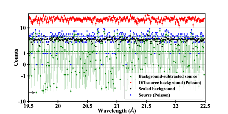
Figure 6: X–ray spectra of PG 1116+215 from an observation taken in 2018 (observation ID 19466). The off–source background (red, top data set) and the total PG 1116+215 spectrum (blue) have an integer number of counts for each data point. The scientifically interesting spectrum is the background–subtracted source spectrum (green). The point marked by an arrow and the error bars are discussed in the text. (This figure was generated in python using a symlog scaling for the $y$ axis that enables a logarithmic representation of numbers around zero.)

One of these X–ray observations is used to illustrate the application of the $C$ and ${C}_{\mathrm{min}}$ statistics to Poisson data. The top curve (red) in Figure 6 represent the spectrum collected in an off–source region of the detector that is used as a background for the source spectrum (blue). These two spectra have $N=239$ independent data points with integer counts that are modelled with a Poisson distribution, in the wavelength range of 19.5–22.5 Å.  The background spectrum is collected from a larger portion of the detector than the source area, and it is therefore re–scaled by a deterministic factor $A=0.09992$ (black data points) and then subtracted from the source spectrum to yield the background–subtracted source spectrum (green), which is the scientifically useful spectrum. Since all these spectra are approximately flat in this wavelength range, it is appropriate to model them with a constant model, using the methods described in this paper. 

4.1 The off–source background

The off–source background spectrum (Figure 6, red) has an average of over 20 counts in the $N=239$ data points. A maximum–likelihood fit of this Poisson dataset with a constant model yields a best–fit mean of $S=26.92$ for a fit statistic of ${C}_{\mathrm{min}}$=232.6, according to Equations 5 and 6. According to Figure 3, in the high–count regime ($\mu\geq 10$) the expectation of ${C}_{\mathrm{min}}$ is $N-1$, same as for a $\chi^{2}(N-1)$ distribution. Critical values of ${C}_{\mathrm{min}}$ can be calculated from the $\chi^{2}(N-1)$ distribution, which is followed closely by ${C}_{\mathrm{min}}$ in this high–count regime. Using, as an example, a $p$–value of $p=0.9$, the critical value is approximately $C_{\mathrm{min,crit}}\simeq 1.1\times(N-1)=262$, as obtained from Table A.4 of [5] or from interpolation of the values in Table 4. Since the measured value of ${C}_{\mathrm{min}}$ is lower than the critical value, the constant model is deemed acceptable at the 90% confidence level. Other $p$–values can be used following the same procedure.

In X–ray astronomy it is common to fit data with $\mu\geq 20$ counts, such as this off–source background, using the $\chi^{2}$ statistic. A $\chi^{2}$ fit with a constant model yields a best–fit mean of $25.91$, with $\chi^{2}_{\mathrm{min}}=241.34$. This $\chi^{2}$ bias towards lower values of the mean, already noted by others [e.g. 11], occurs because the $\chi^{2}$ best–fit is the weighted mean of the data points, with weights equal to $\sigma_{i}^{-2}$, instead of the sample mean (for a reference, see Chapter 8 of [5]). Since the $\chi^{2}$ statistic uses $\sigma_{i}=\sqrt{D_{i}}$ as an approximation for the standard deviations, datapoints with fewer counts have larger weight than points with higher counts, leading to a lower best–fit value. This bias can be avoided by using the ${C}_{\mathrm{min}}$ statistic, i.e., retaining the original Poisson distribution of the data, even in the large–count regime ($\mu\geq 20$).

The distribution of the $C$ statistic (and, for comparison, of $\chi^{2}$) around the minimum value of the mean is shown in Figure 7. According to the results of Section 3.5.2, we use a value of $\Delta C=2.7$ to obtain a 90% confidence interval for the mean, and report the best–fit mean level as $26.92\pm 0.54$, at the 90% confidence level. If the $\chi^{2}$ distribution had been used instead, the measurement would have been (erroneously) biased to a lower value of $25.91\pm 0.54$ (using $\Delta\chi^{2}=2.7$ for a 90% confidence interval).

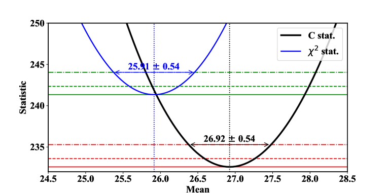
Figure 7: $C$ and $\chi^{2}$ statistics for the off–source background. The minimum values of the statistics are marked by solid horizontal lines. Dashed horizontal lines correspond to ${C}_{\mathrm{min}}$+1 and $\chi^{2}_{\mathrm{min}}+1$ (for 68% confidence intervals on $C$ and $\chi^{2}$) and dot–dashed horizontal lines to ${C}_{\mathrm{min}}$+2.7 and $\chi^{2}_{\mathrm{min}}+2.7$ (for 90% confidence).

4.2 The source spectrum

The same method of analysis is applied to the source spectrum (Figure 6, blue). The fit to a constant model returns a best–fit value of 3.85, with a fit statistic of ${C}_{\mathrm{min}}$=247.3 for $N=239$ data points. To test the null hypothesis that the constant model is viable for this spectrum, the critical value of ${C}_{\mathrm{min}}$ for $p=0.90$ is needed. Since this spectrum is in the low–count regime, it is not accurate to use Table A.4 of [5] or the values in Table 4, as was done for the off–source spectrum. Instead, one needs to use Equation 17, which is applicable to the large–$N$ case, regardless of the value of the Poisson mean. Equations 15 and 16 can be used to estimate the mean and variance of ${C}_{\mathrm{min}}$, using the coefficients that apply to the $N\geq 100$ case and for a value of $\mu=3.85$, to obtain $E[C_{\mathrm{min}}]=254.4$ and $Var[C_{\mathrm{min}}]=287.8$. With these results, the critical value for $p=0.90$ is $C_{\mathrm{min,crit}}=276.5$. Since $C_{\mathrm{min}}<C_{\mathrm{min,crit}}$, the null hypothesis cannot be rejected, and the constant model is considered acceptable. A 90% confidence interval on the best-fit mean is obtained again using the $\Delta C=2.7$ criterion, and the mean can be reported as $3.85\pm 0.22$.

4.3 The background–subtracted source spectrum

The background–subtracted spectrum is obtained by subtracting a re–scaled version of the off–source background (Section 4.1) from the source spectrum (Section 4.2). To estimate the mean level of emission, the non–Poisson nature of this spectrum prevents the direct use of a ${C}_{\mathrm{min}}$ fit to this spectrum. Instead, one may combine the results from the analysis of the two Poisson spectra, which yielded means of respectively $26.92\pm 0.54$ (prior to rescaling) and $3.85\pm 0.22$. The background–subtracted mean is therefore $3.85-A\times 26.92=1.16$, shown as a dashed green line in Figure 6. Its uncertainty can be estimated by the error propagation method (see Chapter 4 of [5]), and the background–subtracted mean can be reported as $1.16\pm 0.23$ (90% confidence).

The following illustrates how the low count rate for the source spectrum invalidates the use of $\chi^{2}$ for this background–subtracted source spectrum. The green error bars represent a Gaussian approximation for the standard deviation $\sigma_{i}$ of each background–subtracted data point, calculated according to $\sigma_{i}^{2}=(\sqrt{B_{i}}A)^{2}+D_{i}^{2}$, i.e., assuming that both background $B_{i}$ and source $D_{i}$ data are Gaussian–distributed.  This approximation is however not accurate because the $D_{i}$ data are in the low–count regime where the Poisson distribution is poorly approximated by a Gaussian. An extreme example is the data point indicated by an arrow near the bottom left of Figure 6 ($D_{i}=0$ and $B_{i}=37$), where the null contribution to the variance from $D_{i}=0$ leads to an estimated background–subtracted rate of $-3.70\pm 0.61$, with an artificially small standard deviation. As a result, using these standard deviations for a $\chi^{2}$ fit to a constant model results in a best–fit mean of -0.28 (the dashed grey line in Figure 6) that is erroneously biased low, compared to the value of $1.16\pm 0.23$ obtained earlier. The conclusion is that these low–count data should not be fit using the $\chi^{2}$ statistic, since the assumption of Gaussian data points is not accurate.

4.4 An example of Poisson data with mean $\mu<1$

A sub–set of the data of Figure 6 is used to further illustrate the application of the ${C}$ statistic to low–count data with mean $\mu<1$. Figure 8 shows the source spectrum from a 1,000–second portion of the same observation shown in Figure 6. Given the shorter observing time of this sub–set of data, the spectrum is mostly composed of 0 or 1 counts per data point, with one point having 2 counts. A fit of this data set to a constant model results in a best–fit mean of $0.100\pm 0.034$ (90% confidence interval, using $\Delta C=2.7$), for a fit statistic of ${C}_{\mathrm{min}}$=113.1. The small value of the Poisson mean resulted in a ${C}_{\mathrm{min}}$ that is substantially smaller than $N-1$. This point was illustrated by Figure 3, with $E[C_{\mathrm{cmin}}]\simeq\nicefrac{{1}}{{2}}\;N$ for $N\geq 100$ and $\mu=0.1$, instead of the asymptotic limit of $E[C_{\mathrm{cmin}}]\simeq N-1$ for large values of the Poisson mean.

The critical value of ${C}_{\mathrm{min}}$ is calculated as in Section 4.2. For a value of the Poisson mean of $\mu=0.10$ and $N=239$ data points, Equations 15 and 16 yield $E[C_{\mathrm{min}}]=112.4$ and $Var[C_{\mathrm{min}}]=85.9$, and Equation 17 gives a critical value at 90% confidence of $C_{\mathrm{min,crit}}=124.4$. Since the measured value of ${C}_{\mathrm{min}}$ is smaller than the critical value, the constant model is again acceptable for the data of Figure 8, at the 90% probability level.

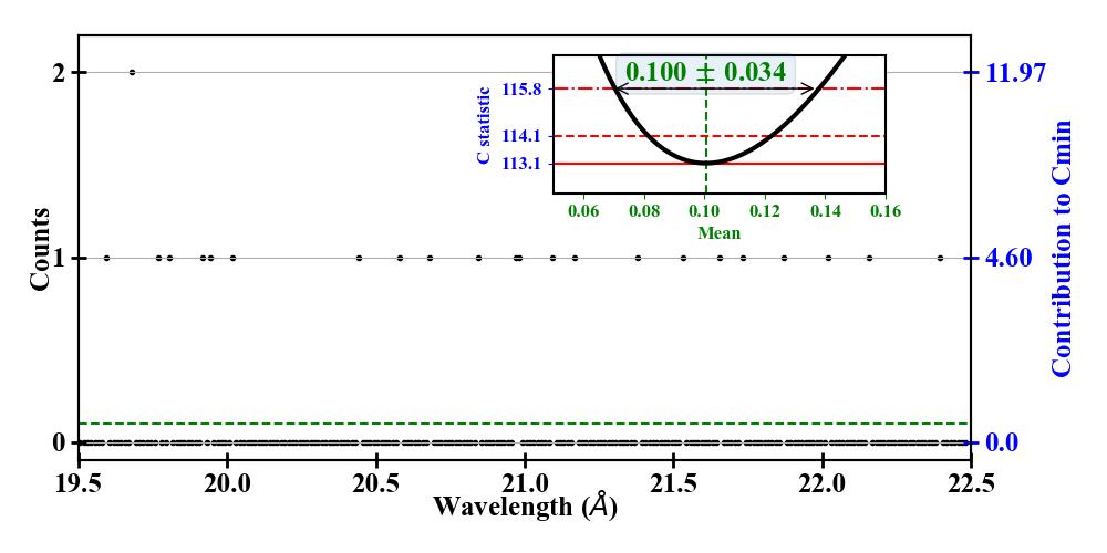
Figure 8: Spectrum of PG 1116+215 from a 1,000 second portion of the observation shown in Figure 6. Green dashed line is the mean value of 0.100 for this data set, composed mainly of points with zero or one counts. The inset shows the distribution of ${C}$ statistic around the minimum value.

The vertical axis on the right of Figure 8 shows the contribution of each data point to the ${C}_{\mathrm{min}}$ statistic. According to Equation 6, this contribution is $D_{i}\ln(D_{i}/S)$, where $S$ is the sample mean. As pointed out in Section 2.2, data points with $D_{i}=0$ counts have a null contribution to the statistic.

5 Conclusions

The ${C}$ statistic is a goodness–of–fit statistic derived from the maximum likelihood analysis of Poisson data. It is the statistic of choice to analyze low–count experiments such as astronomical spectra from faint sources. Challenges in the use of the ${C}$ statistic are associated with the unavailability of its exact probability distribution function. This paper has provided advances in our understanding of the ${C}$ statistic and of the associated statistics ${C}_{\mathrm{min}}$ and $\Delta{C}$, their applicability to data analysis, and identified avenues for future investigations.

First, in the case of a fully specified model, the asymptotic behavior of ${C}$ for a large value of the parent Poisson mean is the same as that of a $\chi^{2}$ distribution with $N$ degrees of freedom, where $N$ is the number of independent Poisson measurements. For smaller values of the Poisson mean, approximately $\mu\leq 10$, there are significant deviations from the $\chi^{2}$ distribution. In particular, for $\mu\leq 1$, the expectation of the ${C}$ statistic is significantly smaller than the corresponding $\chi^{2}$ distribution. This paper provided convenient analytical approximations for the mean and variance of the statistic.

Second, this paper investigated the effect of free model parameters by using a simple constant model with one free parameter, corresponding to the sample mean of the data. This initial effort showed that the asymptotic behavior of ${C}_{\mathrm{min}}$ is the same as that of a $\chi^{2}$ distribution with $N-1$ degrees of freedom. This result indicates that, just like in the case of the $\chi^{2}_{\mathrm{min}}$ statistic, the free parameter in the model has the effect to reduce the number of degrees of freedom by one. For small values of the Poisson mean, ${C}_{\mathrm{min}}$ can be substantially different from the corresponding $\chi^{2}_{\mathrm{min}}$ distribution, similar to the case of a fully specified model. These results have implications for hypothesis testing, whereby the statistic has substantially smaller critical values, compared to a $\chi^{2}$ distribution with $N-1$ degrees of freedom.

It was also discussed how the $\Delta C$ statistic can be used to determine confidence intervals on the model parameter, similar to the case of the $\Delta\chi^{2}$ statistic. When applied to this simple constant model, the $\Delta C$ statistic has critical values that are similar to those of $\Delta\chi^{2}$, for all $N$. The only caveat in this case is that, for $\mu\leq 1$, $\Delta C$ has only a few discrete values, unlike $\Delta\chi^{2}$, and this discretization may lead to differences between the two statistics. The indication provided by this study is that, within the uncertainties due to the discrete nature of the ${C}$ statistic, $\Delta C$ can be used in much the same way as $\Delta\chi^{2}$.

The application of these methods to observations of the quasar PG 1116+215 showed that the ${C}_{\mathrm{min}}$ statistics is to be preferred to the $\chi^{2}_{\mathrm{min}}$ statistic to fit counting (i.e., Poisson–distributed) data. In the low–count regime, the $\chi^{2}_{\mathrm{min}}$ statistic is not applicable because the data cannot be accurately approximated by a Gaussian distribution. Even in the high–count limit, the $\chi^{2}_{\mathrm{min}}$ statistic was shown to bias the constant model to lower best–fit values, compared to the ${C}_{\mathrm{min}}$ statistic. The findings of this paper therefore support the recommendation that the Poisson–based $C$ and ${C}_{\mathrm{min}}$ statistics be the statistics of choice to fit counting data, regardless of the number of counts.

The results provided in this paper may not be directly applicable to models with more than one free parameter, or for one–parameter models other than the simple constant model. An extension of this study to such models is required to ensure the applicability of these results to more complex models, in particular with regards to the result that ${C}_{\mathrm{min}}$ is significantly smaller than $\chi^{2}$ in the small–count regime. For models with $p>1$ free parameters, it is known that the asymptotic distribution of ${C}_{\mathrm{min}}$ tends to that of a $\chi^{2}$ distribution with $N-p$ number of degrees of freedom, consistent with the results of this paper. For such multi–parametric models, it is necessary to investigate further both the low–count behavior and whether the parameterization of the model has an effect of the distribution of ${C}_{\mathrm{min}}$.

References

- Avni [1976] Avni, Y. 1976, ApJ, 210, p. 642
- Baker & Cousins [1984] Baker, S., & Cousins, R. D. 1984, Nuclear Instruments and Methods in Physics Research, 221, p. 437
- Beaujean et al. [2011] Beaujean, F., Caldwell, A., Kollár, D., & Kröninger, K. 2011, Phys. Rev. D, 83, p. 012004
- Bevington & Robinson [2003] Bevington, P. R., & Robinson, D. K. 2003, Data reduction and error analysis for the physical sciences (McGraw Hill, Third Edition)
- Bonamente [2017] Bonamente, M. 2017, Statistics and Analysis of Scientific Data (Springer, Graduate Texts in Physics, Second Edition)
- Bonamente et al. [2019] Bonamente, M., Ahoranta, J., Nevalainen, J., & Holt, P. 2019, Research Notes of the AAS, 3, p. 75
- Bonamente et al. [2016] Bonamente, M., Nevalainen, J., Tilton, E., Liivamägi, J., Tempel, E., Heinämäki, P., & Fang, T. 2016, MNRAS, 457, p. 4236
- Cash [1976] Cash, W. 1976, A&A, 52, p. 307
- Cash [1979] —. 1979, ApJ, 228, p. 939
- Fruscione et al. [2006] Fruscione, A., McDowell, J. C., Allen, G. E., Brickhouse, N. S., Burke, D. J., Davis, J. E., Durham, N., Elvis, M., Galle, E. C., Harris, D. E., Huenemoerder, D. P., Houck, J. C., Ishibashi, B., Karovska, M., Nicastro, F., Noble, M. S., Nowak, M. A., Primini, F. A., Siemiginowska, A., Smith, R. K., & Wise, M. 2006, in SPIE Conference Series, Vol. 6270, 62701V
- Humphrey et al. [2009] Humphrey, P. J., Liu, W., & Buote, D. A. 2009, ApJ, 693, p. 822
- Kaastra [2017] Kaastra, J. S. 2017, A&A, 605, p. A51
- Lampton et al. [1976] Lampton, M., Margon, B., & Bowyer, S. 1976, ApJ, 208, p. 177
- Nousek & Shue [1989] Nousek, J. A., & Shue, D. R. 1989, ApJ, 342, p. 1207
- Wasserstein & Lazar [2016] Wasserstein, R. L., & Lazar, N. A. 2016, The American Statistician, 70, p. 129
- Wilks [1938] Wilks, S. S. 1938, Ann. Math. Statist., 9, p. 60