Neural-Symbolic Descriptive Action Model from Images:
The Search for STRIPS

Abstract

Recent work on Neural-Symbolic systems that learn the discrete planning model from images has opened a promising direction for expanding the scope of Automated Planning and Scheduling to the raw, noisy data. However, previous work only partially addressed this problem, utilizing the black-box neural model as the successor generator. In this work, we propose Double-Stage Action Model Acquisition (DSAMA), a system that obtains a descriptive PDDL action model with explicit preconditions and effects over the propositional variables unsupervised-learned from images. DSAMA trains a set of Random Forest rule-based classifiers and compiles them into logical formulae in PDDL. While we obtained a competitively accurate PDDL model compared to a black-box model, we observed that the resulting PDDL is too large and complex for the state-of-the-art standard planners such as Fast Downward primarily due to the PDDL-SAS+ translator bottleneck. From this negative result, we show that this translator bottleneck cannot be addressed just by using a different, existing rule-based learning method, and we point to the potential future directions.

1 Introduction

Recently, Latplan system (?) successfully connected a subsymbolic neural network (NN) system and a symbolic Classical Planning system to solve various visually presented puzzle domains. The system consists of four parts: 1) The State AutoEncoder (SAE) neural network learns a bidirectional mapping between images and propositional states with unsupervised training. 2) Action Model Acquisition module generates an action model from the propositional state transitions encoded from the images. 3) Classical Planning module solves the problem in the propositional state space with the learned action model. 4) The decoding module maps the propositional plan back to an image sequence. The proposed framework opened a promising direction for applying a variety of symbolic methods to the real world — For example, the search space generated by Latplan was shown to be compatible with a symbolic Goal Recognition system (?; ?). Several variations replacing the state encoding modules have also been proposed: Causal InfoGAN (?) uses a GAN-based framework, First-Order SAE (?) learns the First Order Logic symbols (instead of the propositional ones), and Zero-Suppressed SAE (?, ZSAE) addresses the Symbol Stability issue of the regular SAE with $\ell_{1}$ regularization.

⬇

(:action a0 :parameters () :precondition [D0]

:effect (and (when [E00] (z0))

(when (not [E00]) (not (z0)))

(when [E01] (z1))

(when (not [E01]) (not (z1))) …))

Figure 1: An example DSAMA compilation result for the first action (i.e. a0) generated from the image planning domain. [...] consists of a negation normal form compiled from a Random Forest (?, RF).

Despite these efforts, Latplan is missing a critical feature of the traditional Classical Planning systems: The use of State-of-the-Art heuristic functions. The main reason behind this limitation is the lack of descriptive action model consisting of logical formula for the preconditions and the effects, which allows the heuristics to exploit its causal structures. Obtaining the descriptive action models from the raw observations with minimal human interference is the next key milestone for expanding the Automated Planning applications to the raw unstructured inputs, as it fully unleashes the pruning power of state-of-the-art Classical Planning heuristic functions which allow the planner to scale up to much larger problems.

In this paper, we propose an approach called Dual-Stage Action Model Acquisition (DSAMA), a dual-stage process that first learns the set of action symbols and action effects via Action AutoEncoder neural network module in Latplan AMA₂ (?) and then trains a rule-based machine learning system which are then converted into propositional formula in a PDDL format. We tested DSAMA with Random Forest (RF) framework (?) as the machine learning module due to its maturity and performance. As a result, we successfully generated a descriptive action model, as depicted in Fig. 1 for example, which is as accurate as the black-box neural counterpart.

Despite the success in terms of the model accuracy, the proposed approach turned out to be an impractical solution for descriptive action model acquisition and gave us an insight into the core problem of this approach. The generated logical formula and the resulting PDDL was too large and complex for the recipient classical planning system (Fast Downward) to solve the given instance in a reasonable runtime and memory, and if we trade the accuracy with the model simplicity, the goal becomes unreachable. We provide an analysis on the reason and discuss possible future directions. The code reproducing the experiments will be published at github.com/guicho271828/latplan/.

2 Preliminaries

We denote a tensor (multi-dimensional array) in bold and denote its elements with a subscript, e.g. when ${\bm{x}}\in\mathbb{R}^{N\times M}$, the second row is ${\bm{x}}_{2}\in\mathbb{R}^{M}$. We use dotted subscripts to denote a subarray, e.g. ${\bm{x}}_{2..5}=({\bm{x}}_{2},{\bm{x}}_{3},{\bm{x}}_{4})$. For a vector or a set $X$, $|X|$ denotes the number of elements. $\bm{1}^{D}$ and $\bm{0}^{D}$ denote the constant matrix of shape $D$ with all elements being 1/0, respectively. ${\bm{a}};{\bm{b}}$ denotes a concatenation of tensors ${\bm{a}}$ and ${\bm{b}}$ in the first axis where the rest of the dimensions are same between ${\bm{a}}$ and ${\bm{b}}$. For a dataset, we generally denote its $i$-th data point with a superscript ⁱ which we may sometimes omit for clarity.

Let $\mathcal{F}(V)$ be a propositional formula consisting of logical operations ${\left\{\land,\lor,\lnot\right\}}$, constants ${\left\{\top,\bot\right\}}$, and a set of propositional variables $V$. We define a grounded (propositional) Classical Planning problem as a 4-tuple ${\left<P,A,I,G\right>}$ where $P$ is a set of propositions, $A$ is a set of actions, $I\subset P$ is the initial state, and $G\subset P$ is a goal condition. Each action $a\in A$ is a 3-tuple ${\left<\textsc{pre}{\left(a\right)},\textsc{eff}^{+}{\left(a\right)},\textsc{eff}^{-}{\left(a\right)}\right>}$ where $\textsc{pre}{\left(a\right)}\in\mathcal{F}(P)$ is a precondition and $\textsc{eff}^{+}{\left(a\right)}$, $\textsc{eff}^{-}{\left(a\right)}$ are the sets of effects called add-effects and delete-effects, respectively. Each effect is denoted as $c\triangleright e$ where $c\in\mathcal{F}(P)$ is an effect condition and $e\in P$. A state $s\subseteq P$ is a set of true propositions, an action $a$ is applicable when $s\vDash\textsc{pre}{\left(a\right)}$ ($s$ satisfies $\textsc{pre}{\left(a\right)}$), and applying an action $a$ to $s$ yields a new successor state $a(s)$ which is $a(s)=s\cup{\left\{e\mid(c\triangleright e)\in\textsc{eff}^{+}{\left(a\right)},c\vDash s\right\}}\setminus{\left\{e\mid(c\triangleright e)\in\textsc{eff}^{-}{\left(a\right)},c\vDash s\right\}}$.

Modern classical planners such as Fast Downward (?) takes the PDDL (?) input which specifies the above planning problem, and returns an action sequence that reaches the goal state from the initial state. Recent planners typically convert a propositional planning model into SAS+ (?) format, upon which the disjunctions in the action model must be eliminated by moving the disjunctions to the root of the formula and splitting the actions (?).

Latplan

Latplan (?) is a framework for domain-independent image-based classical planning. It learns the state representation as well as the transition rules entirely from the image-based observation of the environment with deep neural networks and solves the problem using a classical planner.

Latplan takes two inputs. The first input is the transition input Tr, a set of pairs of raw data randomly sampled from the environment. An $i$-th data pair in the dataset $\text{tr}^{i}=({\bm{x}}^{i,0},{\bm{x}}^{i,1})\in\text{Tr}$ represents a randomly sampled transition from an environment observation ${\bm{x}}^{i,0}$ to another observation ${\bm{x}}^{i,1}$ where some unknown action took place. The second input is the planning input $({{\bm{x}}^{I}},{{\bm{x}}^{G}})$, a pair of raw data, which corresponds to the initial and the goal state of the environment. The output of Latplan is a data sequence representing the plan execution $({{\bm{x}}^{I}},\ldots{{\bm{x}}^{G}})$ that reaches ${{\bm{x}}^{G}}$ from ${{\bm{x}}^{I}}$. While the original paper used an image-based implementation (“data” = raw images), the type of data is arbitrary as long as it is compatible with neural networks.

Latplan works in 3 steps. In Step 1, a State AutoEncoder (SAE) (Fig. 2, left) neural network learns a bidirectional mapping between raw data ${\bm{x}}$ (e.g., images) and propositional states ${\bm{z}}\in{\left\{0,1\right\}}^{F}$, where the propositional states are represented by $F$-dimensional bit vector. The network consists of two functions Encode and Decode, where Encode maps an image ${\bm{x}}$ to ${\bm{z}}=\textsc{Encode}({\bm{x}})$, and Decode function maps ${\bm{z}}$ back to an image ${\bm{y}}=\textsc{Decode}({\bm{z}})$. The training is performed by minimizing the reconstruction loss $||{\bm{y}}-{\bm{x}}||$ under some norm (e.g., Mean Square Error for images). In order to guarantee that ${\bm{z}}$ is a binary vector, the network must use a discrete latent representation learning method such as Gumbel Softmax (?; ?) or Step Function with straight-through estimator (?; ?) — We used Gumbel Softmax annealing-based continuous relaxation $\textsc{GumbelSoftmax}({\bm{x}})=\textsc{Softmax}(({\bm{x}}-\log(-\log(\textsc{Uniform}(0,1))))/\tau)$, $\tau\rightarrow 0$ in this paper. After learning the mapping from ${\left\{\ldots{\bm{x}}^{i,0},{\bm{x}}^{i,1}\ldots\right\}}$, SAE obtains the propositional transitions $\overline{\text{Tr}}=$ ${\left\{(\textsc{Encode}({\bm{x}}^{i,0}),\textsc{Encode}({\bm{x}}^{i,1}))\right\}}={\left\{({\bm{z}}^{i,0},{\bm{z}}^{i,1})\right\}}$. In Step 2, an Action Model Acquisition (AMA) method learns an action model from $\overline{\text{Tr}}$. In Step 3, a planning problem instance is generated from the planning input $({{\bm{x}}^{I}},{{\bm{x}}^{G}})$. These are converted to the discrete states $({{\bm{z}}^{I}},{{\bm{z}}^{G}})$ and the classical planner finds the path connecting them. For example, an 8-puzzle problem instance consists of an image of the start (scrambled) configuration of the puzzle and an image of the solved state. In the final step, Latplan obtains a step-by-step, human-comprehensive visualization of the plan execution by Decode’ing the latent bit vectors for each intermediate state and validates the visualized result using a custom domain-specific validator, for the evaluation purpose. This is because the SAE-generated latent bit vectors are learned unsupervised and not directly verifiable through human knowledge.

Action Model Acquisition (AMA)

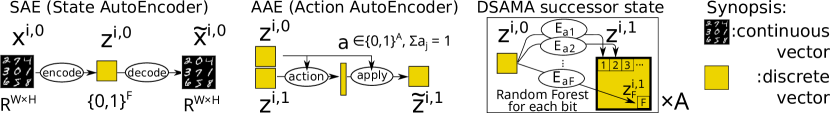
Figure 2: The illustration of State AutoEncoder, Action AutoEncoder, and Double Stage AMA for effect prediction.

The original Latplan paper proposed two approaches for AMA. AMA₁ is an oracular model that directly generates a PDDL without learning, and AMA₂ is a neural model that approximates AMA₁ by learning from examples.

AMA₁ is an oracular, idealistic AMA that does not incorporate machine learning, and instead generates the entire propositional state transitions from the entire image transitions in the search space. Each propositional transition is turned into a single, grounded action schema. For example, in a state space represented by 2 latent space propositions ${\bm{z}}=({\bm{z}}_{1},{\bm{z}}_{2})$, a transition from ${\bm{z}}^{i,0}=(0,1)$ to ${\bm{z}}^{i,1}=(1,0)$ is translated into an action with $\textsc{pre}{\left(a\right)}=\lnot{\bm{z}}_{1}\land{\bm{z}}_{2},\textsc{eff}^{+}{\left(a\right)}={\left\{\top\triangleright{\bm{z}}_{1}\right\}},\textsc{eff}^{-}{\left(a\right)}={\left\{\top\triangleright{\bm{z}}_{2}\right\}}$. It is impractical because it requires the entire image transitions, but also because the size of the PDDL is proportional to the number of transitions in the state space, slowing down the PDDL-SAS+ translation, preprocessing, and heuristic calculation at each search node.

AMA₂ consists of two neural networks: Action AutoEncoder (AAE) and Action Discriminator (AD). AAE is an autoencoder that learns to cluster the state transitions into a (preset) finite number of action labels. See Fig. 2 (middle) for the illustration.

AAE’s encoder takes a propositional state pair $({\bm{z}}^{i,0},{\bm{z}}^{i,1})$ as the input. The last layer of the encoder is activated by a discrete activation function (such as Gumbel Softmax) to become a one-hot vector of $A$ categories, ${\bm{a}}^{i}\in{\left\{0,1\right\}}^{A}$ ($\sum_{1\leq j\leq A}{\bm{a}}^{i}_{j}=1$), where $A$ is a hyperparameter for the maximum number of action labels and ${\bm{a}}^{i}$ represents an action label. For clarity, we use the one-hot vector ${\bm{a}}^{i}$ and the index $a^{i}=\arg\max{\bm{a}}^{i}$ interchangeably. AAE’s decoder takes the current state ${\bm{z}}^{i,0}$ and ${\bm{a}}^{i}$ as the input and output $\tilde{{\bm{z}}}^{i,1}$, which is a reconstruction of ${\bm{z}}^{i,1}$. The encoder $\textsc{action}({\bm{z}}^{i,0},{\bm{z}}^{i,1})={\bm{a}}^{i}$ acts as a function that tells “what action has happened” and the decoder can be seen as a progression function $\textsc{apply}({\bm{a}}^{i},{\bm{z}}^{i,0})=\tilde{{\bm{z}}}^{i,1}$ (Fig. 2, middle).

AD is a binary classifier that models the preconditions of the actions. AD learns the condition from the observed propositional state transitions $\overline{\text{Tr}}$ and a “fake” state transitions. Let $P=\overline{\text{Tr}}$ and $U$ be the fake transitions. $U$ could be generated by applying a random action $1\leq a\leq A$ to the states in $\overline{\text{Tr}}$.

This learning task is a Positive-Unlabeled learning task (?, PU-learning). While all examples in $P$ are guaranteed to be the positive (valid) examples obtained from the observations, the examples in $U$ are unlabeled, i.e., we cannot guarantee that the examples in $U$ are always negative (invalid). Unlike the standard binary classification task, which takes the purely positive and the purely negative dataset, PU-learning takes such a positive and an unlabeled dataset and returns a positive-negative classifier. Under the assumption that the positive examples are i.i.d.-sampled from the entire distribution of positive examples, one can obtain a positive-negative classifier $D({\bm{s}})$ for the input ${\bm{s}}$ by correcting the confidence value of a labeled-unlabeled classifier $D_{PU}({\bm{s}})$ by an equation $D({\bm{s}})=D_{PU}({\bm{s}})/c(V_{P})$, where $V_{P}$ is a positive validation set and $c(V_{P})=\mathbb{E}_{{\bm{s}}\in V_{P}}\left[D_{PU}({\bm{s}})\right]$ is a constant computed after the training of $D_{PU}({\bm{s}})$ (?). In AD, ${\bm{s}}$ is $({\bm{z}}^{i,0};{\bm{z}}^{i,1})$, i.e., the concatenation of the propositional current state and the successor state, unlike the standard STRIPS setting where the precondition only sees the current state.

Combining AAE and AD yields a successor function that can be used for graph search algorithms: It first enumerates the potential successor states from the current state ${\bm{z}}$ by iterating ${\bm{z}}^{a}=\textit{apply}({\bm{z}},{\bm{a}})$ over $1\leq a\leq A$, then prunes the generated successor states using AD, i.e., whether $D({\bm{z}};{\bm{z}}^{a})>0.5$. The major drawback of this approach is that both AAE and AD are black-box neural networks, and thus are incompatible with the standard PDDL-based planners and heuristics, and requires a custom heuristic graph search solver.

3 Double-Stage Learning

To overcome the lack of PDDL compatibility of the black-box NNs in AMA₂, we propose Double-Stage Action Model Acquisition method (DSAMA) which consists of 3 steps: (1) It trains the same AAE networks to identify actions and perform the clustering, (2) transfers the knowledge to a set of Random Forest binary classifiers (Fig. 2, right), then finally (3) converts the classifiers into logical preconditions / effects in PDDL. Let $M$ be a process that returns a Random Forest binary classifier and let $\textsc{toPDDL}(b)$ be a function that converts a classifier $b$ into a logical formula $\overline{b}$. The overall DSAMA process is shown in Algorithm 1.

Algorithm 1 Double-Stage Action Model Acquisition for $\overline{\text{Tr}}$ with a Random Forest classifier $M$.

Perform AAE training on $\overline{\text{Tr}}$ and obtain action function.

for all $1\leq a\leq A$ do

    $Z^{0}_{a}\leftarrow{\left\{{\bm{z}}^{i,0}|({\bm{z}}^{i,0},{\bm{z}}^{i,1})\in\overline{\text{Tr}},\textsc{action}({\bm{z}}^{i,0},{\bm{z}}^{i,1})=a\right\}}$

    $Z^{1}_{a}\leftarrow{\left\{{\bm{z}}^{i,1}|({\bm{z}}^{i,0},{\bm{z}}^{i,1})\in\overline{\text{Tr}},\textsc{action}({\bm{z}}^{i,0},{\bm{z}}^{i,1})=a\right\}}$

    $Z_{a}\leftarrow{\left\{{\bm{z}}^{i,0};{\bm{z}}^{i,1}|({\bm{z}}^{i,0},{\bm{z}}^{i,1})\in\overline{\text{Tr}},\textsc{action}({\bm{z}}^{i,0},{\bm{z}}^{i,1})=a\right\}}$

    $U_{a}\leftarrow{\left\{{\bm{z}}^{i,0};{\bm{z}}^{i,1}|({\bm{z}}^{i,0},{\bm{z}}^{i,1})\in\overline{\text{Tr}},\textsc{action}({\bm{z}}^{i,0},{\bm{z}}^{i,1})\not=a\right\}}$

    for all $1\leq f\leq F$ do

        $Z^{1}_{af}\leftarrow{\left\{{\bm{z}}_{f}|{\bm{z}}\in Z^{1}_{a}\right\}}$

        $E_{af}\leftarrow M(Z^{0}_{a},Z^{1}_{af})$

        $\overline{E}_{af}\leftarrow\textsc{toPDDL}(E_{af})$ (Effect conditions for ${\bm{z}}_{f}$)     

    $D_{a}\leftarrow M((Z_{a};U_{a}),\;(\bm{1}^{|Z_{a}|};\bm{0}^{|U_{a}|}))$ ($(X;Y)=$ concat of $X$ and $Y$)

    $\overline{D}_{a}\leftarrow\textsc{toPDDL}(D_{a})$ (precondition)

    collect action ${\left<\overline{D}_{a},\ \bigcup_{f}{\left\{\overline{E}_{af}\triangleright{\bm{z}}_{f}\right\}},\ \bigcup_{f}{\left\{\lnot\overline{E}_{af}\triangleright\lnot{\bm{z}}_{f}\right\}}\right>}$.

In order to learn the action preconditions, DSAMA performs a PU-learning following Action Discriminator (Sec. 2). Similar to AD, it takes both the current and successor states as the input – in the later experiments, we show that the accuracy drops when we limit the input to the current state. Unlike AD in AMA₂, DSAMA trains a specific classifier for each action. For the action effects, DSAMA learns the effect condition $c$ of the conditional effect $c\triangleright e$ in PDDL (Sec. 2). DSAMA iterates over every action $a$ and every bit $f$ and trains a binary classifier $E_{af}$ that translates to $c$.

Random Forest (RF)

While the binary classifier in DSAMA could be any binary classifier that could be converted to a logical formula, we chose Random Forest (?), a machine learning method based on decision trees. It constructs an ensemble of decision trees ${\bm{t}}={\left({\bm{t}}_{1}\ldots{\bm{t}}_{T}\right)}$ and averages the predictions returned by each tree ${\bm{t}}_{i}$. We do not describe the details of its training, which is beyond the scope of this paper. It is one of the most widely used rule-based learning algorithms whose implementations are available in various machine learning packages . To address the potential data imbalance, we used a Balanced Random Forest algorithm (?).

A decision tree for classification consists of decision nodes and leaf nodes. A decision node is a 4-tuple $(i,\theta,\textit{left},\textit{right})$, where each element is the feature index, a threshold, and the left / right child nodes. A leaf node contains a class probability vector ${\bm{p}}\in[0,1]^{C}$, where $C$ is a number of classes to be classified, which is 2 in our binary case. To classify a feature vector ${\bm{x}}\in\mathbb{R}^{F}$, where $F$ is the number of features, it tests ${\bm{x}}_{i}\leq\theta$ at each decision node and recurses into the left/right children depending on success. When a single tree is used for classification, it takes the $\operatorname*{arg\,max}$ over the probability vector at the leaf node and returns the result as the predicted classification. For an ensemble of decision trees, classification is performed either by taking the average of ${\bm{p}}$ returned by the trees and then taking an $\operatorname*{arg\,max}$ over the classes, or by taking the $\operatorname*{arg\,max}$ at each leaf node and returning the majority class voted by each tree.

Since STRIPS/PDDL cannot directly represent the numeric averaging operation, we simulate the voting-based inference of Random Forest in the PDDL framework by compiling the RF into a majority gate boolean circuit.

First, converting a decision tree into a boolean logic formula is straightforward. Since we assume a binary input dataset, the decision nodes and the leaf nodes can be recursively converted into a Negation Normal Form as in the toPDDL(tree $t$) method (Algorithm 2).

Next, recall that we now take the votes from all trees and choose the class with the largest votes as the final classification prediction. Since we are handling the binary classification, finding the most voted class is equivalent to computing a majority function (?), a boolean function of $T$ fan-ins and a single fan-out which returns 1 when more than $\lfloor T/2\rfloor$ inputs are 1. One practical approach for implementing such a function is based on bitonic sorting network (?; ?). First, we apply the bitonic sorting algorithm proposed by ? (Algorithm 2) to ${\bm{t}}_{i}$, except that instead of taking the $\max$ and $\min$ in the compareAndSwap function, we take $\lor$ and $\land$ of the elements being swapped because $\max(x,y)=x\lor y$ and $\min(x,y)=x\land y$ for 0/1 values seen as boolean values. We then use the $\lfloor T/2\rfloor$-th element stored in the result as the output. See examples in Fig. 3, Fig. 4, Fig. 1.

Finally, since our preconditions $D_{a}$ takes the current and the successor states as the input, we need to take care of the decision nodes that points to the successor state. When the binary latent space has $F$ dimensions, the input vector to the random forest has $2F$ dimensions where the first and the second half of $2F$ dimensions is for the current and the successor state. In toPDDL, when the index $i$ of the decision node satisfies $F<i$, we insert $\overline{E}_{a(i-F)}$ instead of ${\bm{z}}_{i}$ because our DSAMA formulation guarantees that ${\bm{z}}_{i}$ is true in the successor bit when the effect condition $\overline{E}_{a(i-F)}$ is satisfied. This can be seen as a trick to implement a one-step lookahead in the action model.

Algorithm 2 toPDDL method for Random Forest (?) based on bitonic sorting network (?)

function toPDDL(forest ${\bm{t}}={\left({\bm{t}}_{1}\ldots{\bm{t}}_{T}\right)}$)

    $\textsc{sort}(\top,{\bm{t}})$ $\triangleright$ Bitonic sorting

    return ${\bm{t}}_{\lfloor T/2\rfloor}$

function toPDDL(tree $t$)

    if $t$ is a decision node $(i,\theta,\textit{left},\textit{right})$ then

        if $0<\theta<1$ then

            return $({\bm{x}}_{i}\land\textsc{toPDDL}(\textit{left}))\lor(\lnot{\bm{x}}_{i}\land\textsc{toPDDL}(\textit{right}))$         

        if $\theta<0$ return $\textsc{toPDDL}(\textit{right})$, else return $\textsc{toPDDL}(\textit{left})$

    else if $t$ is a leaf node $(p_{0},p_{1})$ then

        if $p_{0}<p_{1}$ return $\top$, else return $\bot$     

function sort(bool $u$, vector ${\bm{x}}$)

    if $|{\bm{x}}|\leq 1$ then return ${\bm{x}}$

    else$\triangleright$ Note: $({\bm{a}};{\bm{b}})$ is a concatenation of vector ${\bm{a}}$ and ${\bm{b}}$ (Sec. 2).

        $d\leftarrow\lfloor|{\bm{x}}|/2\rfloor,\quad{\bm{a}}\leftarrow{\bm{x}}_{0..d},\quad{\bm{b}}\leftarrow{\bm{x}}_{d..|{\bm{x}}|}$

        return $\textsc{merge}(u,(\textsc{sort}(\top,{\bm{a}});\textsc{sort}(\bot,{\bm{b}}))))$     

function merge(bool $u$, vector ${\bm{x}}$)

    if $|{\bm{x}}|\leq 1$ then return ${\bm{x}}$

    else

        $\textsc{compareAndSwap}(u,{\bm{x}})$

        $d\leftarrow\lfloor|{\bm{x}}|/2\rfloor,\quad{\bm{a}}\leftarrow{\bm{x}}_{0..d},\quad{\bm{b}}\leftarrow{\bm{x}}_{d..|{\bm{x}}|}$

        return $(\textsc{merge}(u,{\bm{a}});\textsc{merge}(u,{\bm{b}}))$     

function compareAndSwap(bool $u$, vector ${\bm{x}}$)

    $d\leftarrow\lfloor|{\bm{x}}|/2\rfloor$

    for all $i\in{\left\{0..d\right\}}$ do

        if $u$ then $\triangleright$ Compare in increasing order?

            ${\bm{x}}_{i}\leftarrow{\bm{x}}_{i}\lor{\bm{x}}_{i+d}$ $\triangleright$ originally $\max({\bm{x}}_{i},{\bm{x}}_{i+d})$

            ${\bm{x}}_{i+d}\leftarrow{\bm{x}}_{i}\land{\bm{x}}_{i+d}$ $\triangleright$ $\min({\bm{x}}_{i},{\bm{x}}_{i+d})$

        else

            ${\bm{x}}_{i}\leftarrow{\bm{x}}_{i}\land{\bm{x}}_{i+d}$ $\triangleright$ $\min({\bm{x}}_{i},{\bm{x}}_{i+d})$

            ${\bm{x}}_{i+d}\leftarrow{\bm{x}}_{i}\lor{\bm{x}}_{i+d}$ $\triangleright$ $\max({\bm{x}}_{i},{\bm{x}}_{i+d})$             

Figure 3: Majority-gate implementation for 4 inputs $p_{0}\ldots p_{3}$, using 7 comparators $d_{0}\ldots d_{6}$ generated as part of bitonic sorting network.

Figure 4: Compilation of a decision tree into a logical formula in PDDL (as a precondition or an effect condition).

4 Evaluation

We evaluated our approach in the dataset used by ?, which consists of 5 image-based domains. MNIST 8-puzzle is an image-based version of the 8-puzzle, where tiles contain hand-written digits (0-9) from the MNIST database (?). Valid moves in this domain swap the “0” tile with a neighboring tile, i.e., the “0” serves as the “blank” tile in the classic 8-puzzle. The Scrambled Photograph 8-puzzle (Mandrill, Spider) cuts and scrambles real photographs, similar to the puzzles sold in stores). These differ from the MNIST 8-puzzle in that “tiles” are not cleanly separated by black regions (we re-emphasize that Latplan has no built-in notion of square or movable region). LightsOut is a video game where a 4x4 grid of lights is in some on/off configuration, and pressing a light toggles its state as well as the states of its neighbors. The goal is all lights Off. Twisted LightsOut distorts the original LightsOut game image by a swirl effect, showing that Latplan is not limited to handling rectangular “objects”/regions. In all domains, we used 9000 transitions for training and 1000 transitions for testing. Note that 8-puzzle contains 362880 states and 967680 transitions, and LightsOut contains 65536 states and 1048576 transitions.

We used the SAE with $F=100$, i.e., it produces 100 latent propositions. Following the work of (?), we used the standard version of SAE and a regularized version of SAE (ZSAE) with a regularization constant $\alpha=0.5$. For the AAE, we tuned the upper-bound $A$ of the number of actions in AAE by iteratively increasing $A$ from $A=8$ to $A=128$ by $\Delta A=8$ until the mean absolute error of AAE ($|{\bm{z}}^{i,1}-\tilde{{\bm{z}}}^{i,1}|$) goes below 0.01, i.e., below 1 bit on average. This is because a large $A$ reduces the number of transitions that fall into a single action label and makes the random forest training harder due to the lack of examples.

4.1 Accuracy

We compared the accuracy of DSAMA and AMA₂. DSAMA has two primary controlling hyperparameters for Random Forest — the maximum depth of the tree and the number of trees. Other hyperparameters of Random Forest follows the standard parameters for classification tasks: Entropy-based variable selection, out-of-bag ratio 0.33 (each decision tree is trained on the random $\frac{2}{3}$ subset of the entire dataset), and the number of variables considered by each tree as $\sqrt{F}$ for the $F$-dimensional dataset. (note: this is not equivalent to the tree depth because the same variable may be selected several times.)

We first compared the successor generation accuracy between AAE (black-box NN model) and DSAMA. The dataset $\overline{\text{Tr}}$ is divided into the training set and the test set by 9:1. AAE uses the same hyperparameters used in Latplan (?). DSAMA uses a Random Forest with the number of trees $T=80$ and the maximum depth of the tree $D=100$, the largest number we used in this paper. Note that, in general, Random Forest is claimed to achieve the monotonically higher accuracy as it has more ensembles and depth. Table 1 shows the average reconstruction accuracy for the successor states over $F$ bits, over all transitions in the test dataset. The results indicate that DSAMA based on Random Forest is competitive against the black box neural model.

Next, we compared the F-measure based on the true positive rate (=recall) and the true negative rate (=specificity) of the black-box precondition model (Action Discriminator) and the DSAMA precondition model using Random Forest. Note that this task is not only a PU-learning task, but also a classification task on a potentially highly imbalanced dataset and therefore we cannot use the accuracy as the evaluation metric as it could be skewed toward the majority dataset (?).

Similar results are obtained in Table 2: Rule-based method (Random-Forest) is competitive against the black box method when a sufficiently large capacity is provided to the model ($T=80,D=100$). To address the concern about using the successor states as part of the precondition, we also tested the variants which learns only from the current state. We observed a significant drop in the accuracy both in the black-box NN (AD) and the DSAMA $D_{a}$.

SAE AMA₂ AAE DSAMA $E_{af}$ Domain $\alpha$ MSE $A$ Successor bit accuracy LOut 0.0 2.25E-12 37 99.1% 98.5% LOut 0.5 8.18E-11 43 99.4% 99.2% Twisted 0.0 1.03E-02 48 99.3% 98.8% Twisted 0.5 1.08E-02 39 98.8% 98.4% Mandrill 0.0 7.14E-03 14 99.9% 98.9% Mandrill 0.5 7.09E-03 9 99.4% 98.9% Mnist 0.0 3.34E-04 67 98.8% 94.0% Mnist 0.5 3.44E-03 3 99.8% 99.5% Spider 0.0 9.51E-03 9 99.2% 98.5% Spider 0.5 8.88E-03 8 99.5% 98.4%

Table 1: Accuracy comparison between AAE and DSAMA on the successor state prediction task, where the discrete transitions are generated by the SAE or ZSAE ($\alpha=0.5$) for 5 domains. The accuracy is measured by the number of bits correctly predicted by the model in the test dataset. DSAMA uses a Random Forest with the number of trees $T=80$ and the maximum depth of the tree $D=100$. We observed that the Random Forest is competitive for this task against a black box NN and sometimes even outperformed it. As a reference, we also showed: (1) $A$, the number of action labels generated by the AAE, and (2) the image reconstruction error of the SAE, where the values are MSE for the pixel values in $[0,1]\subset\mathbb{R}$.

AMA₂ AD DSAMA $D_{a}$ Input dataset $\rightarrow$ $\overline{\text{Tr}}$ ${\left\{({\bm{z}}^{i,0};{\bm{a}}^{i})\right\}}$ $Z_{a}$ $Z^{0}_{a}$ LOut $\alpha=$0.0 89.7% 74.2% 81.5% 75.0% LOut 0.5 89.1% 68.7% 85.5% 71.7% Twisted 0.0 84.3% 75.5% 80.3% 71.5% Twisted 0.5 84.5% 72.6% 78.8% 69.6% Mandrill 0.0 81.6% 76.2% 82.4% 76.5% Mandrill 0.5 66.0% 29.1% 77.2% 59.6% Mnist 0.0 87.5% 81.6% 84.4% 78.2% Mnist 0.5 63.8% 57.0% 61.6% 57.5% Spider 0.0 82.5% 64.3% 80.7% 69.2% Spider 0.5 60.1% 15.9% 77.9% 68.3%

Table 2: F-measure of true positive rate (recall) and true negative rate (specificity), comparing AD and DSAMA on the action applicability task. The discrete transitions are generated by the SAE or ZSAE ($\alpha=0.5$) for 5 domains. Given the prediction $X$ and the ground truth $G$, $\text{recall}=P(X=1\mid G=1)$, $\text{specificity}=P(X=0\mid G=0)$, and $\text{F}=\frac{2\cdot\text{recall}\cdot\text{specificity}}{\text{recall}+\text{specificity}}$. The numbers are for a test dataset where each transition is assigned a boolean ground-truth value by a validator that works on the reconstructed image pairs. DSAMA uses a Random Forest with the number of trees $T=80$ and the maximum depth of the tree $D=100$. We show the results with the current state as the input, and those with the concatenation of the current and the successor states as the input. The accuracy drops when the input dataset is limited to the current state only.

Next, in order to see the effect of the random forest hyperparameters on the learned results, we performed an exhaustive experiment on $(T,D)\in{\left\{1,2,5,10,20,40,80\right\}}\times{\left\{4,7,12,25,50,100\right\}}$ and compared the precondition accuracy, the effect accuracy and the size of the PDDL files. Note that $T=1$ is a degenerative case for a single decision tree without ensembles. For the space constraint, we only show the results for Mandrill 8-Puzzle with ZSAE ($\alpha=0.5$), but the overall characteristics were the same across domains and the choice of SAE / ZSAE.

We observed that the effect of larger $T$ and $D$ saturates quickly, while small numbers negatively affect the performance. The action applicability prediction (i.e., the precondition accuracy, Table 3, left) tends to be more affected by the depth $D$ while the successor state reconstruction accuracy (i.e., the effect accuracy, Table 3, middle) tends to be more affected by the number of trees $T$. Larger $T$ and $D$ also implies larger file sizes. (Note: When generating the PDDL file, we apply De-Morgan’s law to simplify obvious invariants when one is encountered, e.g., $v\land\top=v$, $v\lor\bot=v$, $v\land\lnot v=\bot$ and $v\lor\lnot v=\top$.)

$T$ 1 2 5 10 20 40 80 Action applicability (precondition) F-measure $D$ 4 7 12 25 50 100 36.5% 56.1% 65.5% 49.2% 49.8% 49.5% 40.5% 59.1% 67.0% 63.8% 63.8% 64.0% 37.3% 56.8% 70.1% 69.0% 69.5% 68.8% 35.7% 56.2% 71.1% 72.7% 72.9% 72.5% 35.9% 56.8% 72.4% 75.0% 74.8% 74.6% 32.8% 55.6% 73.1% 76.6% 76.2% 76.4% 33.4% 55.6% 73.1% 77.1% 77.1% 77.2% Successor state reconstruction (effect) accuracy $D$ 4 7 12 25 50 100 87.7% 90.6% 91.7% 91.8% 91.8% 91.8% 91.5% 93.0% 91.8% 91.9% 91.9% 91.9% 94.4% 95.8% 96.3% 96.3% 96.3% 96.3% 95.5% 97.3% 97.5% 97.5% 97.5% 97.5% 96.4% 98.0% 98.2% 98.2% 98.2% 98.2% 96.7% 98.2% 98.8% 98.8% 98.8% 98.8% 96.9% 98.5% 98.9% 98.8% 98.9% 98.9% PDDL domain file size $D$ 4 7 12 25 50 100 964K 1.5M 2.0M 3.0M 2.9M 2.9M 2.2M 3.2M 4.1M 6.0M 6.0M 6.0M 7.8M 11M 13M 18M 18M 18M 24M 29M 34M 43M 44M 43M 71M 81M 91M 109M 109M 109M 204M 224M 244M 281M 281M 281M 557M 597M 636M 710M 710M 709M

Table 3: Accuracy for the precondition and the effects by DSAMA using various Random Forest hyperparameters, as well as the PDDL domain file sizes (in bytes) resulted from their compilation. $T$ is the number of trees in each Random Forest ensemble, and $D$ is the maximum depth of the tree. The table is showing the results for the test dataset of Mandrill 8-Puzzle, where the discrete state vectors are generated by ZSAE ($\alpha=0.5$).

4.2 Evaluation in the Latent Space

To measure the effectiveness of our approach for planning, we ran fast downward on the domain PDDL files generated by DSAMA system.

In each of the 5 domains, we generated 20 problem instances $({{\bm{x}}^{I}},{{\bm{x}}^{G}})$ by generating the initial state with a random walk from the goal state using a problem-specific simulator. 10 instances are generated with 7 steps away from the goal state while the others are generated with 14 steps.

We tested three scenarios: Blind search with $A^{*}$, FF heuristics (?) with Greedy Best First Search, and max-heuristics (?) with $A^{*}$. We gave 1 hour time limit and a maximum of 256 GB memory to the planner.

We tested these configurations on a variety of PDDL domain files generated by different $T$ and $D$. As stated in the introduction, despite our RF models achieving high accuracy in terms of prediction, we did not manage to find a plan using Fast Downward. The failure modes are threefold: The planner failed to find the goal after exhaustively searching the state space, the initial heuristic value being infinity in the reachability analysis (in $h^{\text{FF}}$ and $h^{\text{max}}$), or the problem transformation to SAS+ does not finish within the resource limit.

From the results in the previous tables, the reason of the failure is obvious: There is a trade off between the accuracy and the PDDL file size. When the PDDL model is inaccurate, the search graph becomes disconnected and the search fails. If we increase the accuracy of the PDDL model, the file size increases and Fast Downward fails even to start the search. Moreover, we observed the translation fails even with a PDDL domain file with the moderate file size (e.g. $(T,D)=(10,7)$, 11MB).

In order to narrow down the reason for failure, we tested the domain files whose preconditions are removed, i.e., replaced with (and) and made always applicable. We expected the planner to find any sequence of actions which may not be a valid solution. The results were the same: The goal state is unreachable for the small PDDL files due to the lack of accuracy and the translation does not finish for the large PDDL files. Considering the fact that the effect of an action is modeled by $F$ random forests while the precondition is modeled by a single random forest, we conclude that the effect modeling is the main bottleneck of the translator failure. Note that, however, the maximum accuracy of the effect modeling with DSAMA is comparable to the neural model and quite high (typically $>98\%$). We analyze this phenomenon in the next section.

5 Discussion

Our experiments showed that Random-Forest based DSAMA approach does not work even if it achieves the same or superior accuracy in the best hyperparameter. The main bottleneck turned out to be the effect modeling, which is accurate but is too complex for Fast Downward to handle. Based on this observation, one question arises: Can the translator bottleneck be addressed just by using a different rule-based learning method, such as MAX-SAT based approaches (?) or planning based approaches (?)? We argue that this is not the case because (1) our Random Forest based DSAMA approach can be considered as the upper bound of existing Action Model Acquisition method in terms of accuracy and (2) should the same accuracy be achieved by other approaches, the resulting PDDL must have the same complexity. We explain the reasoning below.

First, we note that the translation failure is due to the heavy use of disjunctions in the PDDL file for the compilation of Random Forest because, in Fast Downward, disjunctions are “flattened” (?), i.e., compiled away by making the separate actions for each branch of the disjunction. This causes an exponential blowup when a huge number of disjunctions are presented to the translator, which is exactly the case for our scenario. The use of effect conditions are not an issue because Fast Downward uses them directly.

Next, in order to avoid this exponential blowup, the resulting rules learned by the binary classifier must be disjunction-free. In fact, existing approaches (?; ?) learn the disjunction-free action models. One trivial approach to achieve this in DSAMA is to compile a decision tree into Decision Lists (?), the degenerate case of decision trees where the children (left, right) of every decision node can contain at most one decision node. However this is trivially ineffective because compiling a decision tree into a decision list is equivalent to how Fast Downward makes the actions disjunction-free by splitting them. Both cases end up in an exponentially large list of disjunction-free actions.

Finally, given that our Random Forest based DSAMA achieved almost-perfect accuracy in the successor generation task (effect condition), we could argue that the rules generated by our approach are quite close to the ground truth rules and, therefore, the ground truth rules are at least as complex as the rules found by DSAMA. Therefore, if the existing approaches achieved the same accuracy on the same task, their resulting disjunction-free set of conditions would be as large and complex as the exponentially large “flattened” form of our rules. This argument also applies to the variants of DSAMA using Decision List based classifiers (e.g., (?, OneR),(?, RIPPER),(?, MLIC)).

6 Related Work

Traditionally, symbolic action learners tend to require a certain type of human domain knowledge and have been situating itself merely as an additional assistance tool for humans, rather than a system that builds knowledge from the scratch, e.g., from unstructured images. Many systems require a structured input representation (i.e., First Order Logic) that are partially hand-crafted and exploits the symmetry and the structures provided by the structured representation, although the requirements of the systems may vary. For example, some systems require state sequences (?), while others require action sequences (?; ?). Some supports the noisy input (?; ?), partial observations in a state and missing state/actions in a plan trace (?), or a disordered plan trace (?). Approach-wise, they can be grouped into 3 categories: MAX-SAT based approaches (?; ?; ?), Object-centric approaches (?; ?) and learning-as-planning approaches (?). AMA₂ and DSAMA works on a factored but non-structured propositional representation. While we do not address the problem of lifting the action description, combining these approaches with the FOL symbols (relations/predicates) found by NN (?) is an interesting avenue for future work.

There are several lines of work that extracts a PDDL action model from a natural language corpus. Framer (?) uses a CoreNLP language model while EASDRL (?) uses Deep Reinforcement Learning (?). The difference from our approach is that they are reusing the symbols found in the corpus while we generate the discrete propositional symbols from the visual perception which completely lacks such a predefined set of discrete symbols.

While there are recent efforts in handling the complex state space without having the action description (?), action models could be used for other purposes, including Goal Recognition (?), macro-action generation (?; ?), or plan optimization (?).

There are three lines of work that learn the binary representation of the raw environment. Latplan SAE (?) uses the Gumbel-Softmax VAE (?; ?) which was modified from the original to maximize the KL divergence term for the Bernoulli distribution (?). Causal InfoGAN (?) uses GAN(?)-based approach combined with Gumbel Softmax prior and Mutual Information prior. Mutual Information and the negated KL term are both the same entropy term $H(z|x)$, i.e., the randomness of the latent vector $z$ given a particular input image $x$. Latplan ZSAE (?) additionally penalizes the “true” category in the binary categorical distribution to suppress the chance of random flips in the latent vector caused by the input noise. It was shown that these random flips negatively affect the performance of the recipient symbolic systems by violating the uniqueness assumption of the representation, dubbed as “symbol stability problem”. Quantized Bottleneck Network (?) uses quantized activations (i.e., step functions) in the latent space to obtain the discrete representation. It trains the network with Straight-Through gradient estimator (?), which enables the backpropagation through the step function. There are more complex variations such as VQVAE (?), DVAE++(?), DVAE# (?).

In the context of modern machine learning, Deep Reinforcement Learning (DRL) has solved complex problems, including Atari video games (?, DQN) or Game of Go (?, AlphaGo). However, they both have a hard-coded list of action symbols (e.g., levers, Fire button, grids to put stones) and relies on the hard-coded simulator for both learning and the correct execution.

In another line of work, Neural Networks model the external environment captured by video cameras by explicitly taking the temporal dependency into account (?), unlike Latplan SAE, which processes each image frame one by one.

7 Conclusion

In this paper, we negatively answered a question of whether simply replacing a neural, black-box Action Model Acquisition model with a rule-based machine learning model would generate a useful descriptive action model from the raw, unstructured input. Our approach hybrids a neural unsupervised learning approach to the action label generation and the precondition/effect-condition learning using State-of-the-Art rule-based machine learning. While the proposed method was able to generate accurate PDDL models, the models are too complex for the standard planner to preprocess in a reasonable runtime and memory.

The fact that the rather straightforward modeling of effects in DSAMA is causing such a huge problem is worth noting. The planning domains written by humans, in general, tend to have a specific human-originated property that causes this type of phenomenon to happen less often, and this might be reflected by the fact that STRIPS (without disjunctions) was the first common language adapted by the community. Unlike the planning models written by the human, we found that the set of propositions generated by the State AutoEncoder network, as well as the set of action labels generated by the Action AutoEncoder network, do not have such a property. The state space and the clustering of transitions are “less organized” compared to the typical human models, and the lack of human-like regularization behavior makes an otherwise trivial task of PDDL-SAS+ translation intractable in a modern planner.

The future directions are twofold. The first one is to find the right regularization or the right architecture for the neural networks in order to further constrain the space of the ground-truth transition model in the latent space. This is similar to the approach pursued by (?) which tries to suppress the instability of the propositional values in the latent space. Machine Learning community is increasingly focusing on the disentangled representation learning (?) that tries to separate the meaning of the feature values in the latent space. Finding the right structural bias for neural networks has a long history, notably the convolutional neural networks (?; ?; ?) for images, or LSTMs (?) and transformers (?) for sequence modeling.

The second approach is to develop a planner that can directly handle the complex logical conditions in an efficient manner. Fast downward requires converting the input PDDL into SAS+ with a rather slow translator, assuming that such a task tends to be easy and tractable. While this may hold for most hand-crafted domains (such as IPC domains), it may not be a viable approach when the symbolic input is generated by neural networks.

References

- [Aineto, Jiménez, and Onaindia 2018] Aineto, D.; Jiménez, S.; and Onaindia, E. 2018. Learning STRIPS Action Models with Classical Planning. In Twenty-Eighth International Conference on Automated Planning and Scheduling.
- [Amado et al. 2018a] Amado, L.; Pereira, R. F.; Aires, J.; Magnaguagno, M.; Granada, R.; and Meneguzzi, F. 2018a. Goal Recognition in Latent Space. In Proc. of International Joint Conference on Neural Networks (IJCNN).
- [Amado et al. 2018b] Amado, L.; Pereira, R. F.; Aires, J.; Magnaguagno, M.; Granada, R.; and Meneguzzi, F. 2018b. LSTM-based Goal Recognition in Latent Space. arXiv preprint arXiv:1808.05249.
- [Asai and Fukunaga 2018] Asai, M., and Fukunaga, A. 2018. Classical Planning in Deep Latent Space: Bridging the Subsymbolic-Symbolic Boundary. In Proc. of AAAI Conference on Artificial Intelligence.
- [Asai and Kajino 2019] Asai, M., and Kajino, H. 2019. Towards Stable Symbol Grounding with Zero-Suppressed State AutoEncoder. In Proc. of the International Conference on Automated Planning and Scheduling(ICAPS).
- [Asai 2019] Asai, M. 2019. Unsupervised Grounding of Plannable First-Order Logic Representation from Images. In Proc. of the International Conference on Automated Planning and Scheduling(ICAPS).
- [Bäckström and Nebel 1995] Bäckström, C., and Nebel, B. 1995. Complexity Results for SAS+ Planning. Computational Intelligence 11(4):625–655.
- [Batcher 1968] Batcher, K. E. 1968. Sorting Networks and Their Applications. In Proceedings of the April 30–May 2, 1968, spring joint computer conference, 307–314. ACM.
- [Bengio, Léonard, and Courville 2013] Bengio, Y.; Léonard, N.; and Courville, A. 2013. Estimating or Propagating Gradients through Stochastic Neurons for Conditional Computation. arXiv preprint arXiv:1308.3432.
- [Botea and Braghin 2015] Botea, A., and Braghin, S. 2015. Contingent versus Deterministic Plans in Multi-Modal Journey Planning. In Proc. of the International Conference on Automated Planning and Scheduling(ICAPS), 268–272.
- [Chen, Liaw, and Breiman 2004] Chen, C.; Liaw, A.; and Breiman, L. 2004. Using Random Forest to Learn Imbalanced Data. Technical Report Technical Report 666, Department of Statistics, UC Berkeley.
- [Chrpa and Siddiqui 2015] Chrpa, L., and Siddiqui, F. H. 2015. Exploiting Block Deordering for Improving Planners Efficiency. In Proc. of International Joint Conference on Artificial Intelligence (IJCAI).
- [Chrpa, Vallati, and McCluskey 2015] Chrpa, L.; Vallati, M.; and McCluskey, T. L. 2015. On the Online Generation of Effective Macro-Operators. In Proc. of International Joint Conference on Artificial Intelligence (IJCAI).
- [Cohen 1995] Cohen, W. W. 1995. Fast Effective Rule Induction. In Proc. of the International Conference on Machine Learning, 115–123.
- [Cresswell and Gregory 2011] Cresswell, S., and Gregory, P. 2011. Generalised Domain Model Acquisition from Action Traces. In Proc. of the International Conference on Automated Planning and Scheduling(ICAPS).
- [Cresswell, McCluskey, and West 2013] Cresswell, S.; McCluskey, T. L.; and West, M. M. 2013. Acquiring planning domain models using LOCM. Knowledge Eng. Review 28(2):195–213.
- [Elkan and Noto 2008] Elkan, C., and Noto, K. 2008. Learning Classifiers from Only Positive and Unlabeled Data. In Proceedings of the 14th ACM SIGKDD international conference on Knowledge discovery and data mining, 213–220. ACM.
- [Feng, Zhuo, and Kambhampati 2018] Feng, W.; Zhuo, H. H.; and Kambhampati, S. 2018. Extracting Action Sequences from Texts Based on Deep Reinforcement Learning. In Proceedings of the Twenty-Seventh International Joint Conference on Artificial Intelligence, IJCAI-18, 4064–4070. Proc. of International Joint Conference on Artificial Intelligence (IJCAI).
- [Frances et al. 2017] Frances, G.; Ramırez, M.; Lipovetzky, N.; and Geffner, H. 2017. Purely Declarative Action Representations are Overrated: Classical Planning with Simulators. In Proc. of International Joint Conference on Artificial Intelligence (IJCAI), 4294–4301.
- [Fukushima 1980] Fukushima, K. 1980. Neocognitron: A Self-Organizing Neural Network Model for a Mechanism of Pattern Recognition Unaffected by Shift in Position. Biological cybernetics 36(4):193–202.
- [Goodfellow et al. 2014] Goodfellow, I.; Pouget-Abadie, J.; Mirza, M.; Xu, B.; Warde-Farley, D.; Ozair, S.; Courville, A.; and Bengio, Y. 2014. Generative Adversarial Nets. In Advances in Neural Information Processing Systems, 2672–2680.
- [Haslum and Geffner 2000] Haslum, P., and Geffner, H. 2000. Admissible Heuristics for Optimal Planning. In Proc. of the International Conference on Artificial Intelligence Planning and Scheduling.
- [Helmert 2004] Helmert, M. 2004. A Planning Heuristic Based on Causal Graph Analysis. In Proc. of the International Conference on Automated Planning and Scheduling(ICAPS), 161–170.
- [Helmert 2009] Helmert, M. 2009. Concise Finite-Domain Representations for PDDL Planning Tasks. Artificial Intelligence 173(5-6):503–535.
- [Higgins et al. 2017] Higgins, I.; Matthey, L.; Pal, A.; Burgess, C.; Glorot, X.; Botvinick, M.; Mohamed, S.; and Lerchner, A. 2017. beta-VAE: Learning Basic Visual Concepts with a Constrained Variational Framework. volume 2, 6.
- [Ho 1998] Ho, T. K. 1998. The Random Subspace Method for Constructing Decision Forests. IEEE Transactions on Pattern Analysis and Machine Intelligence 20(8):832–844.
- [Hochreiter and Schmidhuber 1997] Hochreiter, S., and Schmidhuber, J. 1997. Long Short-Term Memory. Neural Computation 9(8):1735–1780.
- [Hoffmann and Nebel 2001] Hoffmann, J., and Nebel, B. 2001. The FF Planning System: Fast Plan Generation through Heuristic Search. J. Artif. Intell. Res.(JAIR) 14:253–302.
- [Holte 1993] Holte, R. C. 1993. Very Simple Classification Rules Perform Well on Most Commonly Used Datasets. Machine learning 11(1):63–90.
- [Imai 2017] Imai, S. 2017. cl-random-forest. https://github.com/masatoi/cl-random-forest.
- [Jang, Gu, and Poole 2017] Jang, E.; Gu, S.; and Poole, B. 2017. Categorical Reparameterization with Gumbel-Softmax. In Proc. of the International Conference on Learning Representations.
- [Knuth 1997] Knuth, D. E. 1997. The Art of Computer Programming, volume 3. Pearson Education.
- [Koul, Fern, and Greydanus 2019] Koul, A.; Fern, A.; and Greydanus, S. 2019. Learning Finite State Representations of Recurrent Policy Networks. In Proc. of the International Conference on Learning Representations.
- [Krizhevsky, Sutskever, and Hinton 2012] Krizhevsky, A.; Sutskever, I.; and Hinton, G. E. 2012. Imagenet Classification with Deep Convolutional Neural Networks. In Advances in Neural Information Processing Systems, 1097–1105.
- [Kurutach et al. 2018] Kurutach, T.; Tamar, A.; Yang, G.; Russell, S.; and Abbeel, P. 2018. Learning Plannable Representations with Causal InfoGAN. In In Proceedings of ICML / IJCAI / AAMAS 2018 Workshop on Planning and Learning (PAL-18).
- [LeCun et al. 1989] LeCun, Y.; Boser, B.; Denker, J. S.; Henderson, D.; Howard, R. E.; Hubbard, W.; and Jackel, L. D. 1989. Backpropagation Applied to Handwritten Zip Code Recognition. Neural Computation 1(4):541–551.
- [LeCun et al. 1998] LeCun, Y.; Bottou, L.; Bengio, Y.; and Haffner, P. 1998. Gradient-Based Learning Applied to Document Recognition. Proc. of the IEEE 86(11):2278–2324.
- [Lee and Jen 1992] Lee, C. L., and Jen, C.-W. 1992. Bit-Sliced Median Filter Design based on Majority Gate. IEE Proceedings G (Circuits, Devices and Systems) 139(1):63–71.
- [Lindsay et al. 2017] Lindsay, A.; Read, J.; Ferreira, J. F.; Hayton, T.; Porteous, J.; and Gregory, P. J. 2017. Framer: Planning Models from Natural Language Action Descriptions. In Proc. of the International Conference on Automated Planning and Scheduling(ICAPS).
- [Lotter, Kreiman, and Cox 2017] Lotter, W.; Kreiman, G.; and Cox, D. 2017. Deep Predictive Coding Networks for Video Prediction and Unsupervised Learning. In Proc. of the International Conference on Learning Representations.
- [Maddison, Mnih, and Teh 2017] Maddison, C. J.; Mnih, A.; and Teh, Y. W. 2017. The Concrete Distribution: A Continuous Relaxation of Discrete Random Variables. In Proc. of the International Conference on Learning Representations.
- [Maliotov and Meel 2018] Maliotov, D., and Meel, K. S. 2018. Mlic: A maxsat-based framework for learning interpretable classification rules. In Proc. of the International Conference on Principles and Practice of Constraint Programming (CP), 312–327. Springer.
- [McDermott 2000] McDermott, D. V. 2000. The 1998 AI Planning Systems Competition. AI Magazine 21(2):35–55.
- [Mnih et al. 2015] Mnih, V.; Kavukcuoglu, K.; Silver, D.; Rusu, A. A.; Veness, J.; Bellemare, M. G.; Graves, A.; Riedmiller, M.; Fidjeland, A. K.; Ostrovski, G.; et al. 2015. Human-Level Control through Deep Reinforcement Learning. Nature 518(7540):529–533.
- [Mourão et al. 2012] Mourão, K.; Zettlemoyer, L. S.; Petrick, R. P. A.; and Steedman, M. 2012. Learning STRIPS Operators from Noisy and Incomplete Observations. In Proc. of the International Conference on Uncertainty in Artificial Intelligence, 614–623.
- [Ramírez and Geffner 2009] Ramírez, M., and Geffner, H. 2009. Plan Recognition as Planning. In Proc. of AAAI Conference on Artificial Intelligence.
- [Silver and others 2016] Silver, D., et al. 2016. Mastering the Game of Go with Deep Neural Networks and Tree Search. Nature 529(7587):484–489.
- [Vahdat, Andriyash, and Macready 2018] Vahdat, A.; Andriyash, E.; and Macready, W. 2018. DVAE#: Discrete variational autoencoders with relaxed Boltzmann priors. In Advances in Neural Information Processing Systems, 1864–1874.
- [Vahdat et al. 2018] Vahdat, A.; Macready, W. G.; Bian, Z.; Khoshaman, A.; and Andriyash, E. 2018. DVAE++: Discrete variational autoencoders with overlapping transformations. arXiv preprint arXiv:1802.04920.
- [van den Oord, Vinyals, and others 2017] van den Oord, A.; Vinyals, O.; et al. 2017. Neural Discrete Representation Learning. In Advances in Neural Information Processing Systems, 6306–6315.
- [Vaswani et al. 2017] Vaswani, A.; Shazeer, N.; Parmar, N.; Uszkoreit, J.; Jones, L.; Gomez, A. N.; Kaiser, Ł.; and Polosukhin, I. 2017. Attention is all you need. In Advances in neural information processing systems, 5998–6008.
- [Wallace et al. 2011] Wallace, B. C.; Small, K.; Brodley, C. E.; and Trikalinos, T. A. 2011. Class Imbalance, Redux. In Proc. of IEEE International Conference on Data Mining, 754–763. IEEE.
- [Yang, Wu, and Jiang 2007] Yang, Q.; Wu, K.; and Jiang, Y. 2007. Learning Action Models from Plan Examples using Weighted MAX-SAT. Artificial Intelligence 171(2-3):107–143.
- [Zhuo and Kambhampati 2013] Zhuo, H. H., and Kambhampati, S. 2013. Action-Model Acquisition from Noisy Plan Traces. In Twenty-Third International Joint Conference on Artificial Intelligence.
- [Zhuo, Peng, and Kambhampati 2019] Zhuo, H. H.; Peng, J.; and Kambhampati, S. 2019. Learning Action Models from Disordered and Noisy Plan Traces. arXiv preprint arXiv:1908.09800.