Towards an ab initio theory for the temperature dependence of electric-field gradient in solids: application to hexagonal lattices of Zn and Cd

Abstract

Based on ab initio band structure calculations we formulate a general theoretical method for description of the temperature dependence of electric field gradient in solids. The method employs a procedure of averaging multipole electron density component ($l\neq 0$) inside a sphere vibrating with the nucleus at its center. As a result of averaging each Fourier component ($K\neq 0$) on the sphere is effectively reduced by the square root of the Debye-Waller factor [$\exp(-W)$]. The electric field gradient related to a sum of $K-$components most frequently decreases with temperature ($T$), but under certain conditions because of the interplay between terms of opposite signs it can also increase with $T$. The method is applied to calculations of the temperature evolution of the electric field gradients of pristine zinc and cadmium crystallized in the hexagonal lattice. For calculations within our model of crucial importance is the temperature dependence of mean-square displacements which can be taken from experiment or obtained from the phonon modes in the harmonic approximation. For the case of Zn we have used data obtained from single crystal x-ray diffraction. In addition, for Zn and Cd we have calculated mean-square displacements with the density functional perturbation treatment of the Quantum Espresso package. With the experimental data for displacements in Zn our calculations reproduce the temperature dependence of the electric field gradient very accurately. Within the harmonic approximation of the Quantum Espresso package the decrease of electric field gradients in Zn and Cd with temperature is overestimated. Our calculations indicate that the anharmonic effects are of considerable importance in the temperature dependence of electric field gradients.

I Introduction

The electric field gradient (EFG) is a very sensitive characteristic of electron structure Kauf ; Das ; Haa0 ; Nuc . It is directly measured by the family of methods experiencing quadrupole hyperfine interactions, such as nuclear quadrupole resonance (NQR), Mössbauer spectroscopy (MS) and perturbed angular correlation (PAC) spectroscopy Nuc ; PAC ; PAC17 . Nuclear probes in these techniques are exposed to the local electronic and molecular structure via the electric interaction between the nuclear quadrupole moment and the surrounding electronic charge distribution providing a spectroscopic fingerprint of the electron environment.

The methods are utilized in a wide range of applications. The time differential perturbed $\gamma-\gamma$ angular correlation (TDPAC) spectroscopy PAC ; PAC17 for example can be used in biochemistry characterizing interactions between metal ions and proteins PACbio , point defects in metals and recently in semiconductors PACsemi , surface and interface properties, detecting charge density wave formations and structural phase transitions Tsv in various materials. Although the TDPAC spectroscopy has been known for more than 40 years, it still has a rich potential for solid state physics and novel materials PAC17 ; PACbio ; PACsemi .

On the other hand EFGs measured by these techniques, can be confronted with theoretical values obtained from ab initio calculations Blaha1 ; Blaha2 ; Petr which should give a thorough picture of microscopic properties of the investigated material. Recently, such a comparison has lead to an improved value of the nuclear quadrupole moment of cadmium Err ; Haa . The problem is however that in many cases there is a strong temperature ($T$) dependence of EFGs Kauf ; Das ; Haa0 ; Web , discussed in detail in Sec. II.1 below, which is often not taken into account. In contrast to ab initio calculations of EFGs, first principles studies of the $T$ dependence of EFGs are very rare Das ; Toru . Several models put forward in the past (see Sec. II.1) rely heavily on phenomenological parameters Kauf ; Haa0 .

In the present paper following the ab initio path we formulate a novel theoretical approach to this problem, which on the basis of crucial band structure parameters lapw can describe the $T$ evolution (i.e. decrease or increase) of EFG in detail. We demonstrate our method by applying it to the hexagonal close packed (hcp) structure of zinc and cadmium both of which show the characteristic temperature decrease of EFG Chris ; Kauf .

The paper is written as follows: in the section II we give details of our approach, in section III we describe our results for the $T$ reduction of EFG in hcp zinc and cadmium, discussing separately the possibility of increasing EFG with $T$ in Sec. III.3. Our conclusions are summarized in section IV.

II Theoretical model

II.1 Theoretical background and models of the $T$ dependence

The EFG tensor $V_{ij}$ is defined as the second partial spatial derivatives of an electric self-consistent-field potential $V$ evaluated at the nuclear site, i.e.

$$V_{ij}=\frac{\partial^{2}V}{\partial i\partial j},$$ (1)

where $i=x,y,z$. Since $V_{ij}$ is a symmetric (traceless) second rank tensor, it can be further diagonalized by transforming coordinates to the principal system of axes where $|V_{zz}|\geq|V_{yy}|\geq|V_{xx}|$. (Thus, the number of independent parameters for EFG in the principal axis system is reduced to two.) The principal component ($V_{zz}$) is called the electric field gradient, and the second independent parameter is the asymmetry $\eta$ defined as $\eta=(V_{xx}-V_{yy})/V_{zz}$ ($0\leq\eta\leq 1$).

Very often EFGs demonstrate a strong temperature ($T$) dependence which can often be described by a equation of this form:

$$V_{zz}(T)=V_{zz}(T=0)(1-BT^{\alpha}),$$ (2)

where the coefficient $B>0$ implying smaller EFG with increasing $T$, and the coefficient $\alpha$ is usually 3/2 Heu ; Chris . Later however this “universal” form of the $T$ dependence was corrected Verma : it was attributed to normal ($sp$) metals, while for transition metals deviations from the $T^{3/2}$ law were notable (down to $\alpha\approx 1$). In some cases, the quadratic approximation, $V_{zz}(T)=V_{zz}(0)(1+C_{1}T+C_{2}T^{2})$, also gave good quality fits Verma . Even in classical systems like ⁶⁷Zn in zinc metal or ¹¹¹Cd probes in cadmium metal there were found deviations from the $T^{3/2}$ law at low temperatures Verma .

Since the discovery of strong $T$ dependence of EFG, the problem has been considered theoretically Jen ; Jen2 ; Nish ; Tor ; Tho ; Toru . Two main approaches have been put forward in the past: one is based on electron band structure methods Jen ; Jen2 ; Tor ; Tho , while the other used screened charged potential formalism Nish . A starting point of both methods is in fact the phenomenological expression for $V_{zz}$ Wats ,

$$V_{zz}=(1-\gamma_{\infty})V_{zz}^{latt}+(1-R)V_{zz}^{el},$$ (3)

where $V_{zz}^{latt}$ is the field gradient due to the non-cubic arrangement of ions in the lattice (excluding the central site), corrected by the antishielding factor $\gamma_{\infty}$ and $V_{zz}^{el}$ is due to the conduction electrons corrected by the shielding factor $R$ Kauf . The screened charged method works with $V_{zz}^{latt}$ calculating lattice sums over vibrating ions, while the first approach works with the electron contribution ($V_{zz}^{el}$) and considers $V_{zz}^{latt}$ as virtually temperature independent. Nowadays however we do not analyze EFG in terms of $V_{zz}^{latt}$, $V_{zz}^{el}$, $\gamma_{\infty}$ and $R$. With the success of ab initio all-electron methods for electronic structure of solids Blaha1 ; Blaha2 ; Petr capable of treating the electron potential of general shape, the electric field gradient $V_{zz}$ at zero temperature can be found directly from the obtained self-consistent potential. Eq. (3) then should be rewritten in a general form as

$$V_{zz}=V_{zz}^{out}+V_{zz}^{in},$$ (4)

where $V_{zz}^{in}$ is the local contribution due to EFG, for example, from the charges inside a muffin-tin (MT) sphere, whereas $V_{zz}^{out}$ is from the charges outside the MT-sphere [more details on Eq. (4) are given below in Sec. II.3]. Moreover, $V_{zz}^{in}$ and $V_{zz}^{out}$ can be calculated and we know that by far the leading term is $V_{zz}^{in}$ Toru . In our case $V_{zz}^{out}/V_{zz}$ amounts only to -2.7% for Zn and -1.1% for Cd. (The minus sign of $V_{zz}^{out}$ is discussed in Ref. Haa0 .)

In Ref. Jen Jena started with $V_{zz}^{in}$ and used reduced matrix elements $M^{\prime}=M\cdot\exp(-W)$ of pseudopotential which appeared as a result of averaging $M$ over the lattice vibrations Kas . Notice that $\exp(-W)$ is a square root of the Debye-Waller factor (SRDWF) $\exp(-2W)$. Keeping in $\exp(-W)\approx 1-W$ only the first order term in $W\ll 1$, he finally arrived at

$$V_{zz}=V_{zz}(0)[1-\beta\varphi(T/T_{D})].$$ (5)

Here $T_{D}$ is an effective Debye temperature and the function $\varphi$ is the Debye integral Bru , and $\beta$ is an adjustable constant. Since at low $T$, $\varphi(T/T_{D})$ approaches the zero-point value as $T^{2}$ and at high $T$ increases linearly with $T$, in the region of $0<T/T_{D}<2$ a $T^{3/2}$ behavior is approximately followed. The concept of Ref. Jen continued in a number of publications on the $T$ dependence of EFG Jen2 ; Tor ; Tho . These studies can not be attributed to a true ab initio approach, although elements of it are present in Refs. Tho ; Kas . While the $T$ curves for $V_{zz}$ can be reproduced in some cases, one should be aware that in Eq. (5) $T_{D}$ and especially $\beta$ are fitting parameters of the model. Explicit EFG computation in these models has been avoided in favor of finding expected trends with temperature.

Nowadays, while we can successfully obtain the $T=0$ value of $V_{zz}$ by performing ab initio band structure calculations, the problem of finding its $T$ dependence from first principles remains. It is a difficult and laborious problem because it requires an accurate calculation of both electronic and phonon properties. Probably, the first attempt is done by Torumba et al. in Ref. Toru , who used molecular dynamics and a supercell calculations of pristine cadmium. For the $T$ dependence of $V_{zz}$ atoms in the supercell were displaced according to the values of mean-square displacements at this temperature, after which the value of $V_{zz}(T)$ was obtained by averaging over various displacive configurations. The authors have observed the decrease of EFG with $T$ in the supercell approach, although their data deviate from the experimental curve at $T>500$ K.

Surprisingly, in some studies an increase of $V_{zz}$ with $T$ has been reported. For example, in 5% Fe-doped In₂O₃ Sena , in the rutile modification of TiO₂ Butz13 ; Butz11 and in tetrahedrally coordinated Fe sites in Bi₂(Fe_xGa_1-x)₄O₉ Web . In the rutile structure the situation is in fact probe-dependent: while EFG measured at ^47,49Ti or substitutional ¹⁸¹Ta and ⁴⁴Sc increases with $T$, it changes in the opposite direction for ¹¹¹Cd probes Butz11 ; Butz13 . The increase of EFG is in disagreement with the classical treatment Bay ; Kus of the evolution of EFG in ionic and molecular crystals based on small rotations of the gradient tensor in respect to a fixed system of axes, according to which

$$\langle V_{zz}\rangle=V_{zz}(0)\left[1-\frac{3}{2}\left(\langle\theta_{x}^{2}\rangle+\langle\theta_{y}^{2}\rangle\right)\right].$$ (6)

Here $\theta_{x}$ and $\theta_{y}$ are small rotations about the $x-$ and $y-$ axis, respectively, and $\langle\theta_{x}\rangle=\langle\theta_{y}\rangle=0$. Notice that Eq. (6) always leads to a decrease of EFG with $T$.

Below we formulate a novel theoretical approach to this problem, which depending on specific conditions can result both in temperature decrease or increase of EFG with temperature. It establishes a close relation between the values of the mean-square displacements and the evolution of EFG, and also uses the square root of the Debye-Waller factor $\exp(-W)$ which lies at the center of early phenomenological models Jen ; Nish ; Kauf . The method is applied to the temperature decrease of $V_{zz}$ in hcp zinc and cadmium Chris ; Kauf .

II.2 Reduced quadrupole potential and density on the displaced MT-spheres

The temperature dependence of EFG is clearly a manifestation of both electron and phonon properties. To evaluate correctly $V_{zz}$ we have to effectively average it over atomic vibrations, because a typical frequency of the lattice vibrations (1 THz = 10¹² Hz) is large compared to a typical quadrupole frequency (100 MHz = 10⁸ Hz) experienced by nuclear probes in solids.

The electron density of a solid $\rho(\vec{R})$ is a translationally invariant quantity,

$$\rho(\vec{R}+\vec{a}_{i})=\rho(\vec{R}),$$ (7)

where $\vec{a}_{i}$ ($i$=1, 2, 3) are the basis vectors of the Bravais lattice. Therefore, $\rho(\vec{R})$ can be expanded in Fourier series,

$$\rho(\vec{R})=\sum_{\vec{K}}\rho(\vec{K})e^{i\vec{K}\cdot\vec{R}},$$ (8)

where the vectors $\vec{K}$ belong to the reciprocal lattice. Fourier components $\rho(\vec{K})$ are usually found quite naturally from solutions of the Schrödinger (or Dirac) equation for an electron in a periodic mean field potential of the solid. According to the Bloch theorem, the solution for the electron band $j$ has the form

$$\Psi_{\vec{k},\,j}(\vec{R})=\sum_{\vec{K}}c_{\vec{k},\,j}(\vec{K})\,\phi_{\vec{K}+\vec{k}}(\vec{R}),$$ (9)

where the vector $\vec{k}$ lies in the first Brillouin zone, $\phi_{\vec{K}+\vec{k}}$ are basis functions and $c_{\vec{k},\,j}(\vec{K})$ are the coefficients of expansion in the basis set. Almost in all computational methods the basis functions are modified plane waves, which in the interstitial region are simply $\phi_{\vec{K}+\vec{k}}(\vec{R})\sim\exp(i(\vec{K}+\vec{k})\cdot\vec{R})$. Substituting Eq. (9) in

$$\rho(\vec{R})=2\sum_{\vec{k},j:\,E(\vec{k},j)\leq E_{F}}|\Psi_{\vec{k},\,j}(\vec{R})|^{2},$$ (10)

where $E_{F}$ is the Fermi energy, we obtain Eq. (8), with the Fourier coefficients $\rho(\vec{K})$ given by

$$\rho(\vec{K})=\sum_{\vec{k},j:\,E(\vec{k},j)\leq E_{F}}\sum_{\vec{K}^{\prime}}c^{*}_{\vec{k},\,j}(\vec{K}^{\prime})\,c_{\vec{k},\,j}(\vec{K}^{\prime}+\vec{K}).$$ (11)

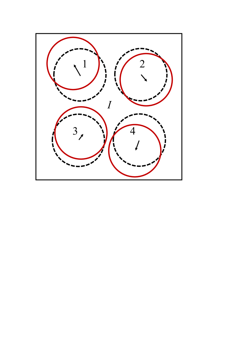
Figure 1: Vibrations of MT-spheres $n=1-4$ and the interstitial region ($I$). Dashed lines - averaged surfaces positions in the ideal structure, full (red) lines - instantaneous positions, arrows indicate the sphere diplacements $u_{n}$, $n=1-4$. As a result of sphere vibrations, the averaged quadrupole potential $\langle V_{Q}\rangle$ on the sphere surfaces is reduced, see text for details.

The electron density in the interstitial region is only weakly dependent on the amplitudes of the vibrations since the band electron on average experiences a periodic potential from the regular arrangement of the ions. On the other hand, the electron density around a nucleus being attached to it by the Coulomb interaction is expected to follow adiabatically the vibrating ion. To reconcile these apparently contradictory viewpoints we consider a model of vibrating spheres [called below muffin-tin or MT-spheres], Fig. 1, which are immersed in the crystal. We keep the values of $\rho(\vec{K})$, Eq. (11) in the interstitial region unchanged while the electron density on the vibrating sphere will be calculated taking into account the nuclear displacements. It turns out that at a finite and even zero temperature $T$ the quantities $\rho(\vec{K})$ on vibrating MT-spheres are effectively reduced (see below). In the language of the LAPW method this implies a modification of boundary conditions for the solutions inside the MT-sphere flapw , which in turn changes EFG. Therefore, our main goal is to calculate the temperature dependence of the electron density on the vibrating sphere, which later (Sec. II.4) will be used for the calculation of EFG. In the following we consider a simple case of a single atom in the primitive unit cell. (This avoids unnecessary technical complications whereas the generalization for the case of few atoms is straightforward.)

The electron density on an MT-sphere of the radius $R_{MT}$ centered at a site $n$ and displaced from the equilibrium position $\vec{X}(n)=\left\{X_{x}(n),X_{y}(n),X_{z}(n)\right\}$ by the vector $\vec{u}_{n}$ can be expanded in the multipole series

$$\rho(\vec{u}_{n},\,r=R_{MT},\theta,\phi)=\sum_{\Lambda}\rho_{\Lambda}(\vec{u}_{n})\,S_{\Lambda}(\theta,\phi),$$ (12)

where $\Lambda\equiv(l,\tau)$ stands for $A_{1g}$ irreducible representations of the crystal point group, $S_{\Lambda}(\theta,\phi)$ are corresponding symmetry adapted functions (SAFs), $l$ is the multipole orbital index and $\tau$ counts functions with the same $l$ (if there are few such functions). The polar angles $\Omega=(\theta,\phi)$ are specified by the vector $\vec{r}$ from the nuclear position ($\vec{X}+\vec{u}$). $S_{\Lambda}(\theta,\phi)$ are linear combinations of real spherical harmonics ($Y_{l}^{m,c}\sim\cos m\phi$ and $Y_{l}^{m,s}\sim\sin m\phi$) defined by the crystal site symmetry and tabulated in BC . The first function with $\Lambda=0$ ($l=0$, $\tau=1$) is the spherically symmetric (monopole) contribution, $S_{0}=Y_{l=0}^{m=0}=1/\sqrt{4\pi}$. For the hexagonal close packed structure defined by the basis vectors specified in Ref. BC the other multipole functions are: $Y_{l=2}^{m=0}$, $Y_{l=3}^{3,c}$, $Y_{l=4}^{m=0}$, $Y_{l=5}^{3,c}$, $Y_{l=6}^{m=0}$, $Y_{l=6}^{6,c}$, etc. The index $\Lambda$ runs over $(0,1)\equiv 0$, $(2,1)\equiv Q$, (3,1), (4,1), (5,1), (6,1), (6,2), etc. Thus, we have only one quadrupolar function $S_{Q}\equiv S_{l=2}=Y_{l=2}^{m=0}$, which explicitly reads as

$$S_{Q}(z)=\frac{1}{4}\sqrt{\frac{5}{\pi}}(3z^{2}-1),$$ (13)

where $z=\cos\theta$. Then the general equation (12) can be written as

$$\rho(\vec{u},\,\theta,\phi)=\frac{\rho_{0}(\vec{u})}{\sqrt{4\pi}}+\rho_{Q}(\vec{u})\,S_{Q}(\theta,\phi)$$

$$+\rho_{(3,1)}(\vec{u})\,Y_{l=3}^{3,c}(\theta,\phi)+...\;.$$ (14)

Rewriting the plane wave expansion in spherical harmonics [e.g. Eq. (34.3) of Ref. Lan ] in the complete basis set of symmetry adapted spherical harmonics [Eq. (2.4) of Ref. Nik ] one can obtain the expansion in terms of SAFs centered at the displaced nucleus of the site $n$ given by $\vec{X}(n)+\vec{u}_{n}$,

$$e^{i\vec{K}\cdot\vec{R}} = e^{i\vec{K}(\vec{X}(n)+\vec{u}_{n})}\,4\pi$$ (15)

$$\sum_{\Lambda}i^{l}j_{l}(Kr(n))S_{\Lambda}(\hat{K})\,S_{\Lambda}(\theta(n),\phi(n)).$$

Here $j_{l}$ are spherical Bessel functions and $\hat{K}$ specifies the direction of $\vec{K}$, i.e. $\hat{K}\equiv(\theta_{\vec{K}},\phi_{\vec{K}})$. From Eq. (8) then we obtain for the coefficients $\rho_{\Lambda}$, Eqs. (12), (14), at any chosen site $n$:

$$\rho_{\Lambda}(\vec{u})=4\pi i^{l}\sum_{\vec{K}}j_{l}(KR_{MT})S_{\Lambda}(\hat{K})\,\rho_{\vec{u}}(\vec{K}),$$ (16)

where $\vec{u}\equiv\vec{u}_{n}$ and

$$\rho_{\vec{u}}(\vec{K})=e^{i\vec{K}\cdot\vec{u}}\rho(\vec{K}).$$ (17)

Here we have taken into account that for vectors $\vec{K}$ and $\vec{X}(n)$ belonging to the reciprocal and direct lattice respectively, $e^{i\vec{K}\vec{X}}=1$. In the case $\vec{u}=0$ (i.e. at the equilibrium position $\vec{X}$) we get $\rho_{\vec{u}}(\vec{K})=\rho(\vec{K})$, where $\rho(\vec{K})$ is defined by Eq. (11). Averaging over the displacements at the chosen site $n$ we arrive at

$$\langle\rho_{\Lambda}\rangle=\langle\rho_{\Lambda}(\vec{u})\rangle=4\pi i^{l}\sum_{\vec{K}}j_{l}(KR_{MT})S_{\Lambda}(\hat{K})\,\langle\rho(\vec{K})\rangle,$$

(18)

where

$$\langle\rho(\vec{K})\rangle=\langle e^{i\vec{K}\cdot\vec{u}}\rangle\rho(\vec{K}).$$ (19)

Notice that Eqs. (18) and (19) are independent of $n$ because the thermal averages $\langle\rho(\vec{K})\rangle\equiv\langle\rho_{\vec{u}_{n}}(\vec{K})\rangle$ and $\langle\exp(i\vec{K}\cdot\vec{u}_{n})\rangle$ are the same for all equivalent atoms. As has been proved by Glauber Gla the thermal average on the right hand side of Eq. (19) can be transformed to

$$\langle e^{i\vec{K}\cdot\vec{u}}\rangle=e^{-W(\vec{K},T)},$$ (20)

where

$$W(\vec{K},T)=\frac{1}{2}\langle(\vec{K}\cdot u)^{2}\rangle.$$ (21)

Since the usual Debye-Waller factor is $\exp(-2W)$ Bru , the temperature function $\exp(-W)$, Eq. (20), is the square root of the Debye-Waller factor (SRDWF). Such a function has been used by Kasowski for the description of the temperature-dependent Knight shift in cadmium Kas . The function $W$ can also be written in $k-$space Bru in the familiar form

$$W(\vec{K},T)=\frac{1}{2N}\sum_{\vec{k},s}\langle(\vec{K}\cdot u_{s}(\vec{k}))^{2}\rangle,$$ (22)

where the summation runs over all vectors $\vec{k}$ in the first Brillouin zone and the phonon branches $s$, while $u_{s}(\vec{k})$ stands for the corresponding phonon amplitudes. From space symmetry considerations it follows that the function $W(\vec{K})$ is the same for a set of (non-equivalent) vectors (rays) $\vec{K}_{i}$ obtained from $\vec{K}_{1}=\vec{K}$ by the application to $\vec{K}_{1}$ all rotational or mirror symmetry elements of the crystal point group (i.e. for the vectors $\vec{K}_{i}$ belonging to the same star). In the harmonic approximation $W$ implicitly depends on the temperature through the number of thermally excited phonons $n_{\vec{K},s}$. In the Debye approximation at high temperatures ($T\gg T_{D}$) $W\sim T$.

For the calculation of EFG we need the quadrupole component ($\Lambda=(2,1)$) of the electron density and potential, Appendix A. For that purpose, with the final expressions (18), (19), (20) and (21) we obtain for the average quadrupole component $\langle\rho_{Q}\rangle$ of density on the MT-sphere in Eq. (14),

$$\langle\rho_{Q}\rangle=-4\pi\sum_{\vec{K}}j_{2}(KR_{MT})S_{Q}(\hat{K})\,e^{-W(\vec{K},T)}\,\rho(\vec{K}).\quad$$ (23)

This expression will be used later in Sec. II.4.

Since for all $\vec{K}\neq 0$ we have $W(\vec{K})>0$ even for zero temperature, the corresponding averaged Fourier components $\langle\rho(\vec{K})\rangle$ in Eqs. (18) and (19) are effectively reduced. The reduction means that as a rule the quadrupole component ($\langle\rho_{Q}\rangle$ in Eq. (14)) and also the other components with $\Lambda^{\prime}>0$ (i.e. $\langle\rho_{(3,1)}\rangle$ etc.) on the MT-sphere surface are decreased in absolute value in comparison with their static values: $|\langle\rho_{\Lambda^{\prime}}(\vec{u})\rangle|<|\rho_{\Lambda^{\prime}}(\vec{u}=0)|$. As will be discussed below in Sec. II.4 the effective decrease of $\langle\rho_{Q}\rangle$ occurs also in the interior of the MT-sphere, $r\leq R_{MT}$, and finally leads to a reduction of EFG. In some rare cases as a result of the interplay between terms of opposite signs in Eq. (23) an increase of $\langle\rho_{Q}\rangle$ can occur. Such a situation is discussed in detail below in Sec. III.3.

The reduction or increase of $\langle\rho_{Q}\rangle$ however does not affect the total charge of the sphere because the integral over the polar angles for SAFs $S_{Q}$, $Y_{3}^{3,c}$ and the others with $l\neq 0$ are zero. The total charge of the sphere is due to the monopole term ($l=0$), which is closely related to the $\vec{K}=0$ term in the Fourier expansion of density, Eq. (8). Notice that the $\rho(K=0)$ component is independent of $T$, Eq. (19), keeping the total charge inside the sphere approximately constant. A very small decrease of the average value of $\langle\rho_{0}\rangle$ in Eq. (14) (implying a small increase of the charge in the interstitial region) can be accounted for by a small increase of the $\rho(K=0)$ component of the Fourier expansion (8). In our calculations the effect is found small and has been neglected.

In the following we shall apply our approach to the case of the hexagonal close packed structure, although in principle the consideration is general and can be used for other non-cubic lattices.

II.3 EFG and quadrupole ($L=2$) expansion of the electron potential around the nucleus

In this section we demonstrate that the reduction (or increase) of $\langle\rho_{Q}\rangle$ inside the MT-sphere results in a corresponding change of the quadrupole component of the potential and the electric field gradient.

Similarly to the density expansion, Eq. (12), the electron self-consistent-field Coulomb potential of the general form around a nucleus, employed for example in the full potential linearized augmented plane wave method (FLAPW) flapw ; wien2k , also can be expanded in multipolar series,

$$V(r,\theta,\phi)=\sum_{\Lambda}V_{\Lambda}(r)\,S_{\Lambda}(\theta,\phi).$$ (24)

Notice that the coefficients $V_{\Lambda}(r)$ for the potential and $\rho_{\Lambda}(r)$ for electron density, Eq. (12), can be obtained from ab initio electron band structure calculations. In Figs. 2 and 3 we reproduce such dependencies for the quadrupole component, $l=2$.

From a scrupulous analysis of the multipolar components of the potential (see Appendix A and Ref. Nik ) it follows that in the neighborhood of the nucleus (when $r\ll 1$) the radial dependence of the function $V_{l,\tau}$ reads as

$$V_{\Lambda}(r)=v_{\Lambda}\,r^{l},$$ (25)

where $v_{\Lambda}$ is a constant. This in particular implies that for quadrupolar component [$\Lambda=(2,1)$] we have $V_{Q}\equiv V_{(2,1)}(r)=v_{Q}\,r^{2}$, for the component $\Lambda=(4,1)$ $V_{(4,1)}(r)=v_{(4,1)}\,r^{4}$, etc. This dependence of $V_{Q}(r)$ is illustrated in Fig. 3. It is worth noting that the quadrupolar electron density component also follows the same law close to the nucleus, i.e. $\rho_{Q}(r)\propto r^{2}$, Fig. 3.

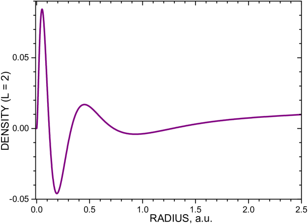
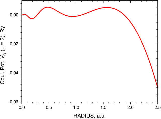
Figure 2: DFT calculation of the quadrupole ($l=2$) component $\rho_{Q}(r)$ of electron density (top panel) and the corresponding Coulomb potential $V_{Q}(r)$ (bottom panel) inside the MT-sphere of the hcp structure of Zn ($a=2.659$ Å, $c=4.851$ Å, $R_{MT}=1.33$ Å or 2.51 a.u.).

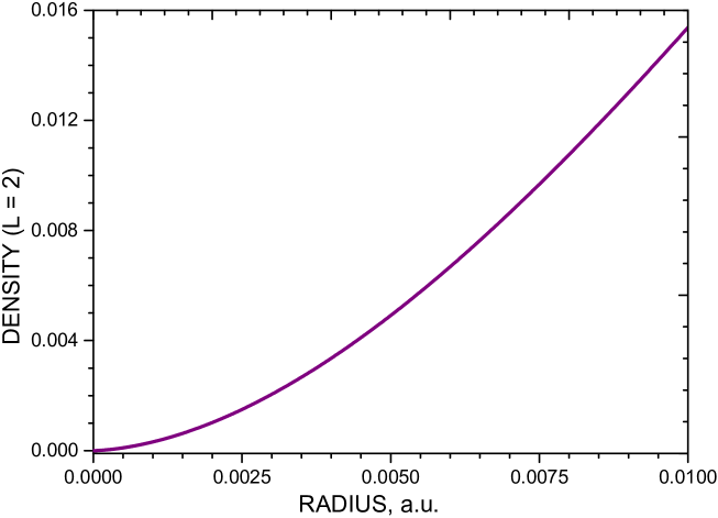
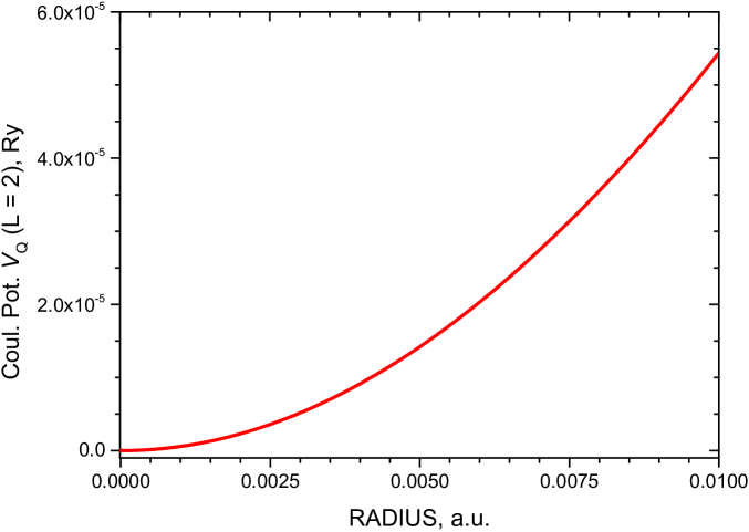
Figure 3: DFT calculation of the quadrupole ($l=2$) component $\rho_{Q}(r)$ of electron density (top panel) and the corresponding Coulomb potential $V_{Q}(r)$ (bottom panel) of the hcp structure of Zn in the vicinity of nucleus. (Fig. 3 zoomed at $r=0$.) Both the density and potential are proportional to $r^{2}$. For comparison, the Zn nuclear radius is $9.1\cdot 10^{-5}$ a.u.

Taking Eq. (25) into account, we obtain for the electric field gradient,

$$V_{zz}=\frac{\partial^{2}V_{Q}}{\partial z^{2}}=\sqrt{\frac{5}{\pi}}\,v_{Q}.$$ (26)

Details are given in Appendix A. Notice that Eq. (26) gives a temperature independent EFG.

The quadrupole potential on the MT-sphere, $V_{Q}^{S}$ consists of two contributions,

$$V_{Q}^{S}=V_{Q}^{S,\,out}+V_{Q}^{S,\,in}.$$ (27)

Here, $V_{Q}^{S,\,out}$ and $V_{Q}^{S,\,in}$ are the potentials due to all charges outside the MT-sphere and inside it, respectively. Correspondingly, for the quadrupole potential $V_{Q}$ at any point $\vec{r}=(r,\,\theta,\phi)$ inside the MT-sphere we have

$$V_{Q}(\vec{r})=V_{Q}^{out}(\vec{r})+V_{Q}^{in}(\vec{r}),$$ (28a)

where

$$V_{Q}^{out}(r,\theta,\phi)=V_{Q}^{S,\,out}\frac{r^{2}}{R_{MT}^{2}}\,S_{Q}(\theta,\phi),$$ (28b)

(for hcp lattices $$S_{Q}=Y_{2}^{0}$$) and

$$V_{Q}^{in}(r,\theta,\phi)=\frac{4\pi}{5}\left(\frac{q_{Q}(r)}{r^{3}}+r^{2}q^{\prime}_{Q}(r)\right)S_{Q}(\theta,\phi).$$ (28c)

Here

$$q_{Q}(r)=\int_{0}^{r}\rho_{Q}(r^{\prime})\,{r^{\prime}}^{3}dr^{\prime},$$ (29a)

$$q^{\prime}_{Q}(r)=\int_{r}^{R_{MT}}\frac{\rho_{Q}(r^{\prime})}{r^{\prime}}dr^{\prime},$$ (29b)

Since $q^{\prime}_{Q}(R_{MT})=0$, we find $V_{Q}^{S,\,in}=4\pi q(R_{MT})/R_{MT}^{3}$. Notice that $V_{Q}^{out}$ is explicitly proportional to $r^{2}$, Eq. (28b). It can be shown Nik that the same holds for $V_{Q}^{in}$ at $r\ll 1$. From Eqs. (25), (26) we then arrive at

$$V_{zz}=\sqrt{\frac{5}{\pi}}\left(v_{Q}^{out}+v_{Q}^{in}\right).$$ (30)

Here $v_{Q}^{out}$ and $v_{Q}^{in}$ are obtained from $V_{Q}^{out}/r^{2}$ and $V_{Q}^{in}/r^{2}$ when $r\rightarrow 0$. As a result of the reduction of $\langle\rho_{Q}(r)\rangle$ with temperature, $\langle v_{Q}^{out}\rangle$ and $\langle v_{Q}^{in}\rangle$ also become reduced, and $\langle V_{zz}\rangle$ decreases with temperature.

II.4 Temperature dependence of EFG

As shown in Sec. II.2 the average quadrupole density component $\langle\rho_{Q}(R_{MT})\rangle$ on the vibrating MT-sphere as a rule is reduced, Eq. (23). However, to calculate exactly the effect of the reduction on EFG, we have to know $\langle\rho_{Q}(r)\rangle$ at all values $r\leq R_{MT}$, see Sec. II.3. In a straightforward approach we should perform a calculation for $\langle\rho_{Q}(r)\rangle$ inside the MT-sphere considering the new value of $\langle\rho_{Q}(R_{MT})\rangle$, Eq. (23), as an input boundary condition. In practice, by changing $R_{MT}$ in a range close to the maximal (contact) radius $R_{max}$, we have found that the reduction of the quadrupolar density component, $\rho_{Q}(r,T)/\rho_{Q}(r,\,T=0)$, is approximately constant. In Zn for example the change of $R_{MT}$ from the $R_{max}$ value of 2.517 a.u. to 2.30 a.u. at 300 K results in a change of the ratio from 0.945 to 0.926 (2%). We then in a first approximation assume that for all $r\leq R_{MT}$

$$\frac{\rho_{Q}(r,T)}{\rho_{Q}(r,\,T=0)}=\frac{\rho_{Q}(R_{MT},T)}{\rho_{Q}(R_{MT},\,T=0)}=R^{in}(T).$$ (31)

Accoring to Eqs. (29a) and (29b), the reduced quadrupolar density component $\langle\rho_{Q}(r,T)\rangle$ for all $r\leq R_{MT}$ changes the quadrupole charges as $q_{Q}(r,T)=R^{in}(T)\,q_{Q}(r)$ and $q^{\prime}_{Q}(r,T)=R^{in}(T)\,q^{\prime}_{Q}(r)$. This in turn leads to the reduction of $V_{Q}^{in}(T)=R^{in}(T)\,V_{Q}^{in}$, Eq. (28c), and $v_{(2,0)}^{in}(T)=R^{in}(T)\,v_{(2,0)}^{in}$. We then for the temperature evolution of EFG have

$$V_{zz}(T)=\sqrt{\frac{5}{\pi}}\left(R^{out}(T)\,v_{(2,0)}^{out}+R^{in}(T)\,v_{(2,0)}^{in}\right)$$

(32)

[compare with Eq. (30)]. Here the factor $R^{out}(T)$ accounts for the change of the potential due to all charges outside the MT-sphere, while $v_{(2,0)}^{out}$ and $v_{(2,0)}^{in}$ are temperature independent (calculated with an ab initio electron band structure method). In practice, $v_{(2,0)}^{out}$ is found to be small (1-3 %) compared to $v_{(2,0)}^{in}$. Since, in addition the difference between $R^{out}$ and $R^{in}$ is not essential, in the following for simplicity we take $R^{out}\approx R^{in}$. Then the temperature dependence of EFG is completely due to the change of $\rho_{Q}$ inside the MT-sphere and

$$V_{zz}(T)\approx R^{in}(T)V_{zz}.$$ (33)

Eqs. (33) and (31) imply that we consider the change of the quadrupole interaction as a perturbation causing a linear effect inside the MT-sphere.

II.5 Mean-square displacements

The SRDW factor, Eqs. (20) and (21) depends crucially on the mean square displacements $\langle u_{x}^{2}\rangle$, $\langle u_{y}^{2}\rangle$ and $\langle u_{z}^{2}\rangle$, which are functions of temperature. For the hcp lattice $\langle u_{x}^{2}\rangle=\langle u_{y}^{2}\rangle$, and for calculations of SRDWF we need to know only two functions: $U_{11}(T)=\langle u_{x}^{2}\rangle$ and $U_{33}(T)=\langle u_{z}^{2}\rangle$ (for hcp lattice $U_{33}>U_{11}$),

$$W(\vec{K},T)=\frac{1}{2}\left((K_{x}^{2}+K_{y}^{2})\,U_{11}(T)+K_{z}^{2}\,U_{33}(T)\right).$$ (34)

The functions $U_{11}(T)$ and $U_{33}(T)$ can be calculated within the harmonic approximation or extracted experimentally as illustrated in Fig. 4 for the hcp lattice of Zn.

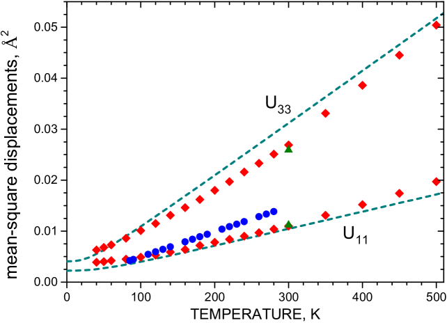
Figure 4: Temperature evolution of $U_{11}=\langle u_{x}^{2}\rangle$ and $U_{33}=\langle u_{z}^{2}\rangle$ for hcp Zn found by various methods. Dark cyan dash lines stand for calculations in the harmonic approximation (DFPT of QE QE1 ; QE2 ), red diamonds are experimental data from the single crystal structural refinement of Zn at different $T$ Nus , olive triangles are experimental data at $T=300$ K Ske , blue circles are obtained from experimentally determined phonon density of states Pen .

In Fig. 5 we plot individual SRDW factors, $\exp(-W(\vec{K},T))$, for the hcp structure of Zn, which are responsible for the temperature reduction of the quadrupole density and potential, Sec. II.2. With the increase of $T$ the SRDW factors get shifted to lower values. A finite width of SRDWF for reciprocal vectors with close values of $|\vec{K}|$ is due to different orientations of $\vec{K}$ in respect to the ellipsoid of mean-square displacements. The width becomes larger with the increase of asymmetry between $U_{11}$ and $U_{33}$.

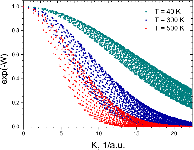
Figure 5: Square root of the Debye-Waller factors (SRDWF), $\exp(-W(\vec{K},\,T))$, as functions of the modulus of reciprocal vectors $K=|\vec{K}|$ of hcp Zn for various temperatures. Dark cyan circles are data for $T=40$ K, blue squares - $T=300$ K and red triangles - $T=500$ K. Calculations are based on experimental data for the mean-square displacements $U_{11}(T)$ and $U_{33}(T)$, Ref. Nus .

III Application to zinc and cadmium

In this section we apply the method described earlier to calculations of the temperature dependence of the electric field gradient of solid zinc and cadmium crystallized in the hexagonal close packed lattice.

For that we need data on the Fourier expansion of the electron density in the interstitial region, quadrupole components of electron density and potential obtained from the electron band structure calculations. Electron density functional calculations have been performed with the Moscow-FLAPW code lapw . The code explicitly takes into account the nuclear size and the change of the potential and the wave function inside the nuclear region to obtain the electric field gradient accurately. In addition, the number of radial points inside the MT-region has been increased to 3000 (for some runs 3500). The typical LAPW basis set cut-off parameter was $R_{MT}K_{max}$ = 9 (the number of basis functions 221), the number of $k$ points was 704 (1331), the maximal value of the LAPW plane wave expansion $l_{max}=10$. We have used the tetrahedron method for the linear interpolation of energy between $k$ points tet . For calculation of the exchange-correlation potential and the exchange-correlation energy contribution we have used the Perdew-Burke-Ernzerhof (PBE) variant PBE of the generalized-gradient approximation (GGA) within the density functional theory (DFT) at experimental lattice constants at room temperature [$a=2.663$ Å, $c=4.944$ Å, $R_{MT}=1.196$ Å (Zn) and $a=2.996$ Å, $c=5.674$ Å, $R_{MT}=1.429$ Å (Cd).]

Also, the temperature evolution of the tensor of mean-square displacements, $U_{11}(T)$ and $U_{33}(T)$, is required for the calculation of the square root of the Debye-Waller factor, $\exp(-W(\vec{K},T))$, for vectors $\vec{K}$ of the reciprocal lattice, Eqs. (34) and (20). The temperature evolution of the tensor of mean-square displacements can be obtained by three different ways: (1) from a direct experimental parametrization of the displacements $\langle u_{x}^{2}(T)\rangle$ and $\langle u_{z}^{2}(T)\rangle$ as given in Ref. Nus for Zn; (2) from calculations of the phonon frequencies and eigenvectors (for example, within the DF perturbation treatment of lattice dynamics with Quantum Espresso QE1 ; QE2 ); (3) from effective Debye temperature $T_{D}(T)$ which appear as a result of experimental parametrization Kri ; Pen . The strict harmonic approximation is adopted only in (2), while in (1) and (3) an anharmonic effects such as thermal expansion of solids and phonon softening are effectively taken into account. Experimentally, the values of $\langle u_{x}^{2}(T)\rangle$ and $\langle u_{z}^{2}(T)\rangle$ (or directly related to them temperature factors $B_{x}(T)$ and $B_{z}(T)$ Pen ) are found from the temperature evolution of the x-ray diffraction spectra.

For the phonon part (2) of calculations the first-principles pseudopotential method as implemented in the Quantum Espresso (QE) package QE1 ; QE2 with the PBE exchange-correlation functional PBE has been employed. The projected-augmented-wave (PAW) type scalar-relativistic pseudopotentials have been taken from the standard solid-state pseudopotential (SSSP) library sssp1 ; sssp2 . The integration over the Brillouin zone (BZ) for the electron density of states has been performed on a $24\times 24\times 12$ grid of $k$-points, the plane-wave kinetic cut-off energy was 70 Ry. The lattice-dynamical calculations have been carried out within the density-functional perturbation theory (DFPT). Phonon dispersions have been computed using the interatomic force constants based on a $6\times 6\times 4$ $k$-point grid, with a $48\times 48\times 24$ grid used to obtain the phonon densities of states and $U_{11}(T)$ and $U_{33}(T)$.

III.1 Zinc

Mean-square displacements for hcp structure of zinc are shown in Fig. 4. First, we notice that in the DFPT-QE harmonic approximation in the region of $T$ from 60 K to 500 K, $U_{11}(T)$ and $U_{33}(T)$ are practically linear in $T$. Such behaviour is also expected in the Debye model for $T>T_{D}$. Experimentally, however we observe that $U_{11}(T)$ and $U_{33}(T)$ deviate from the linear law. As shown in Ref. Nus $U_{11}(T)$ and $U_{33}(T)$ are approximated by quadratic functions of $T$ for all data in the range from 40 K to 500 K. In addition, in the harmonic approximation values of $U_{33}$ are slightly overestimated, Fig. 4, which results in a considerable suppression of the SRDF factors and the calculated temperature dependence of EFGs, Fig. 6.

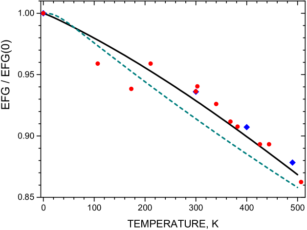
Figure 6: Temperature dependence of electric field gradient in Zn, $V_{zz}(T)/V_{zz}(T=0)$. Calculations – solid black line – are based on experimental data for the mean-square displacements $U_{11}(T)$ and $U_{33}(T)$, Ref. Nus . DFPT-QE calculations QE1 ; QE2 – dark cyan dash line – have been made in the harmonic approximation. Red circles Chris and blue diamonds Bertschat stand for experimental data on EFG ratios.

On the other hand, our calculations of the temperature evolution of EFG using experimental data for $U_{11}(T)$ and $U_{33}(T)$ demonstrate a good correspondence with the measured values of $V_{zz}$, Fig. 6. We have also found that the $T$ dependence of $V_{zz}$ is extremely sensitive to the ratio ${\cal R}=U_{33}/U_{11}$. To demonstrate it we have computed the evolution of $V_{zz}$ with $T$ with reduced values of ${\cal R}$, Fig. 7(upper panel). It turns out that if ${\cal R}=1$ [i.e. $U_{33}(T)=U_{11}(T)$] there is virtually no temperature decrease of EFG, although we have kept the average value of mean-square displacements

$$U_{av}=(2U_{11}+U_{33})/3$$ (35)

growing with $T$ according to experimental data Nus . It is worth mentioning that the experimental behavior of $U_{33}/U_{11}$ in Zn is highly nonlinear in contrast to the simple linear increase of the lattice constant ratio $c/a$ Nus . On the other hand, in the harmonic approximation $U_{33}/U_{11}$ should be almost independent of $T$, at least for $T>T_{D}\sim 200$ K Ske . Therefore, in the $T$ dependence of $U_{33}/U_{11}$ and consequently of EFG there is a substantial anharmonic contribution.

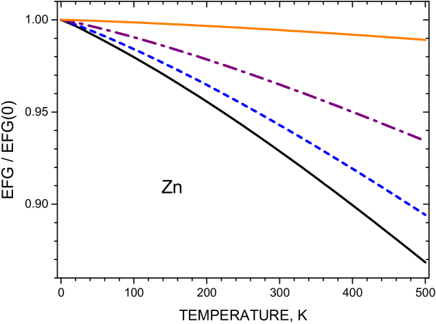
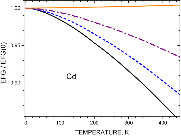
Figure 7: Evolution of the $T$ dependence of $V_{zz}$ with a reduction of the mean square displacement ratio ${\cal R}=U_{33}/U_{11}$ while keeping the averaged value of the displacements $U_{av}$, Eq. (35), unchanged. Black solid line corresponds to the initial value of ${\cal R}_{0}=U_{33}/U_{11}$, the others - to reduced ${\cal R}$. Blue dashed line: ${\cal R}=1+(2/3)\cdot({\cal R}_{0}-1)$, purpled dot-dash line: ${\cal R}=1+(1/3)\cdot({\cal R}_{0}-1)$, orange solid line: ${\cal R}=1$ or $U_{33}=U_{11}$. Top panel - zinc, bottom panel - cadmium. A weak increase of $V_{zz}$ with $T$ (orange solid line in Cd) is discussed in Sec. III.3.

In particular, the anharmonic effect is responsible for the negative curvature of $V_{zz}$ in contrast to the approximate linear dependence of the harmonic model, Fig. 6.

Notice, that even at zero temperature the value of EFG is slightly reduced because of the zero point vibrations. The calculated reduction is 0.6% with the mean square displacements from Ref. Nus and 1% according to DFPT-QE. The refined calculated absolute value of EFG is $V_{zz}=3.51\times 10^{21}$ V/m², the corrected for the zero point vibrations Nus – $V_{zz}=3.49\times 10^{21}$ V/m². It corresponds to the quadrupole frequency 10.53 MHz for $Q($Zn$)=0.125$ b Haa and 12.64 MHz for $Q($Zn$)=0.15$ b, which compares well with the experimental value of 12.34 MHz at 4.2 K Pot .

III.2 Cadmium

Results for cadmium are given in Figs. 8 and 9.

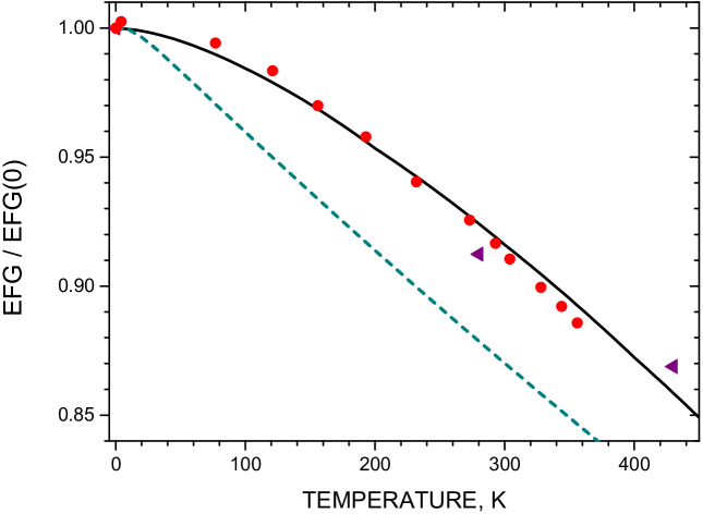
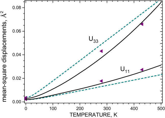
Figure 8: Temperature evolution of $V_{zz}$ in Cd (upper panel) determined by the mean-square displacements $U_{11}$ and $U_{33}$ (lower panel). Red circles stand for experimental measurements Chris , black line – for a present model calculation taking into account softening of the lattice and an increase of $U_{33}/U_{11}$ with $T$ (see text for details), dark cyan dash line – DFPT-QE calculations QE1 ; QE2 . Purple triangles are our calculations with mean-square displacements of Table II of Ref. Toru (the Phonon code phonon within the harmonic approximation).

As for the zinc calculation we observe that the mean-square displacements $U_{33}$ are overestimated by the DFPT-QE calculations. In addition, DFPT-QE values of $U_{33}$ are underestimated in comparison with other models. Both effects lead to a fast decrease of $V_{zz}$ with temperature, although in the region of 260-360 K the DFPT-QE harmonic treatment gives the correct slope for the $V_{zz}$ decrease. As for zinc our calculations of the temperature evolution of $V_{zz}$ in Cd have turned out to be very sensitive to values of mean square displacements $U_{11}$ and $U_{33}$, especially to ${\cal R}=U_{33}/U_{11}$. It is worth noting that with the mean-square values obtained by Torumba et al Toru with the Phonon program phonon , we have obtained reduced EFGs which compares well with the experimental results of Ref. Chris at 280 K and 430 K, Fig. 8. However, our calculations also show that these values of $U_{11}$ and $U_{33}$ somewhat underestimate the reduction of $V_{zz}$ at 430 K and especially at 570 K (not shown in Fig. 8). We believe that this is related to the softening of the Cd lattice Ske and increase of the ratio of ${\cal R}$ with temperature which lays beyond the harmonic approximation. In fact, as we know from experimentally deduced values of $U_{11}$ and $U_{33}$ Nus both effects are clearly present in the case of Zn lattice, Fig. 4. Since at the moment there are no experimental data for the mean-square displacements of cadmium, we have performed a number of model calculations, Fig. 9.

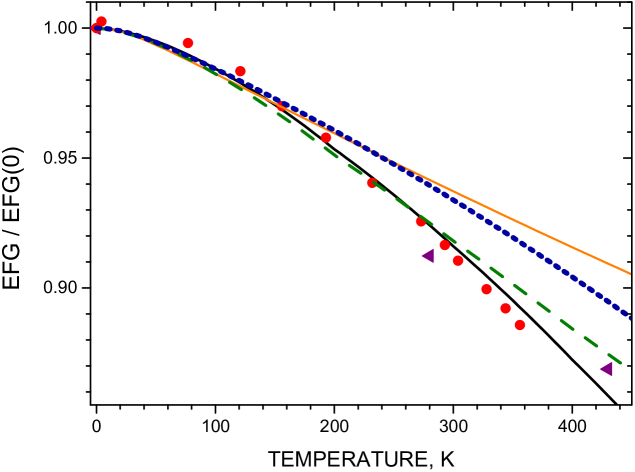
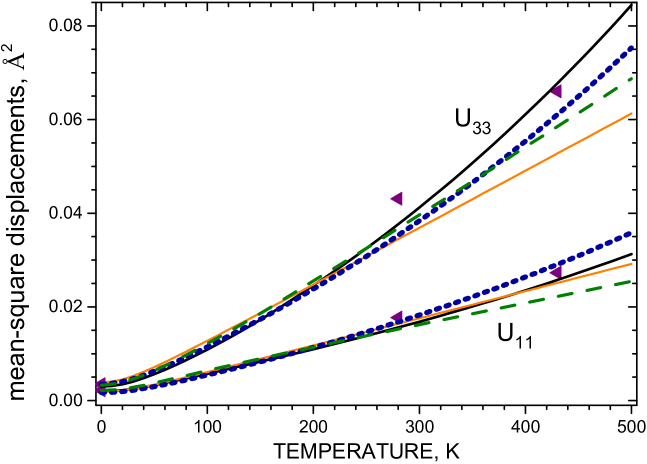
Figure 9: Model mean-square displacements $U_{11}$ and $U_{33}$ in Cd (lower panel) and corresponding temperature dependencies of $V_{zz}$ (upper panel). Red circles stand for experimental measurements Chris , black line – for a model calculation taking into account the softening of the lattice and the increase of $U_{33}/U_{11}$ with $T$. Yellow solid line – calculations without softening and the $U_{33}/U_{11}$ ratio fixed; blue dotted line – with the softening and the $U_{33}/U_{11}$ ratio fixed; green dashed line – without softening, the $U_{33}/U_{11}$ ratio increased, see text for details. Purple triangles are our calculations with mean-square displacements of Table II of Ref. Toru .

The averaged mean square displacement $U_{av}=(2U_{11}+U_{33})/3$ has been calculated within the Debye lattice model with a temperature dependent Debye temperature $T_{D}$. The lattice softening has been modelled by a linear decrease of $T_{D}$, from 140 K (at $T=0$ K) to 115 K (at $T=500$ K), with the averaged value of $T_{D}^{av}=127.5$ K. [These value is very close to $T_{D}=$131$\pm$7 K given in Ref. Kris for Cd.] In addition, we consider an anharmonic effect modelled by a linear change of ${\cal R}$ from 1.5 (at $T=0$ K) to 2.7 (at $T=500$ K) with the averaged value of ${\cal R}=2.1$. Correspondingly, we have performed four model calculations shown in Fig. 9: (1) with the lattice softening and the temperature increase of ${\cal R}$ (black curve in Fig. 9), (2) without softening and with ${\cal R}$ fixed (yellow curve), (3) with the softening and ${\cal R}$ fixed (blue dotted line), (4) without softening and with ${\cal R}$ increased (dashed green line). The results clearly demonstrate that the best fit is achieved with the lattice softening and the temperature increase of ${\cal R}$ with $T$, while other models deviate from the experimental data at elevated temperatures. Although these arguments can not be considered as a solid proof, the important finding is that both unharmonic effects improve the comparison with the experiment.

The calculated absolute value of EFG is $V_{zz}=7.82\times 10^{21}$ V/m². The zero point vibration contribution to $V_{zz}$ amounts to 0.8% according to DFPT-QE and 0.4% in the model (1). The corrected for the zero point vibrations value [model (1)] is $V_{zz}=7.79\times 10^{21}$ V/m², which corresponds to $\nu_{Q}=120.7$ MHz (adopting $Q($Cd$)=0.641$ b Haa ) or $\nu_{Q}=143.1$ MHz (with $Q($Cd$)=0.76$ b Err ). Extrapolated to $T=0$ quadrupole frequency in metallic cadmium is 136.9 MHz Chris .

III.3 Mechanism of increase of EFG with $T$

The most important factor in the $T$ dependence of EFG is ${\cal R}=U_{33}/U_{11}$. As discussed in Sec. III.1, B and shown in Fig. 7, the ratio ${\cal R}$ has a pronounced influence on the shape of the $V_{zz}(T)$ curve. A reduction of ${\cal R}$ in cadmium also has an immediate and sizeable effect on $V_{zz}(T)$, Fig. 7. Interestingly, for ${\cal R}=1$ [$U_{11}=U_{33}$] we observe in cadmium a rare effect of a weak increase of $V_{zz}$ with $T$ (orange plot in Fig. 7). At first sight, this seems incompatible with the apparent reduction of $\langle\rho_{Q}\rangle$, Eq. (23), caused by $\exp(-W)$. Notice however, that in the sum on the right hand side of Eq. (23) individual contributions proportional to $j_{2}(KR_{MT})S_{Q}(\hat{K})\langle\rho(\vec{K})\rangle$ are of different signs. Two such principal groups of terms can be schematically written as

$$V_{zz}(T)\propto\langle\rho_{Q}\rangle=\sum[c_{1}\,{\cal W}_{1}\,\rho(\vec{K}_{1})-c_{2}\,{\cal W}_{2}\,\rho(\vec{K}_{2})].$$ (36)

Here the $T$ dependent SRDWFs are incorporated in the weight factors ${\cal W}_{i}=\exp(-W(\vec{K}_{i},\,T))$ and $c_{i},\,\rho(\vec{K}_{i})>0$ ($i=1,2$). Both ${\cal W}_{1}$ and ${\cal W}_{2}$ reduce with $T$, but if ${\cal W}(\vec{K}_{2},\,T)$ drop fast enough in comparison with ${\cal W}(\vec{K}_{1},\,T)$, one can have a resulting increase of the expression in the square brackets of (36) and of the whole sum.

Our detailed numerical analysis for the situation is illustrated further in Fig. 10. One can see that at $T=300$ K positive contributions to the gradient (red circles) although appreciably suppressed by negative contributions (blue diamonds), finally prevail, which leads to a small positive net contribution to EFG (the $n=120$ value of the dashed purpled curve). At $n\geq 120$ the positive sum value is virtually unchanged.

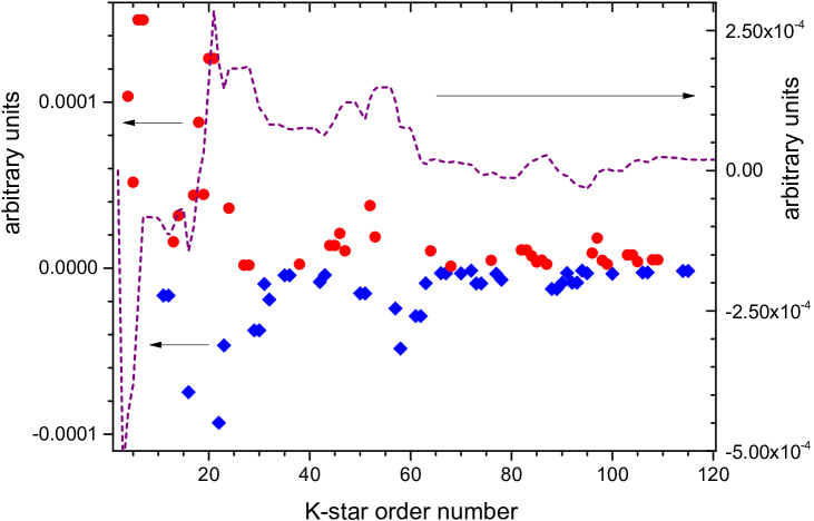
Figure 10: Individual $K-$star contributions to electric field gradient at $T=300$ K [each term $\propto j_{2}(KR_{MT})S_{Q}(\hat{K})(\langle\rho(\vec{K})\rangle_{T=300}-\langle\rho(\vec{K})\rangle_{T=0})$, Eq. (23)]. Blue diamonds - negative contributions, red circles - positive contributions, dashed purpled curve - sum of all contributions up to the chosen $K-$star. The final value of the sum (at $n\geq 120$) is positive, which leads to an increase of $V_{zz}$ at 300 K.

IV Conclusions

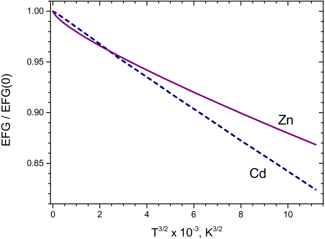
Figure 11: Plots of the $T$ dependence of electric field gradient, $V_{zz}(T)/V_{zz}(T=0)$ for Zn and Cd as functions of $T^{3/2}$.

We have presented a new method which can describe the temperature evolution of electric field gradient $V_{zz}$ in metals. The consideration is based on the fact that the average value of the quadrupole component $\langle\rho_{Q}\rangle$ of electron density on a sphere vibrating with the nucleus, Eq. (23), is changed with $T$. The effective reduction of each Fourier component $\rho(\vec{K})$ of density, Eqs. (19), (20) and (21), is given by the multiplier $\exp(-W(\vec{K},T))$ which is the square root of the usual Debye-Waller factor. The method relies on DFT calculations of electron properties and the dependence of mean-square displacements $U_{11}$ and $U_{33}$ on temperature. We have found that the form and pace of the temperature change of $V_{zz}$ is very sensitive to the mean-square displacements $U_{11}(T)$, $U_{33}(T)$, and in particular to their ratio $U_{33}(T)/U_{11}(T)$. The model is capable of reproducing both a decrease or increase of EFG with temperature. The unusual mechanism of increase of $V_{zz}$ with $T$ is discussed in Sec. III.3.

We have applied our method to hexagonal close packed structures of pristine zinc and cadmium. In the case of zinc where the mean-square displacements $U_{11}(T)$ and $U_{33}(T)$ are known experimentally from single crystal x-ray diffraction Nus , we obtain a very good description of the temperature change of EFG, Fig. 6. In the case of cadmium the behaviour of $V_{zz}(T)$, Fig. 8, can be reproduced by assuming two anharmonic effects: the lattice softening (modelled by a decrease of the Debye temperature $T_{D}$ with $T$), and an increase of the ratio $U_{33}/U_{11}$ with $T$. It is worth noting that both anharmonic effects are also present in zinc Ske ; Nus .

In addition, we have performed calculations of the mean-square displacements in Zn and Cd in the harmonic approximation by using the DF perturbation treatment of the QE package QE1 ; QE2 . For both metals an approximately linear dependence in $T$ for $U_{11}(T)$ and $U_{33}(T)$ (at $T>40$ K) and consequently for the calculated $V_{zz}$ curves has been found. In the case of cadmium, the decrease of EFG has been exaggerated which can be accounted for by an uncertainty related to its core pseudopotential sssp1 ; sssp2 . Using the mean-square displacements calculated at $T=280$ and 430 K by Torumba et al. Toru with the package Phonon phonon , we have obtained reduced values of EFG which lie not far from the experimental data.

In our studies we have not found an intrinsic mechanism for the $T^{3/2}$ dependence of EFG, Eq. (2). Nevertheless, the $T^{3/2}$ plots, Fig. 11, indicate that an approximate $T^{3/2}$ law for Zn and Cd holds. For Cd the dependence is almost perfect, for Zn it deviates from $T^{3/2}$ at low temperatures which can be partially explained by the fact that the experimental data for mean-square displacements Nus are available only for $T>40$ K. In any case, even experimental data for EFG of Zn and Cd deviate from the $T^{3/2}$ law at low temperatures Verma . We therefore conclude that the mechanism of the temperature dependence of $V_{zz}$ in Zn and Cd is complex, with a substantial contribution from anharmonic effects. An approximate correspondence with the $T^{3/2}$ dependence is probably due to the $T$ behavior of SRDW factors, $\exp(-W)$ Jen .

Finally, we mention that even at zero temperature the measured EFGs are smaller than $V_{zz}$ calculated by ab initio methods. The zero temperature reduction however is small: 0.6% in Zn and 0.4% in Cd.

Appendix A Quadrupolar potential and the tensor of EFG

The asymptotic behavior of the potential close to the nucleus, Eq. (25), can be understood from the two center expansion of the Coulomb potential in double multipolar series,

$$\frac{1}{|\vec{R}(\vec{n})-\vec{R}^{\prime}(\vec{n}^{\prime})|}$$

$$=\sum_{\Lambda\Lambda^{\prime}}v_{\Lambda\Lambda^{\prime}}(\vec{n},\vec{n}^{\prime};\,r,r^{\prime})\,S_{\Lambda}(\hat{r}(\vec{n}))\,S_{\Lambda^{\prime}}(\hat{r}^{\prime}(\vec{n}^{\prime})),$$ (37)

where the interaction strength $v_{\Lambda\Lambda^{\prime}}$ is given by Hei

$$v_{\Lambda\Lambda^{\prime}}(\vec{n},\vec{n}^{\prime};\,r,r^{\prime})\sim\frac{(r)^{l}(r^{\prime})^{l^{\prime}}}{|\vec{X}(\vec{n})-\vec{X}(\vec{n}^{\prime})|^{l+l^{\prime}+1}},$$ (38)

Here $\vec{R}(\vec{n})=\vec{X}(\vec{n})+\vec{r}(\vec{n})$ is the radius vector close to the crystal site $\vec{n}$. For $r\ll 1$ we arrive at Eq. (25) which holds both for the contributions from the electron density around the site $\vec{n}$ and the contributions from the densities on the other sites $\vec{n^{\prime}}\neq\vec{n}$.

As follows from Eqs. (24), (25), the quadrupolar component of the potential for the hexagonal lattice can be written as

$$V_{Q}(r,\theta,\phi) = v_{Q}\,r^{2}\,Y_{l=2}^{m=0}(\theta,\phi)$$ (39)

$$= v_{Q}\,\frac{1}{4}\sqrt{\frac{5}{\pi}}(3z^{2}-r^{2}).$$

[We recall that here $v_{Q}=v_{(2,1)}$ is a constant.] From this relation we obtain that the tensor of EFG is diagonal in the Cartesian system of axis and

$$V_{zz}=\frac{\partial^{2}V_{Q}}{\partial z^{2}}=\sqrt{\frac{5}{\pi}}\,v_{Q},$$ (40)

$$V_{xx}=\frac{\partial^{2}V_{Q}}{\partial x^{2}}=\frac{\partial^{2}V_{Q}}{\partial y^{2}}=-\frac{1}{2}\sqrt{\frac{5}{\pi}}\,v_{Q}.$$ (41)

References

- (1) E. N. Kaufmann and R. J. Vianden, Rev. Mod. Phys. 51, 161 (1979).
- (2) T.P. Das and P.C. Schmidt, Z. Naturforsch. 41a, 47 (1986).
- (3) H. Haas, Hyperfine Interact. 129, 493 (2000).
- (4) Handbook of Applied Solid State Spectroscopy, Ed. D.R. Vij, Springer-Verlag US (2006).
- (5) T. Wichert, E. Recknagel, Perturbed Angular Correlation. In: Gonser U. (eds) Microscopic Methods in Metals. Topics in Current Physics, vol 40. Springer, Berlin, Heidelberg (1986).
- (6) J. Schell, P. Schaaf, and D. C. Lupascu, AIP Advances 7, 105017 (2017).
- (7) L. Hemmingsen, K. N. Sas, and E. Danielsen, Chem. Rev. 104, 4027 (2004).
- (8) R. Dogra, A. P. Byrne, and M. C. Ridgway, Journal of Elec. Mater. 38, 623 (2009).
- (9) A. V. Tsvyashchenko, D. A. Salamatin, V. A. Sidorov, A. E. Petrova, L. N. Fomicheva, S. E. Kichanov, A. V. Salamatin, A. Velichkov, D. R. Kozlenko, A. V. Nikolaev, G. K. Ryasny, O. L. Makarova, D. Menzel, and M. Budzynski. Phys. Rev. B 92, 104426 (2015).
- (10) P. Blaha, K. Schwarz, and P. Herzig, Phys. Rev. Lett. 54, 1192 (1985).
- (11) P. Blaha, K. Schwarz, and P. H. Dederichs, Phys. Rev. B 37, 2792 (1988).
- (12) H. M. Petrilli, P. E. Blöchl, P. Blaha, and K. Schwarz, Phys. Rev. B 57, 14690 (1998).
- (13) L. Errico, K. Lejaeghere, J. Runco, S. N. Mishra, M. Renteria, S. Cottenier, J. Phys. Chem. C 120, 23111 (2016).
- (14) H. Haas, S. P. A. Sauer, L. Hemmingsen, V. Kellö and P. W. Zhao, EPL 117, 62001 (2017).
- (15) S.-U. Weber, T. M. Gesing, G. Eckold, R. X.Fischer, F.-J. Litterst, K.-D. Becker, J. Phys. Chem. Sol. 75, 416 (2014)
- (16) D. Torumba, K. Parlinski, M. Rots, and S. Cottenier, Phys. Rev. B 74, 144304 (2006).
- (17) A. V. Nikolaev, D. Lamoen, and B. Partoens, J. Chem. Phys. 145, 014101 (2016).
- (18) J. Christiansen, P. Heubes, R. Keitel, W. Klinger, W. Loeffler, W. Sandner, and W. Withhuhn, Z. Phys. B 24, 177 (1976).
- (19) P. Heubes, G. Hempel, H. Ingwersen, R. Keitel, W. Klinger, W. Loeffler, and W. Witthuhn, in International Conference on Hyperfine Interactions Studied in Nuclear Reactions and Decay, edited by E. Karlsson and R. Wappling (Uppsala, Sweden, 1974), p. 208.
- (20) H. C. Verma, G. N. Rao, Hyperfine Interact. 15, 207 (1983).
- (21) J. Nuss, U. Wedig, A. Kirfel, and M. Jansen, Z. Anorg. Allg. Chem. 636, 309 (2010).
- (22) P. Jena, Phys. Rev. Lett. 36, 418 (1976).
- (23) P. Jena, Phys. Rev. B 17 1046-51 (1978)
- (24) K. Nishiyama, F. Dimmling, Th. Kornrumpf, and D. Riegel, Phys. Rev. Lett. 37, 357 (1976).
- (25) D. R. Torgeson and F. Borsa, Phys. Rev. Lett. 37, 956 (1976).
- (26) M. D. Thompson, P. C. Pattnaik, and T. P. Das, Phys. Rev. B 18, 5402 (1978).
- (27) R. E. Watson, A. C. Gossard, and Y. Yaffet, Phys. Rev. 140, A375 (1965).
- (28) R.V. Kasowski, Phys. Rev. 187, 891 (1969).
- (29) P. Brüesch, Phonons: Theory and Experiments II, Springer-Verlag Berlin Heidelberg (1986).
- (30) C. Sena, M. S. Costa, G. A. Cabrera-Pasca, R. N. Saxena, A. W. Carbonari, Hyperfine Interact. 221, 105 (2013).
- (31) T. Butz, R. Vianden, Hyperfine Interact. 221, 99 (2013).
- (32) T. Butz, Hyperfine Interact. 198, 161 (2011).
- (33) H. Bayer, Z. Phys. 130, 227 (1951).
- (34) T. Kushida, G.B. Benedek and N. Bloembergen, Phys. Rev. 104, 1364 (1956).
- (35) C. J. Bradley and A. P. Cracknell, The Mathematical Theory of Symmetry in Solids, (Clarendon, Oxford, 1972).
- (36) L. D. Landau and E. M. Lifshitz, Quantum Mechanics - Non-relativistic theory (Pergamon, Bristol, 1995), Vol. 3.
- (37) R.J. Glauber, Phys. Rev. 98, 1692 (1955).
- (38) D.J. Singh, L. Nordström, Planewaves, Pseudopotentials, and the LAPW Method, 2nd ed. (Springer, New York, 2006).
- (39) P. Blaha, K. Schwarz, G. Madsen, D. Kvasnicka and J. Luitz, J. Luitz, WIEN2K: An Augmented Plane Wave plus Local Orbitals Program for Calculating Crystal Properties (Vienna University of Technology, Austria, 2001).
- (40) A. V. Nikolaev, P. N. Dyachkov, Intern. J. Quant. Chem. 89, 57 (2002).
- (41) P. Giannozzi, S. Baroni, N. Bonini, M. Calandra, R. Car, C. Cavazzoni, D. Ceresoli, G. L. Chiarotti, M. Cococcioni, I. Dabo, A. Dal Corso, S. Fabris, G. Fratesi, S. de Gironcoli, R. Gebauer, U. Gerstmann, C. Gougoussis, A. Kokalj, M. Lazzeri, L. Martin-Samos, N. Marzari, F. Mauri, R. Mazzarello, S. Paolini, A. Pasquarello, L. Paulatto, C. Sbraccia, S. Scandolo, G. Sclauzero, A. P. Seitsonen, A. Smogunov, P. Umari, R. M. Wentzcovitch, J. Phys.: Condens. Matter 21, 395502 (2009).
- (42) P. Giannozzi, O. Andreussi, T. Brumme, O. Bunau, M. Buongiorno Nardelli, M. Calandra, R. Car, C. Cavazzoni, D. Ceresoli, M. Cococcioni, N. Colonna, I. Carnimeo, A. Dal Corso, S. de Gironcoli, P. Delugas, R. A. DiStasio Jr, A. Ferretti, A. Floris, G. Fratesi, G. Fugallo, R. Gebauer, U. Gerstmann, F. Giustino, T. Gorni, J Jia, M. Kawamura, H.-Y. Ko, A. Kokalj, E. Küçükbenli, M. Lazzeri, M. Marsili, N. Marzari, F. Mauri, N. L. Nguyen, H.-V. Nguyen, A. Otero-de-la-Roza, L. Paulatto, S. Poncé, D. Rocca, R. Sabatini, B. Santra, M. Schlipf, A. P. Seitsonen, A. Smogunov, I. Timrov, T. Thonhauser, P. Umari, N. Vast, X. Wu, S. Baroni, J. Phys.: Condens. Matter 29, 465901 (2017).
- (43) E. F. Skelton and J. L. Katz, Phys. Rev. 171, 801 (1968).
- (44) L.-M. Peng, G. Ren, S. L. Dudarev and M. J. Whelan, Acta Cryst. A52, 456 (1996).
- (45) G. Lehmann and M. Taut, Phys. Status Solidi B 54, 469 (1972).
- (46) J. P. Perdew, K. Burke, M. Ernzerhof, Phys. Rev. Lett. 77, 3865 (1996).
- (47) N.G. Krishna and D.B. Sirdeshmukh, Acta Cryst. A54, 513 (1998).
- (48) G. Prandini, A. Marrazzo, I. E. Castelli, N. Mounet and N. Marzari, npj Computational Materials 4, 72 (2018). WEB: http://materialscloud.org/sssp.
- (49) K. Lejaeghere et al. Science 351, 1415 (2016). WEB: http://molmod.ugent.be/deltacodesdft.
- (50) H. Bertschat, E. Recknagel, B. Spellmeyer, Phys. Rev. Lett. 32, 18 (1974).
- (51) W. Potzel, T. Obenhuber, A. Forster and G. M. Kalvius, Hyperfine Interac. 12, 135 (1982).
- (52) K. Parlinski, Software Phonon (2003).
- (53) N. Gori Krishna and D. B. Sirdeshmukh, Acta Cryst. A54, 513 (1998).
- (54) H. Yasuda and T. Yamamoto, Prog. Theor. Phys. 45, 1458 (1971); R. Heid, Phys. Rev. B 47, 15912 (1993).