Testing Independence under Biased Sampling

Abstract

Testing for association or dependence between pairs of random variables is a fundamental problem in statistics. In some applications, data are subject to selection bias that causes dependence between observations even when it is absent from the population. An important example is truncation models, in which observed pairs are restricted to a specific subset of the X-Y plane. Standard tests for independence are not suitable in such cases, and alternative tests that take the selection bias into account are required. To deal with this issue, we generalize the notion of quasi-independence with respect to the sampling mechanism, and study the problem of detecting any deviations from it. We develop two test statistics motivated by the classic Hoeffding’s statistic, and use two approaches to compute their distribution under the null: (i) a bootstrap-based approach, and (ii) a permutation-test with non-uniform probability of permutations, sampled using either MCMC or importance sampling with various proposal distributions. We show that our tests can tackle cases where the biased sampling mechanism is estimated from the data, with an important application to the case of censoring with truncation. We prove the validity of the tests, and show, using simulations, that they perform well for important special cases of the problem and improve power compared to competing methods. The tests are applied to four datasets, two that are subject to truncation, with and without censoring, and two to positive bias mechanisms related to length bias.

Keywords: quasi-independence, Markov chain Monte Carlo, permutation test, truncation, weighted distribution

1 Introduction

Testing independence of two random variables $X,Y$ is a fundamental statistical problem. Classical methods have focused on testing linear (Pearson’s correlation coefficient) or monotone (Spearman’s correlation, Kendall’s tau) dependence, while other works focus on developing methods to capture complex dependencies (e.g. using Pearson’s Chi-squared test). This classical problem keeps drawing attention from scholars with recent approaches focusing on omnibus tests employing computer-intensive methods (Gretton et al., 2008; Székely et al., 2009; Heller et al., 2012, 2016).

A more challenging task is testing independence of two random variables when data is obtained through a general biased sampling mechanism. The most familiar example is that of truncation, where observations are restricted to a certain ‘observable region’. All cross-sectional samples are subject to some form of truncation, and the standard way of analysing such data is to assume independence between the truncation mechanism and the variables of interest (see Chiou et al. (2018) for more discussion and references). The results of the analysis can be highly biased if the independence assumption is violated. Yet, another important problem that exploits tests for truncated data is testing the Markov assumption in the Illness-Death model (Rodríguez-Girondo and de Uña-Álvarez, 2012). The problem of quasi-independence was first dealt with in the framework of contingency tables (e.g., Goodman (1968)) and was studied more recently in the framework of survival analysis where data are restricted by the condition $X\leq Y$ (see, Tsai (1990) and the discussion below). Bickel and Ritov (1991) consider general biased regression models for which independence is equivalent to a zero regression coefficient. Another common framework where the problem naturally arises is in cross-sectional sampling designs; Section 7 provides several examples. Biased sampling in general, and truncation in particular, may imply dependence in the sample that does not exist in the population. This fact was acknowledged more than a century ago by Elderton et al. (1913) who studied the correlation between an intellectually disabled child’s place in the family and the size of that family. They noticed that “the size of the family must be as great or greater than the imbecile’s place in it … and there would certainly be correlation, if we proceeded to find it by the usual product moment method, but such correlation is, or clearly may be, wholly spurious”.

In this paper, we study the problem of detecting dependency from general biased samples. We are given a sample of $n$ independent and identically distributed (i.i.d.) observations $\{(x_{i},y_{i})\}_{i=1}^{n}$ drawn from a joint distribution having a density $F^{(w)}_{X,Y}(dx,dy)\propto{{w}(x,y)F_{XY}(dx,dy)}$, where ${w}$ is a known non-negative function having a positive finite expectation with respect to $F_{XY}$. Here $F_{XY}$ is the joint distribution of the pair $(X,Y)$ in the population, and $F^{(w)}_{X,Y}$ is the distribution of observed pairs, tilted by ${w}$, the sampling mechanism. The aim is to test the null hypothesis $H_{0}:F_{XY}(x,y)=F_{X}(x)F_{Y}(y)$ for all $(x,y)$. However, because $F_{XY}$ is not identifiable on $\{(x,y):{w}(x,y)=0\}$, the goal is restricted to testing quasi-independence defined as $F_{XY}(dx,dy)=\tilde{F}_{X}(dx)\tilde{F}_{Y}(dy)$ for all $(x,y)\in\{(x^{\prime},y^{\prime}):{w}(x^{\prime},y^{\prime})>0\}$, for some functions $\tilde{F}_{X},\tilde{F}_{Y}$ (Tsai, 1990).

Testing quasi-independence under a biased-sampling regime is challenging and previous works mainly focused on simple truncation models. Tsai (1990) considered the problem of testing quasi-independence under left-truncation (and right censoring) based on the conditional Kendall’s tau correlation coefficient. Efron and Petrosian (1999) and Martin and Betensky (2005) extended this method to the settings of double-truncation. Chen and Liu (2007) suggested an importance sampling algorithm to estimate the P-value under truncation models. Emura and Wang (2010) constructed a log-rank type statistic for the left-truncation setting. Chen et al. (1996) proposed a conditional version of Pearson’s product-moment correlation. These tests are powerful for monotone alternatives, but generally less powerful against non-monotone dependencies frequently encountered in real-life applications.

Some recent works accommodated non-monotone alternatives by utilizing local versions of Kendall’s tau test (Rodríguez-Girondo and de Uña-Álvarez, 2012; de Uña-Álvarez, 2012), and a weighted version of the local Kendall’s tau (Rodríguez-Girondo and de Uña-Álvarez, 2016). These tests are inefficient for small sample sizes, and their performance depends on the choice of pre-selected grids.

Testing quasi-independence by utilizing permutations was previously proposed by Tsai (1990), Efron and Petrosian (1999) and Chiou et al. (2018). The test of Chiou et al. (2018) is based on a scan statistic that partitions the sample space into two groups according to a threshold value of $X$, and compares the distributions of $Y$ in the two groups. Although no formal results are established, the simulations indicate that the procedure has comparable power to the test of Martin and Betensky (2005) for monotone alternatives, and performs much better for non-monotone alternatives. Yet, similarly to other aforementioned works, these works consider only the cases of one and two-sided truncation.

The current paper describes a new family of tests of independence for data from a general biased sampling design. The tests are not restricted to monotone alternatives and are based on a scan statistic similar to the one suggested by Heller et al. (2016). As in Heller et al. (2016), P-values are calculated using permutations, but here the permutation distribution under the null hypothesis is not uniform and generating permutations is a challenging task. We consider two approaches for calculation of P-values, the first employs a Markov-Chain Monte Carlo (MCMC) algorithm to sample from the resulting weighted permutation distribution, and the second uses importance sampling.

In addition, an alternative bootstrap test of independence is considered that requires consistent estimation of the univariate marginal distributions under the alternative hypothesis. We identify two settings under which consistent estimators of the marginals are attainable (under both the null and the alternative hypotheses).

The rest of the paper is organized as follows. Section 2 introduces the problem of testing quasi-independence and its relation to previous works. Section 3 derives the permutation tests and studies some of their theoretical properties. Section 4 presents an alternative bootstrap-based approach. Section 5 introduces the adjusted Hoeffding Statistic and describes its computation. An inverse weighting test for the case of strictly positive $w$, and implementation of the tests to left-truncated right-censored data are also discussed. The new methods are compared in simulations and applied to real-life data sets in Sections 6 and 7, respectively. Section 8 completes the paper with a discussion.

2 Preliminaries

Let $F_{XY}$ be a bivariate distribution function with a density $f_{XY}$ and univariate marginals $f_{X},f_{Y}$. We consider $n$ independent pairs $(X_{i},Y_{i})\sim F_{XY}^{(w)}(x,y)$ of scalar continuous random variables, sampled from the joint density

$$f^{(w)}_{X,Y}(x,y)={w}(x,y)f_{XY}(x,y)/\mathbb{E}_{f_{XY}}\{{w}(X,Y)\},$$ (1)

where ${w}:\mathbb{R}^{2}\to\mathbb{R}^{+}$ is a non-negative weight function such that $0<\mathbb{E}_{f_{XY}}\{{w}(X,Y)\}<\infty$. The marginals of the observed data are denoted by $f_{X}^{(w)}(x)=\int_{-\infty}^{\infty}f_{XY}^{(w)}(x,y)dy$ and $f_{Y}^{(w)}(y)=\int_{-\infty}^{\infty}f_{XY}^{(w)}(x,y)dx$. The weighted independent density is defined as $[f_{X}f_{Y}]^{(w)}(x,y)={{w}(x,y)f_{X}(x)f_{Y}(y)}/{\mathbb{E}_{f_{X}f_{Y}}\{{w}(X,Y)\}}$, with the corresponding weighted distribution $[F_{X}F_{Y}]^{(w)}$.

An important special case is that of a truncated sample in which

$${w}(x,y)=\mathbbm{1}_{\mathcal{A}}(x,y)=\left\{\begin{array}[]{lll}1&\quad(x,y)\in\mathcal{A}\\ 0&\quad otherwise,\\ \end{array}\right.$$ (4)

for some set $\mathcal{A}\subset\mathbb{R}^{2}$. This special form of ${w}(x,y)$ arises frequently in practice and was previously investigated by several authors, as discussed in Section 1.

A strongly related concept to our problem is that of quasi-independence in truncation models (Tsai, 1990), which can be naturally extended to a general weight function ${w}(x,y)$:

Definition 1.

(quasi-dependence) We say that the joint distribution $F_{XY}^{(w)}$ is quasi-independent with respect to the weight function ${w}$, if there exist density functions $\tilde{f_{X}}$ and $\tilde{f_{Y}}$, such that

$$F_{XY}^{(w)}(x,y)\propto\int\displaylimits_{-\infty}^{x}\int\displaylimits_{-\infty}^{y}{w}(s,t)\tilde{f_{X}}(s)\tilde{f_{Y}}(t)dtds,\quad\forall x,y\in\mathbb{R}\>.$$ (5)

Otherwise, we say that $F_{XY}^{(w)}$ is quasi-dependent with respect to the weight function ${w}$.

Based on the sample $\mathcal{D}=\{(x_{i},y_{i})\}_{i=1}^{n}$, we aim at performing the following hypothesis testing for quasi-dependence:

$$\begin{array}[]{rl}H_{0}:&F_{XY}^{(w)}\textrm{\; is \; quasi-independent}\\ H_{1}:&\textrm{otherwise}\end{array}$$ (6)

Remark 1.

Quasi-dependence implies dependence. When ${w}$ is strictly positive, quasi-dependence is simply dependence of $X$ and $Y$.

Remark 2.

Quasi-independence does not imply independence. If ${w}(x,y)=0$ for some $(x,y)\in\mathbb{R}^{2}$, it is possible to have quasi-independence without independence (and then we must have either $\tilde{F_{X}}\neq F_{X}$ or $\tilde{F_{Y}}\neq F_{Y}$). For the important case of $w(x,y)=\mathbbm{1}(x,y)$, Cheng et al. (2007) discuss the identifiability problem and its implications.

We denote by $\mathcal{D}_{x},\mathcal{D}_{y}$ the unordered samples comprising of $\{x_{1},\ldots,x_{n}\}$ and $\{y_{1},\ldots,y_{n}\}$, respectively. For convenience, we often keep the indices of the original data, but not the coupling between $x,y$, and to this end we use the unordered sample $(x,\mathcal{D}_{y})$ - i.e. we keep the original ordering of the $x_{i}$’s but only the marginal empirical distribution of the $y_{i}$’s.

3 Permutation Test

3.1 The Distribution of Permutations

Under biased-sampling, different permutations are not equally likely under the null model, thus should not be uniformly sampled as in standard permutation tests. Therefore, the sampling mechanism should account for the discrepancy in weight of distinct permutations based on the data. Let $\pi(y)$ be the vector $y$ rearranged according to a permutation $\pi$, i.e. $\pi(y)=(y_{\pi(1)},..,y_{\pi(n)})$, and let $\pi(\mathcal{D})$ be the permuted sample: $\pi(\mathcal{D})\equiv\big{(}(x_{1},y_{\pi(1)}),..,(x_{n},y_{\pi(n)})\big{)}$. For a sample $\mathcal{D}=\{(x_{i},y_{i})\}_{i=1}^{n}$, let $\mathcal{W}\in\mathbb{R}_{n\times n}$ be a weight-matrix defined by $\mathcal{W}(i,j)\equiv{w}(x_{i},y_{j}).$ Let $S_{n}$ be the set of all permutations of $n$ elements, and for $\pi\in S_{n}$ consider the probability

$$P_{\mathcal{W}}(\pi)\equiv\frac{1}{per(\mathcal{W})}\prod_{i=1}^{n}\mathcal{W}(i,\pi(i)),$$ (7)

where $per(\mathcal{W})=\sum_{\pi\in S_{n}}\prod_{i=1}^{n}\mathcal{W}(i,\pi(i))$ is the normalizing constant, given by the permanent of the matrix $\mathcal{W}$.

Claim 1.

Under $H_{0}$, the probability $P_{\mathcal{W}}(\pi)$ represents the probability of observing permuted datasets conditional on the marginal sets, that is, $P_{\mathcal{W}}(\pi(\mathcal{D}))=P_{0}(\pi\mid x,\mathcal{D}_{y})$, where $P_{0}$ denotes the probability under quasi-independence.

Proof.

For a general weighted model, we have

$$P(\pi(\mathcal{D})\mid x,\mathcal{D}_{y})=\frac{\prod_{i=1}^{n}f_{XY}^{(w)}(x_{i},y_{\pi(i)})}{\sum_{\pi^{\prime}\in S_{n}}\prod_{i=1}^{n}f_{XY}^{(w)}(x_{i},y_{\pi^{\prime}(i)})}.$$ (8)

Under the null, $f_{XY}^{(w)}(x,y)\propto w(x,y)\tilde{f_{X}}(x)\tilde{f_{Y}}(y)$, hence

$$P_{0}(\pi(\mathcal{D})\mid x,\mathcal{D}_{y})=\frac{\prod_{i=1}^{n}\tilde{f_{X}}(x_{i})\tilde{f_{Y}}(y_{\pi(i)})\mathcal{W}(i,\pi(i))}{\sum_{\pi^{\prime}\in S_{n}}\prod_{i=1}^{n}\tilde{f_{X}}(x_{i})\tilde{f_{Y}}(y_{\pi^{\prime}(i)})\mathcal{W}(i,\pi^{\prime}(i))}=P_{\mathcal{W}}(\pi).$$

 

When ${w}(x,y)$ is a truncation function, $P_{\mathcal{W}}(\pi)$ is simply the uniform distribution over the set of valid permutations, i.e. permutations $\pi$ yielding permuted datasets $\pi(\mathcal{D})$ which are consistent with the truncation. The next lemma shows that permuted data points drawn from Equation (28) follow the distribution of $n$ independent copies of $(X,Y)\sim F_{XY}^{(w)}$.

Lemma 3.1.

Let $\mathcal{D}\sim[F_{XY}^{(w)}]^{n}$ and conditionally on $\mathcal{D}$ let $\pi$ be a permutation having the conditional probability law given in Equation (28). Then $\pi(\mathcal{D})\sim[F_{XY}^{(w)}]^{n}$.

Proof.

Using Equation (28) and the law of total probability, we have

$$f_{\pi(\mathcal{D})}\Big{(}(x_{1},y_{1}),\ldots,(x_{n},y_{n})\Big{)} = \sum_{\pi\in S_{n}}\frac{\prod_{i=1}^{n}f_{XY}^{(w)}(x_{i},y_{i})}{\sum_{\pi^{\prime}}\prod_{i=1}^{n}f_{XY}^{(w)}(x_{i},y_{\pi^{\prime}(i)})}\prod_{i=1}^{n}f_{XY}^{(w)}(x_{i},y_{\pi(i)})$$ (9)

$$= \prod_{i=1}^{n}f_{XY}^{(w)}(x_{i},y_{i}).$$

 

Recalling that under the null, Equation (28) reduces to (7) (by Claim 1), we have

Corollary 1.

Under the null, permuted data points drawn according to Equation (7) follow the distribution of $n$ independent copies of $(X,Y)\sim[\tilde{F}_{X}\tilde{F}_{Y}]^{(w)}$.

3.2 The Weighted-Permutation Test of Independence

Let $T(\mathcal{D})$ be any test statistic. The permutation test consists of comparing $T(\mathcal{D})$ to its null distribution over all permuted samples $\pi(\mathcal{D})$, and calculating the P-value by the proportions of permutations $\pi_{i}$ with test statistic $T(\pi_{i}(\mathcal{D}))$ exceeding $T(\mathcal{D})$. In practice, a large number of permutations, $B$, is sampled, and the P-value is approximated by

$${P}_{value}=\frac{1}{B+1}\sum_{i=0}^{B}\mathbbm{1}_{\{T(\pi_{i}(\mathcal{D}))\geq T(\mathcal{D})\}},$$ (10)

where $\pi_{0}$ is the identity permutation corresponding to $T(\mathcal{D})$. We formalize our weighted-permutation test of independence as shown in Algorithm 1.

Algorithm 1 Weighted Permutation Test of Quasi-Independence

1:Input: $\mathcal{D}$ - sample, ${w}(x,y)$ - bias function, $T:\mathbb{R}^{2n}\to\mathbb{R}$ - a test statistic

2:Parameters: $B$ - number of permutations

3:Generate $B$ permutations $\pi_{1},..,\pi_{B}\sim P_{\mathcal{W}}$.

4:Compute the test statistic $T_{0}\equiv T(\mathcal{D})$.

5:for $i=1$ to $B$ do

6:    Compute the test-statistic for the permuted dataset, $T_{i}=T(\pi_{i}(\mathcal{D}))$.

7:Output: $P_{value}\equiv\frac{1}{B+1}\sum_{i=0}^{B}\mathbbm{1}_{\{T_{i}\geq T_{0}\}}$.

Corollary 1 assures that under the null distribution $P_{value}\sim U[\frac{1}{B+1},...,\frac{B}{B+1},1]$ the type-1 error probability of the weighted permutation test is at most $\alpha$. (The addition of $1$ to the denominator and numerator in stage $6$, i.e. including the original sample, is necessary to ensure type-1 error below $\alpha$, but can be neglected in practice for large $B$.)

In order to implement Algorithm 1, a method to sample weighted permutations $\pi_{i}\sim P_{\mathcal{W}}$ is required. An MCMC algorithm that generates such permutations is discussed next.

3.3 Sampling Permutations using MCMC

The case of sampling uniformly from a restricted set of permutations, i.e., permutations $\pi$ with $P_{\cal W}(\pi)>0$, was considered by Diaconis et al. (2001). Their algorithm deals with the important special case of truncation with a 0/1 weight function. To enable sampling from a general distribution, we utilize the Metropolis-Hasting (MH) algorithm (Metropolis et al., 1953; Hastings, 1970). Let $\pi_{t}=(\pi_{t}(1),..,\pi_{t}(n))$ be the permutation at step $t$. Define the neighbours of $\pi_{t}$ to be all permutations obtained from $\pi_{t}$ by a single swap, that is,

$$Neig(\pi_{t})\equiv\{\pi_{t}^{i\leftrightarrow j}\equiv\big{(}\pi_{t}(1),..\pi_{t}(j),..,\pi_{t}(i),..,\pi_{t}(n)\big{)},\hskip 2.8903pt\forall i<j\}.$$

We then proceed according to the standard MH algorithm: at each iteration we sample a permutation uniformly from this set $\pi_{t}^{i\leftrightarrow j}\sim U[Neig(\pi_{t})]$, as well as generate a uniform random number $u$ on $[0,1]$. Finally, we accept the new permutation only if

$$u\leq\frac{P(\pi_{t}^{i\leftrightarrow j})}{P(\pi_{t})}=\frac{\mathcal{W}(i,\pi_{t}(j))\mathcal{W}(j,\pi_{t}(i))}{\mathcal{W}(i,\pi_{t}(i))\mathcal{W}(j,\pi_{t}(j))}.$$

A similar algorithm was suggested by Efron and Petrosian (1999) for doubly truncated data. However, for truncated data the weights are all 0 or 1, making the problem much simpler. Algorithm 2 describes our MCMC approach step-by-step.

Algorithm 2 MCMC for Biased Sampling of Permutations

1:Input: $\mathcal{D}$ - sample, ${w}(x,y)$ - bias function

2:Parameters: $B$ - number of permutations, $M_{0}$ - ’burn-in’ number of steps, $M$ - number of steps between two permutations.

3:Compute $\mathcal{W}(i,j)={w}(x_{i},y_{j}),\quad\forall i,j=1,..,n$.

4:Set $\pi_{0}$ the identity permutation $\pi_{0}(i)=i$.

5:for $t=0$ to $M_{0}+BM-1$ do

6:    Sample $\pi_{t}^{i\leftrightarrow j}\sim U[Neig(\pi_{t})]$, and $u\sim U[0,1]$.

7:    if $u\leq\frac{\mathcal{W}(i,\pi_{t}(j))\mathcal{W}(j,\pi_{t}(i))}{\mathcal{W}(i,\pi_{t}(i))\mathcal{W}(j,\pi_{t}(j))}$ then

8:         set $\pi_{t+1}\leftarrow\pi_{t}^{i\leftrightarrow j}$.

9:    else

10:         set $\pi_{t+1}\leftarrow\pi_{t}$.     

11:Output: The resulting $B$ permutations $\pi_{M_{0}},\pi_{M_{0}+M},..,\pi_{M_{0}+BM}$.

3.4 Importance Sampling

Due to the difficulty of sampling directly from the weighted permutations distribution $P_{\mathcal{W}}$, we propose here another approach: sample permutations $\pi_{1},\ldots,\pi_{B}$ according to an importance probability law $P_{IS}$ such that $P_{IS}(\pi)>0$ whenever $P_{\mathcal{W}}(\pi)>0$, and calculate the P-value by

$$P_{value}\equiv\frac{\sum_{i=0}^{B}\frac{P_{\mathcal{W}}(\pi_{i})}{P_{IS}(\pi_{i})}\mathbbm{1}_{\{T_{i}\geq T_{0}\}}}{\sum_{i=0}^{B}\frac{P_{\mathcal{W}}(\pi_{i})}{P_{IS}(\pi_{i})}}.$$ (11)

The unknown term $per(\mathcal{W})$ appearing in $P_{\mathcal{W}}$ (see Equation (7)) is cancelled in the above equation, thus enabling us to compute the $P_{value}$ even when $P_{\mathcal{W}}$ is known only up to a normalizing constant. Chen and Liu (2007) suggest this importance sampling algorithm for statistical inference under truncated data. It is based on a simple sequential method to generate permutations under $P_{IS}$. Kou and McCullagh (2009) have generalized one of the approaches proposed in Chen and Liu (2007) to estimate the permanent of general weight functions. We have derived several sequential importance sampling approaches, similar to those of Chen and Liu (2007) and Kou and McCullagh (2009), that are applicable for general weight functions $\mathcal{W}$, and investigated their performances in testing.

Harrison (2012) shows that for any test statistic satisfying mild invariance properties, the test that includes the identity permutation in the P-value calculation in Equation (11) controls the type-1 error at level $\alpha$ (see his Theorem 1). This result applies directly to our case by considering our approach as testing conditionally on the data $\mathcal{D}$.

Although the correction above ensures validity, the importance sampling approach can perform very poorly if the importance distribution $P_{IS}$ is far from $P_{\mathcal{W}}$, for example when $P_{IS}$ is taken to be the uniform distribution over $S_{n}$, because in such cases the $B$ sampled permutations have very low probability under $P_{\mathcal{W}}$. It is thus challenging to suggest a distribution $P_{IS}$ that is both easy to calculate and sample from, as well as close enough to $P_{\mathcal{W}}$ for general $\mathcal{W}$ - see Supp. Materials, Section D for more details.

4 Bootstrap-Based Test

4.1 The Bootstrap Algorithm

The permutation test bypasses the need to estimate the (unbiased) marginal distributions $f_{X},f_{Y}$, which can be difficult and even impossible when ${w}$ vanishes on part of the support of $f_{XY}$. Nevertheless, when we can estimate the univariate marginals consistently from the data, a bootstrap test is a viable alternative. Briefly, we generate independent samples from the estimated null distribution and compute the test statistic for each such sample. We then reject the null hypothesis if the observed test statistic is greater than the $1-\alpha$ quantile of the resulting bootstrap distribution. The test is summarized by Algorithm 3.

Algorithm 3 Bootstrap-Based Test of Quasi-Independence

1:Input: $\mathcal{D}$ - sample, ${w}(x,y)$ - bias function, $T:\mathbb{R}^{2n}\to\mathbb{R}$ - a test statistic

2:Parameters: $B$ - number of bootstrap samples

3:Estimate the marginals $\hat{F}_{X},\hat{F}_{Y}$.

4:Compute the test statistic $T_{0}=T(\mathcal{D})$.

5:for $i=1$ to $B$ do

6:    Generate a bootstrap sample $\mathcal{D}_{i}$ by sampling with replacement $n$ i.i.d examples from $[\hat{F}_{X}\hat{F}_{Y}]^{(w)}$.

7:    Estimate the marginals $\hat{F}_{X,i},\hat{F}_{Y,i}$ of the bootstrap sample $\mathcal{D}_{i}$.

8:    Compute the test statistic $T_{i}=T(\mathcal{D}_{i})$.

9:Output: $P_{value}\equiv\frac{1}{B+1}\sum_{i=0}^{B}\mathbbm{1}_{\{T_{0}\geq T_{i}\}}$.

As an alternative of estimating the marginal distributions, samples can be drawn under the null from the unbiased conditional distribution of $X$ given the observed $Y$ values $y_{1},\ldots,y_{n}$; Efron and Petrosian (1999) apply this approach to doubly truncated data.

4.2 Estimating the Marginal Distributions

The next challenge is implementing step $1$ of Algorithm 3, namely estimating the univariate marginals, given a known bias function ${w}(x,y)$. Naturally, under a bias-sampling regime, the underlying marginals may not be identifiable, unless additional modelling assumptions, either on $F_{XY}$ or ${w}(x,y)$, are made.

4.2.1 Case 1: Estimating the Marginal Distributions Under Quasi-independence

For a valid test, it is enough to estimate $F_{X}$ and $F_{Y}$ in the observable region under the null hypothesis of quasi-independence. A general algorithm for estimation of the marginal densities in (5) under quasi-independence is developed next. Bickel and Ritov (1991) provide a somewhat similar algorithm for the case where $X$ is discrete, which reduces to the selection bias model of Vardi (1985).

Let $\tilde{X}\sim\tilde{F}_{X},\tilde{Y}\sim\tilde{F}_{Y}$, where $\tilde{F}_{X},\tilde{F}_{Y}$ are the cumulative distribution functions of $\tilde{f}_{X},\tilde{f}_{Y}$ in (5). Under quasi-independence, by the law of total probability, the density of $X$ can be written as ${f}_{X}(x)=\mathbb{E}\{w(x,\tilde{Y})\}\tilde{f}(x)/\mathbb{E}\{w(\tilde{X},\tilde{Y})\}$. Thus, an estimate of $\tilde{F}_{Y}$ yields an estimate for $\mathbb{E}\{w(x,\tilde{Y})\}$, which can be used to build an inverse weighting estimate for $\tilde{F}_{X}$:

$$\widehat{\tilde{F}}_{X}(x)=\frac{\sum_{i=1}^{n}\mathbbm{1}_{\{x_{i}\leq x\}}\hat{\mathbb{E}}\{w(x_{i},\tilde{Y})\}^{-1}}{\sum_{i=1}^{n}\hat{\mathbb{E}}\{w(x_{i},\tilde{Y})\}^{-1}}.$$ (12)

This estimate can be used in turn to estimate $\tilde{F}_{Y}$, suggesting an iterative procedure as described in Algorithm 4. For the important case ${w}(x,y)=\mathbbm{1}_{\{x<y\}}$, the algorithm reduces to the standard product-limit (PL) estimator for left and right truncated data, implemented, for example, in the DTDA package of R (Moreira et al., 2010). For more details and an extension to more than two variables see Supp. Materials, Section E.

Algorithm 4 Estimation of Marginal Distributions Under Quasi-independence

1:Input: $\mathcal{D}$ - sample, ${w}(x,y)$ - bias function, $d(F_{1},F_{2})$ - distance function.

2:Parameters: $\epsilon$ - convergence criterion.

3:Generate initial estimates $\tilde{F}^{new}_{X},\tilde{F}^{new}_{Y}$ and set $\tilde{F}^{old}_{X}=\tilde{F}^{old}_{Y}\equiv 0$.

4:while $d(\tilde{F}^{old}_{X},\tilde{F}^{new}_{X})+d(\tilde{F}^{old}_{Y},\tilde{F}^{new}_{Y})>\epsilon$ do

5:    Set $\tilde{F}^{old}_{X}=\tilde{F}^{new}_{X}$ and $\tilde{F}^{old}_{Y}=\tilde{F}^{new}_{Y}$.

6:    Calculate $\mathbb{E}_{\tilde{F}^{new}_{Y}}\{w(x,{Y})\}$, and update $\tilde{F}^{new}_{X}$ using (12).

7:    Calculate $\mathbb{E}_{\tilde{F}^{new}_{X}}\{w({X},y)\}$, and update $\tilde{F}^{new}_{Y}$ using the equivalent for $\tilde{F}_{Y}$ of (12).

8:Output: $\tilde{F}^{new}_{X}$ and $\tilde{F}^{new}_{Y}$.

While Algorithm 4 provides a general procedure to estimate a distribution under independence, for testing purposes it may result in low power. Consider the truncation model ${w}(x,y)=\mathbbm{1}_{\{x<y\}}$. The PL estimators are consistent under the null hypothesis, but using them in our test leads to low power, even in seemingly very extreme situations of a strong dependence. For a test to perform reasonably well for moderate sample sizes, $F_{X}$ and $F_{Y}$ should be estimated well not only under the null, but also under the alternative hypothesis (see Section 6 and Supp. Materials, Section B). The next example demonstrates this claim.

Example: Difficulties in Detecting Quasi-Independence

Consider the case where data is generated from a uniform bivariate distribution over $\{0<x,y<1:\hskip 2.168pt|x−y|<0.3\}$, and let ${w}(x,y)=\mathbbm{1}_{\{x<y\}}$ be the standard truncation model.

We drew $n=500$ samples from this model and estimated the univariate marginals CDFs using the PL estimators. The left panel of Figure 1 shows the sampled data points. The green and red curves in the right panel are the resulting PL estimates of $\tilde{F}_{X}$ and $\tilde{F}_{Y}$, respectively. Because the unbiased variables $\tilde{X}$ and $\tilde{Y}$ are exchangeable, they share the same underlying marginal distribution, depicted by the blue line. The product-limit estimates differ considerably from the true marginal distribution. When such CDFs generate the truncated data, the probability of a selection $(\tilde{X}<\tilde{Y})$ is small, and when it happens, the values of $\tilde{X}$ and $\tilde{Y}$ tend to be close, yielding a scatter plot somewhat similar to the observed data. Indeed, the middle panel of Figure 1 shows pairs obtained by generating independent variables from the estimated product-limit curves $\hat{F}_{X}$, $\hat{F}_{Y}$ and retaining only observations satisfying $\tilde{X}<\tilde{Y}$. This example shows that independent variables under selection bias can produce data similar to that obtained by strongly dependent variables. Applying the bootstrap test using estimates of the marginal that are consistent only under the null independence assumption may result in a test with low power.

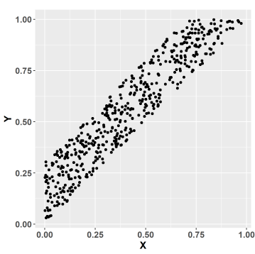
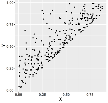
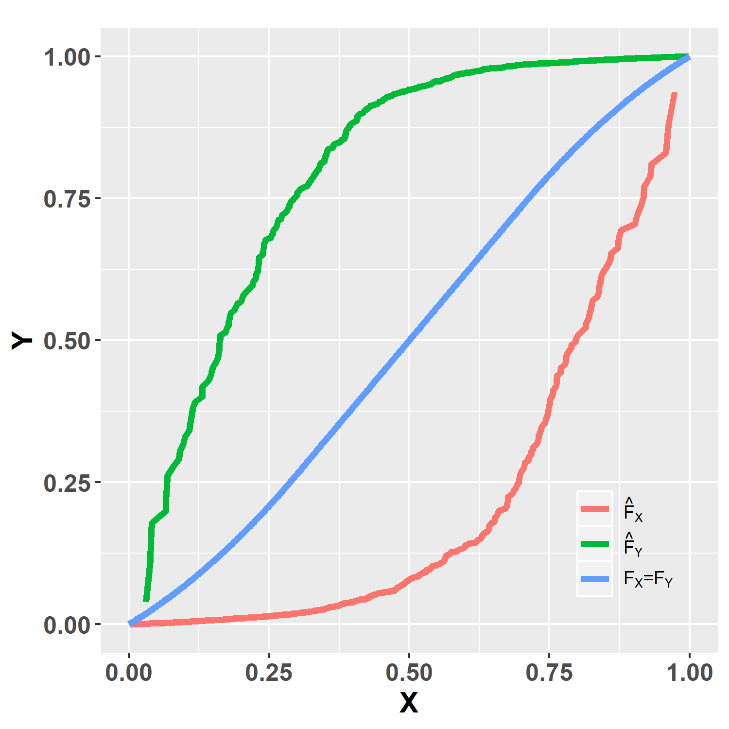
Figure 1: (left): a scatterplot of samples drawn from the true underlying distribution. (middle): a scatterplot of samples drawn from the truncated independence distribution, using the PL estimates. (right): the PL estimates of the univariate marginal CDFs $\hat{F}_{X}$ and $\hat{F}_{Y}$ are biased and do not resemble the true underlying CDF $F_{X}=F_{Y}$.

A possible solution is to find estimators for the marginal CDFs that are consistent also under the alternative hypothesis of quasi-dependence. However, as the model is not identifiable under the alternative (Cheng et al., 2007), such estimators can be calculated only under additional assumptions, either on ${w}(x,y)$, or on the underlying joint distribution (or both). We next demonstrate this through two different settings.

4.2.2 Case 2: Strictly Positive ${w}(x,y)>0$

The problem of estimating non-parametrically a general multivariate distribution $F$ using weighted data is well known (e.g., Vardi (1985)) and for $w>0$ the non-parametric maximum likelihood estimator (NPMLE) is given by:

$$\hat{F}_{XY}^{n}(t,s)=\frac{\sum_{i=1}^{n}\mathbbm{1}_{\{X_{i}\leq t,Y_{i}\leq s\}}w(X_{i},Y_{i})^{-1}}{\sum_{i=1}^{n}w(X_{i},Y_{i})^{-1}}.$$ (13)

Estimators for $F_{X}$ and $F_{Y}$ can be then obtained by marginalization of Equation (13),

$$\hat{F}_{X}^{n}(t)=\hat{F}_{XY}^{n}(x,\infty)=\frac{\sum_{i=1}^{n}\mathbbm{1}_{\{X_{i}\leq t\}}w(X_{i},Y_{i})^{-1}}{\sum_{i=1}^{n}w(X_{i},Y_{i})^{-1}}.$$ (14)

The estimator above can be used whenever $w>0$ in the entire support of $F_{XY}$. By the law of large numbers, $n^{-1}{\sum_{i=1}^{n}\mathbbm{1}_{\{X_{i}\leq t\}}w(X_{i},Y_{i})^{-1}}\to F_{X}(t)/\mathbb{E}_{f_{XY}}\{{w}(X,Y)\}$ a.s. and $n^{-1}{\sum_{i=1}^{n}w(X_{i},Y_{i})^{-1}}\to 1/\mathbb{E}_{f_{XY}}\{{w}(X,Y)\}$ a.s. so by the continuous mapping theorem $\hat{F}_{X}^{n}(t)\to F_{X}(t)$ a.s. By similar arguments, $\hat{F}_{Y}^{n}(s)\to F_{Y}(s)$ a.s.

4.2.3 Case 3: Left Truncation ${w}(x,y)=\mathbbm{1}_{\{x<y\}}$

In contrast to the former case, when ${w}(x,y)$ is a truncation function, estimating the marginals under quasi-independence is more challenging due to the actual loss of data and identifiability issues. Nevertheless, for certain types of truncation mechanisms, additional assumptions on the joint distribution may allow to reconstruct the marginals. In particular, the most familiar type of truncation in the statistical literature is left (or right) truncation, described by ${w}(x,y)=\mathbbm{1}_{\{x<y\}}$. The next proposition shows that under exchangeability, the empirical distribution function of the joint sample $X_{1},\ldots,X_{n},Y_{1},\ldots,Y_{n}$ is a consistent estimator for the marginals (the proof is in the Supp. Methods, Section A).

Proposition 1.

Let $F_{XY}(x,y)$ be an exchangeable joint distribution having a density $f_{XY}(x,y)\equiv f_{XY}(y,x)$ and let $\mathcal{D}\sim[F_{XY}^{(w)}]^{n}$ be a sample with the truncation weight function ${w}(x,y)=\mathbbm{1}_{\{x<y\}}$. Let $\hat{F}^{(w),n}_{X},\hat{F}^{(w),n}_{Y}$ be the empirical CDFs of $F_{X}^{(w)},F_{Y}^{(w)}$, respectively. Define:

$$\hat{F}_{X}^{n}(x)=\hat{F}_{Y}^{n}(x)=\frac{\hat{F}^{(w),n}_{X}(x)+\hat{F}^{(w),n}_{Y}(x)}{2}=\frac{1}{2n}\Big{[}\sum_{i=1}^{n}\mathbbm{1}_{\{X_{i}\leq x\}}+\sum_{i=1}^{n}\mathbbm{1}_{\{Y_{i}\leq x\}}\Big{]}.$$ (15)

Then $\hat{F}_{X}^{n},\hat{F}_{Y}^{n}\to F_{X}=F_{Y}$ a.s.

5 Test Statistics

5.1 The Adjusted Hoeffding Statistic

While the permutation and bootstrap approaches can be applied with any test statistic, our goal is to modify an existing omnibus test to weighted models in general and to truncation in particular. For the latter, most tests used to date are tailored to specific alternatives, such as monotone dependence. A recent new approach studied by Chiou et al. (2018) can test against a general alternative, but uses either significant computational resources or permutations with different sample sizes, so its significance level is not guaranteed. We are inspired by some popular non-parametric tests of independence such as Thas and Ottoy (2004), Heller et al. (2012), and Heller et al. (2016), and for concreteness, we describe the approach of the latter, which generalizes a modified version of Hoeffding (1948). Our problem requires two major modifications. First, biased sampling should be taken into account when computing the null distribution of the test statistic using a bootstrap or permutations resampling approach; this was addressed in the previous sections. Second, the test statistic compares observed counts with their expectations under the null, and the computation of these expectations needs to be modified to accommodate biased sampling.

The test belongs to a family of tests which compare the observed counts $o_{\mathcal{A}}$ to the expected counts $e_{\mathcal{A}}$ for different sets $\mathcal{A}\in\mathbb{R}^{2}$. As in Heller et al. (2016), our test statistic is based on Pearson’s Chi-squared statistics, and we consider all partitions defined by the data $\mathcal{D}$. Specifically, each data point $(x_{i},y_{i})\in\mathcal{D}$ defines a partition of $\mathbb{R}^{2}$ into four quadrants:

$$Q_{i}^{jk}\equiv\Big{\{}(x^{\prime},y^{\prime})\in\mathbb{R}^{2}\>:\>\mathbbm{1}_{\{x^{\prime}>x_{i}\}}=j,\mathbbm{1}_{\{y^{\prime}>y_{i}\}}=k\Big{\}}\quad j,k\in\{0,1\}.$$ (16)

For example, $Q_{i}^{00}=(-\infty,x_{i}]\times(-\infty,y_{i}]$ and $P\big{(}(X,Y)\in Q_{i}^{00}\big{)}=F_{XY}^{(w)}(x_{i},y_{i})$.

Let $(x_{i},y_{i})$ be a point in the sample $\mathcal{D}$. For a quadrant $Q_{i}^{jk}$, we denote the observed number of points by $o_{i}^{jk}\equiv o_{Q_{i}^{jk}}$ and the expected number of points under the null by $e_{i}^{jk}\equiv e_{Q_{i}^{jk}}$. We then compute, for each quadrant, the scaled squared difference between the observed and expected number of points under $H_{0}$. Finally, we sum over all the sample points to get our test statistic:

$$T=\sum_{i=1}^{n}\sum_{j,k\in\{0,1\}}\frac{(o_{i}^{jk}-e_{i}^{jk})^{2}}{e_{i}^{jk}}.$$ (17)

Estimating the expected values $e_{i}^{jk}$ requires the estimation of the null distribution, which may become highly non-trivial in the biased sampling setting. First, $F_{X}$ and $F_{Y}$ may be un-identifiable, and therefore using plug-in estimators of $F_{X},F_{Y}$ may give a poor approximation of the distribution of the test statistic under the null. Second, evaluation of expectations or probabilities under the null may require computationally costly integration of the null distribution, $[f_{X}f_{Y}]^{(w)}$, as opposed to a simple multiplication of the empirical marginals in the standard setting. If the expectations $e_{i}^{jk}$ are not estimated correctly, the WP test is still valid according to Corollary 1 and the bootstrap approach can be also applied, but power can be severely reduced, as is shown in the Supp. Materials, Section C.

5.1.1 Computing Expectations under Biased Sampling

A natural approach is to estimate the marginals $F_{X}$ and $F_{Y}$ under the null independence model and use them to calculate the expected count in a certain cell. However, as discussed in Section 4, this approach works well only for special models. We therefore suggest here an alternative method that directly estimates the expected counts.

Let $P_{ij}\equiv P_{\mathcal{W}}(\pi(i)=j)=\sum_{\pi\in S_{n}}P_{\mathcal{W}}(\pi)\mathbbm{1}_{\{\pi(i)=j\}}$, and define the Bernoulli random variables $\xi^{\pi}_{ij}\equiv\mathbbm{1}_{\{\pi(i)=j\}}$, so $P_{ij}=\mathbb{E}(\xi^{\pi}_{ij})$. Let $\mathcal{A}\subset\mathbb{R}^{2}$ be an arbitrary set. Given a sample $\mathcal{D}$, for any permutation $\pi$ of the data, denote the number of points in $\mathcal{A}$ under $\pi$ (i.e., after permuting the data set $\mathcal{D}$) by $o_{\mathcal{A}}(\pi)=\sum_{i=1}^{n}\mathbbm{1}_{\{(x_{i},y_{\pi(i)})\in{\mathcal{A}}\}}$, and let $e_{\mathcal{A}}\equiv\mathbb{E}_{P_{\mathcal{W}}}\{o_{\mathcal{A}}(\pi)\}$ be the expected number of data points in $\mathcal{A}$, under the permutations distribution $P_{\mathcal{W}}$.

The $P_{ij}$ values determine the expected number $e_{\mathcal{A}}$ for any set $\mathcal{A}$ via the following claim:

Claim 2.

For any $\mathcal{A}\subset\mathbb{R}^{2}$, the expected number of points $e_{\mathcal{A}}$ under the permutations distribution $P_{\mathcal{W}}$ is given by:

$$e_{\mathcal{A}}=\sum_{i,j=1}^{n}\mathbbm{1}_{\{(x_{i},y_{j})\in\mathcal{A}\}}\mathbb{E}_{P_{\mathcal{W}}}(\xi^{\pi}_{ij})=\sum_{i,j=1}^{n}\mathbbm{1}_{\{(x_{i},y_{j})\in\mathcal{A}\}}P_{ij}.$$ (18)

Proof.

By definition, we have:

$$e_{\mathcal{A}}=\mathbb{E}_{P_{\mathcal{W}}}\big{[}\sum_{i=1}^{n}\mathbbm{1}_{\{(x_{i},y_{\pi(i)})\in\mathcal{A}\}}\big{]}=\sum_{i,j=1}^{n}\mathbbm{1}_{\{(x_{i},y_{j})\in\mathcal{A}\}}P_{\mathcal{W}}\big{(}\pi(i)=j\big{)}=\sum_{i,j=1}^{n}\mathbbm{1}_{\{(x_{i},y_{j})\in\mathcal{A}\}}P_{ij}.$$ (19)

 

The probabilities $P_{ij}$ can be easily estimated using the MCMC scheme described in Algorithm 2: let $\pi_{0}$ be the identity permutation and $\pi_{1},..,\pi_{B}$ be the sampled permutations, and define the following estimator:

$$\hat{P}_{ij}\equiv\frac{1}{B+1}\sum_{b=0}^{B}\mathbbm{1}_{\{\pi_{b}(i)=j\}}.$$ (20)

When we sample permutations using an importance distribution $P_{IS}$ (see Section 3.4), the above estimator for ${P}_{ij}$ is replaced by:

$$\hat{P}_{ij}^{(IS)}\equiv\frac{\sum_{b=0}^{B}\mathbbm{1}_{\{\pi_{b}(i)=j\}}\frac{P_{\mathcal{W}}(\pi_{b})}{P_{IS}(\pi_{b})}}{\sum_{b=0}^{B}\frac{P_{\mathcal{W}}(\pi_{b})}{P_{IS}(\pi_{b})}}.$$ (21)

Plugging Equation (20) (or Equation (21)) into Equation (18) gives an estimator of $e_{\mathcal{A}}$,

$${\hat{e}}_{\mathcal{A}}=\sum_{i,j=1}^{n}\mathbbm{1}_{\{(x_{i},y_{j})\in\mathcal{A}\}}\hat{P}_{ij},$$ (22)

which can be used in the Chi-squared statistic.

For the bootstrap approach, the estimate of the null distribution is used in a straightforward manner. Consider, for example, the bottom-left quadrant with respect to a point $(x_{i},y_{i})$, $Q_{i}^{00}$; given estimators $\hat{F}_{X},\hat{F}_{Y}$ of the univariate CDFs, a natural estimator for the mass (up to a normalizing constant) that the null puts on $Q_{i}^{00}$ is given by

$$\widehat{e_{i}^{00}}=n[\hat{F}_{X}\hat{F}_{Y}]^{(w)}(x_{i},y_{i}).$$ (23)

5.2 An Inverse Weighting Statistic for Strictly Positive ${w}$

When ${w}$ is strictly positive, a test can utilize an inverse weighting approach. For a set $\mathcal{A}\in\mathbb{R}^{2}$, define the inverse weighted observed and expected counts $o_{\mathcal{A}}^{({w})}$ and $e_{\mathcal{A}}^{({w})}$, respectively:

$$o_{\mathcal{A}}^{({w})} =\sum_{\ell=1}^{n}\mathbbm{1}_{\{(x_{\ell},y_{\ell})\in\mathcal{A}\}}{w}(x_{\ell},y_{\ell})^{-1},$$

$$e_{\mathcal{A}}^{({w})} =nE_{[F_{X}F_{Y}]^{(w)}}\{\mathbbm{1}_{\mathcal{A}}{w}(X,Y)^{-1}\}.$$ (24)

For the quadrants $Q_{i}^{jk}$, we can compute estimates for the expected weighted counts ${e_{i}^{jk}}^{({w})}\equiv e_{Q_{i}^{jk}}^{({w})}$ by multiplying the corresponding marginal inverse weighted counts. For example, for $Q_{i}^{00}$:

$${e_{i}^{00}}^{({w})}=\frac{(\sum_{\ell=1}^{n}{w}(x_{\ell},y_{\ell})^{-1}\mathbbm{1}_{\{x_{\ell}\leq x_{i}\}})(\sum_{\ell=1}^{n}{w}(x_{\ell},y_{\ell})^{-1}\mathbbm{1}_{\{y_{\ell}\leq y_{i}\}})}{\sum_{\ell=1}^{n}{w}(x_{\ell},y_{\ell})^{-1}}.$$ (25)

Similarly to Equation (17), the weighted statistic is given by

$$T^{(w)}=\sum_{i=1}^{n}\sum_{j,k\in\{0,1\}}\frac{({o_{i}^{jk}}^{(w)}-{e_{i}^{jk}}^{(w)})^{2}}{{e_{i}^{jk}}^{(w)}}.$$ (26)

5.3 Unknown ${w}$: Left Truncated Right Censored Data

In some applications the biased sampling function ${w}$ is unknown. However, our methodology is still applicable when ${w}$ can be estimated consistently. In particular, we can tackle the important case of left truncation with censoring. Consider the standard left-truncation right-censoring model where $(X_{i},Y_{i},C_{i})$ are $n$ independent triplets, the joint density of $(X_{i},Y_{i})$ is proportional to $f_{XY}(x,y)\mathbbm{1}_{\{x<y\}}$ for some density $f_{XY}$, and $(X_{i},Y_{i})$ are independent of the censoring variables $C_{i}$. We observe triplets $(X_{i},\min(Y_{i},X_{i}+C_{i}),\Delta_{i}$), where $\Delta_{i}=\mathbbm{1}_{\{Y_{i}<X_{i}+C_{i}\}}$ are the censoring indicators with $\Delta_{i}=0$ and $1$ for censored and uncensored observations, respectively. We suggest testing independence based on the uncensored observations, where censored observations are used only for estimation of the weight function. Specifically, the conditional density of an uncensored observation is simply

$$\frac{S(y-x)f_{XY}(x,y)\mathbbm{1}_{\{x<y\}}}{\mathbb{E}_{f_{XY}}[S(Y-X)\mathbbm{1}_{\{X<Y\}}]},$$ (27)

where $S(t)=P(C>t)$ is the survival function of $C$. Thus, the density of uncensored observations has exactly the form of Equation (1), with $w(x,y)=\mathbbm{1}_{\{x<y\}}S(y-x)$, a function involving a continuous and a truncated part. The methods developed in previous sections are flexible enough to accommodate such functions. The survival function $S$ can be estimated by the standard Kaplan-Meier estimator applied to the data $\{(\min(C_{i},Y_{i}-X_{i}),1-\Delta_{i}),\>i=1,\ldots,n\}$.

6 Simulation Studies

We investigated, using simulation, the performances of the weighted permutation (WP) and bootstrap tests, and compared them to that of Tsai (1990)’s and the minimum $P_{value}$ (minP2) test of Chiou et al. (2018). The latter are applicable only to truncated data of the form ${w}(x,y)=\mathbbm{1}_{\{x<y\}}$.

We implemented the simulations in $R$, with time consuming parts implemented in c++ using the $rcpp$ package (Eddelbuettel et al. (2011)). Scripts reproducing all figures and tables are available online at https://github.com/YanivTenzer/TIBS. P-values for the minP2 test were calculated using the package permDep in R (Chiou, 2018), version $1.0.3$ (Aug. 14th, 2019) from https://github.com/stc04003/permDep.

We calculated the rejection rate (power) at a significance level $\alpha=0.05$ by averaging results of $500$ replications. As the tests are computationally demanding, we used small sample sizes of $n=100$ and $n=200$ observations for uncensored and censored settings, respectively, in order to perform extensive simulations under different settings. We used $B=1000$ permuted or bootstrap null datasets for all tests except minP2 for which we used only $B=100$ null datasets and $100$ replications, as it was much slower. The average running times of the tests on a standard laptop with an i7 2.8Ghz dual core Intel processor were $\approx\!0.02$ seconds for Tsai’s test, $\approx\!0.11$ seconds for the new weighted permutation test, $\approx\!2.86$ seconds for the bootstrap test and $\approx\!93.45$ seconds for the minP2 test.

6.1 Truncation, ${w}(x,y)=\mathbbm{1}_{\{x<y\}}$

We study the performances of the tests under truncation for various dependence models with and without censoring. The censoring variable, $C$, was sampled from Gamma distributions, with the shape and scale parameters set such that roughly $25\%-30\%$ of the observations were censored for each model.

We first simulated data under monotone dependence models with an exchangeable joint distribution, where consistent estimators of the marginals exist (as shown in Section 4) and we expect the bootstrap procedure to perform well. We generated $X$ and $Y$ from a standard bivariate Gaussian distribution with different correlations $\rho$ (Norm($\rho$)). In addition, we generated $X$ and $Y$ with standard Gaussian marginal distributions under two copula models: (i) The Gumbel copula (GC) with dependence parameter $\theta=1.6$ (Kendall’s $\tau=0.375$), and (ii) The Clayton copula (CC) with dependence parameter $\theta=0.5$ ($\tau=0.2$). Although both the Gumbel and Clayton copulas produce monotone dependence structures, the two are different in nature - while the former provides upper tail dependence structure the latter produces lower tail dependence (Nelsen, 2007). Figure 3 in the Supp. Materials presents scatterplots of simulated pairs from the three models.

The results are summarized in Table 1, with the test having the highest power shown in boldface. As expected, in the Gaussian settings, under the null distribution (i.e., $\rho=0$), all tests achieve the correct $\alpha=0.05$ error rate. Under the alternative, the bootstrap procedure demonstrates favorable performance in all three settings. In the Gaussian settings, for $\rho<0$ the WP test consistently outperforms minP2. The minP2 has the lowest power in this setting. For $\rho>0$, the WP test has poorer performance, probably due to the difficulty of sampling permutations consistent with the truncation, while Tsai’s test shows the second highest power, after the bootstrap.

		Uncensored ($n=100$)				Censored ($n=200$)
Setting	Model	Tsai	minP2	WP	Bootstrap	WP	MinP2	Tsai
Monotone Exchangeable	Norm($-0.9$)	1	1	1	1	1	1	1
	Norm($-0.7$)	0.998	0.960	0.998	1	1	0.828	1
	Norm($-0.5$)	0.764	0.510	0.742	0.998	0.813	0.284	0.895
	Norm($-0.3$)	0.284	0.130	0.278	0.828	0.273	0.096	0.366
	Norm($0.0$)	0.056	0.050	0.064	0.058	0.052	0.042	0.046
	Norm($0.3$)	0.178	0.110	0.118	0.780	0.097	0.083	0.202
	Norm($0.5$)	0.352	0.140	0.194	1	0.211	0.103	0.404
	Norm($0.7$)	0.498	0.290	0.262	1	0.389	0.097	0.729
	Norm($0.9$)	0.658	0.260	0.236	1	0.495	0.076	0.907
	GC ($\theta=1.6$)	0.196	0.130	0.104	1	0.079	0.080	0.192
	CC ($\theta=0.5$)	0.110	0.130	0.074	0.782	0.126	0.127	0.181
Monotone Non-Exchangeable	LD ($\rho=0.0)$	0.042	0.010	0.046	0.996	0.005	0.048	0.051
	LD ($\rho=0.4)$	0.634	0.330	0.578	0.704	0.060	0.056	0.250
Non-monotone Exchangeable	CLmix($0.5$)	0.278	0.140	0.412	0.338	0.398	0.120	0.308
Non-monotone, Non-exchangeable	CNorm($-0.9$)	0.992	1	1	1	1	0.987	0.897
	CNorm($-0.7$)	0.844	0.950	0.992	0.998	0.972	0.609	0.635
	CNorm($-0.5$)	0.514	0.600	0.794	0.988	0.626	0.262	0.321
	CNorm($-0.3$)	0.176	0.290	0.272	0.982	0.212	0.138	0.157
	CNorm($0.0$)	0.042	0.020	0.046	0.986	0.047	0.053	0.055
	CNorm($0.3$)	0.132	0.170	0.216	0.998	0.228	0.035	0.089
	CNorm($0.5$)	0.266	0.370	0.654	1	0.753	0.037	0.163
	CNorm($0.7$)	0.490	0.790	0.992	1	0.999	0.080	0.268
	CNorm($0.9$)	0.698	1	1	1	1	0.298	0.367

Table 1: Power at a significance level of $\alpha=0.05$ for left-truncated data (${w}(x,y)=\mathbbm{1}_{\{x<y\}}$) for uncensored (left 4 columns) and censored (right 3 columns) models. Norm($\rho$) - Bivariate normal distribution with correlation $\rho$. GC - The Gumbel Copula, CC - the Clayton Copula, with dependence parameter $\theta$. LD - Lifetime Distribution with correlation $\rho$, CLmix - an exchangeable mixture of two Clayton copulas, CNorm($\rho$) - non-exchangeable joint distribution with dependence parameter $\rho$.

Following Chiou et al. (2018), we next simulated data from a lifetime distribution (LD) where the joint distribution is non-exchangeable having marginal distributions $X\sim exp(5)$ and $Y\sim Weibull(3,8.5)$. We specified the dependence of $(X,Y)$ through a normal copula, where the strength of dependence is determined by the correlation parameter $\rho$. We simulated data under independent ($\rho=0$) and dependent ($\rho=0.4$) $F_{XY}$ before truncation. Figure 4 in the Supp. Materials displays scatterplots of simulated pairs from both models.

The results are shown in the second part of Table 1. Although $X$ and $Y$ are not exchangeable, we applied the bootstrap procedure (shown in light gray) as well, using marginal estimates according to Equation (15), in order to investigate the impact of model miss-specification on its performance. The devastating impact of model miss-specification under the null distribution for the bootstrap procedure is now apparent: the test does not retain the desired rejection rate $\alpha=0.05$ under the null hypothesis ($\rho=0$). For $\rho=0.4$, Tsai’s test has the highest power, followed by the WP test and then minP2.

The third simulation study evaluates the performance of the tests under non-monotone dependence. Starting with a non-monotone exchangeable model, we simulated data from a mixture of two Clayton copulas with dependence parameters $\theta=0.5\hskip 2.168pt(\tau=0.2)$ and $\theta=-0.5\hskip 2.168pt(\tau=-0.333)$, respectively, and equal population proportions. Figure 5 in the Supp. Materials presents scatterplots of simulated pairs from the model. The third part of Table 1 presents the results. Our bootstrap approach has the highest power, followed by the WP test, Tsai’s test and lastly minP2. It is somewhat surprising that Tsai’s test outperforms here minP2, as the former is tailored to monotone alternatives.

Finally, we considered a non-monotone and non-exchangeable model. We used a normal copula, CNorm($\rho$), with varied correlation coefficient $\rho$ to specify the joint distribution of $X$ and $Y$, where $X\sim Weibull(0.5,4)$ and $Y\sim U[0,16]$, set such that $\mathbb{E}(X)=\mathbb{E}(Y)=8$, and retained only pairs satisfying $Y\geq X$. Figure 6 in the Supp. Materials displays scatterplots of simulated pairs from the models. The last part of Table 1 presents the results. As expected, the bootstrap procedure (light gray) does not retain the desired rejection rate under the null hypothesis. Under the alternative, both the WP and minP2 tests outperform Tsai’s procedure across the entire range of the dependence parameter $\rho$. This behaviour is expected because both tests were designed to detect non-monotone dependency. Our method has the highest power for all values of $\rho$. minP2 is more powerful than Tsai’s test for strong (absolute) correlations and less powerful for weaker correlations.

6.2 Strictly Positive Bias Functions

Our new tests can be used to detect dependency in a general weighted model. To study the performance of our approach, we consider two cases of positive biased sampling. In the first case we took $w(x,y)=x+y$, where $X$ and $Y$ were sampled from the log-normal bivariate distribution with zero mean, unit variance and correlation $\rho$. Recall that for a strictly positive ${w}$, the inverse weighted Hoeffding statistic from Section 5.2 can be used as an alternative to the adjusted Hoeffiding statistic. We also compared here the bootstrap and MCMC approaches to the importance sampling approach from Section 3.4, with four different importance sampling distributions, described in the Supp. Methods, Section D. We applied six different sampling methods for p-value calculation for each of the two test statistics, resulting in twelve different tests. When applying the Bootstrap, we estimated the univariate marginals using the weighted estimators in Equation (14). Table 2 shows the rejection rates of the various tests at a significance level $\alpha=0.05$, for sample size $n=100$ and for $\rho=0$ (independence) and $\rho=0.2$. All tests except the bootstrap seem to maintain the significance level at approximately $\alpha=0.05$ under the null. Under the alternative, the importance sampling approach with a uniform and ’grid’ importance distribution is most powerful, but the MCMC approach is not far behind.

In the second example, we considered a bivariate Gaussian distribution $Norm(\rho)$ for $X$ and $Y$ as in Section 6.1, and with ${w}(x,y)\propto Norm(-\rho)$. The biased sampling function here masks the dependence so the observed pairs, $(X_{i},Y_{i})$, are independent Gaussian random variables. This example shows that biased sampling can not only create spurious dependencies, but can also mask true dependencies. Nevertheless, knowing ${w}$ we can apply our tests and detect the dependence, as is shown in Table 2. As expected, for all tests, as $\rho$ increases (we used only $\rho>0$ due to symmetry) the power increases quite rapidly. The importance sampling with a uniform distribution is usually the most powerful, with the MCMC approach very close or superior for strong correlation. The bootstrap approach shows poor performance for this case. As in the previous example, here too the inverse weighting statistic is inferior to the adjusted Hoeffding statistic. The relative success of the importance sampling schemes for both examples can be explained by the small sample size. As shown in the Supp. Materials, Section D, when the sample size increases the importance sampling distributions become unrepresentative of the distribution $P_{\mathcal{W}}$, resulting in poor performance, whereas the MCMC approach is much more robust to changes in sample size.

Model	WPIS	WPIS	WPIS	WPIS	WP	Bootstrap
IS-Dist.	Kou-McCullagh	Uniform	Monotone	Grid
LogNormal($\rho=0$)	0.048	0.050	0.016	0.050	0.056	0.072
IW	0.050	0.038	0.016	0.036	0.060	0.080
LogNormal($\rho=0.2$)	0.606	0.676	0.004	0.676	0.602	0.632
IW	0.384	0.432	0.000	0.428	0.382	0.414
Norm(0.0)	0.046	0.048	0.032	0.040	0.046	0.004
IW	0.056	0.058	0.032	0.054	0.050	0.004
Norm(0.1)	0.084	0.084	0.052	0.080	0.082	0.006
IW	0.076	0.076	0.032	0.076	0.078	0.008
Norm(0.3)	0.296	0.322	0.134	0.350	0.302	0.052
IW	0.282	0.296	0.136	0.318	0.298	0.024
Norm(0.5)	0.582	0.640	0.298	0.630	0.582	0.166
IW	0.502	0.526	0.228	0.532	0.492	0.038
Norm(0.7)	0.856	0.860	0.516	0.850	0.852	0.334
IW	0.730	0.706	0.456	0.684	0.726	0.078
Norm(0.9)	0.964	0.914	0.712	0.918	0.964	0.672
IW	0.876	0.800	0.662	0.786	0.878	0.114

Table 2: Strictly positive bias functions; estimated power at a significance level of $\alpha=0.05$, and sample size $n=100$ of the permutations (WP), uniform importance sampling permutations (WPIS), and bootstrap tests. For each parameter settings and sampling method two statistics were applied, shown in separate lines: The adjusted Hoeffding statistic, with expectations estimated using permutations/bootstrap samples, and the inverse weighting statistic (IW). The top four rows represent a LogNormal distribution with ${w}(x,y)=x+y$. The bottom rows represent a Gaussian distribution with correlation $\rho$, with $w(x,y)$ proportional to a Gaussian density with correlation $-\rho$.

7 Real-Life Datasets

$AIDS$	$Channing$ $House$
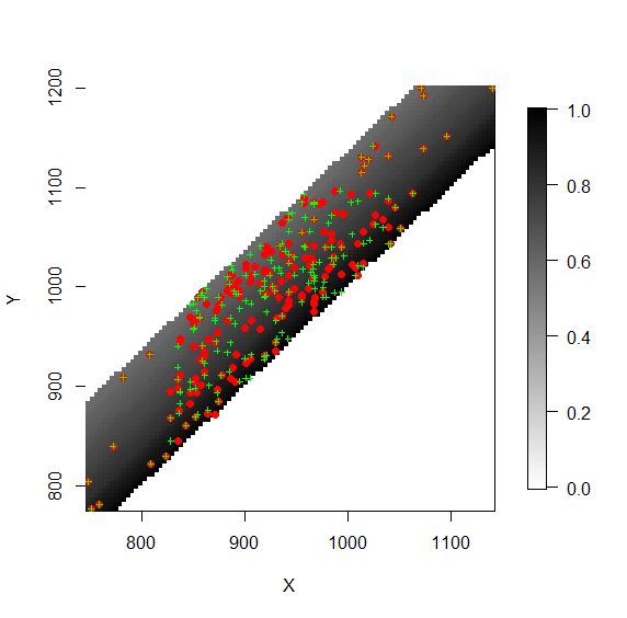
$Huji$	$Infection$

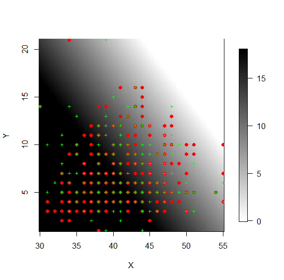
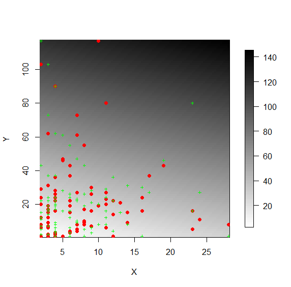
Figure 2: Scatterplots of four real datasets. Red points indicate the true data. Green ’+’ signs represent points $(x_{i},y_{\pi(i)})$ for randomly drawn permutations $\pi$ under biased sampling. The biased sampling functions are shown as background in grayscale, with ${w}(x,y)=\mathbbm{1}_{\{x<y\}}$ for the AIDS dataset, ${w}(x,y)=\mathbbm{1}_{\{x<y\}}S(y-x)$ for the Channing housing dataset, ${w}(x,y)=min(65−x-y,18)\mathbbm{1}_{\{x+y<65\}}$ for the Huji dataset and ${w}(x,y)=x+y$ for the Infection dataset.

We applied the various tests to four data sets, shown in Figure 2. P-values for the WP and bootstrap tests are based on $B=10^{5}$ samples, and for the minP2 test on $B=10^{4}$, due to computational restrictions.

1. Time from Infection to AIDS in HIV Carriers - A classical example of truncated data occur in AIDS retrospective studies, where the time from HIV infection to AIDS ($Y$) is restricted to be smaller than the time from HIV to sampling ($X$) (Lagakos et al., 1988). Here we analyze data on 295 AIDS cases, available in the DTDA package of R (Moreira et al., 2010). By design, the sample comprised only patients satisfying $0\leq X\leq Y$. The new WP, Tsai’s and minP2 tests all obtained significant P-values of $0.001$, $0.005$, and $0.002$, respectively, suggesting that dependence exists between the two time variables. To examine the effect of considering the truncation mechanism when testing for independence, we also performed a WP test with a constant ${w}$, and the P-value remained significant and in fact was reduced to $10^{-5}$.

2. Survival in the Channing House Community - Hyde (1977) analyzed survival data for residents of the Channing House retirement community in Palo Alto, CA; the full dataset is available in the boot $R$ package (Canty and Ripley, 2017). The survival time, $Y$, of a resident is left truncated by the entering age to the community, $X$, and is right censored by the age at the end of followup. After removing five observations that were not consistent with the criterion $X<Y$, the data consisted of $n=457$ individuals, 282 ($61.7\%$) of which were censored. Quasi independence of survival time and entering time was tested applying the approach described in Section 5.3. Tsai’s and minP2 tests were calculated for comparison. The WP, Tsai’s and minP2 tests all obtained non-significant P-values of $0.854$,  $0.099$ and $0.140$, respectively, showing no evidence for dependence between entering age and survival. As expected, when we ignored the truncation mechanism, a naive WP test of independence considering only the censoring and using ${w}(x,y)=S(y-x)$ (see Equation (27)) yielded a spurious signal of dependence, with a P-value of $10^{-5}$, demonstrating the need to account for biased sampling when testing.

3. Time before and after infection in Intensive-Care-Units - Data on $137$ patients that were hospitalized in Intensive-Care-Units (ICUs) on a random day were collected in five Israeli hospitals as part of a national cross-sectional study (Mandel, 2010). Infection data were collected from admission to the ICU until discharge or 30 days, whatever comes first. An important question was whether the time of infection is associated with the remaining time in the ICU. To test this independence hypothesis, we use the sub-sample of patients who admitted to the ICU without delay and who acquired infections during their first 30 days of hospitalization in the ICU. Thus, we test independence of $X$, the time from admission to the ICU to infection and $Y$, the time from infection to discharge from the ICU. Due to the sampling mechanism, the data are length biased according to the total length of stay in the ICU, yielding the weight function ${w}(x,y)=x+y$. The new WP and bootstrap tests were both significant at the standard $\alpha=0.05$ level, with P-values $0.039$ and $0.031$, respectively, indicating that the time of acquiring infection shows a significant effect on prolonging the remaining time in the ICU. When we used a WP test while ignoring the biased sampling function ${w}$, the signal for dependence disappeared, and we got a P-value of $0.605$. Thus, for this dataset the biased sampling masks the true dependence between $X$ and $Y$, and our test that takes ${w}$ into account was able to reveal it.

4. Time to Promotion to the Rank of Full Professor - The data consists of cross-sectional records on all faculty members of the Hebrew University of Jerusalem who were employed in $1998$. We tested whether the age at promotion to the associate professor rank depends on the service time in that rank. Let $A_{AP}$ and $A_{FP}$ denote the age at promotion to the ranks associate professor (AP) and full professor (FP) respectively; we test independence between $X=A_{AP}$ and $Y=A_{FP}−A_{AP}$ for associate professors promoted to full professor before the age of $65$, back then the retirement age in Israel. We used the sub-sample of $306$ faculty members who were promoted to the FP rank after 1980 and were younger than $65$ at sampling time (1998). As in Mandel and Rinott (2012), we assume that professors will stay in the university until age $65$. Assuming a stable entrance process to the AP rank, the cross-sectional study design leads to length biased sampling according to the length of service at the FP rank. The restriction of the data to professors who promoted after $1980$ resulted in the weight function ${w}(x,y)=\min(65−x-y,18)\mathbbm{1}_{\{x+y<65\}}$Thus, the weight is neither a truncation function nor strictly positive, and the only test applicable is the permutation test of Section 3.

   We applied the WP test with $B=10^{5}$ permutations, and obtained a very small P-value of $0.00002$, meaning that the age of promotion to associate professor rank does depend on the service time in that rank. Ignoring the biased sampling function ${w}$ still yielded a significant P-value of $0.00060$.

8 Discussion

In this paper we address the problem of testing quasi-independence in the presence of a general bias function and in possibly non-monotone settings. As demonstrated using real-life data sets, testing independence naively, while ignoring the bias function, can either create spurious dependence or mask true dependence.

We introduce two general machineries to simulate samples under the biased null distribution, namely, the permutations and bootstrap approaches, and examine the challenges possessed by both. Concretely, the former requires drawing permutations from a (general) non-uniform distribution, while the latter requires consistent estimation of the univariate marginals under the alternative hypothesis. We tackle the first challenge by utilising an MCMC scheme and an importance sampling methodology. Our simulation study indicates that for large sample size, the latter approach may suffer some degradation in performance, due to the difficulty in finding a proposal distribution suited for a general bias function.

On the bootstrap front, we identify two settings in which consistent estimators can be derived, both under the null and the alternative. We also introduce a new algorithm for estimating the marginal CDFs under the null, for a general bias function. This is of independent interest in cases where the null hypothesis is not rejected.

Importantly, both the permutations and bootstrap approaches can be combined with different statistics, thus result in a different test. As shown in simulations and real-life data sets, the choice of statistic can affect the power of the resulting test.

An appealing feature of the methodologies developed here is that they can be easily adapted to cases where the bias function is not known, but can be estimated from the data. An important instance of such cases is that of censoring. In particular, in observational studies, left truncation right censoring settings are frequently encountered. Our tests can accommodate such settings and it would be interesting to explore this approach further to more general cases of censoring and biased sampling.

We demonstrate the merit of our proposed tests, using simulated and real-life data sets, and showed that even for truncated data they attain similar and often higher power in most settings considered here, compared to the recent minP2 test.

Lastly, some theoretical aspects of the proposed algorithms are yet to be explored and left for future work. In particular we conjecture that, under the assumption of quasi-dependence, both the WP and bootstrap test are consistent.

Supplementary Materials

A Proofs

The proof of Claim 1 is brought below:

Proof.

For a general weighted model, we have

$$P(\pi(\mathcal{D})\mid x,\mathcal{D}_{y})=\frac{\prod_{i=1}^{n}f_{XY}^{(w)}(x_{i},y_{\pi(i)})}{\sum_{\pi^{\prime}\in S_{n}}\prod_{i=1}^{n}f_{XY}^{(w)}(x_{i},y_{\pi^{\prime}(i)})}.$$ (28)

Under the null, $f_{XY}^{(w)}(x,y)\propto w(x,y)\tilde{f_{X}}(x)\tilde{f_{Y}}(y)$, hence

$$P_{0}(\pi(\mathcal{D})\mid x,\mathcal{D}_{y})=\frac{\prod_{i=1}^{n}\tilde{f_{X}}(x_{i})\tilde{f_{Y}}(y_{\pi(i)})\mathcal{W}(i,\pi(i))}{\sum_{\pi^{\prime}\in S_{n}}\prod_{i=1}^{n}\tilde{f_{X}}(x_{i})\tilde{f_{Y}}(y_{\pi^{\prime}(i)})\mathcal{W}(i,\pi^{\prime}(i))}=P_{\mathcal{W}}(\pi).$$

 

The proof of Proposition 1 is brought below:

Proof.

Since $X$ and $Y$ are continuous exchangeable random variables, $P(X<Y)=1/2$ and therefore

$$f_{XY}^{(w)}(x,y)=2\mathbbm{1}_{\{x<y\}}f_{XY}(x,y).$$

Calculating the weighted marginal, we have

$$f_{X}^{(w)}(t)=2\int_{t}^{\infty}f_{XY}(t,y)dy=2\int_{t}^{\infty}f_{XY}(y,t)dy,$$

due to exchangeability. Similarly

$$f_{Y}^{(w)}(t)=2\int_{-\infty}^{t}f_{XY}(x,t)dx.$$

Thus (due to the continuity assumption),

$$\frac{f_{X}^{(w)}(t)+f_{Y}^{(w)}(t)}{2}=\int_{t}^{\infty}f_{XY}(y,t)dy+\int_{-\infty}^{t}f_{XY}(x,t)dx=f_{Y}(t).$$

The result follows by applying the Glivenko–Cantelli Theorem on $\hat{F}^{(w),n}_{X}$ and $\hat{F}^{(w),n}_{Y}$ .  

B Simulated Data

This section of the supplementary materials contains the estimated power and scatterplots for simulated data of the various settings presented in Section 6.

Monotone-Exchangeable Joint Distribution

$Norm(\rho=0.9)$	$Norm(\rho=-0.9)$	$GC(\theta=1.6)$	$CC(\theta=0.5)$

Figure 3: Scatterplots of $400$ samples generated from the monotone-exchangeable distributions described in Section 6.1 of the main manuscript, under truncation $\mathbbm{1}_{\{X\leq Y\}}$. Observed points are shown in red. Points excluded due to the truncation are shown in gray. All plots show data with standard Normal margins. The left two plots are for a bi-variate Gaussian distribution. For the negative correlation $(\rho=-0.9)$ the dependence between $X$ and $Y$ is immediately apparent even when observing only data after truncation. For the positive correlation $(\rho=0.9)$ the dependence is harder to detect by observing only such data, in similar to Figure LABEL:fig:example in the main text. The right two figures show data for the Gumbel copula (GC) with dependence parameter $\theta=1.6$ ,and the Clayton copula (CC) with dependence parameter $\theta=0.5$.

Figure  3 displays the scatterplots of samples generated from the monotone-exchangeable distributions described in Section 6.1 of the main manuscript. $X,Y$ were generated from a standard Gaussian distribution. We examined three possible dependence structures, as specified by three different copulas:

• Gaussian, with correlation parameter $\rho\in\{-0.9,-0.8,\ldots,0.9\}$

• Gumbel, with dependence parameter $\theta=1.6$

• Clayton, with dependence parameter $\theta=0.5$

Monotone Non-Exchangeable Joint Distribution

$LD(\rho=0)$	$LD(\rho=0.4)$

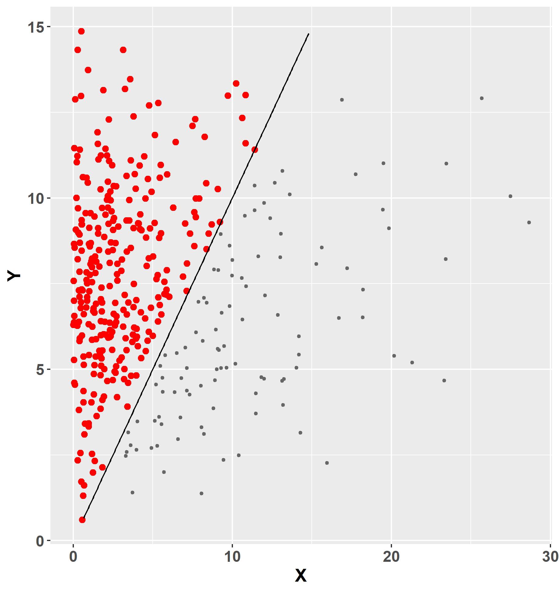
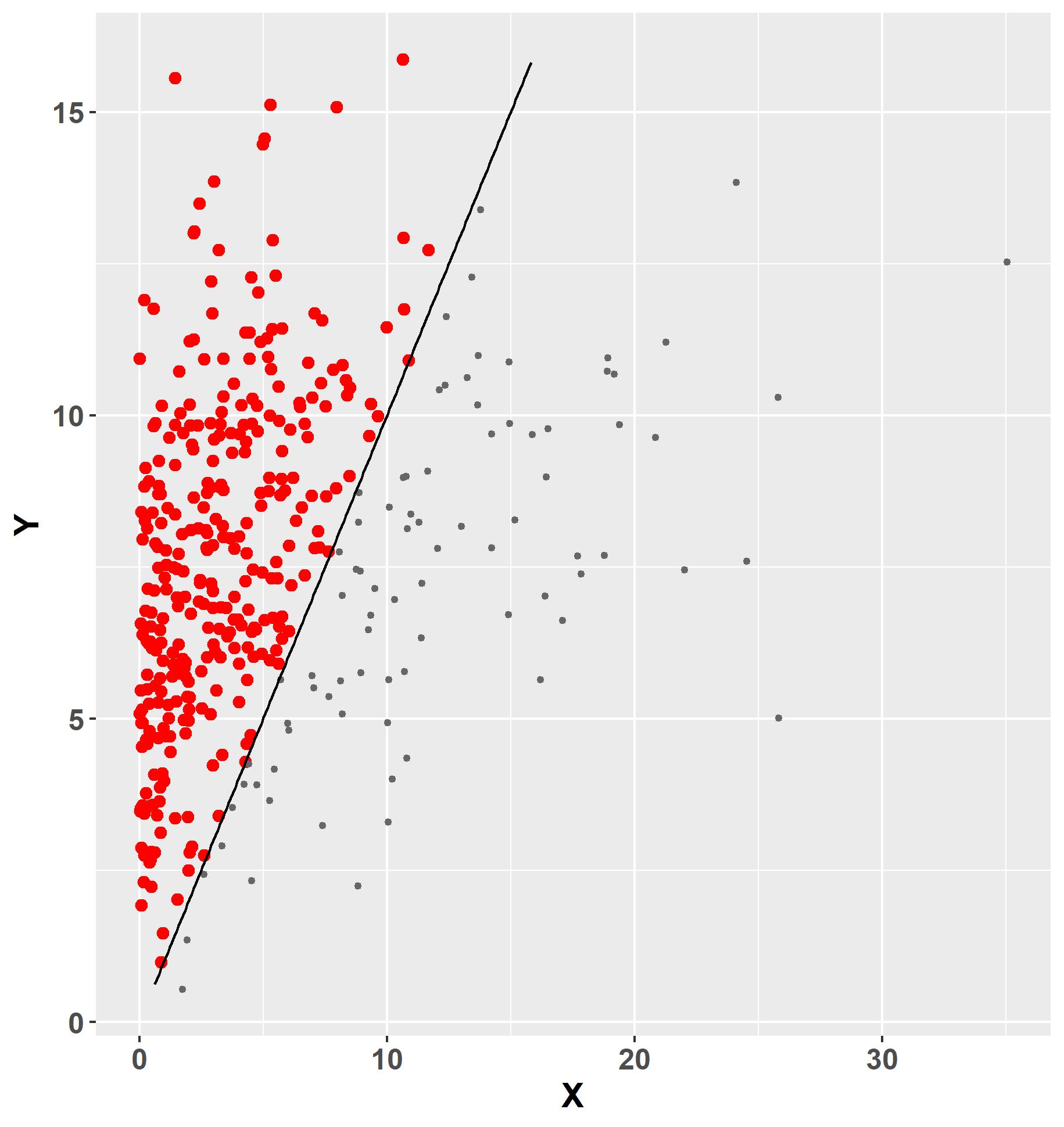
Figure 4: Scatterplots of samples generated from the monotone-non-exchangeable lifetime distribution (LD) described in Section 6.1 of the main manuscript, with otherwise the same settings as Figure 3. We used a Gaussian copula with dependence parameter $\rho=0$ (left) and $\rho=0.4$ (right), where $X\sim Weibull(8.5,3)$ and $Y\sim exp(0.2)$.

Figure  4 displays the scatterplots of samples generated from the monotone non-exchangeable distribution appear in Section 6.1 of the main manuscript. We generated pairs ($X,Y$) with $X\sim exp(0.2)$ and $Y\sim Weibull(3,8.5)$. We specified the dependence of $(X,Y)$ through a normal copula, where the strength dependence is determined by the correlation parameter $\rho$. We considered two levels of dependence as measured by the pre-truncation $\rho=0$ and $\rho=0.4$.

Non-Monotone Exchangeable Joint Distribution

$CLmix(0.5)$

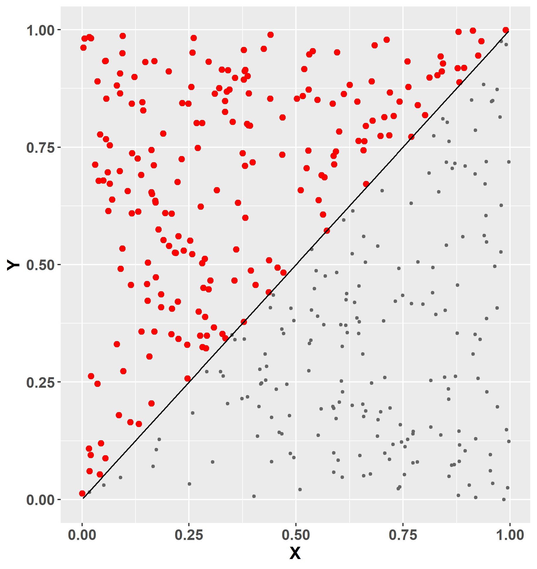
Figure 5: Scatterplots of samples generated from the non-monotone exchangeable distribution described in Section 6.1 of the main manuscript. $X,Y$ were generated from a mixture of two Clayton copulas with dependence parameters $\theta=0.5$ and $\theta=-0.5$.

Figure  5 displays the scatterplot of samples generated from the non-monotone exchangeable distribution described in Section 6.1 of the main manuscript. $X,Y$ were generated from a mixture of two Clayton copulas with dependence parameter $\theta=0.5$ and $\theta=-0.5$.

Non-Monotone Non-Exchangeable Joint Distribution

$CNorm(-0.9)$	$CNorm(0)$	$CNorm(0.5)$	$CNorm(0.9)$

Figure 6: Scatterplots of samples generated from the non-monotone non-exchangeable distributions described in Section 6.1. We used a normal copula with varied correlation coefficient $\rho$ to specify the joint distribution of $X,Y$, with $X\sim Weibull(0.5,4)$ and $Y\sim U[0,16]$. Due to the long tail of the Weibull distribution, we cut the $X$-axis at $40$, and points with $X_{i}>40$ are not shown.

Figure  6 displays the scatter plot of samples generated from the non-monotone non-exchangeable distributions described in Section 6.1. We used a normal copula with varied correlation coefficient $\rho$ to specify the joint distribution of $X,Y$, with $X\sim Weibull(0.5,4)$ and $Y\sim U[0,1]$.

B.1 Strictly Positive Biased Sampling

$LogNormal(\rho=0)$	$LogNormal(\rho=0.5)$	$LogNormal(\rho=0.9)$
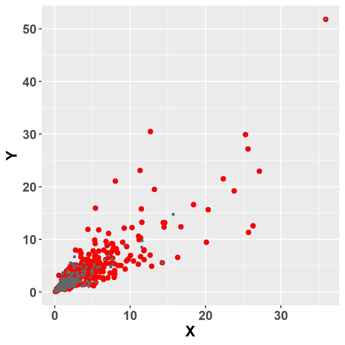
$Normal(\rho=0)$	$Normal(\rho=0.5)$	$Normal(\rho=0.9)$

Figure 7: Scatterplots of samples generated from distributions with positive biased sampling. Points sampled from $f_{XY}^{({w})}$ are shown in red. Points sampled from $f_{XY}$ are shown in gray. The top panels show data for the LogNormal distribution described in Section 6.2 of the main manuscript, sampled under the bias function ${w}(x,y)=x+y$ for different values of $\rho$. The sampling mechanism increases the values of the observed $(x_{i},y_{i})$ and creates spurious dependence even under the null ($\rho=0$). The bottom panels show data for the normal distribution with correlation $\rho$, sampled under a bias function proportional to the normal density with correlation $-\rho$. The sampling mechanism cancels the dependence between $X$ and $Y$ and the observed data is independent for all values of $\rho$.

Figure  7 displays the scatter plot of samples generated from the two distributions with positive biased sampling functions, described in Section 6.2 in the main text: (1.) A LogNorml distribution with standard marginals and correlation $\rho$ with ${w}(x,y)=x+y$, and (2.) a bi-variate Gaussian distribution with standard marginals and correlation $\rho$ with ${w}$ proportional to a bi-variate Gaussian density with standard marginals and correlation $-\rho$.

C Computing the Expectations for the Statistic Under the Null

Our two proposed tests are significantly faster than minP2, as shown in Section 6. However, Tsai’s test, which is specialized for truncation, is faster than our tests, especially compared to the bootstrap test which is about an order of magnitude slower than the weighted permutation test. It is thus natural to seek computational improvements for our tests, but this may have statistical, in addition to computational, consequences. In particular, the computation of our test statistic $T$ in Equation (17) requires estimation of the expected cell counts under the null $e_{i}^{jk}$. It is possible to use a different test statistic with different, albeit wrong, expectations. The weighted permutation test with this statistic will still be valid, according to Corollary 1, and a bootstrap test with this statistic can also be used. We examined two such modified statistics: (i) A naive approach, where we ignore the biased sampling function ${w}$ and simply use the empirical marginal distributions $\hat{F}_{X},\hat{F}_{Y}$ as our estimators, resulting the $T$ statistic used by Heller et al. [2012], and (ii) a fast bootstrap based approach, where the marginals are estimated according to Equation (23), but are not re-estimated for each bootstrap sample. While these two approaches appear simpler and are faster, they may suffer from significant loss of power. For example, for bivariate Gaussians with correlation coefficient $\rho=-0.4$, our bootstrap approach achieves a power of $0.634$, while using the naive expectations yield only power of $0.394$ and estimating the expectations only once via bootstrap achieves power of $0.406$. Similar trends of reduction in power were observed for other $\rho$ values.

D Algorithms for Importance Sampling

We have investigated several algorithms for importance sampling, and in particular their accuracy and validity for testing. In Chen and Liu [2007], a sequential importance sampling (SIS) algorithm for truncation was proposed. Kou and McCullagh [2009] generalized the algorithm for approximating the permanent and $\alpha$-permanent of general matrices. The validity of the importance sampling technique was established in Harrison [2012].

We describe in Algorithm 5 the details of the monotonic SIS scheme we have implemented. The idea behind this scheme is to order the rows $i$ of $\mathcal{W}$ in a decreasing order of the variance of the log-weights $\log(\mathcal{W}(i,j))$. Then, starting with the row with highest variance, for each such row $i$ select $\pi(i)$ maximizing $\log(\mathcal{W}(i,\pi(i)))$. This procedure will increase the value of $\log(\mathcal{W}(i,\pi(i)))$ for the first rows significantly beyond their expectation, where as we reach the last rows and must settle for lower values of $\log(\mathcal{W}(i,\pi(i)))$, the variance between different choices is small and the overall contribution to the product $P_{\mathcal{W}}(\pi)$ is not significant. As a result, this scheme samples permutations $\pi$ with high values of $P_{\mathcal{W}}(\pi)$. Additional algorithms can be suggested by small modifications of Algorithm 5. In ’uniform’ importance sampling, we simply sample permutations based on the uniform measure $P_{IS}(\pi)=\frac{1}{n!}$. The ’uniform grid’ method interpolates between the uniform method, that produce permutations with $P_{\mathcal{W}}(\pi)$ too low, and the monotonic method that produce permutations with $P_{\mathcal{W}}(\pi)$ that may be too high. This is achieved by taking a grid of values $0=\alpha_{1}<\alpha_{0}<..<\alpha_{G}=1$ and for each $\alpha_{k}$ modifying step $9$ of the algorithm to sample with probability proportional to $\mathcal{W}(\sigma(i),j)^{\alpha_{k}}$. In our simulations we used $G=10$ with equidistant $\alpha_{i}$ values. Finally, the Kou-McCullagh algorithm skips the ordering steps 5,6 and computes the column-sums $C_{i}=\sum_{j}\mathcal{W}(i,j)$ over the remaining rows at each step. Step $9$ is replaced by sampling $\pi(i,j)$ with probability proportional to $\frac{\mathcal{W}(i,j)}{C_{j}-\mathcal{W}(i,j)}$ (see Kou and McCullagh [2009] for more details).

We have studied the empirical performance of the SIS algorithms. To illustrate, we show their empirical rejection rate under the null for the LogNormal example with ${w}(x,y)=x+y$. While for $n=100$ the different sampling schemes perform reasonably well, as shown in Table 2, as the sample size $n$ grows, approximating the $P-value$ becomes more challenging. We illustrate the limitations of the algorithms in an example with $n=1000$. Empirically, the MCMC approach is robust and maintains an approximately uniform $U[0,1]$ P-values distribution under the null in all cases we have tested, while the importance sampling approaches are all overly conservative.

Figure 8 shows the probabilities of the sampled permutations under different methods, and the corresponding test statistic. Figure 9 shows the variability in the importance sampling weights $\frac{P_{\mathcal{W}}(\pi_{i})}{P_{IS}(\pi_{i})}$ of the different methods, causing a poor estimation of the P-value.

Figure 10 shows the resulting performance. The Kou-McCullagh scheme is the least conservative scheme among all SIS methods, but is still far from a uniform $U[0,1]$ P-values distribution. The power of the SIS under the alternative will also be reduced due to their conservative behaviour.

Algorithm 5 SIS Permutation Test of Quasi-Independence

1:Input: $\mathcal{D}$ - sample, ${w}(x,y)$ - bias function.

2:Parameters: $B$ - number of permutations.

3:Compute $\mathcal{W}(i,j)={w}(x_{i},y_{j}),\quad\forall i,j=1,..,n$.

4:Set $\pi_{0}$ the identity permutation $\pi_{0}(i)=i$.

5:for $b=1$ to $B$ do

6:    Initialize the importance sampling and weighted (unnormalized) probabilities            $\quad\quad P_{IS}(\pi_{b})=P_{\mathcal{W}}(\pi_{b})=1$.

7:    Compute $V_{i}=Var\Big{(}\log(\mathcal{W}(i,1)),..,\log(\mathcal{W}(i,n))\Big{)},\quad\forall i=1,..,n$.

8:    Order the variables by decreasing order of $V_{i}$: $V_{\sigma(1)}\geq...\geq V_{\sigma(n)}$.

9:    for $i=1$ to $n$ do

10:         Sample $\pi_{b}(\sigma(i))$ with probabilities:

11:                              $Pr(\pi_{b}(\sigma(i))=j)\propto\mathcal{W}(\sigma(i),j)\prod_{k=1}^{i-1}\mathbbm{1}_{\{\pi_{b}(\sigma(k))\neq j\}}$.

12:         Update the probability $P_{IS}(\pi_{b})=P_{IS}(\pi_{b})\times\frac{\mathcal{W}(\sigma(i),\pi_{b}(i))}{\sum_{j=1}^{n}\mathcal{W}(\sigma(i),j)\prod_{k=1}^{i-1}\mathbbm{1}_{\{\pi_{b}(\sigma(k))\neq j\}}}$ .

13:         Update the (unnormalized) probability $P_{\mathcal{W}}(\pi_{b})=P_{\mathcal{W}}(\pi_{b})\times\mathcal{W}(\sigma(i),\pi_{b}(i))$ .     

14:Output: $P_{value}$ computed from the $P_{IS}(\pi_{b}),P_{\mathcal{W}}(\pi_{b})$’s according to Equation (11).

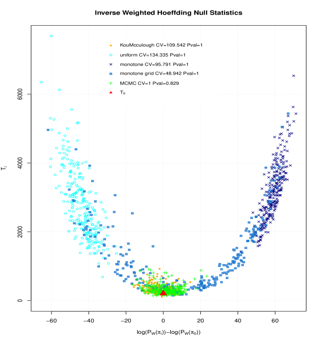
Figure 8: Log probabilities under $P_{\mathcal{W}}$ for permutations sampled under different methods, vs. their computed statistic $T_{i}=T(\pi_{i}(\mathcal{D}))$ for the inverse weighting statistic from Section 5.2. For $n=1000$, a weighted sample was simulated from the independent LogNormal distribution, with $\mathcal{W}(x,y)=x+y$. Since $P_{\mathcal{W}}$ is known only up to a multiplicative constant, we show the log probabilities minus the log probability of the identity permutation. Shown are the scaled log probabilities for $B=250$ random permutations for four importance sampling methods, and the MCMC method (green ’+’ signs), in addition to the ID permutation (red triangle). For each method, we also display the coefficient of variation diagnostic of $\frac{P_{\mathcal{W}}(\pi)}{P_{IS}(\pi)}$, and the resulting p-value. According to the MCMC Method, the permutations with log-probability close to the identity cover most of the probability space under $P_{\mathcal{W}}$. The uniform (monotone) importance sampling methods sample permutations with too low (high) $P_{\mathcal{W}}$ values. The monotone grid method interpolates between the two and covers a large range of the log-probabilities, including log-probabilities sampled under the MCMC method. The Kou-McCullagh method Kou and McCullagh [2009] also samples permutations with log-probabilities close to the MCMC method. However, the importance sampling probabilities $P_{IS}(\pi_{i})$ for the permutations sampled under these methods are vastly different from the true underlying probabilities $P_{\mathcal{W}}(\pi_{i})$, as is evident by the large value of the coefficient of variation $CV(\frac{P_{\mathcal{W}}(\pi_{i})}{P_{IS}(\pi_{i})})$. Although the true P-value is $\approx 0.24$ (as confirmed by extensive MCMC simulations with higher $B$), all importance sampling methods are too conservative here and give a P-value of $1$, in part due to the inclusion of the identity permutation in the P-value calculation.

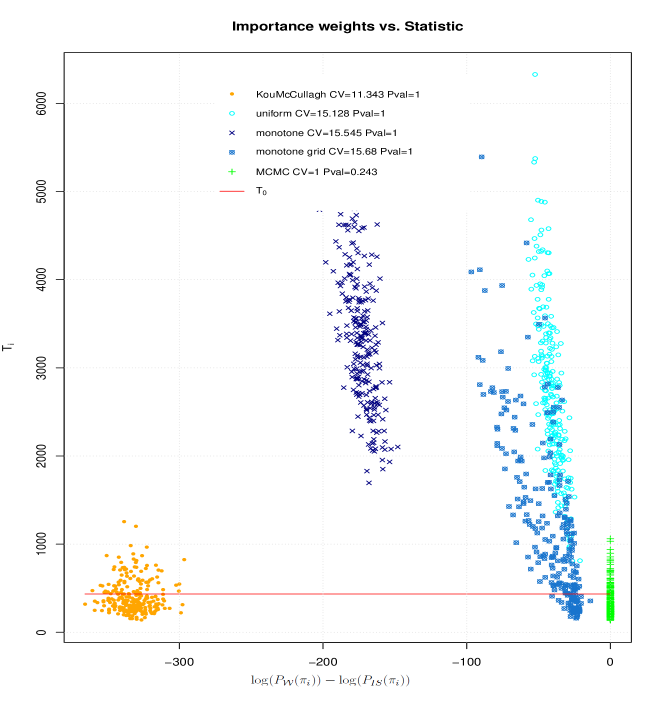
Figure 9: Log probabilities ratios $\log(\frac{P_{\mathcal{W}}}{P_{IS}})$ for permutations sampled under different methods, vs. their computed statistic $T_{i}=T(\pi_{i}(\mathcal{D}))$ for the inverse weighting statistic from Section 5.2. Parameters are the same as in Figure 8. Since $P_{\mathcal{W}}$ is known only up to a multiplicative constant, we show the log probabilities ratios minus the log probability ratio of the identity permutation. For the MCMC Method, the ratio is $1$ and all permutations have equal weights, with $\approx 24\%$ of permutations $\pi_{i}$ having $T_{i}\geq T_{0}$. For the uniform and monotone methods we have $T_{i}\geq T_{0}$ for all permutations giving a too conservative P-value of $1$. For the monotone-grid and Kou-McCullagh method, we do sample permutations with $T_{i}<T_{0}$, but their overall probabilities ratios are negligible, giving again a conservative $Pvalue\approx 1$.

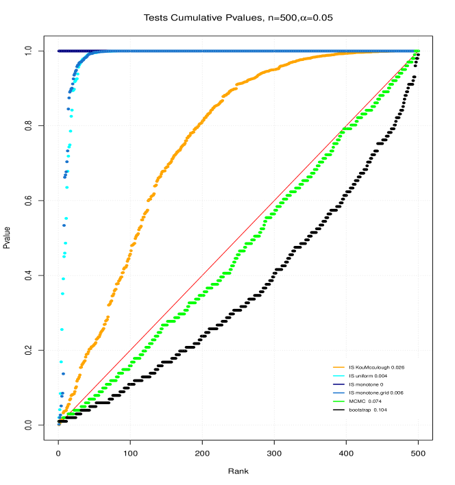
Figure 10: Cumulative p-value distribution for a the same independence LogNormal distribution from Figure 8 and the same tests. The permutation test gives an approximate $U[0,1]$ distribution. The bootstrap test is slightly non-calibrated, and gives low p-values under the null. The different importance sampling tests are all too conservative, with the Kou-McCullagh technique performing the best.

E An Iterative Algorithm for Marginal Estimation

This section deals with estimation of the marginal distributions under the null independence model presented in Section 4.2.1 in the main text. We consider the more general scenario of $k$ independent random variables ${X}_{1}\sim{F}_{1},\ldots,{X}_{k}\sim{F}_{k}$ that become dependent due to selection bias. Specifically, we assume that observations are vectors $(X_{1},\ldots,X_{k})$ having the density

$$\frac{w(x_{1},x_{2},\ldots,x_{k})F_{1}(dx_{1})F_{2}(dx_{2})\cdots F_{k}(dx_{k})}{\mathbb{E}\{w(X_{1},X_{2},\ldots,X_{k})\}},$$ (29)

where the non-negative weight function $w$ is known and has a finite expectation with respect to $F_{1}\times\cdots\times F_{k}$. The aim is to estimate $F_{1},\ldots,F_{k}$ without any parametric assumptions. For identifiability, we assume that for any measurable subset $\mathcal{A}$ in the support of $F_{j}$, ${E}\big{[}w(X_{1},\ldots,X_{k})\mathbbm{1}_{\{X_{j}\in\mathcal{A}\}}\big{]}>0$ ($j=1,\ldots,k$); that is, observations from any subset of the support can be observed.

The problem of non-parametric estimation of a general multivariate distribution $F$ using weighted data is well known (e.g., Vardi [1985]) and the corresponding estimator of $F_{1},\ldots,F_{k}$ can be obtained by marginalization. Specifically, generalizing Equation (13) in the main paper, the estimator for $F_{j}$ is

$$\hat{F}^{n}_{j}(t)=\frac{\sum_{i=1}^{n}I\{{X_{ij}\leq t}\}{w}(X_{i1},\ldots,X_{ik})^{-1}}{\sum_{i=1}^{n}{w}(X_{i1},\ldots,X_{ik})^{-1}}\quad(j=1,\ldots,k),$$ (30)

where $X_{i}$ is the vector of subject $i$, and $X_{ij}$ is its $j$’th coordinate. Estimator (30) does not exploit independence, and it is especially inappropriate when ${w}$ vanishes in part of the support (i.e., truncation).

Let ${\tilde{E}}$ denote the conditional expectation operator, ${\tilde{E}}(w;j,x)=\mathbb{E}\{w(X_{1},\ldots,X_{k})\mid X_{j}=x\}$. For any $1\leq j\leq k$, the likelihood of the data $(x_{i1},\ldots,x_{ik})$ ($i=1,\ldots,n$) can be factorized as follows (see Equation (29)):

$$\prod_{i=1}^{n}\frac{w(x_{i1},\ldots,x_{ik})\prod_{\ell\neq j}F_{i}(dx_{i\ell})}{{\tilde{E}}(w;j,x_{ij})}\times\prod_{i=1}^{n}\frac{{\tilde{E}}(w;j,x_{ij})F_{j}(dx_{ij})}{\mathbb{E}\{\tilde{E}(w;j,X_{j})\}}.$$ (31)

Due to independence, the first term in Equation (31) does not depend on $F_{j}$. Thus, assuming all distributions except $F_{j}$ are known, the likelihood of $n$ observations is proportional to the second term of Equation (31), and a natural non-parametric estimate of $F_{j}$ is $\hat{F}_{j}(x)\propto\sum_{i}\mathbbm{1}_{\{x_{ij}\leq x\}}{\tilde{E}}(w;j,x_{ij})^{-1}$. This estimator assigns mass only to the observed points and gives rise to Algorithm 6, generalizing Algorithm 4 in the main text.

Algorithm 6 Estimation of Marginals Under Quasi-independence

1:Input: $(x_{i1},\ldots,x_{ik})$ ($i=1,\ldots,n$) - sample, $w$ - bias function, $d(F_{1},F_{2})$ - distance function.

2:Parameters: $\epsilon$ - convergence criterion.

3:Generate initial estimates using Equation (30), and set $F^{new}_{j}=\hat{F}^{n}_{j}$, $F^{old}_{j}\equiv 0$.

4:while $\max_{j}d(F_{j}^{old},F_{j}^{new})<\epsilon$ do

5:    Set $F^{old}_{j}=F^{new}_{j}$ $(j=1,\ldots,k)$.

6:    for $j=1,\ldots,k$ do

7:         Calculate $e^{new}_{ij}={\tilde{E}}(w;j,x_{ij})$ with respect to $\prod_{\ell=1}^{k}F_{\ell}^{new}$, for all $x_{ij}$ $(i=1,\ldots,n)$.

8:         Set

$$F^{new}_{j}(x)=\frac{\sum_{i=1}^{n}\mathbbm{1}_{\{x_{ij}\leq x\}}[e^{new}_{ij}]^{-1}}{\sum_{i=1}^{n}[e^{new}_{ij}]^{-1}}.$$

    

9:Output: $F^{new}_{1},\ldots,F^{new}_{k}$.

Algorithm 6 provides a non-parametric estimator for the model under the independence constraint. The most time consuming part of the algorithm is the calculation of $e^{new}_{ij}={\tilde{E}}(w;j,x_{ij})$ in step 5. In most cases, it seems unavoidable to use full enumeration so the complexity of each step 5 is $O(n^{k})$. For the important case of a linear weight function, the calculation of ${\tilde{E}}(w;j,x_{ij})$ is rather simple. Let $w({\bf x})={\bf a}^{t}{\bf x}+b$, where the vector $\bf a$ and the constant $b$ are known ($\bf a\equiv 1$ and $b=0$ is the sum-bias case $w(\textbf{x})=x_{1}+\cdots+x_{k}$). Then

$${\tilde{E}}(w;j,x_{ij})={\bf a}^{t}\Big{(}\mathbb{E}(X_{1}),\ldots,\mathbb{E}(X_{j-1}),x_{ij},\mathbb{E}(X_{j+1}),\ldots,\mathbb{E}(X_{k})\Big{)}+b$$ (32)

where the expectations are calculated for each coordinate separately with respect to $F_{1}^{new},\ldots,F_{k}^{new}$. Thus, the computational complexity of each step $5$ reduces to $O(n)$.

Several properties of Algorithm 6 are readily established; their proofs are standard and hence are omitted.

Proposition 2.

The likelihood increases in each step of the algorithm.

Proposition 3.

The algorithm converges in the interior of the parameter space.

Proposition 4.

The NPMLE is a fixed point of the algorithm.

F Implementation Details

We list below several practical issues that were dealt with when implementing our TIBS algorithm.

• Permutations MCMC parameters: When sampling permutations, we seek permutations that are independent from each other. This is approximately achieved when enough MCMC steps are used between every two permutations chosen such that the Markov Chain is mixing and is close to the stationary distribution. The parameter $M$ of MCMC steps between two consecutive permutations was set to $M=2n$, where $n$ is the sample size. This choice was based on calculating the correlation between $\pi_{t}(i)$ and $\pi_{t+M}(i)$ as a function of $M$ and showing that this correlation decays.

  In addition, a ’burn-in’ parameter $M_{0}$ is often used in MCMC studies, which is the initial number of steps performed after starting from the identity permutation. Here, we chose to not include a ’burn-in’ step, i.e. setting $M_{0}=0$ and taking the first permutation (the identity) as one of our permutations. This ensures that under the null we have one sample identical to the original sample, i.e. the empirical p-value cannot be lower than $\frac{1}{B}$. Some empirical arguments against the usage of ’burn-in’ are given in http://users.stat.umn.edu/~geyer/mcmc/burn.html.

• Estimating expectations using MCMC: The MCMC permutations algorithm was used to estimate the expected cell counts in the test statistic, as shown in Equation (22), using the estimated transition probabilities $\hat{P}_{ij}$ in Equation (20). For these estimators, we used all permutations generated during the MCMC algorithm, and not only the $B$ permutations selected later to produce permuted (null) samples. While consecutive permutations are strongly dependent and differ only in one pair ($\pi(i),\pi(j)$), adding the estimator for $P_{ij}$ over all permutations reduces the variance of the expected cell estimators, compared to using only every $M$’th permutation, at a negligible additional computational cost.

• Removing cells with low counts: The test statistic $T$ in Equation (17) sums over all cells, including cells with small expected counts. Such cells yield terms with high variance and may therefore reduce the power of the test statistic, especially recalling that we have variance not only in the observed counts $o_{i}^{jk}$ but we also use estimators $\hat{e}_{i}^{jk}$ for the expected counts.

  To reduce the variance of these cells, we include in the test statistic the contribution of cells for a data point $i$ only if $\hat{e}_{i}^{jk}>1$ for all $j,k$. Otherwise, we simply skip these cells, for both the original sample and the permuted and bootstrap samples. Alternatively, one can replace the Pearson chi-square statistic by a likelihood-ratio test statistic that is less sensitive to cells with low counts.

• Dealing with ties: Even for a continuous distribution $F_{XY}$ and for our test statistic $T$ in Equation (17), we encounter ties data points $(x_{i},y_{i})$ determining the quadrants $Q_{i}^{jk}$ and data points $(x_{j},y_{\ell})$ used as counts for the statistic. When $x_{j}=x_{i}$ and/or $y_{\ell}=y_{i}$ the data points lie on the boundaries of the quadrants $Q_{i}^{jk}$. This can occur in the bootstrap test (as the same values may be sampled multiple times), and also for permutation testing, where the permuted sample contains data points $(x_{i},y_{\ell})$ and $(x_{j},y_{i})$ for some $j,{\ell}$. We can count these boundary points on one quadrant, another, or ignore them altogether. While the effect of such ties is asymptotically negligible - they may affect the statistic and P-value calculation for small samples. For example, if we discard them, then for the original sample the sum of the four quadrants observed counts will be $n-1$, but for a permuted dataset this will be typically $n-2$. This causes a small but systematic bias between the original and randomized (permuted or bootstrap) samples, and may result in an invalid test with a non-uniform P-values distribution under the null. To overcome this bias, our implementation uses a small perturbation of the quadrants $Q_{i}^{jk}$ (see Equation (16)), such that the center point used is $(x_{i}+\epsilon^{(x)}_{i},y_{i}+\epsilon^{(y)}_{i})$ with $\epsilon^{(x)}_{i},\epsilon^{(y)}_{i}\overset{i.i.d.}{\sim}N(0,10^{-9})$. This randomly assigns any point (in the original or bootstrap/permuted sample) containing $x_{i}$ or $y_{i}$ (for example the original data point $(x_{i},y_{i})$) into one of the relevant quadrants, and does not affect the assignment of other points, thus ensuring that all $n$ points are counted for both the original and the randomized samples.

References

- Bickel and Ritov [1991] P.J. Bickel and J. Ritov. Large sample theory of estimation in biased sampling regression models. i. The Annals of Statistics, pages 797–816, 1991.
- Canty and Ripley [2017] A. Canty and B.D. Ripley. boot: Bootstrap R (S-Plus) Functions, 2017. R package version 1.3-20.
- Chen et al. [1996] C-H. Chen, W-Y. Tsai, and W-H. Chao. The product-moment correlation coefficient and linear regression for truncated data. Journal of the American Statistical Association, 91(435):1181–1186, 1996.
- Chen and Liu [2007] Y. Chen and J. S. Liu. Sequential monte carlo methods for permutation tests on truncated data. Statistica Sinica, pages 857–872, 2007.
- Cheng et al. [2007] M-Y. Cheng, P. Hall, and Y-J. Yang. Nonparametric inference under dependent truncation. Acta Scientiarum Mathematicarum, 73(1-2):397–422, 2007.
- Chiou [2018] S.H. Chiou. permDep: Permutation Tests for General Dependent Truncation, 2018. URL https://CRAN.R-project.org/package=permDep. R package version 1.0.2.
- Chiou et al. [2018] S.H. Chiou, J. Qian, E. Mormino, R.A. Betensky, Lifestyle Flagship Study of Aging, Harvard Aging Brain Study, Alzheimer’s Disease Neuroimaging Initiative, et al. Permutation tests for general dependent truncation. Computational Statistics & Data Analysis, 128:308–324, 2018.
- de Uña-Álvarez [2012] J. de Uña-Álvarez. On the markov three-state progressive model. In Recent Advances in System Reliability, pages 269–281. Springer, 2012.
- Diaconis et al. [2001] P. Diaconis, R. Graham, and S.P. Holmes. Statistical problems involving permutations with restricted positions. Lecture Notes-Monograph Series, pages 195–222, 2001.
- Eddelbuettel et al. [2011] D. Eddelbuettel, R. François, J. Allaire, K. Ushey, Q. Kou, N. Russel, J. Chambers, and D. Bates. Rcpp: Seamless r and c++ integration. Journal of Statistical Software, 40(8):1–18, 2011.
- Efron and Petrosian [1999] B. Efron and V. Petrosian. Nonparametric methods for doubly truncated data. Journal of the American Statistical Association, 94(447):824–834, 1999.
- Elderton et al. [1913] E.M. Elderton, A. Barrington, H. G. Jones, E. Lamotte, H. Laski, and K. Pearson. On the correlation of fertility with social value. A Cooperative Study, 3, 1913.
- Emura and Wang [2010] T. Emura and W. Wang. Testing quasi-independence for truncation data. Journal of Multivariate Analysis, 101(1):223–239, 2010.
- Goodman [1968] L.A. Goodman. The analysis of cross-classified data: Independence, quasi-independence, and interactions in contingency tables with or without missing entries: Ra fisher memorial lecture. Journal of the American Statistical Association, 63(324):1091–1131, 1968.
- Gretton et al. [2008] A. Gretton, K. Fukumizu, C.H. Teo, L. Song, B. Schölkopf, and A.J. Smola. A kernel statistical test of independence. In Advances in neural information processing systems, pages 585–592, 2008.
- Harrison [2012] M.T. Harrison. Conservative hypothesis tests and confidence intervals using importance sampling. Biometrika, 99(1):57–69, 2012.
- Hastings [1970] W.K. Hastings. Monte carlo sampling methods using markov chains and their applications. 1970.
- Heller et al. [2012] R. Heller, Y. Heller, and M. Gorfine. A consistent multivariate test of association based on ranks of distances. Biometrika, 100(2):503–510, 2012.
- Heller et al. [2016] R. Heller, Y. Heller, S. Kaufman, B. Brill, and M. Gorfine. Consistent distribution-free k-sample and independence tests for univariate random variables. Journal of Machine Learning Research, 17(29):1–54, 2016.
- Hoeffding [1948] W. Hoeffding. A non-parametric test of independence. The annals of mathematical statistics, pages 546–557, 1948.
- Hyde [1977] J. Hyde. Testing survival under right censoring and left truncation. Biometrika, 64(2):225–230, 1977.
- Kou and McCullagh [2009] S.C. Kou and P. McCullagh. Approximating the -permanent. Biometrika, 96(3):635–644, 2009.
- Lagakos et al. [1988] S.W. Lagakos, L.M. Barraj, and V. de Gruttola. Nonparametric analysis of truncated survival data, with application to aids. Biometrika, 75(3):515–523, 1988.
- Mandel [2010] M. Mandel. The competing risks illness–death model under cross-sectional sampling. Biostatistics, 11(2):290–303, 2010.
- Mandel and Rinott [2012] M. Mandel and Y. Rinott. Cross-Sectional Sampling, Bias, Dependence, and Composite Likelihood. Center for the Study of Rationality, 2012.
- Martin and Betensky [2005] E.C. Martin and R.A. Betensky. Testing quasi-independence of failure and truncation times via conditional kendall’s tau. Journal of the American Statistical Association, 100(470):484–492, 2005.
- Metropolis et al. [1953] N. Metropolis, A.W. Rosenbluth, M.N. Rosenbluth, A.H. Teller, and E. Teller. Equation of state calculations by fast computing machines. The journal of chemical physics, 21(6):1087–1092, 1953.
- Moreira et al. [2010] C. Moreira, J. de Uña-Álvarez, R. Crujeiras, et al. Dtda: an r package to analyze randomly truncated data. Journal of Statistical Software, 37(i07), 2010.
- Nelsen [2007] R.B. Nelsen. An introduction to copulas. Springer Science & Business Media, 2007.
- Rodríguez-Girondo and de Uña-Álvarez [2012] M. Rodríguez-Girondo and J. de Uña-Álvarez. A nonparametric test for markovianity in the illness-death model. Statistics in medicine, 31(30):4416–4427, 2012.
- Rodríguez-Girondo and de Uña-Álvarez [2016] M. Rodríguez-Girondo and J. de Uña-Álvarez. Methods for testing the markov condition in the illness–death model: a comparative study. Statistics in medicine, 35(20):3549–3562, 2016.
- Székely et al. [2009] G.J. Székely, M.L. Rizzo, et al. Brownian distance covariance. The Annals of Applied Statistics, 3(4):1236–1265, 2009.
- Thas and Ottoy [2004] O. Thas and J-P. Ottoy. A nonparametric test for independence based on sample space partitions. Comm. in Statistics-Simulation and Computation, 33(3):711–728, 2004.
- Tsai [1990] W-Y. Tsai. Testing the assumption of independence of truncation time and failure time. Biometrika, pages 169–177, 1990.
- Vardi [1985] Y. Vardi. Empirical distributions in selection bias models. The Annals of Statistics, 13(1):178–203, 1985.