From Polarimetry to Helicity: Studies of Solar Magnetic Fields at the Huairou Solar Observing Station

Abstract

In this paper, we briefly introduce the basic questions in the measurements of solar magnetic fields and the possible error sources due to the approximation of the theory of radiation transfer of spectral lines in the solar atmosphere. We introduce some basic research progress in magnetic field measurement at Huairou Solar Observing Station of National Astronomical Observatories of the Chinese Academy of Sciences, especially concerning the non-potentiality in solar active regions, such as the magnetic shear, current and helicity. We also discuss some basic questions for the measurements of the magnetic fields and corresponding challenges for the future studies.

1 Introduction

Since the 80s of the last century, a series of solar vector magnetograms have been observed at Huairou Solar Observing Station of National Astronomical Observatory of the Chinese Academy of Sciences. These observations present a large mount of information on the solar magnetic activities, including the basic structure, evolution of the magnetic field, the formation of the non-potential magnetic field, the current and also the corresponding helicity in solar active regions.

It is noticed that our research of solar magnetic fields is usually based on the theory of radiation transfer in the solar magnetic atmosphere. This implies that the general information of the solar photospheric vector magnetic field and the chromospheric magnetic field is based on the measurement of polarized light by means of the Zeeman effect. The study of the line formation in solar magnetic atmosphere not only provides a basic estimation for understanding the accuracy of the measured solar magnetic field, but also the base of the theoretical analysis of the solar magnetic fields. This leads us need to know the possible sources of errors or deviations obtained from these magnetic field observations, even if the errors caused by optical instruments have been ignored.

In this paper, we try to review, examine and analyze some background of solar magnetic field research based on magnetic field data obtained at Huairou Solar Observing Station, and highlighting some scientific achievements. We only briefly discuss some of the topics concerning fundamental questions from observations of solar magnetic fields, and do not give references to all aspects. Nevertheless, there are still some fundamental questions remained and to be researched in the future.

2 General Description of Radiative Transfer

The radiative transfer of the magnetically sensitive lines in solar atmosphere is a complex process. The diagnostic of solar magnetic fields based on these magnetically sensitive lines normally accompanies with some assumptions and approximations of the theoretical analysis, which probably are some error sources of the inversion of solar magnetic fields from observations. The important is to prevent or avoid the influence of these errors and trying to obtain relative accurated information of solar magnetic fields. As the relevant forms of the solution of the radiative transfer equations have been used to detect the solar magnetic fields, the corresponding spectral line formation in solar magnetic fields need to be analyzed in more detail.

In the stellar magnetic atmosphere, the non local thermodynamic equilibrium (non-LTE) equation of Stokes vector ${\textbf{ I}_{\nu}}=(I_{\nu},Q_{\nu},U_{\nu},V_{\nu})$ for the transfer of polarized radiation can be written in a general matrix form (Stenflo (1994) [1])

$$\frac{d\textbf{ I}_{\nu}}{ds}=-(N_{J_{l}}B_{J_{l}J_{u}}\Phi_{J_{l}}-N_{J_{u}}B_{J_{u}J_{l}}\Phi_{J_{u}})\frac{h\nu}{4\pi}\textbf{ I}_{\nu}+\textbf{ j},$$ (1)

where in the case of non-scattering process the emission vector is approximately by

$$\textbf{ j}=\frac{h\nu}{4\pi}\Phi_{J_{u}}\textbf{ 1}N_{J_{u}}A_{J_{u}J_{l}},$$ (2)

and the relationship with

$$A_{ji}=\frac{2h\nu^{3}}{c^{2}}B_{ji},~{}~{}~{}N_{i}C_{ij}=N_{j}C_{ji},$$ (3)

$$\frac{C_{ij}}{C_{ji}}=\frac{g_{j}}{g_{i}}e^{E_{ij}/kT}~{}~{}~{}\mathrm{and}~{}~{}~{}g_{j}B_{ji}=g_{i}B_{ij},$$ (4)

where $B_{ij}$, $B_{ji}$ and $A_{ji}$ are Einstein coefficients, $C_{ij}$ and $C_{ji}$ are collisional coefficients [2, 3]. Non-LTE population departure coefficients $b_{i}$ are defined as:

$$b_{l}=N_{l}/N^{LTE}_{l},~{}~{}~{}b_{u}=N_{u}/N^{LTE}_{u}$$ (5)

with $N_{(l,u)}$ the actual population and $N^{LTE}_{(l,u)}$ the Saha-Boltzmann values for the lower and upper levels, respectively. The expanded form of ${\Phi}$ is the matrix in the right-hand side of Eq. (7), and we introduce the source function in the form

$$S_{\nu}=\frac{N_{j}A_{ji}}{N_{i}B_{ij}-N_{j}B_{ji}}.$$ (6)

When we study the formation of polarized light in the magnetic field with Stokes parameters, Unno-Rachkovsky equations of polarized radiative transfer of spectral lines can be taken the form (Unno (1956) [4] and Rachkovsky (1962a, b) [5, 6])

$$\mu\frac{d}{d\tau_{c}}\left(\begin{array}[]{c}I\\ Q\\ U\\ V\end{array}\right)=\left(\begin{array}[]{cccc}\eta_{0}+\eta_{I}&\eta_{Q}&\eta_{U}&\eta_{V}\\ \eta_{Q}&\eta_{0}+\eta_{I}&\rho_{V}&-\rho_{U}\\ \eta_{U}&-\rho_{V}&\eta_{0}+\eta_{I}&\rho_{Q}\\ \eta_{V}&\rho_{U}&-\rho_{Q}&\eta_{0}+\eta_{I}\end{array}\right)\left(\begin{array}[]{c}I-S\\ Q\\ U\\ V\end{array}\right).$$ (7)

The symbols have their usual meanings given by Landi Degl’Innocenti (1976) [13]. In Eqs. (7), $d\tau_{c}=-\kappa_{c}ds$, and $\eta_{I}$, $\eta_{Q}$, $\eta_{U}$, $\eta_{V}$ are Stokes absorption coefficient parameters and $\rho_{Q}$, $\rho_{U}$ and $\rho_{V}$ are related to the magneto-optical effects.

In the analytical solution of the radiative transfer equations for polarized spectral lines [4, 5, 6], several limitations are introduced: (a) Uni-dimensional plane-parallel atmosphere with a constant magnetic field; (b) linear dependence of the source function with optical depth; (c) constant ratio of the line and continuous absorption coefficients. The transfer equations for polarized radiation can be solved to give

$$I = S\!_{0}+\mu S\!_{1}\triangle^{-1}[(1+\eta_{I})((1+\eta_{I})^{2}+\rho_{Q}^{2}+\rho_{U}^{2}+\rho_{V}^{2})],$$

$$Q = -\mu S\!_{1}\triangle^{-1}[(1+\eta_{I})^{2}\eta_{Q}+(1+\eta_{I})(\eta_{V}\rho_{U}-\eta_{U}\rho_{V})$$

$$+\rho_{Q}(\eta_{Q}\varrho_{Q}+\eta_{U}\varrho_{U}+\eta_{V}\varrho_{V})],$$

$$U = -\mu S\!_{1}\triangle^{-1}[(1+\eta_{I})^{2}\eta_{U}+(1+\eta_{I})(\eta_{Q}\rho_{V}-\eta_{V}\rho_{Q})$$

$$+\rho_{Q}(\eta_{Q}\varrho_{Q}+\eta_{U}\varrho_{U}+\eta_{V}\varrho_{V})],$$

$$V = -\mu S\!_{1}\triangle^{-1}[(1+\eta_{I})^{2}\eta_{V}+\rho_{V}(\eta_{Q}\varrho_{Q}+\eta_{U}\varrho_{U}+\eta_{V}\varrho_{V})].$$

where

$$\triangle = (1+\eta_{I})^{2}[(1+\eta_{I})^{2}-\eta_{Q}^{2}-\eta_{U}^{2}-\eta_{V}^{2}+\rho_{Q}^{2}+\rho_{U}^{2}+\rho_{V}^{2}]$$

$$-(\eta_{Q}\varrho_{Q}+\eta_{U}\varrho_{U}+\eta_{V}\varrho_{V})^{2},$$

and where the source function $S(\tau)=S\!_{0}+S\!_{1}\tau$.

In the approximation of the weak magnetic field (Stix, 2002) [14], one can obtain the following formulas

$$\eta_{I} = \eta_{p}+O(v_{b}^{2}),$$

$$\eta_{Q} = -\frac{1}{4}\frac{\partial^{2}\eta_{p}}{\partial v^{2}}v_{b}^{2}\sin^{2}\psi\cos 2\varphi+O(v^{4}_{b}),$$ (9)

$$\eta_{U} = -\frac{1}{4}\frac{\partial^{2}\eta_{p}}{\partial v^{2}}v_{b}^{2}\sin^{2}\psi\sin 2\varphi+O(v^{4}_{b}),$$

$$\eta_{V} = \frac{\partial\eta_{p}}{\partial v}v_{b}\cos\psi+O(v^{3}_{b}),$$

where $v_{b}=\bigtriangleup\lambda_{b}/\!\bigtriangleup\!\lambda_{D}$, and $\bigtriangleup\lambda_{b}$ is the corresponding splitting of different subcomponents of the magneto-sensitive spectral lines due to Zeeman effects and $\bigtriangleup\lambda_{D}$ is the Doppler width.

With Eq. (2) and the neglect of magneto-optic effects, we can get the simple relationship between the magnetic field and Stokes parameters. It is found that

$$I \approx S\!_{0}+\frac{\mu S\!_{1}}{(1+\eta_{I})},$$

$$Q \approx -\frac{\mu S\!_{1}}{(1+\eta_{I})^{2}}\eta_{Q}\approx C_{T}^{\prime}B^{2}\sin^{2}\psi\cos 2\varphi=C_{T}^{\prime}B^{2}_{T}\cos 2\varphi,$$

$$U \approx -\frac{\mu S\!_{1}}{(1+\eta_{I})^{2}}\eta_{U}\approx C_{T}^{\prime}B^{2}\sin^{2}\psi\sin 2\varphi=C_{T}^{\prime}B^{2}_{T}\sin 2\varphi,$$

$$V \approx -\frac{\mu S\!_{1}}{(1+\eta_{I})^{2}}\eta_{V}\approx C_{L}^{\prime}B\cos\psi=C_{L}^{\prime}B_{L},$$ (10)

where

$$C_{T}^{\prime} = \frac{\mu S\!_{1}}{4(1+\eta_{I})^{2}}\frac{\partial^{2}\eta_{p}}{\partial v^{2}}\left[\frac{e\lambda_{0}^{2}}{4\pi m_{e}c^{2}\!\bigtriangleup\!\lambda_{D}}(M_{1}g_{1}-M_{2}g_{2})\right]^{2},$$ (11)

$$\displaystyle C_{L}^{\prime} = -\frac{\mu S\!_{1}}{(1+\eta_{I})^{2}}\frac{\partial\eta_{p}}{\partial v}\frac{e\lambda_{0}^{2}}{4\pi m_{e}c^{2}\!\bigtriangleup\!\lambda_{D}}(M_{1}g_{1}-M_{2}g_{2}).$$ (12)

This means that the longitudinal component of magnetic field can be written in the form

$$B_{L}=C_{L}V,$$ (13)

where $C_{l}$ is the calibration parameter of longitudinal component of field and is a function of the wavelength of a spectral line. The intensity $B_{T}$ and azimuth angle $\varphi$ of the transverse magnetic field can be obtained

$$B_{T}=C_{T}\sqrt[4]{Q^{2}+U^{2}},\\ ~{}~{}~{}~{}~{}~{}~{}~{}~{}~{}\varphi=\frac{1}{2}\textrm{tg}^{-1}\left(\frac{U}{Q}\right).$$ (14)

3 Measurements of Photospheric Magnetic Field

The studies of radiative transfer of spectral lines without consideration of scattering in solar magnetic field have been achieved, such as by Ai, Li & Zhang (1982), Jin & Ye (1983), Zhang (1986), Song et al. (1990, 1992) and Qu et al. (1997) [7, 8, 9, 10, 11, 12] in China.

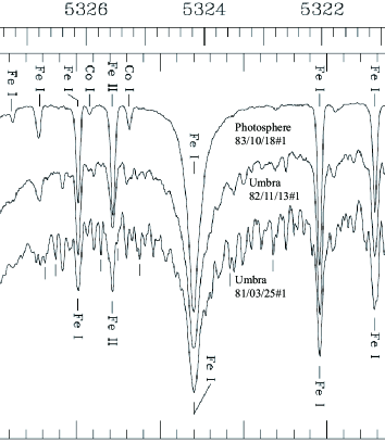
Figure 1: The spectra of FeI 5324.19 Å obtained from Kitt Peak observational results. From [16]

3.1 Formation of FeI$\lambda$5324.19Å Line in Photospheric Magnetic Field

The FeI$\lambda$5324.19Å line is a working line for the Huairou Vector Magnetograph (Solar Magnetic Field Telescope - SMFT) in National Astronomical Observatories of China (Ai & Hu, 1986) [15]. The FeI$\lambda$5324.19Å line in Figure 1 is a normal triplet in the magnetic field and the Lande factor g=1.5, the excitation potential of the low energy level of this line is 3.197eV. The equivalent width of the line is 0.33Å and the residual intensity at the core is 0.17 (Kurucz et al., 1984) [16]. This is a relatively wide line than other normal photospheric lines, such as the working lines used at the ground-based vector magnetographs, such as the FeI$\lambda$5250.2Å line (Lande factor g=3) used by the Video Vector Magnetograph at Marshall Space Flight Center (West & Hagyard， 1983) [17] and the FeI$\lambda$ 6301.5Å (Lande factor g=1.667) and FeI$\lambda$ 6302.5Å (Lande factor g=2.5) lines used by the Solar Polarimeter at Mees Solar Observatory (Ronan et al., (1987) [18]).

The bandpass of the birefringent filter of the Huairou Magnetograph with 3 sets KDP crystal modulators is about 0.15Å for the FeI$\lambda$5324.19Å line. The center wavelength of the filter can be shifted and is normally at -0.075Å from the line center of FeI$\lambda$5324.19Å for the measurement of longitudinal magnetic field and at the line center for the transverse one [15]. The theoretical calibration of Huairou Magnetograph was presented by Ai, Li & Zhang (1982) [7] and observational one by Wang, Ai, & Deng (1996) [19] and Su & Zhang (2004) [20].

3.2 Numerical Calculation of Radiative Transfer of Stokes Parameters

The theoretical analysis of Stokes parameters in the magnetic field is important for the diagnostic of the magnetic field in the solar atmosphere. Now, we firstly study the Stokes profiles of the FeI$\lambda$5324.19Å line under the VAL-C quiet Sun model atmosphere (Vernazza et al., 1981) [21] by the numerical calculation code of Ai, Li & Zhang (1982) [7] and fit the observed profile $I$ (Kurucz, et al., 1984 [16]) in the case of no magnetic field.

Figure 2 shows the Stokes parameters $I$, $Q$, $U$, $V$ of the FeI$\lambda$5324.19Å line, calculated with the VAL-C atmospheric model and a homogeneous magnetic field B from 500 to 4000 gauss, inclination of the field $\psi$=30^∘, azimuth $\varphi$=22.5^∘ and $\mu=1$. Figure 3 shows the comparison with the SW umbral model atmosphere [Stellmacher & Wiehr (1970), Stellmacher & Wiehr, (1975) [22, 23]]. Because we chose the azimuth angle of the field is 22.5^∘, the Stokes parameter $Q$ is equal to $U$ if the magneto-optical effect is ignored. Thus, the difference between Stokes parameters $Q$ and $U$ in Figure 2 and 3 provides the information of the Faraday rotation of the plane of polarization, in the real situation that that the magneto-optical effect cannot be ignored.

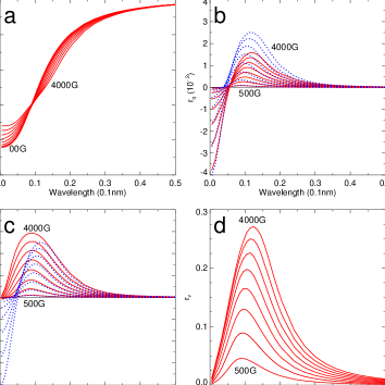
Figure 2: The Stokes parameters $r_{i},r_{q},r_{u}$, and $r_{v}$ (i.e. $I/I_{c}$, $Q/I_{c}$, $U/I_{c}$ and $V/I_{c}$) of the FeI$\lambda$5324.19Å line numerically calculated under the VAL-C model atmosphere (red solid lines) [21] with the inclination $\psi$=30^∘, azimuth $\varphi=22.5^{\circ}$, and $\mu=1$ for the strength from 500 to 4000 gauss with the interval of 500 gauss, but Stokes $I/I_{c}$ from 0 Gs. The blue dotted lines (in Figures b and c) mark $r_{q}$ and $r_{u}$ in the case that the magneto-optical effect has been ignored, respectively.

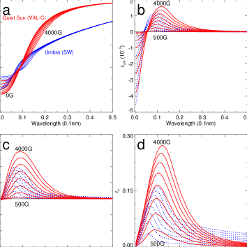
Figure 3: The Stokes parameters $r_{i},r_{q},r_{u}$, and $r_{v}$ (i.e. $I/I_{c}$, $Q/I_{c}$, $U/I_{c}$ and $V/I_{c}$) of the FeI$\lambda$5324.19Å line numerically calculated under the VAL-C model atmosphere (red solid lines) [21] with the inclination $\psi$=30^∘, azimuth $\varphi=22.5^{\circ}$, and $\mu=1$ for the strength from 500 to 4000 gauss with the interval of 500 gauss, but Stokes $I/I_{c}$ from 0 Gs, and the same case under the SW umbral model atmosphere (blue solid or dotted lines) [22, 23].

Figure 4 shows the the Stokes parameters $Q$, $U$ and $V$ calculated in Figure 3 in a almost equivalent form. It presents the curve clusters on the relationship between the strength of magnetic fields and the Stokes parameters $Q$, $U$ and $V$, and the “error azimuthal angles” of the transverse field inferred due to the magneto-optical effect with different wavelengths of the FeI$\lambda$5324.19Å in the quiet Sun (VAL-C) [21] and umbral [22, 23] model atmosphere. The solid lines in Figures 4a and 4b show Stokes $V/I_{c}$ in the wing of FeI$\lambda$5324.19Å at 0.075Å from the line center, while other solid lines in Figure 4c-f show $[(Q/I_{c})^{2}+(U/I_{c})^{2}]^{1/4}$ and “error azimuthal angles” of wavelength 0.005Å from the line center (i.e. almost at the line center).

Figure 4: The relationship amount the Stokes parameters $r_{v}$ and $(r^{2}_{qm}+r^{2}_{um})^{1/4}$ (i.e. $V/I_{c}$, $[(Q/I_{c})^{2}+(U/I_{c})^{2}]^{1/4})$ of the FeI$\lambda$5324.19Å line and magnetic strength in the wing from 0.005 to 0.185Å with the interval of 0.01Å in the quiet Sun (left) and umbral (right) model atmospheres. e-f) The “error azimuthal angles” of the transverse field inferred due to the magneto-optical effect. The others are the same with Figure 3. The $V/I_{c}$ relates to the longitudinal component of the field, while $Q/I_{c}$ and $U/I_{c}$ to the transverse one.

Figure 4 shows that the quiet Sun and sunspot atmosphere have different sensitivities of Stokes parameters of the spectral line. The ratio between the Stokes parameter $r_{v}$ (i.e. $V/I_{c}$) of the quiet Sun and sunspot umbra is about 1.8, and the linear approximation to Stokes $V$ can be used for relatively weak magnetic field only below 2000G for the quiet Sun and 1000G for the umbra, respectively. Similarly, the ratio between the Stokes parameter $(r^{2}_{qm}+r^{2}_{um})^{1/4}$ (i.e. $[(Q/I_{c})^{2}+(U/I_{c})^{2}]^{1/4}$) of the quiet Sun and sunspot umbra is about 1.5 normally and it changes with wavelengths. The linear approximation can be used for relative weak magnetic field only below 1000G for the quiet Sun and 600G for the umbra, respectively. These reflect the nonlinearity between the strength of magnetic fields and the measured polarized components of the spectral line.

It is presented from the observations [24] that the magneto-optical effect is a notable problem for the measurement of the transverse field with the FeI$\lambda$5324.19Å line. Although the magneto-optical effects have been neglected in some studies of the transverse magnetograms obtained by the Huairou magnetograph (Wang et al. 1992) [25], its influence is more obvious near the line center than in the far wing.

The magneto-optical effect is a notable problem for the diagnosis of magnetic field in solar active regions using magnetic sensitive lines by vector magnetographs (Landolfi and Landi Degl’Innocenti, 1982; West and Hagyard, 1983; Skumanich and Lites, 1987) [26, 17, 27], because it influences the determination of the azimuthal angle of the transverse magnetic field. The corresponding rotation of the azimuthal angles of polarized light related to the transverse components of the fields can be found in Figure 4.

Figure 5: The contribution functions $C_{i},C_{q},C_{u}$, and $C_{v}$ of Stokes parameters $I$, $Q$, $U$ and $V$ of the FeI$\lambda$5324.19Å line are numerically calculated under a VAL-C model atmosphere at the wavelengths $\triangle\lambda$=0.2 (cross), 0.155 (star), 0.075 (diamond), 0.035 (delta) and 0.005 (black) Å from the line center, with the magnetic field B=1000 Gauss, the inclination $\psi$=30^∘, azimuth $\varphi$=22.5^∘, and $\mu=1$.

The “error azimuthal angle” caused by the magneto-optical effect is defined as the difference between that of the magneto-optical effect and that of the non magneto-optical effect,

$$\bigtriangleup\varphi=0.5\left[\textrm{tg}^{-1}\left(\frac{U_{f}}{Q_{f}}\right)-\textrm{tg}^{-1}\left(\frac{U}{Q}\right)\right],$$ (15)

where the subscript $f$ marks that the Faraday rotation of the polarized spectral line has been considered. It is found that the “error azimuthal angle” of the transverse field obviously relates to the wavelength from the line center to the wing of the FeI$\lambda$5324.19Å line [24]. It is found that the “error azimuthal angle” of the transverse field is about 10^∘ near the line center and about 5^∘ at -0.15Å from the line center as the magnetic field is 1000 Gauss. Similar result for Stokes parameters $I$, $Q$, $U$ of the FeI$\lambda$5324.19Å line under the cool umbra model (Stellmacher & Wiehr, 1970) [22] can be found also. The “error azimuthal angle” of the transverse field is an order of about 20^∘ near the line center and about 10^∘ at -0.15Å. It is noticed that the maximum errors of the azimuthal angles of transverse components of the magnetic field can reach $\pm 20^{\circ}$ due to the magneto-optical effect in Figure 4.

Although we display some examples of the magneto-optical effects on the FeI$\lambda$5324.19Å line, but these provide a basic estimation on the order of “error azimuthal angles” for the measurement of the transverse magnetic field by the FeI$\lambda$5324.19Å line only. The “error azimuthal angle” relates to the inclination angle and intensity of the magnetic field from the calculations. The magneto-optical effects with the FeI$\lambda$5250.22Å line were calculated by Solanki (1993) [28] and also West & Hagyard (1983) [17]. It seems the different sensitivity of the magneto-optical effect relative to the FeI$\lambda$5324.19Å line. This is consistent with the result obtained by Landolfi & Landi Degl’Innocenti (1982) [26], i.e. the error in the azimuthal angle is larger for intermediate values of the Zeeman splitting (0.5$\leq$ $v_{H}$$\leq$2.5), if we keep in mind that the landé factor of the FeI$\lambda$5250.22Å line is 3.0 and that of the FeI$\lambda$5324.19Å line is 1.5, and the equivalent widths of these lines are different. We also notice that the calculated amplitude of the magneto-optical effect relates to the choices of the parameters of solar model atmospheres and the simplification of radiative transfer equations etc.

3.3 Formation Layers of Spectral Lines

It is important to know where in the solar atmosphere a given spectral line formed. This information is provided by the contribution function $C_{\textbf{ I}}$ defined by Stenflo (1994) [1]

$$\textbf{ I}(0)=\int_{0}^{\infty}C_{\textbf{ I}}(\tau_{c})d\tau_{c}=\int_{-\infty}^{\infty}C_{\textbf{ I}}(x)dx$$ (16)

for the Stokes vector $\textbf{ I}=(I,Q,U,V)$, where $C_{\textbf{ I}}(x)=(\textrm{ln}10)\tau_{c}C_{\textbf{ I}}(\tau_{c})$ and $x=\textrm{log}\tau_{c}$, $\tau_{c}$ is the continuum optical depth at 5000Å. It provides the contribution to the emergent Stokes parameters from the different layers of the solar atmosphere.

Now, we can define the equivalent source functions $S_{\textbf{ I}}^{\star}$ (Zhang, 1986)[9]

$$\begin{array}[]{c}\displaystyle S_{I}^{\star}=S-\frac{1}{\eta_{0}+\eta_{I}}[\eta_{Q}Q+\eta_{U}U+\eta_{V}V]{}{}{}{}{}{}\\ \displaystyle S_{Q}^{\star}=-\frac{1}{\eta_{0}+\eta_{I}}[(\eta_{Q}(I-S)+\rho_{V}U-\rho_{U}V)]{}\\ \displaystyle S_{U}^{\star}=-\frac{1}{\eta_{0}+\eta_{I}}[(\eta_{U}(I-S)-\rho_{V}Q+\rho_{Q}V)]{}\\ \displaystyle S_{V}^{\star}=-\frac{1}{\eta_{0}+\eta_{I}}[(\eta_{V}(I-S)+\rho_{U}Q-\rho_{Q}U)].\end{array}$$ (17)

Similar studies have been done by Jin (1981), Song et al. (1990), Qu et al. (1997) [29, 10, 12]. These represent formal radiative sources of Stokes parameters contributing to the emergent Stokes parameters at different layers of the solar atmosphere. The Unno-Rachkovsky equations of radiative transfer of polarized light can be written in a compact form

$$\mu\frac{d\textbf{ I}}{d\tau_{c}}=(\eta_{0}+\eta_{I})(\textbf{ I}-S_{\textbf{ I}}^{\star}).$$ (18)

It is the same as eq. (11.129) of [1] and $\mu$ is the cosine of the heliocenter angle. In the following, we analyze the line formation in the center of the solar disk, where $\mu=1$. We notice that the contribution functions in the far wings also bring some information of the continuum, while we also notice that the continuum does not significantly contribute to the Stokes parameter $V$ of the lines near the working wavelengths of the Huairou Magnetograph to influence the estimation on the formation layers of the Stokes parameters. The contribution function $C_{\textbf{ I}}$ is

$$C_{\textbf{ I}}(\tau_{ci})=\frac{1}{\mu}S_{\textbf{ I}}^{\star}\exp\left[-\frac{1}{\mu}\int_{0}^{\tau_{ci}}(\eta_{0}+\eta_{I})d\tau_{c}\right](\eta_{0}+\eta_{I}),$$ (19)

where $\tau_{ci}$ is the continuum optical depth at the $i$-th depth point. We can find that this contribution function obviously relates to the simple form of the radiative transfer equation (18) and can be used in the numerical calculation of the radiative transfer equations conveniently.

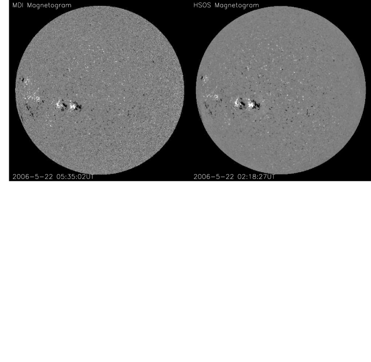
Figure 6: The comparison between the full disk longitudinal magnetograms observed form MDI of SOHO satellite (left) and vector magnetograph at Huairou (right) on 2006 May 22. From [31]

Figure 5 shows the formation depths of the FeI$\lambda$5324.19Å line in the solar VAL-C model atmosphere with different wavelengths within 0.005Å - 0.2Å from the line center. In the far wing $\bigtriangleup\lambda=0.2$Å, Stokes parameters $I$, $Q$, $U$, $V$ mainly form near the relative deep solar photosphere $\textrm{log}\tau_{5}\sim(-1,0)$, while near the line center $\bigtriangleup\lambda=0.005$Å Stokes parameters mainly form in the relative high photosphere $\textrm{log}\tau_{5}\sim(-3,-1)$, where $\tau_{5}$ means the optical depth of continuous spectrum at 5000Å.

The calculation provides that the Stokes parameters of the FeI$\lambda$5324.19Å line form below the solar temperature minimum region (about $\tau_{500\textrm{nm}}=10^{-4}\!\sim\!10^{-3}$) in the model atmosphere (Vernazza et al., 1976) [30]. This means that FeI$\lambda$5324.19Å is a typical photospheric line. The formation layer of the spectral lines in sunspots is different from that in the quiet Sun.

3.4 Measurements of Full Solar Disk Magnetic Field

Solar Magnetism and Activity Telescope (SMAT) is operated at Huairou Solar Observing Station, National astronomical Observatories of China started at 2003 (Zhang et al., 2007) [31]. A birefringent filter is centered at 5324.19Å for the measurement of vector magnetic field and the bandpass of the filter is 0.1Å. Figure 6 shows the comparison between both longitudinal magnetograms obtained by MDI of SOHO satellite and SMAT on 2006 May 22. It can be found the basic morphological correlation between both magnetograms. Some slight differences of both magnetograms are probably caused by the different seeing condition, observing noise, and also the data reducing methods.

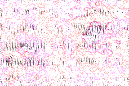
Figure 7: Local area of full disk vector magnetogram on 2006 April 28. The bars mark the transverse magnetic field. From [31]

A local area of the full disk vector magnetogram is shown in Figure 7. The strong transverse components of the field extend from the strong longitudinal field in the active regions. It is estimated that in this region the sensitivity of the longitudinal component of magnetic field is about or lesser than the order of 5 gauss and the transverse one is about 100 gauss in Figure 8.

Figure 9 shows the correlation between the vector magnetograms observed by SMFT and SMAT in an active region (Su & Zhang, 2007) [32]. The relationships of the longitudinal components, the transverse components, and the azimuthal angles of both vector magnetic fields are shown in the figure. It is found a relative high correlation between both vector magnetogams observed from SMFT and SMAT. The study on the spatial integration scanning spectra of filter magnetograph is also important for the calibration of the full-disk vector magnetic fields, which was made by Wang et al. (2010) [33].

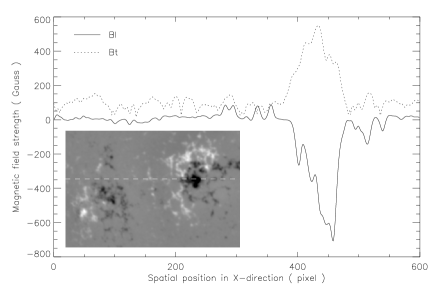
Figure 8: The intensity distribution of longitudinal and transverse magnetic field along the dashed beeline in the local area of full disk magnetogram on 2006 April 28 (bottom left), which vector magnetogram is shown in Figure 7. From [31]

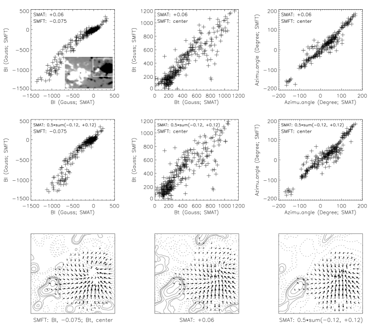
Figure 9: The relationship between the vector magnetograms observed by the SMFT and the SMAT in the region marked with the white box in the Stokes V image at the bottom-right corner of the first panel. The relationships of the longitudinal components, the transverse components and the azimuthal angles of the vector magnetic fields of both instruments are in the first two rows, the vector magnetograms in the last row. The wavelengths of both instruments are marked in each panel. In the scatter correlation plots, a 2.5 factor has been applied to the circularly polarized signal and a 3.0 factor to the linearly polarized signals of the SMAT. From [32]

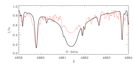
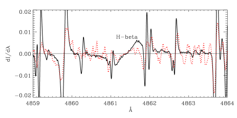
Figure 10: Left: H$\beta$ lines in the quiet Sun (solid line) and sunspot umbra (dotted line) observed by the National Solar Observatory of USA (L. Wallace, K. Hinkle, and W. C. Livingston, http://diglib.nso.edu/ftp.html). Right: $dI/d\lambda$ inferred by the corresponding H$\beta$ lines in above.

4 Formation of H$\beta$ Line in Solar Chromospheric Magnetic Field

It is believed that solar active phenomena often relate to the complex configurations of coronal and chromospheric magnetic fields. The observations of chromospheric magnetograms were made, such as, at the Crimean, Kitt Peak and Huairou Observatories (cf. Severny & Bumba (1958), Tsap (1971), Giovanelli (1980), Zhang et al. (1991) [34, 35, 36, 37]). The H$\beta$ line is a working line of SMFT at Huairou Solar Observing Station of National Astronomical Observatories of China for the measurements of chromospheric magnetic fields (Zhang & Ai, 1987) [38].

Table 1: Parameters of H_β line. $\gamma_{R}$ is the damping parameter, $gf$ is the oscillator strength and $gf_{w}$ is the normalized oscillator strength. [39, 38]

Transition	WL (Å)	$\gamma_{R}\times 10^{8}$	$gf$	$gf_{w}$
$2p_{1/2}-4d_{3/2}$	4861.279	6.5452	0.2436	0.2552
$2s_{1/2}-4p_{3/2}$	4861.287	0.8328	0.13702	0.1435
$2p_{1/2}-4s_{1/2}$	4861.289	6.3122	0.00609	0.0068
$2s_{1/2}-4p_{1/2}$	4861.298	0.8328	0.0685	0.0718
$2p_{3/2}-4d_{5/2}$	4861.362	6.5452	0.4385	0.45935
$2p_{3/2}-4d_{3/2}$	4861.365	6.5452	0.0487	0.0510
$2p_{3/2}-4s_{1/2}$	4861.375	6.3122	0.0122	0.01278

Figure 10 shows the solar H$\beta$ line profile and some photospheric lines overlap in the wing. The wavelength of the H$\beta$ line is 4861.34Å and its equivalent width is 4.2Å. The core of the line is formed at a height of about 1900 km (Allen, 1973) [40], while different formation heights of the H$\beta$ line were proposed by various authors. Its oscillator strength is 0.1193 and the residual intensity at the core is 0.128 (Grossmann-Doerth & Uexkull, 1975) [41]. It is normally believed that the Doppler broadening forms in the core of the H$\beta$ line, and resonance damping and Stark broadening in the wing. The H$\beta$ line is composed of 7 lines and all located within a width of nearly 0.1Å. We can use the formulae given by Bethe & Salpeter (1957) [39] to calculate individual component lines, the wavelength shift, the normalized oscillator strength and damping constant, which are shown in Table 1. In comparison with the results given by Allen (1973) [40] and Garcia & Mack(1965) [42], these available parameters showed slight difference in the mean wavelengths. When the magnetic field alone is present, the H$\beta$ line shows the anomalous Zeeman effect. In the solar atmosphere, both magnetic field and interatomic microscopic electric field are present, the wave functions of the hydrogen atom energy levels become degenerate, and different wave functions relate to complicated energy shifts.

4.1 Radiative Transfer of H$\beta$ Line

We study the formation of polarized light of the H$\beta$ Line with Eq. (7), Unno-Rachkovsky equations of polarized radiative transfer, in the solar atmospheric magnetic field. The source function $S_{\nu}$ in Eq. (6) for the line spectrum is departure from LTE with coefficients $b_{l}$ and $b_{u}$ in Eq. (5). We also assume the continuum to be LTE.

As a magnetic field is present, the broadening of the hydrogen line, such as H$\beta$, should be the joint effect of the magnetic field and the microscopic electric field distributed according to the Holtsmark statistics. It is assumed that the microscopic electric field is isotropic in the solar atmosphere, and their contribution to the polarization of the emergent light of the H$\beta$ line is negligible, thus the angular dependence and polarization properties of the $\pi$ and $\sigma$ components of the transitions of the H$\beta$ line can be obtained from the classical theory.

In comparison with formulae of the non-polarized hydrogen line proposed by Zelenka (1975) [43], Zhang & Ai (1987) [38] introduced the absorption coefficients of H$\beta$ line in the magnetic field atmosphere in the form

$$\eta_{p,l,r} = \eta_{0}{\sum_{i}f_{wi}H(a_{i},v_{i}(\triangle m))\int_{0}^{\beta_{l}}W(\beta,r_{0}}/D)d\beta$$

$$+ \frac{1}{4\pi}\eta_{0}{\sum_{j}f_{wj}\int_{0}^{2\pi}\int_{0}^{\pi}\int_{\beta_{l}}^{\infty}H\left(S(a_{j},\lambda)\right)}$$

$$W(\beta,r_{0}/D)d\beta\sin\theta d\theta d\chi,$$

and

$$\rho_{p,l,r} = 2\eta_{0}{\sum_{i}f_{wi}F(a_{i},v_{i}(\triangle m))\int_{0}^{\beta_{l}}W(\beta,r_{0}/D)d\beta}$$

$$+ \frac{1}{2\pi}\eta_{0}{\sum_{j}f_{wj}\int_{0}^{2\pi}\int_{0}^{\pi}\int_{\beta_{l}}^{\infty}F\left(S(a_{j},\lambda)\right)}$$

$$W(\beta,r_{0}/D)d\beta\sin\theta d\theta d\chi,$$

where $S(a_{j},\lambda)=\left(a_{j},\frac{\triangle\lambda-\triangle\lambda_{j}(\theta,\chi,\beta,\triangle m)}{\triangle\lambda_{D}}\right)$ and $f_{wi}$ and $f_{wj}$ are normalized oscillator strengths of polarized subcomponents of the H$\beta$ line. $W(\beta,r_{0}/D)$ is the Holtsmark distribution function of the microscopic electric field. $\beta_{l}$ is a criterion to measure the relative size of the shift caused by the electric field, relative to the fine structure of the hydrogen line. If $\beta_{l}$ is very large, then the effect of the electric field can be negligible.

For H$\beta$ line, we can choose $\beta_{l}=0.1189/F_{0}=9.512\times 10^{12}N_{e}^{2/3}$. Then, the second terms on the right of formulae (4.1) and (4.1) for the lower solar atmosphere are the main terms and the effect of the interatomic electric field is all important. As we go up in the chromosphere, the density of charged ions falls and the first term becomes more and more important.

The first terms in the formulae (4.1) and (4.1) reflect the contribution under the weak microscopic electric field, thus the approximation of Zeeman splitting is suitable. There $v_{i}(\triangle m=1)$, $v_{i}(\triangle m=0)$ and $v_{i}(\triangle m=\!-1)$ connected with Zeeman splitting are following, for $k=1,2,3$, $\displaystyle v_{i}(\triangle m=2-k)=v-v_{m}^{(k)},$ and

$$v_{m}^{(k)}=\frac{e\lambda^{2}H}{4\pi m_{e}^{2}\triangle\lambda_{D}}[(G-G^{\prime})M-G^{\prime}(2-k)].$$ (22)

Here, $M$ is the magnetic quantum number of the lower energy level, $G$ and $G^{\prime}$ are the landé factors for the lower and upper levels. $f_{wi}$ is the normalized oscillator strengths of the Zeeman sub-components of the H$\beta$ line.

While the second terms in the formulae (4.1) and (4.1) reflect the common contribution of the magnetic field and strong microscopic electric field to the line broadening. $\triangle\lambda_{j}$ is the shift of the polarized $j$-component of the spectral line caused by the magnetic and strong statistical electric field. $f_{wj}$ is the normalized oscillator strength of the polarized sub-components of the H$\beta$ line in the magnetic and microscopic electric field.

The damping parameter of $i$-th component of the line is $\displaystyle a_{i}=\frac{\gamma_{i}\lambda_{0}^{2}}{4\pi c\triangle\lambda_{D}},$ where $\displaystyle\gamma_{i}=(\gamma_{\textrm{radiation}}+\gamma_{\textrm{resonance}}+\gamma_{\textrm{electron}})_{i}.$

Now, a hydrogen atom and a perturbing, charged particle have been considered in the external magnetic and electric field. The hamiltonian of the hydrogen atom can be written

$$\hat{H}=\hat{H}_{0}+\hat{V}_{H}+\hat{V}_{F},$$ (23)

where the first term on the right is the unperturbed hamiltonian, the second and third terms represent the perturbation of the magnetic field and electric field, respectively. The perturbation equation is

$$(\hat{H}_{0}+\hat{V}_{H}+\hat{V}_{F})\mid\psi\rangle=(E_{0}+E^{\prime})\mid\psi\rangle,$$ (24)

where $E_{0}$ and $E^{\prime}$ are the energy eigen value and perturbation, respectively. One can calculate the shifts $\triangle\lambda_{j}$ of the sub-components of the spectral line by means of Eq. (24). Normally, the general solution of the eigenvalue problem for the hydrogen lines does not depend on the direction of the magnetic field and microscopic electric field. The choice of the coordinate system for the calculation of the Hermitian matrix of the perturbing Hamiltonian was made by Casini & Landi Degl’Innocent (1993) [44].

4.2 Numerical Calculation of H$\beta$ Line

For analyzing the general properties on the formation of the H$\beta$ line, we used the VAL mean quiet chromospheric model $C$ (Vernazza et al., 1981) [21] and relevant non-LTE departure coefficients. We assumed that, when the degeneracy of energy levels disappears under the action of the magnetic field and microscopic electric field, each magneton energy level keeps its original departure coefficient. It is only an approximation. The emergent Stokes profiles of H$\beta$ line are shown in Figure 11. The calculation results show that the influence of the magneto-optical effect for Stokes parameter $V$ is insignificant, but that for Stokes parameters $Q$ and $U$ in the H$\beta$ line center is significant, for example the error angle of the transverse field is about 7^∘. Even though， this means that the influence of the magneto-optical effect for H$\beta$ line is weak than that of the photospheric lines, such as FeI$\lambda$5324.19Å line.

Figure 11: Profiles of Stokes parameters $r_{i},r_{q},r_{u}$, and $r_{v}$ (i.e. $I/I_{c}$, $Q/I_{c}$, $U/I_{c}$ and $V/I_{c}$) of the H$\beta$ line calculated for the VAL model atmosphere, a homogeneous magnetic field intensity 1000-3000 gauss of inclination $\psi$=30^∘, azimuth $\varphi$=22.5^∘ and $\mu=1$. $I_{c}$ is the continuum.

By comparing the calculated signals of H$\beta$ line for the measurement of chromospheric magnetic field in Figure 11 with the photospheric one with the FeI$\lambda$5324.19Å line in Figure 3, it is found that their ratio on the peak values of Stokes $V$ in the wing of both lines is about a order of 0.18 (0.04/0.22), while the that of Stokes $Q$ is 0.06 (0.0007/0.012) for 3000 gauss magnetic field. Because the the core of the H$\beta$ line is too flat, this is consistent with the calculated result of the weak signals of Stokes $Q$ and $U$ about a order of $10^{-4}$ in Figure 11. This implies that the longitudinal components of the H$\beta$ chromospheric magnetic field are detectable, while the challenge with the high accuracy diagnostic occur in the measurements of the transverse components of the chromospheric fields.

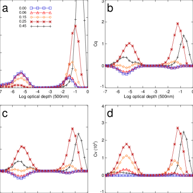
Figure 12: Contribution functions $C_{i},C_{q},C_{u}$, and $C_{v}$ of Stokes parameters $I$, $Q$, $U$ and $V$ of the numerical solution of H$\beta\lambda$4861.34Å line calculated for the VAL model atmosphere at the wavelengths $\triangle\lambda$=0.45 (cross), 0.25 (star), 0.15 (diamond), 0.06 (delta) and 0.0 (black) Å from the H$\beta$ line center. B=1000 gauss, $\psi$=30^∘, azimuth $\varphi$=22.5^∘ and $\mu=1$. $\tau_{c}$ is continuum optical depth at 5000Å. The horizontal coordinate is in the logarithmic scale.

The contribution functions of Stokes parameters of the H$\beta$ line calculated with the VAL model atmosphere [21] are shown in Figure 12. We can see that in our calculation the emergent Stokes parameters at H$\beta$ line center almost form in the higher atmosphere (1500-1600 km), but that in the wing, for example, at -0.45Å away from the H$\beta$ line center the emergent Stokes parameters reflects the information of the photospheric field (300 km). The formation height of the Balmer lines in the solar atmosphere excluding the magnetic field was analyzed also by several authors cf. Gibson (1973) [45]. From the calculated results, we can see that the formation heights of Stokes parameters $Q$, $U$ and $V$ are almost the same to $I$.

It is needed to point out that real formation layers of Stokes parameters of the H$\beta$ line are more complex than theoretical cases. Numerical results of the equations of radiative transfer depend on the selection of atmospheric models and parameters of spectral lines. For example, the formation height near the line center obviously depends on the selection of the value of the absorption coefficient of the line; and in the wing of the line that also depends on the amplitude of the line broadening. The formation layers of different kind of structures observed in the H$\beta$ images in the solar atmosphere may be different, such as sunspot umbrae, penumbrae and dark filaments, even though these features are observed at the same wavelength in the wing of the chromospheric line. However, the computation of the formation layers of the line provides us a reference to estimate the possible spatial distribution of the detected magnetic field.

4.3 Possibility of Reversal Features in H$\beta$ Chromospheric Magnetograms

Figure 13 shows active region NOAA6619 on May 10 1991. The 180^∘ ambiguity of transverse components of the vector magnetic field probably is an obstinate question in the measurements of magnetic fields with the polarized spectral lines. In Figure 13, the 180^∘ ambiguity of transverse components of the photospheric vector magnetic field has been resolved under the assumption of the minimizing the vertical gradient of the magnetic pressure and minimizing some approximation to the field’s divergence etc. cf. also Metcalf et al. (2006) [46].

It is found the twisted photospheric magnetic field formed in the compacted delta active region, and the vector magnetic field extends form photosphere into the chromosphere in the fibril-like features in the active region. The chromospheric reversal signal structure in the center of sunspot relative to positive polarity in the photosphere can be found. The similar results have been presented, such as, by Chen et al. (1989), Zhang et al. (1991), Almeida (1997), Zhang (2006) [47, 37, 48, 49].

Due to the disturbance of the photospheric blended lines, such as FeI$\lambda$4860.98Å, nearby the H$\beta$ line center, the reversal signal in the chromospheric magnetograms relative to the photospheric ones occurs in the sunspot umbrae in Figure 13. It is the same with the reversal of Stokes $V$ nearby the line center in Figure 10. In the approximation of the week magnetic field (Eqs. (12) and (13)), the sensitivity of longitudinal magnetic field is proportional to the variation of the line profile $V\!\sim dI/d\lambda$ with the wavelength (Stenflo et al., 1984) [50].

Figure 14 shows the statistical distribution of Stokes parameter $V$ at the different wavelengths in the blue wing from the H$\beta$ line center [51] at the umbra of a solar active region. It is based on a series of the longitudinal magnetograms observed at Huairou Solar Observing Station. It confirms the disturbance of FeI 4860.98Å in the measurements of chromospheric magnetic fields.

It is noticed that in the quiet, plage regions, and even penumbrae, the influence of the photospheric blended FeI$\lambda$4860.98Å line is generally insignificant. As regards the H$\beta$ chromospheric magnetograms, we can select the working wavelength between -0.20 and -0.24Å from the line core of H$\beta$ to avoid the wavelengths of the photospheric blended lines in the wing of H$\beta$. A similar evidence on the disturbance of blended lines in the wing of H$\alpha$ is presented by Hanaoka (2005) [52].

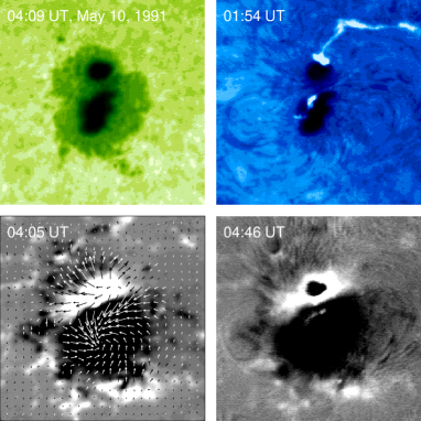
Figure 13: Active region NOAA 6619 on May 10 1991. Top left: Photospheric filtergram. Bottom left: Photospheric vector magnetogram. Top right: H$\beta$ filtergram. Bottom right: H$\beta$ longitudinal magnetogram. White (black) is positive (negative) polarity in the magnetograms. The size of each figure is $2.^{\prime}8\times 2.^{\prime}8$.

Figure 14: Statistical distribution of Stokes parameter $V$ in the blue wing of H$\beta$ line in the umbrae of a solar active region. From [51]

A comparison between photospheric and chromospheric H$\beta$ magnetograms in the quiet-Sun was provided by Zhang & Zhang(2000) [53], who found the similar patterns of the magnetic elements in the photosphere and chromosphere. It probably brings a message that the magnetic field extends in the form of the fibril-like configuration in the quiet Sun. The fibril-like magnetic features can also be found around the sunspots in the chromospheric magnetogram of Figure 13.

From the presentation above, it is found the complexity and difficulty on the diagnostic of chromospheric magnetic fields relative to the photospheric ones.

5 Magnetic fields in solar active regions

5.1 Non-potentiality of magnetic fields from observations

Figure 15 shows the vector magnetogram and Dopplergram of active region NOAA5395 on March 11 1989, observed at the Huairou Solar Observing Station of the National Astronomical Observatories of China.

Ai et al. (1991) [54] indicated that the flares in active region NOAA5395 tend to occur on the redshift side of the inversion lines of the H$\beta$ Doppler velocity fields observed half to two hours before. A similar case can be confirmed in Figure 15, although in this Dopplergram the disturbance from the flare sites cannot be neglected, due to the almost same observing times between this Dopplergram and the flare.

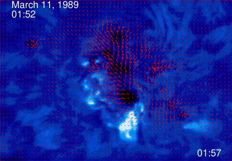
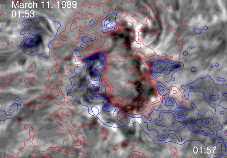
Figure 15: Left: A resolved the 180^∘-ambiguity of transverse components of photospheric vector magnetic field in the active region (NOAA 5395) at 01:57 UT on March 11, 1989, which is overlaid by a H$\beta$ filtergram at 01:52 UT. The arrows mark the directions of transverse magnetic field. Right: A corresponding H$\beta$ Dopplergram of the active region at 01:53 UT with longitudinal components of magnetic field. The red (blue) contours correspond to positive (negative) fields of ${\pm}$50, 200, 500, 1000, 1800, 3000 gauss. The white (black) indicates up-(down-)ward follow. The size of magnetogram is $5.^{\prime}23\times 3.^{\prime}63$. The north is top and the east is at left.

Some evidence in this powerful flare-producing region also can be found (Zhang (1995) [55]): 1) The twisted transverse magnetic field occurred in bay-like magnetic main poles of opposite polarity in the active region. The main poles of opposite polarity in this region moved apart at a speed of about 0.15km/s. 2) The newly-sheared vector magnetic structures formed near the magnetic neutral line between the collided magnetic main poles of opposite polarity. With the emergence of new magnetic flux, the change of sheared angles of the horizontal magnetic field between the magnetic main poles of opposite polarity is insignificant in comparison with daily vector magnetograms, but the distribution of the intensity of the vertical current inferred from the horizontal magnetic field evolved only gradually. 3) The flare sites occurred near the magnetic islands and bays of opposite polarity and were associated with the change of the vector magnetic field. Although some of the flare sites are located near the peak areas of the vertical electrical current density, their corresponding relationship is insignificant.

5.2 Magnetic Shear and Gradient

The magnetic shear is an important parameter to measure the non-potentiality of magnetic field in solar active regions (cf. Severny, (1958), Hagyard et al. (1984), Chen et al. (1989), Chen et al. (1994), Lü, Wang, & Wang (1993), Schmieder et al. (1994), Wang et al. (1994), Zhang et al. (1994), Li et al. (2000), Wang et al. (2000) [56, 57, 47, 58, 59, 60, 61, 62, 63, 64]), while the non-potential field can also be measured from the strong magnetic gradient of active regions, which is strongly correlated with active region flare-CME productivity (cf. Severny (1958), Falconer (2001) [56, 65]. The change of vector magnetic fields during the solar flares was observationally presented, such as, by Chen et al. (1989) [47].

For analyzing the relationship between the non-potential magnetic field and electric current in solar active regions, the photospheric vector magnetograms, after the resolution of 180^∘-ambiguity of transverse components of field, in the $\delta$ active region NOAA 6659 in June 1991 are shown in Figure 16, which observed at Huairou Solar Observing Station. A series of powerful flares occurred in this active region as studied by Zhang (1996) [66]. It is found that the high shear of transverse magnetic field and gradient of longitudinal magnetic field formed near the magnetic neutral line of the active region, where the transverse magnetic field rotated counterclockwise around the magnetic main pole of negative polarity.

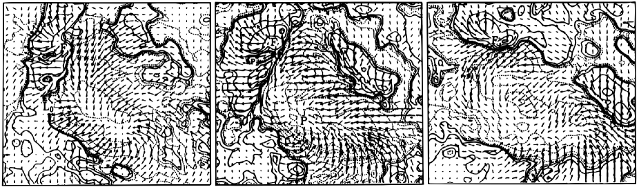
Figure 16: Ambiguity-resolved vector magnetograms at 0050 UT on 1991 June 6, at 0353 UT on 1991 June 9, and at 0438 UT on 1991 June 12 (from left to right) transformed from the image plane to heliographic coordinates. The contours indicate the longitudinal magnetic field distribution, $\pm$20, 160, 640, 1280, 1920, 2240, 2560, and 2880 G. From [66]

The shear angle can be weighted by the transverse magnetic field cf. Hagyard et al. (1984) [57]

$$\theta_{T}=B_{oh}\cdot\cos^{-1}\left(\frac{\textbf{ B}_{oh}\cdot\textbf{ B}_{ph}}{B_{oh}B_{ph}}\right),$$ (25)

where $B_{oh}$ and $B_{ph}$ are the observed transverse field and that calculated from the magnetic charges in the approximation of potential field. The amplitude of the shear angle in eq. (25) reflects the non-potentiality of the active region.

The horizontal gradient of the photospheric longitudinal magnetic field in active regions can be inferred from (cf. Leka & Barnes (2003) [67])

$$|\bigtriangledown(B_{z})|=\sqrt{\left(\frac{\partial B_{z}}{\partial x}\right)^{2}+\left(\frac{\partial B_{z}}{\partial y}\right)^{2}}.$$ (26)

The main contribution of magnetic shear in the active regions comes from the deviation of the transverse field from the potential field inferred by magnetic charges in the photosphere, while the magnetic gradient comes from the non-uniformity of the longitudinal field.

As one knows the non-potential magnetic field formed in solar active regions means the existence of electric current (cf. Moreton & Severny, (1968) [68]). The relationship between the magnetic field and electric current is

$$\textbf{ J}=\frac{1}{\mu_{0}}\bigtriangledown\times\textbf{ B},$$ (27)

where J is in units of $\textrm{Am}^{-2}$ and $\mu_{0}=4\pi\times 10^{-3}\textrm{GmA}^{-1}$ is the permeability in free space.

Figure 17: (a) Photospheric vector magnetic field in the active region (NOAA 6659) at 05:29 UT on June 9, 1991. The white (black) shows the positive (negative) polarity and arrows mark the transverse field. The corresponding vertical electric current (b) inferred by the term of the magnetic chirality of the magnetic field and (c) by the term of the magnetic gradient and shear term in Eq. (29). The solid (dashed) contours correspond to the upward (downward) flows of vertical currents of ${\pm}$ 0.002, 0.008, 0.02, 0.04, 0.075, 0.12 $\textrm{Am}^{-2}$. The size of view is $2.^{\prime}72\times 2.^{\prime}72$.

As letting $\textbf{ B}=B\textbf{ b}$ and b is the unit vector along the direction of magnetic field, the current may be written in the form [69]

$$\textbf{ J}=\frac{B}{\mu_{0}}\bigtriangledown\times\textbf{ b}+\frac{1}{\mu_{0}}(\bigtriangledown B)\times\textbf{ b}.$$ (28)

It is found that the electric current in solar active regions relates to the properties of chirality and gradient of magnetic field. The first term in eq. (28) connects with the twist of unit magnetic lines of force and intensity of the field. The second term in eq. (28) connects with the heterogeneity and orientation of magnetic field.

The vertical electric current can be written according to Eq. (28)

$$J_{z}=\frac{B}{\mu_{0}}\left(\frac{\partial{b}_{y}}{\partial x}-\frac{\partial{b}_{x}}{\partial y}\right)+\frac{1}{\mu_{0}}\left({b}_{y}\frac{\partial B}{\partial x}-{b}_{x}\frac{\partial B}{\partial y}\right),$$ (29)

where ${b}_{x}={{B}_{x}}/{B}$ and ${b}_{y}={{B}_{y}}/{B}.$ The distribution of the two current components in active region NOAA6659 is shown in Figure 17.

Similar studies by means the two current components of active regions were taken, such as, on the resolution of the azimuthal ambiguity of vector magnetograms of solar active regions (Georgoulis et al. (2004) [70]), and the non-potentiality of solar active regions (Vemareddy (2017) [71]).

5.3 Free Energy Contributed from Non-potential magnetic fields

Now we analyze the free magnetic energy contributed from different components of magnetic fields (which is similar to Priest (2014) [72], p117)

$$W_{o} = \frac{1}{2\mu_{0}}\int B_{o}^{2}dV=\frac{1}{2\mu_{0}}\int(B_{n}^{2}+2\textbf{ B}_{n}\cdot\textbf{ B}_{p}+B_{p}^{2})dV$$ (30)

$$= \frac{1}{2\mu_{0}}\int(B_{n}^{2}+2\textbf{ B}_{n}\cdot\textbf{ B}_{p})dV+W_{p},$$

where $W_{o}$ is the observed magnetic energy, $W_{p}$ is the potential magnetic energy, $B_{o}$ is the observed magnetic field, $B_{n}$ is the non-potential component of magnetic field and $B_{p}$ is the potential component of magnetic field, respectively.

As we set $\textbf{ B}_{p}=\nabla\psi$, it is fund the free energy

$$W_{f}=W_{o}-W_{p}=\frac{1}{2\mu_{0}}\int B_{n}^{2}dV+\frac{1}{\mu_{0}}\oint_{S}\psi\textbf{ B}_{n}\cdot d\textbf{ s}.$$

If the vertical component $B_{ns}=0$ in the surface $S$ of the close volume, it is found

$$W_{f}=\frac{1}{2\mu_{0}}\int B_{n}^{2}dV.$$ (31)

While Zhang (2016) [73] noticed that the contribution of the parameter $\frac{1}{\mu_{0}}\textbf{ B}_{n}\cdot\textbf{ B}_{p}$ in the solar surface cannot be neglected normally in the evolution of the flare-productive regions. This probably means the non-potential components of magnetic fields extend from the subatmosphere and bring the free energy into the atmosphere.

Figure 18: Butterfly diagram of the electric current helicity. The mean density of the current helicity of active regions is marked by size of the circles for grades: 0, 1, 3, 5, 7 ($10^{-3}\textrm{G}^{2}\textrm{m}^{-1}$). The filled and hollow circles mark the negative and positive sign of helicity. The dash-dotted line marks the average value of current helicity and the dashed line marks the average value of the imbalance of current helicity after the data smooth. From [81]

6 Distribution of Magnetic Helicity with Solar Active Cycles

According to the formula of current helicity density (Bao & Zhang, 1998) [74], the vertical component of current helicity density in the photospheric lyaer can be inferred by photospheric vector magnetograms

$$h_{\bot c}=(\textbf{ B}\cdot\bigtriangledown\times\textbf{ B})_{\bot}\sim\alpha B^{2},$$ (32)

where $\alpha=\textbf{ b}\cdot\bigtriangledown\times\textbf{ b}$.

In addition to the solar flare activities with helicity, such as, Bao et al. (1999), Zhang et al. (2008), Yang et al. (2012) [75, 76, 77], it is found that the mean magnetic helicity density in the solar active regions tends to show negative signs in the northern hemisphere and positive ones in the southern hemisphere (Seehafer (1990), Pevtsov, Canfield, & Metcalf (1995), Abramenko et al. (1996), Bao & Zhang(1998), Zhang & Bao (1998), Hagino & Sakurai (2004), Hao & Zhang (2011) [78, 79, 80, 74, 81, 82, 83] ). Figure 18 shows the distribution of mean current helicity density of active regions in 1988 - 1997 inferred from vector magnetograms observed at Huairou Solar Observing Station. Moreover, the reversal sign of helicity in these statistical work has also attracted much attention [84]. The change of magnetic helicity with solar cycles, such as helicity butterfly diagram, also bring some new thoughts on the generations of magnetic fields with the dynamo process in the subatmosphere (such as, Kleeorin et al. (2003), Zhang et al. (2012), Pipin et al. (2013) [85, 86, 87]).

7 The question on accuracy of measured vector magnetic fields

In addition to some fundamental achievements on discovering some important properties of solar magnetic activities, it is also needed to notice that the magnetic fields and relevant parameters, such as helicity etc., observed with different instruments not only have shown the basic same tendency, but also with some differences [25, 88, 89, 90]. As a sample, the discrepancies on the statistical distribution of the current helicity parameters $h_{c}$ and $\alpha$ of solar active regions obtained by different solar vector magnetographs at Huairou in China and Mitaka in Japan can be found by Xu et al. (2016) [90] in Figure 19.

Figure 19: Correlations in (a) $h_{\rm c}$ and (b) $\alpha_{\rm av}$ obtained from SMFT (Huairou) and SFT (Mitaka) data. The values of correlation coefficients (CC) are shown on the panels. From [90]

This relates to a basic question on the accuracy for the measurements of the solar magnetic fields by means of solar vector magnetographs and the corresponding observing theories of solar magnetic fields. Some restrictions on the calibration of magnetic field from Stokes parameters have been presented due the nonlinearity and simplicity in the above calculation of the radiative transfer equations of the spectral lines in solar magnetic atmosphere. It means that there are still some questions on the theories of the solar observations relative to the diagnostic with the radiative transfer of spectral lines, even if some problems of solar instrumental techniques have been ignored.

8 Discussions for some new challenges on measurements of solar magnetic fields

We have introduced the fundamental background of the radiative transfer process of the magnetic sensitive lines in the solar magnetic atmosphere, and corresponding analysis of solar vector magnetograms based on the study at Huairou Solar Observing Station of National Astronomical Observatories, Chinese Academy of Sciences.

As a series of vector magnetograms have been observed and some relevant interesting results have been presented from these observations, we should notice that the meticulous fine analysis based on the relative complex calculated from observed magnetograms probably is still needed, even if some results probably are more interesting, such as the meticulous configuration and variation of the magnetic shear, free energy density, electric current and helicity in the solar active regions. We probably also need to keep in mind that the quantitative analysis of solar magnetic field from observed magnetograms contains some intrinsic difficulties.

This means that there are still some basic questions on the measurements of solar magnetic fields need to be carefully analyzed. Some of them have been presented in the following:

• Radiative transfer of magnetic sensitive lines:

  We have presented the radiative transfer equations of magneticlly sensitive lines under the different approximations， whether ignoring the scattering or the assumption of thermodynamic equilibrium, such as the numerical and analytical forms (in subsec. LABEL:se:rtsp), which bring some ambiguity for the accurate results.

  The analytical solution has normally been used to inverse the photospheric vector magnetic fields. This means that the varieties of solar atmosphere models, such as the sunspot, facula and quiet Sun, have been ignored. From the calculated results, we can find the different magnetic sensitivities of polarized spectral lines for the different kinds of solar atmospheres, such as the quiet Sun and sunspots in Figure 4. It is also noticed that the different sensitivity for the measurements of the longitudinal and transverse components of magnetic field can be easily found from Eqs. (10), i.e. the longitudinal and transverse fields relate to the first and second order derivative of the profiles of spectral lines, respectively. In the condition Eqs. (13) and (14) of the approximation of the weak fields, the influence of magneto-optical effects has been neglected for the transverse components of the magnetic fields obviously. We can find that these provide the constraint condition on the observations of solar magnetic fields by different approximate methods or situations.

• Solar model atmosphere:

  We have presented the observations of photospheric vector magnetic fields with the FeI$\lambda$5324.19Å line and chromospheric magnetic fields with the H$\beta$$\lambda$4861.34Å line based on the analysis of the radiative transfer equations for polarized radiation by Unno (1956) [4] and Rachkovsky (1962a, b) [5, 6] under the assumption of local thermodynamic equilibrium or their extension to non-local thermodynamic equilibrium at Huairou Solar Observing Station.

  Even if the numerical calculation can be used in the analysis of the radiative transfer equations (7) of Stokes parameters and provides some important information on the formation of polarized spectral lines in the different atmosphere models, it still rarely has been used in the real inversion of the magnetic field, due to some difficulty and arbitrariness in the accurate selections of inputed atomic and solar parameters.

  It is noticed that the different formation heights of magnetic sensitive lines occur in the quiet Sun and sunspots, such as the Wilson effect of sunspots, due to the the transparency of sunspots, for the measurements of photospheric magnetic field, and the different heights for different chromospheric features, such as the prominence, fibrils and plages etc. This means that the observed magentograms probably does not always provide the information of magnetic fields at the same height in the solar atmosphere, even if at the similar optical depths of the working spectral lines.

  A notable question is the detection of the configuration of magnetic fields in the solar eruptive process, cf. Chen et al. (1989) [47]. Some study with Stokes parameters of spectral lines can be found (Hong et al.(2018) [91]). Due to the distortion of the spectral lines with the variation of solar atmosphere in the solar eruptive process [3], the analysis of relevant Stokes parameters of the spectral lines is a notable topic.

• Measurements of magnetic fields in the corona:

  The Hanle effect is a reduction in the polarization of light when the atoms emitting the light are subject to a magnetic field in a particular direction, and when they have themselves been excited by polarized light. The Hanle effects with polarized light in the corona is notable question for the measurements of the coronal magnetic fields, cf. Liu & Lin (2008), Qu et al. (2009), Li et al. (2017) [92, 93, 94].

  The analysis of the polarized lights due to the Hanle effect for the diagnostic of the coronal magnetic field is still a challenging topic [1].

• 180^∘ ambiguity on the determination of transverse magnetic fields:

  The resolution of the 180^∘ ambiguity of transverse fields is a difficult question due to the property of polarized light with Zeeman effects.

  Several basic assumptions and approaches have been used to resolve the 180° ambiguity of transverse components of magnetic fields, such as comparing the observed field to a reference field or direction, minimizing the vertical gradient of the magnetic pressure, minimizing the vertical current density, minimizing some approximation to the total current density, and minimizing some approximation to the field’s divergence (Metcalf et al. (2006) [46], Georgoulis (2012) [95]). Which of these treatments is prioritized is still debatable or questionable.

  The projection of vector magnetic fields from solar disk to the heliospheric coordinates relates the transform of the different components of magnetic field [96], such as in Figure 16, while the different Stokes parameters relate to different sensitivities and noise levels (cf. Eqs. (10)). This leads to the inconsistency in the transformation of different components of magnetic fields. It also causes degradation in spatial resolution of the vector magnetic fields after the inevitable smoothing fields from the image plane to heliographic coordinates in Figure 16.

• Diagnostics of electric fields in solar atmosphere:

  The Stark effect is notable in the broadened wings of hydrogen and helium lines. It has been used in the analysis of the radiative transfer of H$\beta$ line for the measurements of magnetic fields at Huairou Solar Observing Station, see Eqs. (4.1) and (4.1).

  The Stark effect is the shifting and splitting of spectral lines of atoms and molecules due to the presence of an external electric field. Normally, the isotropic plasma is statistically electrically neutral, due to the Debye effect. The electric fields in the solar flares were presented by Zhang & Smartt (1986) [97] based on the spectral analysis of the linear and quadratic components of the Stark broadening.

  A dynamic and quantitative depiction of the induction electric field $\textbf{E}=\textbf{u}\times\textbf{B}$ on the changes of the active regions was described by Liu et al. (2008) [98], where u is the velocity of the footpoint motion of the magnetic field lines and B is the magnetic field. E represents the dynamic evolution of the velocity field and the magnetic field, shows the sweeping motions of magnetic footpoints, exhibits the buildup process of current, and relates to the changes in nonpotentiality of the active region in the photosphere.

  The measurements of the polarized light due to the Stark effect (or electric fields) in the anisotropic plasma is also a challenging topic.

• Horizontal component of electric current and corresponding helicity:

  The observations of chromospheric magnetic field are important for diagnosing the spatial configuration of magnetic lines of force as compared with the photospheric one, while the disturbance of photospheric blended lines in the wing of H$\beta$ line also bothers the detection of the magnetic field in the high solar atmosphere in Figure 14. The lower sensitivity of Stokes $Q$ and $U$ of the H$\beta$ line cripples the observations of the transverse components of chromospheric magnetic fields.

  The electric current helicity density $h_{c}=\langle\varepsilon_{ijk}b_{i}{\partial b_{k}/\partial x_{j}}\rangle$ contains six terms, where $b_{i}$ are components of the magnetic field. Due to the observational limitations, only four of the above six terms can be inferred from solar photospheric vector magnetograms. By comparing the results for simulation, Xu et al. (2015) [99] distinguished the statistical difference of above six terms for isotropic and anisotropic cases. This means that the electric current and magnetic (current) helicity inferred from the photospheric vector magnetograms do not contain the completeness in theoretical sense.

• The limited spatial resolution for the measurements of magnetic fields:

  It is normally believed that the mean free path of photons emerging from the solar photosphere and chromosphere is about 100 km (Zuccarello (2012), Judge et al. (2015) [100, 101]). This relates to the detection of the magnetic flux tules in the solar atmosphere and their possible distribution.

• Influence of the Doppler motion for the measurements of solar magnetic fields:

  The influence for the measurements of magnetic fields from the Doppler velocity field due to the solar rotation was discussed (such as by Wang, Ai, & Deng (1996) [19]), and some for Doppler measurements of the velocity field in the solar photosphere and implications for helioseismology can be found (Rajaguru et al. (2006) [102]). However, the influence on the accuracy of the magnetic field measurement for the moving objects in the solar atmosphere is still a subject worth exploring.

Based on the above discussions, we can find that the diagnostic of solar magnetic fields in the solar atmosphere still is a fundamental topic. Although we have made some achievements on the analysis of solar vector magnetic fields based on the theory of the radiative transfer of spectral lines from observations, the quantitative study and the corresponding assessment on its accuracy still remain some to be made, especially on the aspects of exact inference from vector magnetograms, such as the electric current and helicity etc, due to some theoretical ambiguities and errors, even if one excludes the questions caused from the observational techniques. Comparison on the vector magnetograms observed by different magnetographs probably is one of the advisable methods (Wang et al. (1992), Bao et al. (2000), Zhang et al. (2003), Liang et al. (2006), Xu et al .(2016) [25, 88, 103, 104, 90]).

In this paper, we have taken more attention on the measurements of magnetic fields at Huairou Solar Observing Station. Of course, there are still more questions on the measurements of solar magnetic fields that we have not covered yet or discussed in detail.

9 Acknowledgements

This study is supported by grants from the National Natural Science Foundation (NNSF) of China under the project grants 11673033, 11427803, 11427901 and Huairou Solar Observing Station, Chinese Academy of Sciences.

References

- [1] Stenflo, J. O., 1994, Solar Magnetic Field, Polarized Radiation Diagnostics, Kluwer Academic Publishers, Dordrecht.
- [2] Rutten, R. J., 2003, Radiative Transfer in Stellar Atmospheres, Sterrekunding Instituut Uterecht, Institute of Theoretical Astrophysics Oslo.
- [3] Fang, C., Ding, M. D., & Chen P. F., Physics of Solar Active Regions (in Chinese), Nanjing University Press.
- [4] Unno, W., 1956, Line Formation of a Normal Zeeman Triplet, Publ. Astron. Soc. Jap., 8, 108-125.
- [5] Rachkovsky, D.N., 1962a, A system of radiative transfer equations in the presence of a magnetic field Izv. Krymsk. Astrofiz. Obs., 26, 63-73.
- [6] Rachkovsky, D.N., 1962b, Magnetic rotation effects in spectral lines Izv. Krymsk. Astrofiz. Obs., 28, 259-270.
- [7] Ai, G. X., Li, W., & Zhang, H. Q., 1982, FeI5324.19Å line forms in the solar magnetic field and the theoretical calibration of the solar magnetic field telescope, Acta Astron. Sinica 23, 39-48.
- [8] Jin, J. & Ye, S., 1983, A study of the magnetically sensitive line Fe I 5324.191, Acta Astrophysica Sinica, 3, 183-188.
- [9] Zhang, H., 1986, FeI5324.19Å line formation depth in the solar magnetic field, Acta Astrophysica Sinica, 6, 295-302.
- [10] Song, W. H., Ai, G. X., Zhang, H. Q., & Li, X.C., 1990, An analysis of the formation in magnetic field and the formation depth of seven solar photospheric FeI lines. (I), ChAA, 14, 155-166.
- [11] Song, W., Ai, G., Zhang, H. & Li, X., 1992, The longitudinal magnetic field observation calibration of several solar photospheric Fe I lines for multichannel birefringence filter solar magnetic field telescope. (II), Chin. J. At. Mol. Phys., 9, 2311-2321
- [12] Qu, Z. Q., Ding, Y. J., Zhang, X. Y., Chen, X. K, 1997, Theory of line formation depth and its application. (I): The contribution function and the line formation depth, PABei, 15, 98-111.
- [13] Landi Degl’Innocenti, E., 1976, MALIP - a programme to calculate the Stokes parameters profiles of magnetoactive Fraunhofer lines, A. Ap. Suppl. 25, 379-390.
- [14] Stix M., 2002, The Sun: An Introduction, 2nd ed., Berlin, Springer.
- [15] Ai, G.X. & Hu, Y.F., 1986, Propose for a solar magnetic field telescope and its working theorem, Publ. Beijing Astron. Obs. 8, 1-10.
- [16] Kurucz, R., Furenlid, I., Brault, J. & Testerman, L., 1984, National Solar Observatory Atlas No.1 Solar Flux Atlas from 296 to 1300 nm, Printed by the University Publisher, Harvard University.
- [17] West, E.A. & Hagyard, M.J., 1983, Interpretation of vector magnetograph data including magneto-optic effects. I - Azimuth angle of the transverse field, Solar Physics, 88, 51-64.
- [18] Ronan, R. S., Mickey D. L. and Orrall, F. Q., 1987 The derivation of vector magnetic fields from Stokes profiles - Integral versus least squares fitting techniques, Solar Physics, 133, 353-359.
- [19] Wang, T. J., Ai, G. X., & Deng, Y. Y., 1996, Calibration of Nine-channel Solar Magnetic field Telescope. I. The methods of the observational calibration, Astrophys. Reports, Publ. of Beijing Astro. Obs., 28, 31-40.
- [20] Su, J.T. & Zhang, H.Q. 2004, Calibration of Vector Magnetogram with the Nonlinear Least-squares Fitting Technique, ChJAA 4, 365-376
- [21] Vernazza, J.E., Avrett, E.H. & Loeser, R., 1981, Structure of the solar chromosphere. III - Models of the EUV brightness components of the quiet-sun, Astrophys. J. Suppl. Ser., 45, 635-725.
- [22] Stellmacher, G. & Wiehr, E., 1970, Magnetically Non Split Lines in Sunspots, Astron. Astrophys., 7, 432-442.
- [23] Stellmacher, G. & Wiehr, E., 1975, The deep layers of sunspot umbrae, Astron. Astrophys., 45, 69-76.
- [24] Zhang, H., 2000, Analysis of the Transverse Magnetic Field in Solar Active Regions by the Huairou Vector Magnetograph, Solar Physics, 197, 235-251.
- [25] Wang, H. M., Varsik, J., Zirin, H., Canfiled, R.C., Leka, K.D., & Wang, J.X., 1992, Joint vector magnetograph observations at BBSO, Huairou Station and Mees Solar Observatory, Solar Physics, 142, 11-20.
- [26] Landolfi, M. & Landi Degl’Innocenti, E., 1982, Magneto-optical effects and the determination of vector magnetic fields from Stokes profiles, Solar Physics, 78, 355-364.
- [27] Skumanich, A. & Lites, B. W., 1987, Stokes profile analysis and vector magnetic fields. I - Inversion of photospheric lines, Astrophys. J., 322, 473-482.
- [28] Solanki, S. K., 1993, Smallscale Solar Magnetic Fields - an Overview, Space Sci. Rev., 63, 1-188.
- [29] Jin, J.H., 1981, The depth of formation of spectral lines in a magnetic field, ChAA, 5, 49-53.
- [30] Vernazza, J.E., Avrett, E.H. & Loeser, R., 1976, Structure of the solar chromosphere. II - The underlying photosphere and temperature-minimum region, Astrophys. J. Suppl. Ser., 30, 1-60.
- [31] Zhang, H.Q., Wang, D.G., Deng, Y.Y., Hu, K.L., Su, J.T., Lin, J.B., Lin, G.H., Yang, S.M., Mao, W.J., Wang, Y.N., Hu, Q.Q., Xue, J.S., Lu, H.T., Ni, H.K., Chen, H.L., Zhou, X.J., Zhu, Q.S., Yuan, L.J. & Zhu, Y., 2007, Chin. J. Astron. Astrophys., 7, 281-288.
- [32] Su, J.T. & Zhang H. 2007, The Effects of Polarization Crosstalk and Solar Rotation on Measuring Full-Disk Solar Photospheric Vector Magnetic Fields, Astrophys. J., 666, 559-575.
- [33] Wang, X., Su, J. & Zhang, H., 2010, Calibration of a full-disc longitudinal magnetogram at the Huairou Solar Observing Station, Mon. Not. R. Astron. Soc., 406, 1166-1176.
- [34] Severny, A. B. & Bumba, V., 1958, On the penetration of solar magnetic fields into the chromosphere, Obs., 78, 33-35.
- [35] Tsap, T., 1971, The Magnetic Fields at Different Levels in the Active Regions of the Solar Atmosphere (presented by N. V. Steshenko), in Solar Magnetic field, Ed by R. Howard, IAU Symp. 43, 223-230.
- [36] Giovanelli, R. G., 1980, An exploratory two-dimensional study of the coarse structure of network magnetic fields, Solar Physics, 68, 49-69.
- [37] Zhang, H., Ai, G., Sakurai, T. & Kurokawa, H., 1991, Fine structures of chromospheric magnetic field and material flow in a solar active region, Solar Physics, 136, 269-293.
- [38] Zhang, H. & Ai, G., 1987, Formation of the H-beta line in solar chromosphere magnetic field, Chin. Astron. Astrophys., 11, 42-48.
- [39] Bethe, H.A. & Salpeter, E.E., 1957, Quantum Mechanics of One-and Two-electron Atoms, Springer-Verlag.
- [40] Allen, C.W., 1973, Astrophysics Quantities, The Athlone press.
- [41] Grossmann-Doerth, U. & Uexkull, M.V., 1975, Spectral investigation of the chromosphere. V - Observation and analysis of H beta, Solar Physics, 42, 303-309.
- [42] Garcia, J.P. & Mack, J.E., 1965, Energy Level and Line Tables for One-Electron Atomic Spectra, J. Opt. Soc. Am., 55, 654-685.
- [43] Zelenka, A., 1975, The asymmetry of the H-alpha absorption coefficient, Solar Physics, 40, 39-52.
- [44] Casini, R. & Landi Degl’Innocenti, E., 1993, The polarized spectrum of hydrogen in the presence of electric and magnetic fields, Astron. Astrophys., 276, 289-302.
- [45] Gibson, E.G., 1973, The Quiet Sun, Scie. Tech. Inf. Off., NASA.
- [46] Metcalf, T. R., Leka, K. D., Barnes, Graham, Lites, B. W., Georgoulis, M. K., Pevtsov, A. A.; Balasubramaniam, K. S., Gary, G. A., Jing, J., Li, J., Liu, Y., Wang, H. N., Abramenko, V., Yurchyshyn, V., Moon, Y. J., 2006, An Overview of Existing Algorithms for Resolving the 180° Ambiguity in Vector Magnetic Fields: Quantitative Tests with Synthetic Data Solar Physics, 237, 267-296.
- [47] Chen, J., Ai, G., Zhang, H. & Jiang, S., 1989, Analysis of solar flare in relation to the magnetic fields on Jan 14, 1989, Publ. Yunnan Astron. Obs. Suppl., 108-113.
- [48] Almeida, J. S., 1997, Chromospheric polarity reversals on sunspots. Are they consistent with weak line emission? Astron. Astrophys., 324, 763-769.
- [49] Zhang, H., 2006, Magnetic Fields and Solar Activities, Astrophys. Space Sci., 305, 211-224.
- [50] Stenflo, J. O., Harvey, J. W., Brault, J. W., & Solanki, S. K., 1984, Diagnostics of solar magnetic fluxtubes using a Fourier transform spectrometer, Astron. Astrophys., 131, 333-346.
- [51] Zhang, H., 1993, Solar chromospheric magnetic fields in active regions inferred by monochromatic images of the Stokes’ parameter V of the H-beta line, Solar Physics, 146, 75-92.
- [52] Hanaoka, Y., 2005, H Stokes V/I Features Observed in a Solar Active Region, Publ. Astron. Soc. Jap., 57, 235-244.
- [53] Zhang, M. & Zhang, H. 2000, A comparison between photospheric and chromospheric quiet-Sun magnetograms, Solar Physics, 194, 19-28.
- [54] Ai, G.X., Zhang, H.Q., Li, J., Li, W. & Chen, J.M., 1991, The observational evidence of the solar flares occurring in the redshift area of H Dopplergrams, ChSBu, 36, 1275-1278.
- [55] Zhang, H.Q., 1995, Configuration of magnetic shear and vertical current in active region (NOAA 5395) in 1989 March, Astrophys. J. Suppl. Ser., 111, 27-40.
- [56] Severny, A. B., 1958, Izv. Krim. Astrophys. Obs., 20, 22.
- [57] Hagyard, M.J., Smith, J.B., Jr., Teuber, D., & West, E.A., 1984, A quantitative study relating observed shear in photospheric magnetic fields to repeated flaring, Solar Physics, 91, 115-126.
- [58] Chen, J. M., Wang, H. M., and Zirin, H., 1994, Observations of vector magnetic fields in flaring active regions, Solar Physics, 154, 261-273.
- [59] Lü, Y. P., Wang, J. X., & Wang, H. N., 1993, Shear angle of magnetic fields, Solar Physics, 148, 119-132.
- [60] Schmieder, B., Hagyard, Ai, G., Zhang, H., Kalman, B., Gyori, L., Rompolt, B., Demoulin, P., M., & Machado, M.E., Relationship between magnetic field evolution and flaring sites in AR 6659 in June 1991, Solar Physics, 1994, 150, 199-219.
- [61] Wang, H., Ewell, M., Zirin, H. & Ai, G., 1994, Vector magnetic field changes associated with X-class flares, Astrophys. J., 424, 436-443.
- [62] Zhang H., Ai G., Yan X., Li W. & Liu Y., 1994, Evolution of Vector Magnetic Field and White-Light Flares in a Solar Active Region (NOAA 6659) in 1991 June, Astrophys. J., 423, 828-846.
- [63] Li, H., Sakurai, T., Ichimoto, K., UeNo, S. 2000, Magnetic Field Evolution Leading to Solar Flares I. Cases with High Magnetic Shear and Flare-Related Shear Change, Publ. Astron. Soc. Jap., 52, 465-481.
- [64] Wang, H., Yan, Y., Sakurai, T. & Zhang, M., 2000, Topology of Magnetic Field and Coronal Heating in Solar Active Regions - II. The Role of Quasi-Separatrix Layers, Solar Physics, 197, 263-273.
- [65] Falconer, D.A., 2001, A prospective method for predicting coronal mass ejections from vector magnetograms, J. Geophys. Res., 106, 25185-25190.
- [66] Zhang, H., 1996, Spatial Configuration of Highly Sheared Magnetic Structures in Active Region (NOAA 6659) in 1991 June, Astrophys. J., 471, 1049-1057.
- [67] Leka, K.D. & Barnes, G., 2003, Photospheric Magnetic Field Properties of Flaring versus Flare-quiet Active Regions. I. Data, General Approach, and Sample Results, Astrophys. J., 595, 1277-1295.
- [68] Moreton, G. E. & Severny, A. B., 1968, Magnetic Fields and Flares in the Region CMP 20 September 1963, Solar Physics, 3, 282-297.
- [69] Zhang, H. Q., 2001, Electric Current and Magnetic Shear in Solar Active Regions, Astrophys. J., 557, L71-L74.
- [70] Georgoulis, M. K., LaBonte, B. J. & Metcalf, Thomas R., 2004, On the Resolution of the Azimuthal Ambiguity in Vector Magnetograms of Solar Active Regions, Astrophys. J., 602, 446-467.
- [71] Vemareddy, P., 2017, Contribution of Field Strength Gradients to the Net Vertical Current of Active Regions, Astrophys. J., 851, 3-12.
- [72] Priest, E. R., 2014, Magnetohydrodynamics of the Sun, Cambridge University Press.
- [73] Zhang, H., 2016, Photospheric Magnetic Free Energy Density of Solar Active Regions, Solar Physics, 291, 3501-3517.
- [74] Bao, S. D., & Zhang, H. Q. 1998, Patterns of Current Helicity for the Twenty-second Solar Cycle, Astrophys. J., 496, L43-L46.
- [75] Bao, S.D., Zhang, H.Q., Ai, G.X., and Zhang, M., 1999, A survey of flares and current helicity in active regions, Astron. Astrophys. Suppl., 139, 311-320.
- [76] Zhang, Y., Liu, J.H. & Zhang, H.Q., 2008, Relationship between Rotating Sunspots and Flares, Solar Physics, 247, 39-52.
- [77] Yang, X., Zhang, H., Gao, Y., Guo, J. & Lin, G., 2012, A Statistical Study on Photospheric Magnetic Nonpotentiality of Active Regions and Its Relationship with Flares During Solar Cycles 22 - 23, Solar Physics, 280, 165-181.
- [78] Seehafer N., 1990, Electric current helicity in the solar atmosphere, Solar Physics, 125, 219-232.
- [79] Pevtsov, A.A., Canfield, R.C., & Metcalf, T.R., 1995, Latitudinal variation of helicity of photospheric magnetic fields, Astrophys. J., 440, L109-L112.
- [80] Abramenko, V.I., Wang, T. J., & Yurchishin, V.B., 1996, Analysis of Electric Current Helicity in Active Regions on the Basis of Vector Magnetograms, Solar Physics, 168, 75-89.
- [81] Zhang, H. & Bao, S., 1998, Latitudinal distribution of photospheric current helicity and solar activities, Astron. Astrophys., 339, 880-886.
- [82] Hagino, M. & Sakurai, T.: 2004, Latitude Variation of Helicity in Solar Active Regions, Publ. Astron. Soc. Jap., 56, 831-843.
- [83] Hao, J. & Zhang, M., 2011, Hemispheric Helicity Trend for Solar Cycle 24, Astrophys. J., 733, L27-L32.
- [84] Zhang, H., Sakurai, T., Pevtsov, A., Gao, Y., Xu, H., Sokoloff, D., & Kuzanyan, K. 2010, A new dynamo pattern revealed by solar helical magnetic fields, Mon. Not. R. Astron. Soc., 402, L30-L33.
- [85] Kleeorin, N., Kuzanyan, K., Moss, D., Rogachevskii, I., Sokoloff, D., & Zhang, H. 2003, Magnetic helicity evolution during the solar activity cycle: Observations and dynamo theory, Astron. Astrophys., 409, 1097-1105.
- [86] Zhang, H., Moss, D., Kleeorin, N., Kuzanyan, K., Rogachevskii, I., Sokoloff, D., Gao, Y., & Xu, H. 2012, Current Helicity of Active Regions as a Tracer of Large-scale Solar Magnetic Helicity, Astrophys. J., 751, 47-57.
- [87] Pipin, V. V., Zhang, H., Sokoloff, D. D., Kuzanyan, K. M., & Gao, Y., 2013 The origin of the helicity hemispheric sign rule reversals in the mean-field solar-type dynamo, Mon. Not. R. Astron. Soc., 435, 2581-2588.
- [88] Bao, S. D., Pevtsov, A. A., Wang, T. J. & Zhang, H. Q., 2000, Helicity Computation Using Observations From two Different Polarimetric Instruments, Solar Physics, 195, 75-87.
- [89] Pevtsov, A.A., Dun, J.P., Zhang, H.: 2006, Helicity Measurements from Two Magnetographs, Solar Physics, 234, 203-212.
- [90] Xu, H., Zhang, H., Kuzanyan, K. & Sakurai, T., 2016, On the Origin of Differences in Helicity Parameters Derived from Data of Two Solar Magnetographs, Solar Physics, 291, 2253-2267.
- [91] Hong, J., Ding, M. D., Li, Y., & Carlsson, M., 2018, Non-LTE Calculations of the Fe I 6173 Å Line in a Flaring Atmosphere, Astrophys. J., 857, L2-L8.
- [92] Liu, Y. & Lin, H.S., 2008, Observational Test of Coronal Magnetic Field Models. I. Comparison with Potential Field Model, Astrophys. J., 680, 1496-1507.
- [93] Qu, Z.Q., Zhang, X.Y., Xue, Z.K., Dun, G.T., Zhong, S.H., Liang, H.F., Yan, X.L., & Xu, C.L., 2009, Linear Polarization of Flash Spectrum Observed from a Total Solar Eclipse in 2008, Astrophys. J., 695, L194-L197.
- [94] Li, H., Landi Degl’Innocenti, E. & Qu, Z.Q., 2017, Polarization of Coronal Forbidden Lines, Astrophys. J., 838, 69-83.
- [95] Georgoulis, M.K. 2012, Comment on “Resolving the 180° Ambiguity in Solar Vector Magnetic Field Data: Evaluating the Effects of Noise, Spatial Resolution, and Method Assumptions”, Solar Physics276, 423-440.
- [96] Hagyard, M. J., 1987, Changes in measured vector magnetic fields when transformed into heliographic coordinates, Solar Physics, 107, 239-246.
- [97] Zhang, Z. & Smartt, R. N., 1986, Electric field measurements in solar flares, Solar Physics, 105, 355-363.
- [98] Liu, J.H., Zhang, Y. & Zhang, H.Q., 2008, Relationship between Powerful Flares and Dynamic Evolution of the Magnetic Field at the Solar Surface, Solar Physics, 248, 67-84.
- [99] Xu, H., Stepanov, R., Kuzanyan, K., Sokoloff, D., Zhang, H., & Gao, Y. 2015, Current helicity and magnetic field anisotropy in solar active regions, Mon. Not. R. Astron. Soc., 454, 1921-1930.
- [100] Zuccarello, F.; 2012, EST Team The European Solar Telescope: project status, Mon. Not. R. Astron. Soc., 19, 67-74.
- [101] Judge, P. G., Kleint, L., Uitenbroek, H., Rempel, M., Suematsu, Y., & Tsuneta, S. 2015, Photon Mean Free Paths, Scattering, and Ever-Increasing Telescope Resolution, Solar Physics290, 979-996.
- [102] Rajaguru, S. P., Wachter R. & Hasan, S. S., 2006, Influence of magnetic field on the Doppler measurements of velocity field in the solar photosphere and implications for helioseismology, in Proceedings of the ILWS Workshop. Goa, India. February 19-24, p. 21.
- [103] Zhang, H., Labonte, B., Li, J., & Sakurai, T. 2003, Analysis of Vector Magnetic Fields in Solar Active Regions by Huairou, Mees and Mitaka Vector Magnetographs, Solar Physics, 213, 87-102.
- [104] Liang, H., Zhao, H., & Xiang, F., 2006, Vector Magnetic Field Measurement of NOAA AR 10197, ChJAA, 6, 470-476.