Cosmological Parameters and Neutrino Masses
from the Final Planck and Full-Shape BOSS Data

Abstract

We present a joint analysis of the Planck cosmic microwave background (CMB) and Baryon Oscillation Spectroscopic Survey (BOSS) final data releases. A key novelty of our study is the use of a new full-shape (FS) likelihood for the redshift-space galaxy power spectrum of the BOSS data, based on an improved perturbation theory template. We show that the addition of the redshift space galaxy clustering measurements breaks degeneracies present in the CMB data alone and tightens constraints on cosmological parameters. Assuming the minimal $\Lambda$CDM cosmology with massive neutrinos, we find the following late-Universe parameters: the Hubble constant $H_{0}=67.95^{+0.66}_{-0.52}$ km s^-1Mpc^-1, the matter density fraction $\Omega_{m}=0.3079^{+0.0065}_{-0.0085}\,$, the mass fluctuation amplitude $\sigma_{8}=0.8087_{-0.0072}^{+0.012}\,$, and an upper limit on the sum of neutrino masses $M_{\text{tot}}<0.16\,$ eV ($95\%$ CL). This can be contrasted with the Planck-only measurements: $H_{0}=67.14_{-0.72}^{+1.3}$ km s^-1Mpc^-1, $\Omega_{m}=0.3188^{+0.0091}_{-0.016}\,$, $\sigma_{8}=0.8053_{-0.0091}^{+0.019}\,$, and $M_{\text{tot}}<0.26\,$ eV ($95\%$ CL). Our bound on the sum of neutrino masses relaxes once the hierarchy-dependent priors from the oscillation experiments are imposed. The addition of the new FS likelihood also constrains the effective number of extra relativistic degrees of freedom, $N_{\text{eff}}=2.88\pm 0.17$. Our study shows that the current FS and the pure baryon acoustic oscillation data add a similar amount of information in combination with the Planck likelihood. We argue that this is just a coincidence given the BOSS volume and efficiency of the current reconstruction algorithms. In the era of future surveys FS will play a dominant role in cosmological parameter measurements.

1 Introduction

Planck cosmic microwave background (CMB) data have been the leading cosmological probe with unprecedented measurement of cosmological parameters Aghanim et al. (2018). Powerful as it is, the CMB data possess some internal parameter degeneracies, which compromise the accuracy of cosmological constraints, especially for non-minimal extensions of the base $\Lambda$CDM. A way to break some of these degeneracies is to use additional information form the large-scale structure (LSS) surveys. The most well-known example is a combination of the Planck likelihood with the geometric location of the baryon acoustic oscillations (BAO) peak inferred from the galaxy correlation function Alam et al. (2017). There are two major reasons why this combination is often employed. First, the BAO peak is relatively easy to measure and it is very robust against various possible systematic effects of spectroscopic galaxy surveys. Second, the reconstruction algorithms used to “sharpen” the BAO feature exploit higher $n$-point correlation functions of the nonlinear density field, which significantly improves the measurement of the location of the BAO peak Eisenstein et al. (2007); Padmanabhan et al. (2009); Schmittfull et al. (2015, 2017). This allows for an accurate and robust measurement of the BAO scale, which in turn breaks degeneracies of the Planck likelihood Alam et al. (2017); Aghanim et al. (2018).

One important example where the BAO information plays a notable role is the constraint on the sum of neutrino masses $M_{\text{tot}}$. Significant efforts from both particle physics and cosmology confined this parameter to a narrow range

$$0.06\;\text{eV}<M_{\text{tot}}<0.12\;\text{eV}\,,$$ (1)

where the upper bound is a 95$\%$ confidence interval from observations of temperature and polarization fluctuations in the CMB along with BAO in the distribution of different tracers of matter Aghanim et al. (2018), whereas the lower limit is given by the flavor oscillations experiments Esteban et al. (2019). Remarkably, the combination of CMB and LSS data (e.g. Palanque-Delabrouille et al. (2015); Cuesta et al. (2016); Alam et al. (2017); Upadhye (2019); Doux et al. (2018); Vagnozzi et al. (2017); Palanque-Delabrouille et al. (2019), also see Roy Choudhury and Hannestad (2019) and references therein) gives a much tighter upper bound on the total neutrino mass than laboratory experiments like KATRIN Aker et al. (2019).

While this and other similar examples show the importance of combining the BAO data with the CMB observations, the position of the BAO peak (including reconstruction) represents only a part of cosmological information encoded in the clustering pattern of galaxies in redshift space. Complementary information is in the broadband of the power spectrum (as well as higher $n$-point functions). This information is naturally extracted using the full-shape (FS) analysis. In this approach the whole power spectrum is exploited and, unlike the BAO measurement alone, all cosmological parameters can be constrained independently of the CMB data Ivanov et al. (2019); D’Amico et al. (2019); Colas et al. (2019). Remarkably, the FS information allows one to measure the late-time matter density fraction $\Omega_{m}$ to $3\%$ and the Hubble parameter $H_{0}$ to $2\%$ precision without the shape and sound horizon priors from the CMB. These measurements are not possible with the BAO and full-shape studies that are based on scaling parameters (see Alam et al. (2017); Beutler et al. (2017a)). The first goal of this paper is to combine the new FS likelihood of the BOSS data presented in Ivanov et al. (2019) with the Planck CMB likelihood and measure the cosmological parameters.

Having BAO and FS analyses at hand, one immediate question is to ask how do they compare. It is hard to give a simple and intuitive answer for several reasons. On the one hand, the reconstructed BAO feature is sharper, but the broadband can be measured much better (the amplitude of the BAO wiggles is a few percent of the broadband). On the other hand, the broadband has no strong features and its shape is uncertain due to the nonlinear evolution and instrumental systematic effects. However, the FS analysis does include the damped BAO wiggles, which still contain significant amount of information. Given all these differences, the second goal of this paper is to answer the following simple questions: (a) How do the cosmological parameter measurements compare between the BAO and the FS analyses of the BOSS data in combination with the Planck likelihood? (b) How is this comparison expected to look like for future spectroscopic surveys?

To achieve these goals we focus on two particular well-motivated models for which the BAO or FS information is expected to be the most relevant: $\Lambda$CDM with massive neutrinos and $\Lambda$CDM with both massive neutrinos and extra relativistic degrees of freedom (parameterized by their effective number $N_{\text{eff}}$). These extensions of the minimal $\Lambda$CDM model can be easily accommodated by particle physics models which feature both sterile and usual massive left-handed neutrinos (see Abazajian et al. (2012); Drewes et al. (2017) for reviews). Note that for other non-minimal models, e.g. dynamical dark energy, the FS power spectrum likelihood is mostly saturated with the distance information Ivanov et al. (2019), and it is not expected to perform much better than the BAO-only likelihood.

It is worth noting that the combined analyses of the CMB and FS galaxy power spectrum have been already performed several times Gil-Marín et al. (2015); Beutler et al. (2014); Cuesta et al. (2016); Alam et al. (2017); Grieb et al. (2017); Sanchez et al. (2017); Upadhye (2019). These analyses were based on approximate phenomenological models for the non-linear power spectrum (or the correlation function). Even though these models capture the main qualitative effects of the non-linear clustering and redshift-space distortions, their use can lead to systematic biases in the parameter inference. These biases may be small given the errorbars of the BOSS survey, but can become significant for the future high-precision LSS surveys like Euclid Amendola et al. (2018) or DESI Aghamousa et al. (2016). In this paper we reanalyze the Planck and the FS BOSS legacy data using the most advanced perturbation theory model that is available to date.

Our theoretical model is an improved version of the one-loop Eulerian perturbation theory, which includes corrections that parametrize the effects of complicated short-scale physics. These corrections can be consistently taken into account within the effective field theory framework Baumann et al. (2012); Carrasco et al. (2012). This model is described in detail in Refs. Senatore and Zaldarriaga (2014); Senatore (2015); Perko et al. (2016); D’Amico et al. (2019); Chudaykin and Ivanov (2019); Ivanov et al. (2019). The main difference with respect to previous studies is the implementation of infrared (IR) resummation and the presence of the so-called “counterterms.” IR resummation describes the non-linear evolution of baryon acoustic oscillations, which was independently formulated within several different but equivalent frameworks Senatore and Zaldarriaga (2015); Vlah et al. (2015, 2016); Baldauf et al. (2015); Blas et al. (2016a, b); Ivanov and Sibiryakov (2018). The major novelties compared to the previous models are: (i) The non-linear damping applies only to the oscillating (“wiggly”) part of the matter power spectrum, (ii) It does not require any fitting parameters, and (iii) It includes corrections beyond the commonly used exponential suppression. As for the counterterms, their presence is required in order to capture the effects of poorly known short-scale physics Pueblas and Scoccimarro (2009); Baumann et al. (2012); Carrasco et al. (2012) on the long-wavelength fluctuations. In particular, these corrections provide an effective description of the baryonic feedback Lewandowski et al. (2015), higher derivative and velocity biases Desjacques et al. (2018), and the redshift-space distortions Senatore and Zaldarriaga (2014) including the so-called “fingers-of-God” effect Jackson (1972).

This paper is structured as follows. We discuss our methodology, datasets, and the treatment of massive neutrinos in Sec. 2. Sec. 3 contains main results. In Sec. 4 we present a mock analysis of the simulated BOSS data that quantifies the amount of information from the BAO and FS measurements. Finally, Sec. 5 draws conclusions.

	$\nu\Lambda$CDM			$\nu\Lambda$CDM + $N_{\text{eff}}$
Parameter	Planck	Planck + BAO	Planck + FS	Planck	Planck + BAO	Planck + FS
$100~{}\omega_{b}$	$2.238_{-0.015}^{+0.016}$	$2.245_{-0.014}^{+0.014}$	$2.247_{-0.013}^{+0.015}$	$2.224_{-0.023}^{+0.023}$	$2.240_{-0.019}^{+0.019}$	$2.233_{-0.019}^{+0.019}$
$\omega_{cdm}$	$0.1201_{-0.0014}^{+0.0013}$	$0.11919_{-0.00099}^{+0.00099}$	$0.11893_{-0.001}^{+0.00097}$	$0.1181_{-0.0031}^{+0.003}$	$0.1182_{-0.0031}^{+0.0029}$	$0.1166_{-0.0028}^{+0.0026}$
$100~{}\theta_{s}$	$1.04187_{-0.00030}^{+0.00030}$	$1.04195_{-0.00029}^{+0.00029}$	$1.04196^{+0.00028}_{-0.00028}$	$1.04220_{-0.00054}^{+0.00051}$	$1.04210_{-0.00052}^{+0.0005}$	$1.04234_{-0.0005}^{+0.00049}$
$\tau$	$0.0543_{-0.0079}^{+0.0074}$	$0.05556_{-0.0076}^{+0.007}$	$0.05539_{-0.0072}^{+0.0074}$	$0.05341_{-0.008}^{+0.0074}$	$0.05516_{-0.0078}^{+0.0072}$	$0.05409_{-0.0075}^{+0.0073}$
$\mathop{\rm ln}\nolimits(10^{10}A_{s})$	$3.045_{-0.016}^{+0.014}$	$3.045_{-0.015}^{+0.014}$	$3.044_{-0.014}^{+0.014}$	$3.037_{-0.018}^{+0.018}$	$3.042_{-0.017}^{+0.017}$	$3.035_{-0.017}^{+0.016}$
$n_{s}$	$0.9646_{-0.0045}^{+0.0045}$	$0.9669_{-0.0039}^{+0.0039}$	$0.967_{-0.004}^{+0.0038}$	$0.9588_{-0.0087}^{+0.0087}$	$0.9647_{-0.0074}^{+0.0073}$	$0.9608_{-0.0072}^{+0.0074}$
$M_{\text{tot}}$	$<0.26~{}$	$<0.12~{}$	$<0.16~{}$	$<0.27$	$<0.12$	$<0.16$
$N_{\text{eff}}$	fixed $3.046$			$2.90_{-0.19}^{+0.19}$	$2.99_{-0.17}^{+0.17}$	$2.88_{-0.17}^{+0.17}$
$\Omega_{m}$	$0.3188^{+0.0091}_{-0.016}$	$0.3078^{+0.0060}_{-0.0071}$	$0.3079^{+0.0065}_{-0.0085}$	$0.324^{+0.011}_{-0.019}$	$0.3090^{+0.007}_{-0.0076}$	$0.3127^{+0.0080}_{-0.0091}$
$H_{0}$	$67.14_{-0.72}^{+1.3}$	$67.97_{-0.49}^{+0.56}$	$67.95_{-0.52}^{+0.66}$	$66.1_{-1.6}^{+1.9}$	$67.6_{-1.2}^{+1.2}$	$66.8_{-1.2}^{+1.2}$
$\sigma_{8}$	$0.8053_{-0.0091}^{+0.019}$	$0.8135_{-0.0073}^{+0.01}$	$0.8087_{-0.0072}^{+0.012}$	$0.798_{-0.013}^{+0.022}$	$0.811_{-0.011}^{+0.012}$	$0.8015_{-0.011}^{+0.013}$

Table 1: Mean values and 68% CL minimum credible intervals for the parameters of the $\nu\Lambda$CDM (left three columns) and $\nu\Lambda$CDM$~{}+~{}N_{\text{eff}}$ (right three columns) models as extracted from the Planck, Planck + BAO, and Planck + FS data, presented as “mean${}^{+1\sigma}_{-1\sigma}$.” For $M_{\text{tot}}$ we quote the 95% CL upper limit in units of eV. $H_{0}$ is quoted in km/s/Mpc.

2 Methodology

In our main analysis the Markov-Chain Monte Carlo (MCMC) chains sample seven cosmological parameters of the minimal $\Lambda$CDM with massive neutrinos ($\omega_{b}$,$\omega_{cdm}$,$\theta_{s}$,$A_{s}$,$\tau$,$n_{s}$,$M_{\text{tot}}$), where $\omega_{b}$, $\omega_{cdm}$ are physical densities of baryons and dark matter respectively, $\theta_{s}$ is the angular acoustic scale of the CMB, $A_{s}$ and $n_{s}$ are the amplitude and the tilt of the primordial spectrum of scalar fluctuations, $\tau$ denotes the reionization optical depth, and $M_{\text{tot}}$ is the sum of neutrino mass eigenstates. Additionally, we run an analysis with varied $N_{\text{eff}}$ which was fixed to the standard value $3.046$ in the baseline run. Throughout this paper we approximate the neutrino sector with three degenerate massive states. This approximation is very accurate both for the current and future surveys. The difference between the exact mass splittings and and the degenerate state approximation is negligible once the proper lower priors are imposed Lesgourgues and Pastor (2006); Di Valentino et al. (2018); Vagnozzi et al. (2017); Roy Choudhury and Hannestad (2019).

From the Planck side, we use the baseline TTTEEE + low $\ell$ + lensing likelihood from the 2018 data release Aghanim et al. (2018) as implemented in Montepython v3.0 Brinckmann and Lesgourgues (2018), see Ref. Aghanim et al. (2019) for likelihood details. In addition to the cosmological parameters, we also vary 21 nuisance parameters that describe foregrounds, beam leakage, and other instrumental effects Aghanim et al. (2019). One difference with respect to the baseline Planck analysis is that we model the non-linear corrections to the CMB lensing potential with one-loop perturbation theory. The reason is that the one-loop power spectrum captures the behavior of the matter power spectrum on mildly non-linear scales much better than the commonly used fitting formulas like HALOFIT. Strictly speaking, the one-loop power spectrum cannot be applied to very non-linear scales. However, for $\Lambda$CDM the one-loop power spectrum matches the HALOFIT formula with $\sim 20\%$ accuracy down to $k\sim 1~{}h$Mpc^-1. Moreover, the one-loop expression is more reliable for non-minimal cosmological models, for which the HALOFIT was simply not calibrated. We have run the Planck baseline analysis both with the HALOFIT and one-loop perturbation theory and found identical results.

To quantify the constraining power of the BOSS FS likelihood, we compare our results with the joint analysis of the Planck and the consensus BAO measurements based on the same BOSS data Alam et al. (2017). Note that this BAO likelihood is somewhat less constraining compared to the one used by the Planck collaboration Aghanim et al. (2018), which also included e.g. data from Ly-$\alpha$ forest absorption lines du Mas des Bourboux et al. (2017) and quasar clustering Ata et al. (2018). The consensus BAO measurements of BOSS were obtained by the so-called density field reconstruction Eisenstein et al. (2007); Padmanabhan et al. (2009), which sharpens the BAO feature but distorts the broadband shape, which is then marginalized over.

The main analysis of this paper will be based on the full-shape galaxy power spectrum likelihood from the BOSS data release 12 (year 2016) Alam et al. (2017), which includes the monopole and quadrupole moments at wavenumbers up to $k_{\text{max}}=0.25\,h$/Mpc. Details of this likelihood can be found in Ref. Alam et al. (2017). The BOSS DR12 includes four independent datasets corresponding to different galaxy populations observed across two non-overlapping redshift bins with $z_{\text{eff}}=0.38$ and $z_{\text{eff}}=0.61$. For each dataset we use 7 nuisance parameters to describe galaxy bias, baryonic feedback, “fingers-of-God” and other effects of poorly known short-scale physics, which totals to 28 additional free parameters in the joint BOSS FS likelihood. Our methodology for the BOSS full-shape analysis is identical to the one used in Ref. Ivanov et al. (2019), where one can find further details of the theoretical model, covariance matrix, and the window function treatment. Additionally, in this work we account for fiber collisions by implementing the effective window method Hahn et al. (2017). In agreement with previous works Ivanov et al. (2019); D’Amico et al. (2019), we have found that the effect of fiber collisions is largely absorbed into the nuisance parameters and has negligible impact on the estimated cosmological parameters. In the present analysis we ignore any correlation between the BOSS and the CMB data. The cross-correlation of BOSS galaxies with the CMB temperature has not yet been detected Nicola et al. (2016), while the correlation with the CMB lensing is small on the mildly nonlinear scales Doux et al. (2018). Thus, treating the BOSS and Planck data as independent is a reasonable approximation given the current errorbars.

The presence of massive neutrinos requires a modification of the standard perturbative approach to galaxy clustering. Neutrino free-streaming makes the growth of matter fluctuations scale-dependent, which invalidates the common perturbative schemes that are based on the factorization of time evolution in the perturbation theory kernels (the so-called Einstein-de Sitter approximation). A fully consistent description requires a proper calculation of scale-dependent Green’s functions, see Refs. Blas et al. (2014); Senatore and Zaldarriaga (2017). However, this description is quite laborious and has not yet been extended to galaxies in redshift space. Given the errorbars of the BOSS survey, one may consider the effect of massive neutrinos perturbatively and employ some approximations. In particular, we will use standard expressions for the one-loop integrals computed in the Einstein-de Sitter (EdS) approximation, but with the exact linear power spectrum obtained in the presence of massive neutrinos Takada et al. (2006). For calculations based on a two-fluid extension of standard perturbation theory, this prescription has been checked to agree with the full treatment up to a few percent difference Blas et al. (2014). This result was recently confirmed in effective field theory in Ref. Senatore and Zaldarriaga (2017). This work showed that the leading effects of non-linear neutrino backreaction is captured by the counterterms, which also absorb the difference between proper Green’s functions and the EdS approximation on large scales. We will also employ the “cb” prescription, i.e. assume that galaxies trace only dark matter and baryons, and not the total matter density that includes the massive neutrinos. This prescription was advocated on the basis of N-body simulations in Refs. Villaescusa-Navarro et al. (2014); Castorina et al. (2014); Costanzi et al. (2013); Castorina et al. (2014, 2015); Villaescusa-Navarro et al. (2018). Furthermore, Refs. Raccanelli et al. (2019); Vagnozzi et al. (2018) pointed out its importance for parameter inference. Following the “cb” prescription, we evaluate the loop integrals using the standard perturbation theory redshift-space kernels with the logarithmic growth rate computed only for the baryon and dark matter components. The “cb” prescription ensures that the galaxy power spectrum matches N-body simulations on large scales Villaescusa-Navarro et al. (2018), where it approaches the Kaiser prediction Kaiser (1987) evaluated with the linear bias and logarithmic growth factor $f$ for the baryon + dark matter fluid.

Before closing this Section it is worth mentioning that Refs. Chiang et al. (2018, 2019) found additional scale-dependence of galaxy bias even if it is defined with respect to CDM+baryons. It was argued that this effect is numerically very small for standard cosmology, but it depends linearly on the neutrino density fraction just like the other effects relevant for galaxy clustering. We leave the impact of the neutrino-induced bias on cosmological parameter measurements for future study.

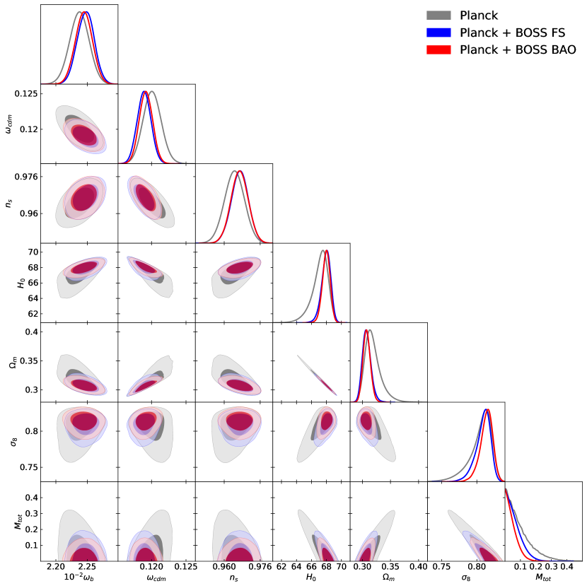
Figure 1: Marginalized one-dimensional posterior distribution and two-dimensional probability contours (at the 68% and 95% CL) for the parameters of the $\Lambda$CDM model with varied neutrino masses. $N_{\text{eff}}$ is fixed to the standard model value $3.046$. $H_{0}$ is quoted in km/s/Mpc, $M_{\text{tot}}$ is quoted in eV.

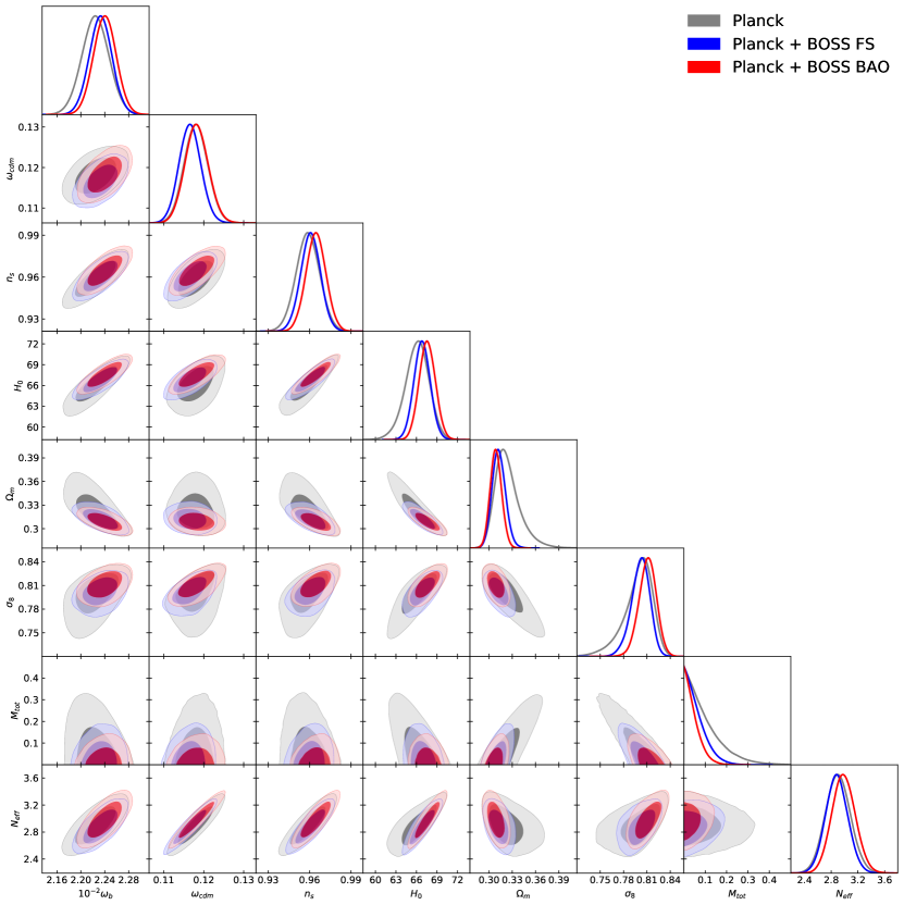
Figure 2: Marginalized one-dimensional posterior distribution and two-dimensional probability contours (at the 68% and 95% CL) for the parameters of the $\Lambda$CDM model with both varied neutrino masses and the effective number of relativistic degrees of freedom $N_{\text{eff}}$. $H_{0}$ is quoted in km/s/Mpc, $M_{\text{tot}}$ is quoted in eV.

3 Results

The triangle plots with posterior densities and marginalized distributions for cosmological parameters of the $\nu\Lambda$CDM model ($\omega_{b},\omega_{cdm},n_{s},H_{0},\Omega_{m},\sigma_{8},M_{\text{tot}}$) are shown in Fig. 1. A similar plot obtained for a model with free $N_{\text{eff}}$ (dubbed as $\nu\Lambda$CDM + $N_{\text{eff}}$) is displayed in Fig. 2. For comparison, we also show the contours obtained by analyzing the Planck data only. Results of this analysis are in good agreement with the ones reported by the Planck collaboration Aghanim et al. (2018). The marginalized limits are presented in Table 1.

The BOSS data notably improve the limits on the late-time parameters $H_{0}$, $\Omega_{m}$, $\sigma_{8}$, and the neutrino mass $M_{\text{tot}}$. This happens mainly due to the breaking of degeneracies between $H_{0}$ and other cosmological parameters in the CMB likelihood. This is not surprising, as the precision of $H_{0}$ measurement from the BOSS FS data alone rivals that of the CMB. The main improvement on the sum of neutrino masses brought by the BOSS data also comes from a better $H_{0}$ determination (this result was foreseen long ago in Ref. Hamann et al. (2010)). $H_{0}$ and $M_{\text{tot}}$ are anticorrelated in the CMB data, and the BOSS likelihood pulls $H_{0}$ to slightly higher values Ivanov et al. (2019), which pushes the neutrino masses closer to the origin. However, the BOSS data at the same time prefer a somewhat low value of $\sigma_{8}$ Ivanov et al. (2019) which pulls the neutrino masses in the opposite direction. This is reflected in our $95\%$ CL limit $0.16$ eV, which is higher than the Planck + BAO measurement $0.12$ eV. We stress that this relaxation does not imply that the FS data has less statistical power than the BAO. On the contrary, it is a result of taking into account new information that the BOSS clustering amplitude is lower than the Plank + BAO prediction.

It is instructive to see how much the neutrino mass bounds depend on the priors. Following the Planck methodology, we have imposed an unphysical zero lower limit in our baseline analysis. However, the physical priors corresponding to the normal or inverted hierarchies (NH and IH in what follows, respectively) can notably change the result. To estimate this effect we have resampled our chains with the physical lower priors ($0.06$ eV for DH and $0.1$ eV for IH) and obtained the following bounds (at 95$\%$CL):

$$\begin{split}&M_{\text{tot}}<0.18\,\text{eV}\quad(\text{NH, Planck~{}+~{}FS})\,,\\ &M_{\text{tot}}<0.21\,\text{eV}\quad(\text{IH, Planck~{}+~{}FS})\,.\\ \end{split}$$ (2)

These values can be compared with the Planck + BAO results which were extracted from our chains by a similar resampling,

$$\begin{split}&M_{\text{tot}}<0.15\,\text{eV}\quad(\text{NH, Planck~{}+~{}BAO})\,,\\ &M_{\text{tot}}<0.18\,\text{eV}\quad(\text{IH, Planck~{}+~{}BAO})\,.\\ \end{split}$$ (3)

As far as the base cosmological parameters are concerned, the improvement from the FS data (which embody the unreconstructed BAO) for $\nu\Lambda$CDM is comparable to that from the reconstructed BAO measurements Aghanim et al. (2018). This reflects the fact that the shape of the matter power spectrum does not contribute significantly to the cosmological constraints on the physical densities of baryons and dark matter, which are dominated by Planck.

One may expect that the shape information can be more important is the model with additional relativistic degrees of freedom. However, in this model the CMB degeneracy direction in the plane $\omega_{cdm}-H_{0}$ changes its orientation compared to the base $\Lambda$CDM and accidentally becomes aligned with the degeneracy direction of the BOSS data. Due to this coincidence the parameter degeneracies from the two datasets do not get broken, and the improvement from their combination is quite modest. Importantly, the posterior contour in the $\omega_{cdm}-H_{0}$ plane is shifted down as a consequence of the preference of the BOSS data for low $\omega_{cdm}$ Ivanov et al. (2019). This also produces some $\sim 0.5\sigma$ shifts in cosmological parameters as compared to the Planck + BAO analysis. In particular, we find

$$\begin{aligned} N_{\text{eff}}&=2.88\pm 0.17\\ H_{0}&=66.8\pm 1.2\end{aligned}\Bigg{\}}\quad\begin{aligned} \text{(68 $\%$, Planck~{}+~{}FS),}\\ \end{aligned}$$ (4)

which can be contrasted with

$$\begin{aligned} N_{\text{eff}}&=2.99\pm 0.17\\ H_{0}&=67.6\pm 1.2\end{aligned}\Bigg{\}}\quad\begin{aligned} \text{(68 $\%$, Planck~{}+~{}BAO),}\\ \end{aligned}$$ (5)

where $H_{0}$ is quoted in km/s/Mpc. Note that the FS and the BAO data pull the mean of $N_{\text{eff}}$ in different directions. Moreover, unlike the FS data, the BAO notably shift the means of other parameters, e.g. $\omega_{cdm}$ and $H_{0}$. This shows that the full-shape and BAO data: (i) Contain different information, (ii) Have similar statistical powers in combination with Planck. The interpretation of these results is that most of the improvement in the joint constraint comes from breaking of geometric degeneracy between $H_{0}$ and other cosmological parameters. Both the BAO and FS have the same amount of geometric information that primarily constrains $H_{0}$ for the models that we considered Ivanov et al. (2019), and hence the errorbars are very similar. However, the additional shape and clustering amplitude information contained in the FS data are not negligible, and their addition leads to $\sim 0.5\sigma$ shifts of the Planck + FS posteriors compared to Planck + BAO.

Finally, let us remark that we varied $N_{\text{eff}}$ together with the neutrino mass, but this choice does not degrade our limits compared to a fit with fixed $M_{\text{tot}}$. The reason is that the Planck data itself clearly distinguish between the two effects because the errorbars from the joint $M_{\text{tot}}~{}+~{}N_{\text{eff}}$ fit are the same as in the individual $M_{\text{tot}}$ and $N_{\text{eff}}$ runs Aghanim et al. (2018). This is also true for the BOSS likelihood, as we have obtained identical constraints on $M_{\text{tot}}$ that are twice stronger than Planck both with fixed and varied $N_{\text{eff}}$. This suggests that the two effects are clearly discriminated by the BOSS data too.

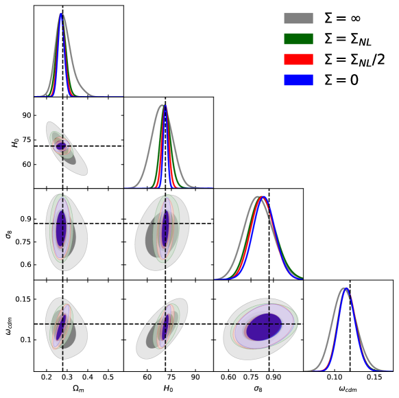
Figure 3: Marginalized one-dimensional posterior distribution and two-dimensional probability contours (at the 68% and 95% CL) for the parameters of simulated mock BOSS data. The shown are four cases corresponding to different amount of the BAO smoothing, see the main text for further details.

4 Wiggles vs. Broadband

In the previous Section we have presented results for the two different analyses, Planck + BAO and Planck + FS. As argued in Introduction, the information extracted form the galaxy clustering in these two methods is quite different, yet the error bars in the two analyses are identical. This is a very striking feature of our results and it requires an explanation. In this section we investigate the information content in the BAO and FS analyses in detail and show that the identical error bars are just a coincidence for the given volume of the BOSS survey and the given BAO reconstruction efficiency. We will argue that for larger future spectroscopic surveys the FS analysis will eventually be more powerful in constraining the cosmological parameters.

In order to compare the amount of information in the reconstructed BAO wiggles with the amount of information in the full shape power spectrum (which embeds the unreconstructed BAO), we analyzed several sets of the simulated mock data which mimic the actual BOSS sample, but have different amplitudes of the BAO wiggles. This exercise is analogous to that performed in Ref. Ivanov et al. (2019), where one can find further details of our mock dataset. We generated four sets of power spectra multipoles for the low-z ($z_{\text{eff}}=0.38$) DR12 North Galactic Cap (NGC) sample with a different amount of the BAO damping and analyzed them using the same pipeline appropriately modified in each case. The mock data were assigned the covariance of the real sample. For clarity, we analyze the mock BOSS data per se, i.e. without the Planck likelihood.

To understand our method, recall that the BAO damping at leading order can be described as

$$P_{\text{IR res, LO}}(k,\mu)=P_{\text{nw}}+{\rm e}^{-\Sigma^{2}k^{2}}P_{\text{w}}\,,$$ (6)

where $P_{\text{nw}}$ and $P_{\text{w}}$ are the de-wiggled broadband and wiggly parts of the linear power spectrum respectively. We also introduced $\mu\equiv\cos({\bf z},\bf k)$, where ${\bf z}$ is the line-of-sight vector. The theoretical prediction for the damping factor $\Sigma$ is given by Baldauf et al. (2015); Blas et al. (2016b); Ivanov and Sibiryakov (2018),

$$\begin{split}&\Sigma^{2}=\Sigma^{2}_{\text{NL}}\equiv(1+f\mu^{2}(2+f))\\ &\times\frac{4\pi}{3}\int_{0}^{k_{S}}dqP_{\text{nw}}(q)\left[1-j_{0}\left(qr_{d}\right)+2j_{2}\left(qr_{d}\right)\right]\,,\end{split}$$ (7)

where $f$ is the logarithmic growth factor, $j_{\ell}(x)$ are spherical Bessel functions, $k_{S}$ is an arbitrary scale separating the resummed soft modes and $r_{d}$ is the sound horizon at the drag epoch. We emphasize that the leading order expression (6) has a non-negligible dependence on $k_{S}$, which greatly reduces after computing the one-loop correction to Eq. (6) Blas et al. (2016b). Note that we use Eq. (6) only for illustration purposes. In the actual analysis we compute the full one-loop IR resummed expression with appropriately modified values of $\Sigma$.

The four mock samples are characterized by four different BAO damping factors $\Sigma=\infty,\Sigma_{\text{NL}},\Sigma_{\text{NL}}/2,0$, where $\Sigma_{\text{NL}}$ is the theoretically predicted amount of the BAO damping (7). The first case corresponds to the pure broadband information without any wiggles. The second case mimics the real physical situation and reproduces the actual constraints from the FS analysis of the BOSS low-z NGC data sample. The third situation corresponds to the combination of the broadband with the standard BAO reconstruction, which reduces the damping by a factor of two Beutler et al. (2017b). Finally, the fourth scenario features the full BAO wiggles, which are not affected by the non-linear smearing. This case corresponds to the joint analysis the broadband + optimally reconstructed BAO wiggles, which is the best case scenario for BAO reconstruction.

Param.	$\Sigma=\infty$	$\Sigma=\Sigma_{\text{NL}}$	$\Sigma=\Sigma_{\text{NL}}/2$	$\Sigma=0$
$\omega_{cdm}$	$0.112_{-0.015}^{+0.014}$	$0.116_{-0.011}^{+0.010}$	$0.116_{-0.011}^{+0.010}$	$0.116_{-0.011}^{+0.010}$
$H_{0}$	$69.3^{+6.3}_{-6.1}$	$71.4^{+2.9}_{-3.4}$	$71.3^{+1.9}_{-2.1}$	$71.3^{+1.2}_{-1.4}$
$\sigma_{8}$	$0.802_{-0.100}^{+0.091}$	$0.828_{-0.092}^{+0.082}$	$0.828_{-0.075}^{+0.076}$	$0.837_{-0.071}^{+0.072}$
$\Omega_{m}$	$0.284^{+0.031}_{-0.074}$	$0.271^{+0.021}_{-0.021}$	$0.271^{+0.017}_{-0.018}$	$0.271^{+0.015}_{-0.016}$

Table 2: Mean values and 68% CL minimum credible intervals for the parameters extracted from the simulated data mocking the BOSS DR12 low-z NGC sample. The values of $H_{0}$ are quoted in units of km/s/Mpc.

For the purposes of this Section, we focus on the following set of cosmological parameters ($H_{0},\omega_{cdm}$,$\sigma_{8}$) and use the Planck priors for $\omega_{b}$ and $n_{s}$. We fixed $M_{\text{tot}}=0$ in our simulated data. The chosen fitting parameters represent three different sources of information encoded in the power-spectrum multipoles: geometric distance ($H_{0}$), shape of the transfer functions ($\omega_{cdm}$), and redshift-space distortions ($\sigma_{8}$). The results of our analysis are displayed in Fig. 3 and Table 2. We also show the derived parameter $\Omega_{m}$, which comes from a combination of the shape and distance information.

The relative importance of the BAO wiggles compared to the broadband can be assessed comparing the results for the four different mock data sets. The first observation is that the BAO wiggles significantly affect only the $H_{0}$ measurement. There is no improvement in $\omega_{cdm}$ between the reconstructed and unreconstructed cases, and a very slight errorbar reduction for the clustering amplitude $\sigma_{8}$. The second observation is that the $H_{0}$ constraint improves by $\sim 40\%$ (i.e. the error reduces by $\sim\sqrt{2}$) in $\Sigma=\Sigma_{\text{NL}}/2$ compared to the $\Sigma=\Sigma_{\text{NL}}$ case. Thus, we can conclude that the reconstructed high-$k$ BAO wiggles measure $H_{0}$ with the similar precision as the FS data. This is precisely related to our result that the BAO and FS have a similar amount of geometric information. However, this is just a coincidence. Even small modifications in the setup can change the conclusions drastically. For example, in the case of the ideal BAO reconstruction the error on $H_{0}$ is smaller by more than a factor of $2$ compared to the standard FS analysis. This result suggests that $H_{0}$ errorbars are very sensitive to the efficiency of BAO reconstruction. While $\Sigma=0$ limit is probably impossible to get in practice, any improvement in the reconstruction algorithm can potentially be very important for the BOSS data analysis.

Another relevant parameter in this discussion is the volume of the survey. Smaller statistical errors can significantly improve the cosmological constraints thanks to the degeneracy breaking among many nuisance parameters needed to describe the broadband. Furthermore, larger surveys include higher redshifts, where the the BAO peak is much less damped. Thus, the expectation is that for large enough volumes, the FS should eventually win over the BAO-only analysis.

This is indeed the case. A similar mock analysis for a Euclid-like survey Chudaykin and Ivanov (2019) (whose volume is roughly 10 times larger than BOSS) has shown that even in the ideal case of the $100\%$-efficient BAO reconstruction the errorbar on $H_{0}$ improves only by $\lesssim 30\%$ compared to the FS constraints, which should be contrasted with the $\sim 100\%$ improvement for the BOSS volume. Repeating the analysis as Ref. Chudaykin and Ivanov (2019) for a more realistic case of $50\%$-efficient reconstruction we found the improvement for the Euclid data to be marginal ($\lesssim 10\%$), which can be contrasted with the $\sim 40\%$ gain for the BOSS volume. These results are not very surprising, and similar trends have been already seen in several other forecasts (see for instance BAO and broadband comparison in Aghamousa et al. (2016)).

In conclusion, comparing the amount of information in the BAO and FS analyses in detail, we find that the similarity between the two in combination with Planck is just a coincidence of the BOSS survey volume and efficiency of the current reconstruction algorithms. Our analysis suggests two main conclusions: (a) Better reconstruction algorithms or optimal combination of the FS and BAO analyses can lead to tighter constraints on cosmological parameters using the same BOSS data, (b) The full-shape power spectrum data will supersede the BAO measurements in the era of future galaxy surveys, even for in the case of ideal BAO reconstruction.

5 Conclusions

We have presented a joint analysis of the final Planck CMB and BOSS galaxy power spectrum data. Our main results include new limits on the parameters of the minimal $\Lambda$CDM, neutrino masses, and the number of effective relativistic degrees of freedom. The key new feature of our work is the use of a new BOSS full-shape power spectrum likelihood, which is based on an improved perturbation theory model. This model consistently accounts for nonlinearities of the underlying dark matter fluid, galaxy bias, redshift-space distortions, and nonlinear effects of large-scale bulk flows.

We showed that the addition of the BOSS FS data improves the Planck-only constraints. The results for the minimal $\Lambda$CDM with varied $M_{\text{tot}}$ are very similar to the standard Planck + BAO analysis. For the model with additional relativistic degrees of freedom the FS and BAO data yield comparable statistical improvement but shift the posterior in different directions. We argued that this is the effect of the additional full-shape information beyond the geometric location of the BAO.

When combined with Planck, the cosmological information in the shape of the BOSS galaxy power spectrum turned out to be comparable to the pure geometric information extracted form the reconstructed BAO peak for the cosmological models considered in this paper. However, the FS measurement will become more powerful than the BAO in the era of future galaxy surveys even for constraining vanilla cosmological scenarios. Importantly, the precision of the shape parameter measurements from these surveys will be comparable to that of Planck, and the combination of the two will reduce the errorbars by a factor of few due to degeneracy breaking Chudaykin and Ivanov (2019). This effect will be essential for the future neutrino mass measurements Audren et al. (2013a); Font-Ribera et al. (2014); Aghamousa et al. (2016); Archidiacono et al. (2017); Sprenger et al. (2019); Brinckmann et al. (2019); Chudaykin and Ivanov (2019). The presented constraints set a reference mark for future LSS and CMB observations that will surpass Planck and BOSS.

References

- Aghanim et al. (2018) N. Aghanim et al. (Planck), (2018), arXiv:1807.06209 [astro-ph.CO] .
- Alam et al. (2017) S. Alam et al. (BOSS), Mon. Not. Roy. Astron. Soc. 470, 2617 (2017), arXiv:1607.03155 [astro-ph.CO] .
- Eisenstein et al. (2007) D. J. Eisenstein, H.-j. Seo, E. Sirko, and D. Spergel, Astrophys. J. 664, 675 (2007), arXiv:astro-ph/0604362 [astro-ph] .
- Padmanabhan et al. (2009) N. Padmanabhan, M. White, and J. D. Cohn, Phys. Rev. D79, 063523 (2009), arXiv:0812.2905 [astro-ph] .
- Schmittfull et al. (2015) M. Schmittfull, Y. Feng, F. Beutler, B. Sherwin, and M. Y. Chu, Phys. Rev. D92, 123522 (2015), arXiv:1508.06972 [astro-ph.CO] .
- Schmittfull et al. (2017) M. Schmittfull, T. Baldauf, and M. Zaldarriaga, Phys. Rev. D96, 023505 (2017), arXiv:1704.06634 [astro-ph.CO] .
- Esteban et al. (2019) I. Esteban, M. C. Gonzalez-Garcia, A. Hernandez-Cabezudo, M. Maltoni, and T. Schwetz, JHEP 01, 106 (2019), arXiv:1811.05487 [hep-ph] .
- Palanque-Delabrouille et al. (2015) N. Palanque-Delabrouille et al., JCAP 1511, 011 (2015), arXiv:1506.05976 [astro-ph.CO] .
- Cuesta et al. (2016) A. J. Cuesta, V. Niro, and L. Verde, Phys. Dark Univ. 13, 77 (2016), arXiv:1511.05983 [astro-ph.CO] .
- Upadhye (2019) A. Upadhye, JCAP 1905, 041 (2019), arXiv:1707.09354 [astro-ph.CO] .
- Doux et al. (2018) C. Doux, M. Penna-Lima, S. D. P. Vitenti, J. Tréguer, E. Aubourg, and K. Ganga, Mon. Not. Roy. Astron. Soc. 480, 5386 (2018), arXiv:1706.04583 [astro-ph.CO] .
- Vagnozzi et al. (2017) S. Vagnozzi, E. Giusarma, O. Mena, K. Freese, M. Gerbino, S. Ho, and M. Lattanzi, Phys. Rev. D96, 123503 (2017), arXiv:1701.08172 [astro-ph.CO] .
- Palanque-Delabrouille et al. (2019) N. Palanque-Delabrouille, C. Yèche, N. Schöneberg, J. Lesgourgues, M. Walther, S. Chabanier, and E. Armengaud, (2019), arXiv:1911.09073 [astro-ph.CO] .
- Roy Choudhury and Hannestad (2019) S. Roy Choudhury and S. Hannestad, (2019), arXiv:1907.12598 [astro-ph.CO] .
- Aker et al. (2019) M. Aker et al. (KATRIN), (2019), arXiv:1909.06048 [hep-ex] .
- Ivanov et al. (2019) M. M. Ivanov, M. Simonovic, and M. Zaldarriaga, (2019), arXiv:1909.05277 [astro-ph.CO] .
- D’Amico et al. (2019) G. D’Amico, J. Gleyzes, N. Kokron, D. Markovic, L. Senatore, P. Zhang, F. Beutler, and H. Gil-Marín, (2019), arXiv:1909.05271 [astro-ph.CO] .
- Colas et al. (2019) T. Colas, G. D’amico, L. Senatore, P. Zhang, and F. Beutler, (2019), arXiv:1909.07951 [astro-ph.CO] .
- Tröster et al. (2019) T. Tröster et al., (2019), arXiv:1909.11006 [astro-ph.CO] .
- Beutler et al. (2017a) F. Beutler et al. (BOSS), Mon. Not. Roy. Astron. Soc. 466, 2242 (2017a), arXiv:1607.03150 [astro-ph.CO] .
- Abazajian et al. (2012) K. N. Abazajian et al., (2012), arXiv:1204.5379 [hep-ph] .
- Drewes et al. (2017) M. Drewes et al., JCAP 1701, 025 (2017), arXiv:1602.04816 [hep-ph] .
- Gil-Marín et al. (2015) H. Gil-Marín, L. Verde, J. Noreña, A. J. Cuesta, L. Samushia, W. J. Percival, C. Wagner, M. Manera, and D. P. Schneider, Mon. Not. Roy. Astron. Soc. 452, 1914 (2015), arXiv:1408.0027 [astro-ph.CO] .
- Beutler et al. (2014) F. Beutler et al. (BOSS), Mon. Not. Roy. Astron. Soc. 444, 3501 (2014), arXiv:1403.4599 [astro-ph.CO] .
- Grieb et al. (2017) J. N. Grieb et al. (BOSS), Mon. Not. Roy. Astron. Soc. 467, 2085 (2017), arXiv:1607.03143 [astro-ph.CO] .
- Sanchez et al. (2017) A. G. Sanchez et al. (BOSS), Mon. Not. Roy. Astron. Soc. 464, 1640 (2017), arXiv:1607.03147 [astro-ph.CO] .
- Amendola et al. (2018) L. Amendola et al., Living Rev. Rel. 21, 2 (2018), arXiv:1606.00180 [astro-ph.CO] .
- Aghamousa et al. (2016) A. Aghamousa et al. (DESI), (2016), arXiv:1611.00036 [astro-ph.IM] .
- Baumann et al. (2012) D. Baumann, A. Nicolis, L. Senatore, and M. Zaldarriaga, JCAP 1207, 051 (2012), arXiv:1004.2488 [astro-ph.CO] .
- Carrasco et al. (2012) J. J. M. Carrasco, M. P. Hertzberg, and L. Senatore, JHEP 09, 082 (2012), arXiv:1206.2926 [astro-ph.CO] .
- Senatore and Zaldarriaga (2014) L. Senatore and M. Zaldarriaga, (2014), arXiv:1409.1225 [astro-ph.CO] .
- Senatore (2015) L. Senatore, JCAP 1511, 007 (2015), arXiv:1406.7843 [astro-ph.CO] .
- Perko et al. (2016) A. Perko, L. Senatore, E. Jennings, and R. H. Wechsler, (2016), arXiv:1610.09321 [astro-ph.CO] .
- Chudaykin and Ivanov (2019) A. Chudaykin and M. M. Ivanov, (2019), arXiv:1907.06666 [astro-ph.CO] .
- Senatore and Zaldarriaga (2015) L. Senatore and M. Zaldarriaga, JCAP 1502, 013 (2015), arXiv:1404.5954 [astro-ph.CO] .
- Vlah et al. (2015) Z. Vlah, M. White, and A. Aviles, JCAP 1509, 014 (2015), arXiv:1506.05264 [astro-ph.CO] .
- Vlah et al. (2016) Z. Vlah, U. Seljak, M. Y. Chu, and Y. Feng, JCAP 1603, 057 (2016), arXiv:1509.02120 [astro-ph.CO] .
- Baldauf et al. (2015) T. Baldauf, M. Mirbabayi, M. Simonović, and M. Zaldarriaga, Phys. Rev. D92, 043514 (2015), arXiv:1504.04366 [astro-ph.CO] .
- Blas et al. (2016a) D. Blas, M. Garny, M. M. Ivanov, and S. Sibiryakov, JCAP 1607, 052 (2016a), arXiv:1512.05807 [astro-ph.CO] .
- Blas et al. (2016b) D. Blas, M. Garny, M. M. Ivanov, and S. Sibiryakov, JCAP 1607, 028 (2016b), arXiv:1605.02149 [astro-ph.CO] .
- Ivanov and Sibiryakov (2018) M. M. Ivanov and S. Sibiryakov, JCAP 1807, 053 (2018), arXiv:1804.05080 [astro-ph.CO] .
- Pueblas and Scoccimarro (2009) S. Pueblas and R. Scoccimarro, Phys. Rev. D80, 043504 (2009), arXiv:0809.4606 [astro-ph] .
- Lewandowski et al. (2015) M. Lewandowski, A. Perko, and L. Senatore, JCAP 1505, 019 (2015), arXiv:1412.5049 [astro-ph.CO] .
- Desjacques et al. (2018) V. Desjacques, D. Jeong, and F. Schmidt, Phys. Rept. 733, 1 (2018), arXiv:1611.09787 [astro-ph.CO] .
- Jackson (1972) J. C. Jackson, Mon. Not. Roy. Astron. Soc. 156, 1P (1972), arXiv:0810.3908 [astro-ph] .
- Lesgourgues and Pastor (2006) J. Lesgourgues and S. Pastor, Phys. Rept. 429, 307 (2006), arXiv:astro-ph/0603494 [astro-ph] .
- Di Valentino et al. (2018) E. Di Valentino et al. (CORE), JCAP 1804, 017 (2018), arXiv:1612.00021 [astro-ph.CO] .
- Brinckmann and Lesgourgues (2018) T. Brinckmann and J. Lesgourgues, (2018), arXiv:1804.07261 [astro-ph.CO] .
- Aghanim et al. (2019) N. Aghanim et al. (Planck), (2019), arXiv:1907.12875 [astro-ph.CO] .
- du Mas des Bourboux et al. (2017) H. du Mas des Bourboux et al., Astron. Astrophys. 608, A130 (2017), arXiv:1708.02225 [astro-ph.CO] .
- Ata et al. (2018) M. Ata et al., Mon. Not. Roy. Astron. Soc. 473, 4773 (2018), arXiv:1705.06373 [astro-ph.CO] .
- Feng et al. (2018) Y. Feng, U. Seljak, and M. Zaldarriaga, JCAP 1807, 043 (2018), arXiv:1804.09687 [astro-ph.CO] .
- Modi et al. (2018) C. Modi, Y. Feng, and U. Seljak, JCAP 1810, 028 (2018), arXiv:1805.02247 [astro-ph.CO] .
- Schmittfull et al. (2019) M. Schmittfull, M. Simonović, V. Assassi, and M. Zaldarriaga, Phys. Rev. D100, 043514 (2019), arXiv:1811.10640 [astro-ph.CO] .
- Schmidt et al. (2019) F. Schmidt, F. Elsner, J. Jasche, N. M. Nguyen, and G. Lavaux, JCAP 1901, 042 (2019), arXiv:1808.02002 [astro-ph.CO] .
- Elsner et al. (2019) F. Elsner, F. Schmidt, J. Jasche, G. Lavaux, and N.-M. Nguyen, (2019), arXiv:1906.07143 [astro-ph.CO] .
- Hahn et al. (2017) C. Hahn, R. Scoccimarro, M. R. Blanton, J. L. Tinker, and S. A. Rodríguez-Torres, Mon. Not. Roy. Astron. Soc. 467, 1940 (2017), arXiv:1609.01714 [astro-ph.CO] .
- Nicola et al. (2016) A. Nicola, A. Refregier, and A. Amara, Phys. Rev. D94, 083517 (2016), arXiv:1607.01014 [astro-ph.CO] .
- Blas et al. (2014) D. Blas, M. Garny, T. Konstandin, and J. Lesgourgues, JCAP 1411, 039 (2014), arXiv:1408.2995 [astro-ph.CO] .
- Senatore and Zaldarriaga (2017) L. Senatore and M. Zaldarriaga, (2017), arXiv:1707.04698 [astro-ph.CO] .
- Takada et al. (2006) M. Takada, E. Komatsu, and T. Futamase, Phys. Rev. D73, 083520 (2006), arXiv:astro-ph/0512374 [astro-ph] .
- Villaescusa-Navarro et al. (2014) F. Villaescusa-Navarro, F. Marulli, M. Viel, E. Branchini, E. Castorina, E. Sefusatti, and S. Saito, JCAP 1403, 011 (2014), arXiv:1311.0866 [astro-ph.CO] .
- Castorina et al. (2014) E. Castorina, E. Sefusatti, R. K. Sheth, F. Villaescusa-Navarro, and M. Viel, JCAP 1402, 049 (2014), arXiv:1311.1212 [astro-ph.CO] .
- Costanzi et al. (2013) M. Costanzi, F. Villaescusa-Navarro, M. Viel, J.-Q. Xia, S. Borgani, E. Castorina, and E. Sefusatti, JCAP 1312, 012 (2013), arXiv:1311.1514 [astro-ph.CO] .
- Castorina et al. (2015) E. Castorina, C. Carbone, J. Bel, E. Sefusatti, and K. Dolag, JCAP 1507, 043 (2015), arXiv:1505.07148 [astro-ph.CO] .
- Villaescusa-Navarro et al. (2018) F. Villaescusa-Navarro, A. Banerjee, N. Dalal, E. Castorina, R. Scoccimarro, R. Angulo, and D. N. Spergel, Astrophys. J. 861, 53 (2018), arXiv:1708.01154 [astro-ph.CO] .
- Raccanelli et al. (2019) A. Raccanelli, L. Verde, and F. Villaescusa-Navarro, Mon. Not. Roy. Astron. Soc. 483, 734 (2019), arXiv:1704.07837 [astro-ph.CO] .
- Vagnozzi et al. (2018) S. Vagnozzi, T. Brinckmann, M. Archidiacono, K. Freese, M. Gerbino, J. Lesgourgues, and T. Sprenger, JCAP 1809, 001 (2018), arXiv:1807.04672 [astro-ph.CO] .
- Kaiser (1987) N. Kaiser, Mon. Not. Roy. Astron. Soc. 227, 1 (1987).
- Chiang et al. (2018) C.-T. Chiang, W. Hu, Y. Li, and M. Loverde, Phys. Rev. D97, 123526 (2018), arXiv:1710.01310 [astro-ph.CO] .
- Chiang et al. (2019) C.-T. Chiang, M. LoVerde, and F. Villaescusa-Navarro, Phys. Rev. Lett. 122, 041302 (2019), arXiv:1811.12412 [astro-ph.CO] .
- Hamann et al. (2010) J. Hamann, S. Hannestad, J. Lesgourgues, C. Rampf, and Y. Y. Y. Wong, JCAP 1007, 022 (2010), arXiv:1003.3999 [astro-ph.CO] .
- Beutler et al. (2017b) F. Beutler et al. (BOSS), Mon. Not. Roy. Astron. Soc. 464, 3409 (2017b), arXiv:1607.03149 [astro-ph.CO] .
- Yankelevich and Porciani (2019) V. Yankelevich and C. Porciani, Mon. Not. Roy. Astron. Soc. 483, 2078 (2019), arXiv:1807.07076 [astro-ph.CO] .
- Audren et al. (2013a) B. Audren, J. Lesgourgues, S. Bird, M. G. Haehnelt, and M. Viel, JCAP 1301, 026 (2013a), arXiv:1210.2194 [astro-ph.CO] .
- Font-Ribera et al. (2014) A. Font-Ribera, P. McDonald, N. Mostek, B. A. Reid, H.-J. Seo, and A. Slosar, JCAP 1405, 023 (2014), arXiv:1308.4164 [astro-ph.CO] .
- Archidiacono et al. (2017) M. Archidiacono, T. Brinckmann, J. Lesgourgues, and V. Poulin, JCAP 1702, 052 (2017), arXiv:1610.09852 [astro-ph.CO] .
- Sprenger et al. (2019) T. Sprenger, M. Archidiacono, T. Brinckmann, S. Clesse, and J. Lesgourgues, JCAP 1902, 047 (2019), arXiv:1801.08331 [astro-ph.CO] .
- Brinckmann et al. (2019) T. Brinckmann, D. C. Hooper, M. Archidiacono, J. Lesgourgues, and T. Sprenger, JCAP 1901, 059 (2019), arXiv:1808.05955 [astro-ph.CO] .
- Blas et al. (2011) D. Blas, J. Lesgourgues, and T. Tram, JCAP 1107, 034 (2011), arXiv:1104.2933 [astro-ph.CO] .
- Audren et al. (2013b) B. Audren, J. Lesgourgues, K. Benabed, and S. Prunet, JCAP 1302, 001 (2013b), arXiv:1210.7183 [astro-ph.CO] .
- Simonovic et al. (2018) M. Simonovic, T. Baldauf, M. Zaldarriaga, J. J. Carrasco, and J. A. Kollmeier, JCAP 1804, 030 (2018), arXiv:1708.08130 [astro-ph.CO] .
- Lewis and Bridle (2002) A. Lewis and S. Bridle, Phys. Rev. D66, 103511 (2002), arXiv:astro-ph/0205436 [astro-ph] .
- Lewis (2013) A. Lewis, Phys. Rev. D87, 103529 (2013), arXiv:1304.4473 [astro-ph.CO] .