NLO Massive Event-Shape Differential and Cumulative Distributions

Abstract

We provide a general method to effectively compute differential and cumulative event-shape distributions to $\mathcal{O}(\alpha_{s})$ precision for massive quarks produced primarily at an $e^{+}e^{-}$ collider. In particular, we show that at this order, due to the screening of collinear singularities by the quark mass, for all event shapes linearly sensitive to soft dynamics, there appear only two distributions at threshold: a Dirac delta function and a plus distribution. Furthermore, we show that the coefficient of the latter is universal for any infra-red and collinear safe event shape, and provide an analytic expression for it. Likewise, we compute a general formula for the coefficient of the Dirac delta function, which depends only on the event-shape measurement function in the soft limit. Finally, we present an efficient algorithm to compute the differential and cumulative distributions, which does not rely on Monte Carlo methods, therefore achieving a priory arbitrary precision even in the extreme dijet region. We implement this algorithm in a numeric code and show that it agrees with analytic results on the distribution for 2-jettiness, heavy jet mass and a massive generalization of C-parameter.

1 Introduction

Recent years have seen tremendous progress in the understanding and computation of event-shape cross sections for $e^{+}e^{-}$ machines such as LEP or the future linear and circular colliders. This is mainly achieved with the use of factorized expressions (see e.g. Refs. Schwartz:2007ib ; Bauer:2008dt ) derived in the frame of the effective field theory (EFT) known as Soft-Collinear Effective Theory (SCET) Bauer:2000ew ; Bauer:2000yr ; Bauer:2001ct ; Bauer:2001yt ; Bauer:2002nz . The state of the art for massless event shapes is next-to-next-to-leading-log (N²LL) Hornig:2009vb ; Becher:2012qc ; Bell:2018gce and next-to-next-to-next-to-leading-log (N³LL) Becher:2008cf ; Chien:2010kc ; Hoang:2014wka ; Moult:2018jzp ; HJM-theo . The computation of the soft function has been fully automatized analytically at ${\cal O}(\alpha_{s})$ in Ref. Hoang:2014wka and numerically at ${\cal O}(\alpha_{s}^{2})$ in Refs. Bell:2018vaa ; Bell:2018oqa (in those articles one can also find analytic results for some event shapes such as C-parameter). Analytic fixed-order perturbative predictions exist at ${\cal O}(\alpha_{s})$ for thrust, heavy jet mass (HJM) and C-parameter, while for other event shapes such as angularities or jet broadening, the cross sections can be expressed as a 1D numerical integral. Numerical results exist at ${\cal O}(\alpha_{s}^{2})$ Catani:1996vz ; Dixon:2018qgp and ${\cal O}(\alpha_{s}^{3})$ GehrmannDeRidder:2007bj ; GehrmannDeRidder:2007hr ; Weinzierl:2008iv ; Ridder:2014wza ; Weinzierl:2009ms ; DelDuca:2016ily . In Ref. Mateu:2013gya the fixed-order cross sections for oriented event shapes have been computed up to ${\cal O}(\alpha_{s}^{2})$. These results have been used, in particular, to determine the strong coupling constant with very high precision Becher:2012qc ; Chien:2010kc ; Abbate:2010xh ; Abbate:2012jh ; Gehrmann:2012sc ; Hoang:2015hka ; HJM-fit .

The theoretical knowledge for event shapes involving massive quarks is comparatively much poorer. Fixed-order predictions have been obtained numerically at ${\cal O}(\alpha_{s})$ (analytic results at this order exist but are scarce) and ${\cal O}(\alpha_{s}^{2})$ Nason:1997nw ; Bernreuther:1997jn ; Rodrigo:1999qg . Factorization and resummation for 2-jettiness with massive quarks Fleming:2007xt ; Fleming:2007qr has recently achieved N³LL precision through the computation of matrix elements at two loops Jain:2008gb ; Gritschacher:2013pha ; Pietrulewicz:2014qza ; Hoang:2015vua ; Hoang:2019fze . These results have been used in Ref. Butenschoen:2016lpz to calibrate the Pythia 8.205 Sjostrand:2007gs top quark mass parameter in terms of the short-distance MSR scheme Hoang:2008yj ; Hoang:2017suc . In this direction, further theoretical progress has been made, and a $p_{T}$ cutoff as implemented in angular ordered parton showers has been included in Ref. Hoang:2018zrp . Event-shapes for massive particles shall play an important role at the future linear collider, where they will presumably be used to determine the top quark mass from boosted events in a well defined scheme within quantum field theory. This measurement is complementary to threshold scans with partially orthogonal experimental uncertainties. Furthermore, from the conclusions that can be drawn from this article, they might also be a useful tool to determine the strong coupling $\alpha_{s}$.

For a complete description of massive event shapes with N²LL accuracy in the peak region where the SCET and bHQET effective theories can be applied, but also valid in the tail and far-tail of the distribution, the resummed cross section has to be matched to the fixed-order prediction at $\mathcal{O}(\alpha_{s})$. In full generality, the differential cross section for massive particles up to this order can be written as

$$\frac{1}{\sigma^{C}_{0}}\frac{\mathrm{d}\sigma_{C}}{\mathrm{d}e}={} R^{0}_{C}(\hat{m})\,\delta(e-e_{\rm min})+C_{F}\frac{\alpha_{s}}{\pi}A^{C}_{e}({\hat{m}})\delta(e-e_{\rm min})$$ (1)

$$+C_{F}\frac{\alpha_{s}}{\pi}B^{C}_{\rm plus}({\hat{m}})\biggl{[}\frac{1}{e-e_{\rm min}}\biggr{]}_{+}+C_{F}\frac{\alpha_{s}}{\pi}F^{\rm NS}_{e}(e,\hat{m})+\mathcal{O}(\alpha_{s}^{2})\,,$$

with $F^{\rm NS}_{e}$ a function regular at $e_{\rm min}$, the lower endpoint of the distribution, $\sigma^{C}_{0}$ the massless Born-cross section and $R^{0}_{C}$ the tree level R-ratio. The sub- and super-scripts $C$ denote the type of current considered (vector or axial-vector), omitted for $F_{e}^{\mathrm{NS}}$ to keep the notation simple. In this paper we compute the differential and cumulative cross sections for all event shapes, for both vector and axial-vector currents, reaching the same standard as for massless quarks at this order (where essentially all results are known analytically in terms of relatively simple expressions), by obtaining analytical results for $A_{e}$ and $B_{\rm plus}$, and computing $F^{\rm NS}_{e}$ through 1-dimensional numerical integrals in a way which is almost as precise and stable as for a full analytic result. Our calculation shows that $A_{e}$ and $F^{\rm NS}_{e}$ depend on the specific event-shape variable, and $B_{\rm plus}$ is a universal function of the reduced mass $\hat{m}\equiv m/Q$. This matching program has already been carried out in previous work Butenschoen:2016lpz in a less efficient way. While at the time of the “NLO revolution” the $\mathcal{O}(\alpha_{s})$ results seem completely standard, having a dedicated article on those is still useful because: a) known results are mainly numeric and provided as binned distributions, which makes the matching to resummed results unpractical, b) analytic results are faster and easier to implement; c) non-zero quark masses entail that different event-shape schemes can be used, allowing to control the sensitivity to the mass, to the best of our knowledge a possibility never discussed so far; d) new strategies to efficiently compute the cross section are presented, which we believe will be useful for future work; e) our results are an important input for further studies of massive event shapes, which aim to improve our understanding of heavy quark mass determinations in general. This article provides all ingredients that are needed for a full N²LL computation in a way which is useful and easy to implement, and in that sense it will be a reference for many future analysis in this field. In particular our results will help to clarify the top quark Monte Carlo (MC) mass interpretation problem.

This article is organized as follows: in Sec. 2 we introduce massive schemes, and show how to implement them into massive event shapes. In Sec. 3 we provide a direct computation of our main analytic result, $A_{e}$, the coefficient of the delta function, computing the real and virtual contributions directly, canceling the infrared singularities explicitly. Sec. 4 deals with $F_{e}^{\rm NS}$, describing our numerical algorithm, which is applied to differential and cumulative cross sections as well as moments. Analytic results for cross sections of a few event shapes are shown in Sec. 5. Our conclusions are summarized in Sec. 7. We provide a second analytic computation of the delta-function coefficient in Appendix A, requiring that the integration of the differential cross section over its entire physical range reproduces the total hadronic cross section. Applications of our master formula for a selection of event shapes, analytic formulae for the massive total hadronic cross section and some master integrals are provided in the remaining appendices.

2 Event Shapes for Massive Particles

In this section we introduce generalizations of classic event shapes for massive heavy quarks, for which we present analytic results of the delta-function coefficient in Appendix D. These generalizations go under the name of  “mass schemes”, and have no effect on the partonic cross section for massless particles, but for massive quarks dramatically modify the sensitivity to their mass already at parton level even at the lowest order. This control on the sensitivity to the mass is of high interest, and in particular sets the effective renormalization scale of the heavy quark mass. No systematic study of these schemes exists yet for massive quarks, and here we intend to fill this gap.

Mass schemes for event shapes were originally introduced to study non-perturbative power corrections in the context of non-zero hadron masses Salam:2001bd ; Mateu:2012nk . In the case of massless quarks, partonic cross sections are unaffected by scheme changes, but power corrections substantially depend on the scheme choice. In particular it has been shown that the leading non-perturbative power correction is universal for the so-called E-scheme. They have been also used to study power corrections in the dressed-gluon approximation Gardi:2003iv and to determine the mass of heavy quarks in boosted events Fleming:2007qr . Due to increasing theoretical and experimental precision, it is necessary to include the finite bottom quark mass in high-precision calculations, e.g. for extracting the strong coupling constant Abbate:2010xh . On the other hand, mass effects are dominant and have to be included when extracting the quark mass itself or when carrying out mass-related studies such as analyzing the properties of the top quark Monte Carlo mass parameter.

When using classical event shapes like thrust, C-parameter, jet broadening etc. in presence of massive quarks, the way how one treats energies and three-momenta magnitudes is important, since (unlike for massless particles) $E_{p}\neq|\vec{p}\,|$. To categorize different ways of how to treat energies and three-momenta, several “schemes” can be defined for massive event shapes, which are distinguished exactly by the way how $E_{p}$ and $|\vec{p}\,|$ are interpreted. Obviously, all these schemes reduce to the original definition in the massless case.

Starting from the original definition of event shapes, the “E-scheme” is defined by the replacement $\vec{p}\to(E_{p}/|\vec{p}\,|)\,\vec{p}$, while the “P-scheme” is defined by the substitution $E_{p}\to|\vec{p}\,|$. Some event shapes originally defined in P-scheme are thrust Farhi:1977sg ,

$$\tau\equiv\tau^{P}=\frac{1}{Q_{P}}\sum_{i}p_{i,\bot}\mathrm{e}^{-|\eta_{i}|}=\frac{1}{Q_{P}}\min_{\hat{t}}\sum_{i}(|\vec{p}_{i}|-|\hat{t}\cdot\vec{p}_{i}|)\,,$$ (2)

C-parameter Parisi:1978eg ; Donoghue:1979vi (it is often useful to define the reduced C-parameter as $\widetilde{C}=C/6$)

$$C\equiv C^{P}=\frac{3}{2Q_{P}^{2}}\sum_{i,j}|\vec{p}_{i}||\vec{p}_{j}|\sin^{2}\theta_{ij}=\frac{3}{2}\biggl{[}1-\frac{1}{Q_{P}^{2}}\sum_{i,j}\frac{(\vec{p}_{i}\cdot\vec{p}_{j})^{2}}{|\vec{p}_{i}||\vec{p}_{j}|}\biggr{]}\,,$$ (3)

and broadening Rakow:1981qn

$$B_{T}\equiv B_{T}^{P}=\frac{1}{2Q_{P}}\sum_{i}p_{i,\bot}=\frac{1}{2Q_{P}}\sum_{i}(|\vec{p}_{i}|-|\hat{t}\cdot\vec{p}_{i}|)^{1/2}(|\vec{p}_{i}|+|\hat{t}\cdot\vec{p}_{i}|)^{1/2}\,,$$ (4)

while angularities Berger:2003pk were originally defined in the E-scheme:

$$\tau_{a}\equiv\tau_{a}^{E}=\frac{1}{Q}\sum_{i}\frac{E_{i}}{|\vec{p}_{i}|}p_{i,\bot}\mathrm{e}^{-|\eta_{i}|(1-a)}=\frac{1}{2Q}\sum_{i}\frac{E_{i}}{|\vec{p}_{i}|}(|\vec{p}_{i}|-|\hat{t}\cdot\vec{p}_{i}|)^{1-\frac{a}{2}}(|\vec{p}_{i}|+|\hat{t}\cdot\vec{p}_{i}|)^{\frac{a}{2}}\,,$$ (5)

where $\eta$ denotes the pseudo-rapidity, $p_{\bot}\equiv|\vec{p}_{\bot}|$ the transverse momentum measured with respect to the thrust axis, and $m_{\bot}\equiv\sqrt{p_{\bot}^{2}+m^{2}}$ is the transverse mass.

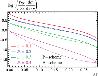
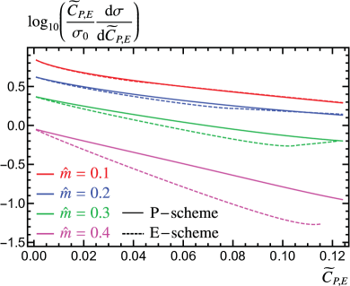
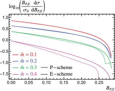
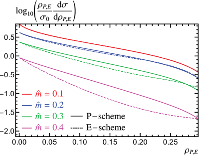
Figure 1: Event-shape differential distributions for the vector current in the P (solid lines) and E schemes (dashed lines). Panels (a), (b), (c), and (d) show the cross section for thrust, C-parameter, jet broadening, and heavy jet mass, respectively. All curves are multiplied by $e-e_{\rm min}$, with $e$ the event-shape value and $e_{\rm min}$ its minimal value, such that the cross section is finite for $e=e_{\rm min}$. Red, blue, green and magenta show the results for $\hat{m}=0.1,\,0.2,\,0.3$ and $0.4$, respectively.

The P-scheme version of angularities and E-scheme versions of the other event shapes listed here can be found in Appendix D. Note that the substitutions have to be done for the event-shape normalization as well, such that E-scheme event shapes are usually normalized using $Q=\sum_{i}E_{p,i}$, while P-scheme event shapes are normalized by $Q_{P}=\sum_{i}|\vec{p}_{i}|$. The definition of the thrust axis itself does not change with the scheme, i.e. it is always defined with respect to the original P-scheme thrust definition. The minimal value for these event shapes remains $e_{\rm min}=0$, meaning that these observables are insensitive to parton masses at leading order, which can be useful in cases where mass effects are preferred to be small.

Some event shapes are, in their original definitions, neither P- nor E-scheme, sometimes referred to as “massive scheme” or “M-scheme”, usually containing full momentum information . One of these is heavy jet mass Clavelli:1979md ; Chandramohan:1980ry ; Clavelli:1981yh , defined as the heavier of the two hemisphere invariant masses, normalized by $Q^{2}$

$$\rho=\frac{1}{Q^{2}}\Biggl{(}\,\sum_{i\in\text{heavy}}\!\!p_{i}\!\Biggr{)}^{\!\!2}\,,$$ (6)

where the hemispheres are defined to be separated by the plane orthogonal to the thrust axis. It can be useful to define massive scheme versions of other event shapes as well. Examples include the massive version of thrust (2-jettiness) Stewart:2009yx and C-parameter (C-jettiness) Gardi:2003iv . 2-jettiness is defined by generalizing the original definition to

$$\tau_{J}=\frac{1}{Q}\sum_{i}(|E_{i}|-|\hat{t}\cdot\vec{p}_{i}|)\,,$$ (7)

while C-jettiness is based on the Lorentz-invariant form

$$C_{J}=\frac{3}{2}\biggl{[}2-\sum_{i\neq j}\frac{(p_{i}\cdot p_{j})^{2}}{(p_{i}\cdot q)(p_{j}\cdot q)}\biggr{]},$$ (8)

introduced in Ref. Ellis:1980nc , with $q=\sum_{i}p_{i}$. These event shapes usually have a non-zero minimal value $e_{\rm min}\neq 0$ and are therefore mass sensitive already at leading order. The increased mass sensitivity can be useful when studying mass related issues, e.g. 2-jettiness was used to calibrate the Pythia 8.205 MC top quark mass Butenschoen:2016lpz and has been proposed to measure the top quark mass at a future linear collider Fleming:2007qr .

In Appendix D we present some analytic results for the delta-function coefficients of differential cross sections for the event shapes listed above in various schemes, together with respective characteristic information on the event shapes.

Differential cross sections in the E- and P-schemes for a selection of event shapes can be seen in Fig. 1. The plots have been generated using the algorithm described in Sec. 4.3. We do not show massive-scheme cross sections in this plot since their lower endpoint is different from zero. We have chosen the plot-range of the P-scheme allowed values, since they are mass-independent, and our $y$ axis is in a logarithmic scale to make the curves with small values of $\hat{m}$ visible. In general E-scheme maximal values do depend on the reduced mass (see Appendix D for some examples). Since the scheme dependence vanishes for $m=0$, curves are very similar for small values of the reduced mass, resulting in nearly identical red lines in all four panels of the figure. As the mass increases, the differences grow, and for $\hat{m}=0.4$ the curves in both schemes are clearly different. We observe that the cross section is smaller in the E-scheme for most of the spectrum.

3 Analytic Results for the Distributions at Threshold

Figure 2: Diagrammatic contribution to the $\mathcal{O}(\alpha_{s}^{0})$ differential event shape distribution. The diagram has to be squared and contributes only as a Dirac delta function.

In this section we provide the computation of one of our main results, an integral expression for the delta-function coefficient of event-shape differential cross sections in full QCD. Obviously, the results are different for vector and axial-vector currents, but the computation is analogous to both processes. Along the computation we show that the coefficient of the plus distribution is the same for any observable linearly sensitive to soft momentum. The delta-function coefficient receives contributions from the virtual- and real-radiation diagrams, which are separately IR divergent, although the sum is finite. The Feynman diagrams at LO and NLO are shown in Figs. 2 and 3, respectively. In the virtual term, the divergence originates from a loop integration, while in the real-radiation it is a consequence of the phase-space integration. The cancellation can be achieved by computing the two terms explicitly, as in the approach followed in Sec. 3.3 for the differential cross section, or, in the case of inclusive quantities such as the total hadronic cross section, by taking the imaginary part of the forward scattering amplitude. In this approach, IR divergences that might appear in individual Feynman diagrams are always a consequence of loop integrals. Furthermore, one never has to deal with squaring matrix elements. We exploit this fact in Appendix A, and analytically compute the delta-function coefficient by simply imposing that the differential cross section integrated across the whole spectrum reproduces the total hadronic cross section.

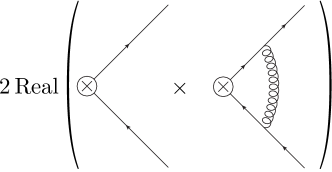
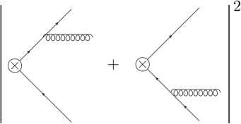
Figure 3: Contributions to the $\mathcal{O}(\alpha_{s})$ differential cross section for event shapes. Panel (a) shows the virtual contribution as twice the interference of the three-level and one one-loop diagrams, while in panel (b) the two real-radiation diagrams that have to be added and squared are drawn.

3.1 Born Cross Section and $\mathcal{O}(\alpha_{s}^{0})$ Distribution

It is customary to present event-shape distributions normalized to the Born cross section, which is defined as the cross section for massless quarks at tree-level in four dimensions. The Born cross section is different for vector and and axial-vector currents: the former gets contributions from both photon and Z-boson exchange, while the letter is mediated by the Z boson only. Taking into account the finite width $\Gamma_{Z}$ of the Z boson, one obtains

$$\sigma^{V}_{0} =\frac{N_{c}}{3}\frac{4\pi\alpha_{\rm em}^{2}}{Q^{2}}\Biggl{[}Q^{2}_{q}+\frac{v^{2}_{f}(v_{e}^{2}+a_{e}^{2})}{(1-\hat{m}_{Z}^{2})^{2}+\bigl{(}\frac{\Gamma_{Z}}{m_{Z}}\bigr{)}^{2}}+\frac{2\,Q_{q}v_{e}v_{q}(1-\hat{m}_{Z}^{2})}{(1-\hat{m}^{2}_{Z})^{2}+\bigl{(}\frac{\Gamma_{Z}}{m_{Z}}\bigr{)}^{2}}\Biggr{]},$$ (9)

$$\sigma^{A}_{0} =\frac{N_{c}}{3}\frac{4\pi\alpha_{\rm em}^{2}}{Q^{2}}\Biggl{[}\frac{a_{q}^{2}(v_{e}^{2}+a_{e}^{2})}{(1-\hat{m}_{Z}^{2})^{2}+\bigl{(}\frac{\Gamma_{Z}}{m_{Z}}\bigr{)}^{2}}\Biggr{]},$$

with $\alpha_{\rm em}$ the electromagnetic coupling, $\hat{m}_{Z}=m_{Z}/Q$ the reduced Z-boson mass, $Q_{q}$ the quark electric charge, $N_{c}$ the number of colors, and $v_{e}$ and $a_{e}$ ($v_{q}$ and $a_{q}$) the electron (quark) vector and axial-vector couplings to the Z boson. Here and in what follows, the leptonic trace is always computed in four dimensions. This poses no problem since we are taking the electroweak interactions at leading order only. For non-zero quark masses, the normalized tree-level cross section is different for vector and axial-vector currents:

$$\frac{\sigma^{V}_{0,m}}{\sigma^{V}_{0}}\equiv R_{0}^{V}(\hat{m})=\frac{(3-v^{2})\,v}{2}\,,\qquad\frac{\sigma^{A}_{0,m}}{\sigma^{A}_{0}}\equiv R_{0}^{A}(\hat{m})=v^{3}\,,$$ (10)

with $v=\sqrt{1-4\hat{m}^{2}}$ the velocity of the on-shell massive quarks in the center of mass frame. The functions $R_{0}^{V}$ and $R_{0}^{A}$ are shown graphically as a function of $\hat{m}$ in Fig. 4. In the massless limit $R_{0}^{C}(v=1)=1$, while both vanish at threshold ($v\to 0$). At $\mathcal{O}(\alpha_{s}^{0})$ the differential cross section is obviously

$$\frac{1}{\sigma^{C}_{0}}\frac{\mathrm{d}\sigma_{0}}{\mathrm{d}e}=R_{0}^{C}(\hat{m})\,\delta(e-e_{\rm min})\,,$$ (11)

with $C=V,A$ for vector and axial-vector currents, respectively, and $e_{\rm min}$ the minimal value the event shape can take.

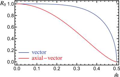
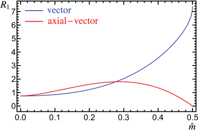
Figure 4: Massive total hadronic cross section for vector (blue) and axial-vector (red) currents, at tree-level in panel (a) and one loop in panel (b).

3.2 Phase Space and Kinematic Variables

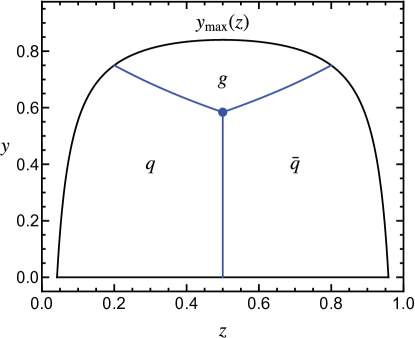
Figure 5: Phase space diagram in $(z,y)$ coordinates for two particles with equal mass (quark and anti-quark) and a massless particle (gluon). The plot is generated with the numerical value $m/Q=0.2$. The available phase space is contained between the $y=0$ and $y=y_{\rm max}(z)$ curves, which intersect at the points $(z=z_{\pm},y=0)$. Blue lines split the phase space into regions where the thrust axis points into the direction of the quark, anti-quark or gluon momenta. The three lines meet at the point $(1/2,y_{\rm middle})$, marked by a blue dot.

In this section we introduce some notation and write down the 2- and 3-body phase space in $d=4-2\varepsilon$ dimensions in terms of kinematic variables that facilitate our computation. All masses appearing in this article are understood in the pole scheme. The phase space for $n$ particles in $d=4-2\varepsilon$ dimensions is defined as

$$\int\!\mathrm{d}\Phi_{n}=(2\pi)^{d}\!\int\!\Biggl{(}\,\prod_{i=1}^{n}\frac{\mathrm{d}^{d-1}\vec{p}_{i}}{2E_{i}(2\pi)^{d-1}}\!\Biggr{)}\,\delta^{(d)}\!\biggl{(}\!P^{\mu}-\sum_{i=1}^{n}p_{i}^{\mu}\biggr{)}\,,$$ (12)

with $E_{i}=\sqrt{|\vec{p}_{i}|^{2}+m_{i}^{2}}$, since the particles are on-shell. Let us start with the $2$-body phase space for particles with the same mass $m$:

$$\Phi_{2}=(1-4\hat{m}^{2})^{\frac{1}{2}-\varepsilon}\,\Phi^{m=0}_{2}\,,\qquad\Phi^{m=0}_{2}=\frac{\Gamma(1-\varepsilon)}{2\,\Gamma(2-2\varepsilon)}\frac{Q^{-2\varepsilon}}{(4\pi)^{1-\varepsilon}}\,,$$ (13)

where, for convenience, we have factored out the $d$-dimensional $2$-body phase space for massless particles. For three particles, with particle $1$ (quark) and $2$ (anti-quark) having the same mass $m$, while particle $3$ (gluon) is massless, and adding the flux factor one obtains

$$\frac{\tilde{\mu}^{2\varepsilon}}{2Q^{2}}P(Q,\varepsilon)\int\!\mathrm{d}\Phi_{3}={} \frac{\Bigl{(}\frac{4\pi\tilde{\mu}^{2}}{Q^{2}}\Bigr{)}^{\!\varepsilon}}{256\pi^{3}\Gamma(1-\varepsilon)}\!\int\!\mathrm{d}x_{1}\,\mathrm{d}x_{2}\,\Bigl{\{}(1-x_{1})(1-x_{2})(x_{1}+x_{2}-1)$$ (14)

$$-\hat{m}^{2}(2-x_{1}-x_{2})^{2}\Bigr{\}}^{-\varepsilon}\,,$$

$$P(Q,\varepsilon)\equiv \frac{\Phi^{m=0}_{2}|_{\varepsilon\to 0}}{\Phi^{m=0}_{2}}\,,$$

with $x_{i}=2\,E_{i}/Q$, and $E_{i}$ the energy of the $i$-th particle such that energy conservation implies $x_{1}+x_{2}+x_{3}=2$. For convenience we have multiplied by the ratio of the $d=4$ and $d=4-2\varepsilon$ massless $2$-body phase-space factors. This helps taking the $\varepsilon\to 0$ limit after canceling the IR divergences. Next we implement the following variable transformation: $x_{1}=1-(1-z)\,y$, $x_{2}=1-z\,y$, such that $y=2E_{g}/Q$, which makes the soft limit $y\rightarrow 0$ manifest:

$$\frac{\tilde{\mu}^{2\varepsilon}}{2Q^{2}}P(Q,\varepsilon)\!\int\!\mathrm{d}\Phi_{3}=\frac{\Bigl{(}\frac{4\pi\tilde{\mu}^{2}}{Q^{2}}\Bigr{)}^{\!\varepsilon}}{256\pi^{3}\Gamma(1-\varepsilon)}\int\!\mathrm{d}y\,\mathrm{d}z\,y^{1-2\varepsilon}\,[\,z(1-z)(1-y)-{\hat{m}}^{2}\,]^{-\varepsilon}\,.$$ (15)

This result shows how collinear singularities, that would be located at $z=0,1$ for massless particles, are screened by the finite quark mass. In these coordinates the Dalitz region is parametrized as

$$0\leq y\leq y_{\rm max}(z)\equiv 1-\frac{\hat{m}^{2}}{z(1-z)}\,,\qquad z_{-}\leq z\leq z_{+}\,,$$ (16)

$$z_{\pm}\equiv\frac{1\pm v}{2}\,.$$

In Fig. 5 we show the phase-space boundaries for the numerical value $\hat{m}=0.2$. The phase-space limits in the $z$ variable satisfy $z_{+}z_{-}=\hat{m}^{2}$ and $z_{+}+z_{-}=1$, while the upper limit in the $y$ variable has its maximum at $y_{\rm max}(1/2)=v^{2}$. Another useful relation is given by $(z-z_{-})(z_{+}-z)=z(1-z)-\hat{m}^{2}$, a positive quantity inside the Dalitz region. In the massless limit the Dalitz plot is simply a square: $0\leq y\leq 1$, $|z|\leq 1$. The phase space (as well as all matrix elements and event-shape measurement functions) are invariant under the change $z\to 1-z$ (mirror symmetry with respect to the $z=1/2$ vertical line), since all results remain the same when exchanging quark and anti-quark.

For later use, it is convenient to split the $3$-body phase space into regions where the thrust axis points into the direction of the quark, anti-quark or gluon momenta. To that end we define

$$y_{\tau}(\hat{m},z)=\frac{\sqrt{1-4\hat{m}^{2}(1-z^{2})}-z}{1-z^{2}}\,,$$ (17)

such that these three regions are given by

$$0 \leq z\leq\frac{1}{2}\,, 0\leq y \leq y_{\tau}(\hat{m},z), {\rm quark}\,,$$

$$\frac{1}{2} \leq z\leq 1\,, 0\leq y \leq y_{\tau}(\hat{m},1-z), {\rm anti}{\text{-}}{\rm quark}\,,$$ (18)

$$0 \leq z\leq 1\,, {\rm max}\,[\,y_{\tau}(\hat{m},z),y_{\tau}(\hat{m},1-z)\,]\leq y \leq y_{\rm max}(z), {\rm gluon}\,,$$

and the lines separating the three regions meet at the point $y_{\rm middle}=4\bigl{(}\sqrt{1-3\hat{m}^{2}}-1/2\bigr{)}/3$, $z=1/2$. The quark [anti-quark] boundary meets the phase-space boundary at $z=\hat{m}$ [$z=1-\hat{m}$], $y=(1-2\hat{m})/(1-\hat{m})$.

The value of any event-shape variable for events with three particles in the final state (two quarks and a gluon) can be expressed as a function of the reduced mass $\hat{m}$ and the $z$ and $y$ phase-space variables. This function, which is not always smooth or continuous, will be referred to as the measurement function $\hat{e}(y,z)$ (for simplicity we will omit its mass dependence). Massive event-shape measurement functions $\hat{e}(z,y)$ take their minimal value if $y=0$, regardless of the value of $z$, i.e. $\hat{e}(z,0)=e_{\rm min}$, and in the soft limit $y\to 0$ the measurement function can be expanded as follows: 

$$\hat{e}(z,y)=e_{\rm min}+yf_{e}(z)+\mathcal{O}(y^{2})\equiv{\bar{e}}(y,z)+\mathcal{O}(y^{2})\,,$$ (20)

where we have defined the soft event-shape variable ${\bar{e}}$ associated to $e$, with measurement function ${\bar{e}}(y,z)=e_{\rm min}+yf_{e}(z)$. The soft event shape has the same minimal value $\bar{e}_{\rm min}=e_{\rm min}$ as the original one, but has a different maximal value, generally larger, that is attained at the highest point of the Dalitz plot, $(z,y)=(1/2,v^{2})$, as can be seen in Fig. 6:

$$\bar{e}_{\rm max}=e_{\rm min}+v^{2}f_{e}(1/2)\,.$$ (21)

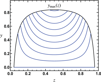
Figure 6: Phase space diagram in $(z,y)$ coordinates (black lines) showing curves with constant value of the C-parameter measurement function in the soft limit $\overline{C}$ (blue lines) with $\hat{m}=0.2$. The lines correspond to $10$ equally spaced values of $\overline{C}$ between $0$ and $0.681$. For the event shape maximal value $\overline{C}_{\rm max}=v^{2}f_{C}(1/2)$, the corresponding contour line intersects with the phase space boundary at one point only, the maximum $(1/2,v^{2})$.

3.3 Direct Computation of $\mathcal{O}(\alpha_{s})$ Results

In this approach we directly compute the differential distribution adding up real- and virtual-radiation diagrams. Our computation reproduces the few known results (either analytic or numeric), but is more general. In this approach for carrying out the calculation we explicitly show how IR singularities cancel in the sum for IR safe observables already at the differential level. We regulate them using $d=4-2\varepsilon$ dimensions (dimreg) and use plus-distribution identities to keep the computations as general and simple as possible. We have also written the $3$-body phase space in a way in which IR singularities look as close as possible to UV ones.

3.3.1 Virtual Radiation

We start with the virtual radiation diagrams, which at this order have only two particles in the final state and are common to all event shapes. The contribution to the differential cross section at $\mathcal{O}(\alpha_{s})$ comes from the interference of the tree-level and one-loop diagrams (which have IR divergences treated in dimensional regularization), and since momenta are fully constrained by energy-momentum conservation, it only contributes to the delta-function coefficient. The general form of the vector and axial-vector massive form factors up to one loop take the form 

$$V^{\mu} =\biggl{[}1+C_{F}\frac{\alpha_{s}}{\pi}A(\hat{m})\biggr{]}\gamma^{\mu}+C_{F}\frac{\alpha_{s}}{\pi}\frac{B(\hat{m})}{2m}(p_{1}-p_{2})^{\mu}\,,$$ (22)

$$A^{\mu} =\biggl{[}1+C_{F}\frac{\alpha_{s}}{\pi}C(\hat{m})\biggr{]}\gamma^{\mu}\gamma_{5}+C_{F}\frac{\alpha_{s}}{\pi}\frac{D(\hat{m})}{2m}\,\gamma_{5}\,q^{\mu}\,,$$

with $q=p_{1}+p_{2}$ the photon or Z-boson momentum, and $p_{i}$ the quark and anti-quark momenta. The vector form factor satisfies the Ward identity $q_{\mu}V^{\mu}=0$, while the longitudinal part of the axial form factor does not contribute to the cross section. Their real parts take the form Jersak:1981sp ; Harris:2001sx

$${\rm Re}[C(\hat{m})] ={\rm Re}[A(\hat{m})]+\frac{4\hat{m}^{2}}{v}L_{v}\,,$$

$${\rm Re}[D(\hat{m})] =2\,\hat{m}^{2}\biggl{[}1-\frac{2+v^{2}}{v}L_{v}\biggr{]},$$

$${\rm Re}[B(\hat{m})] =\frac{2\,\hat{m}^{2}}{v}L_{v}\,,$$ (23)

$${\rm Re}[A(\hat{m})] =\biggl{(}\frac{1+v^{2}}{2v}L_{v}-\frac{1}{2}\biggr{)}\biggl{[}\frac{1}{\varepsilon}-2\log\biggl{(}\frac{m}{\mu}\biggr{)}\biggr{]}+A_{\rm reg}(\hat{m})\,,$$

$$A_{\rm reg}(\hat{m}) =\frac{3}{2}\,v\,L_{v}-1+\,\frac{1+v^{2}}{4v}\biggl{[}\pi^{2}-2L_{v}^{2}-2\,{\rm Li}_{2}\biggl{(}\frac{2v}{1+v}\biggr{)}\biggr{]},$$

with

$$L_{v}\equiv\log\biggl{(}\frac{1+v}{2\hat{m}}\biggr{)}.$$ (24)

IR singularities look the same for both currents, and are fully contained in the transverse form factors $A$ and $C$ (note that due to current conservation the form factors are UV finite, and therefore all singularities left after carrying out the QCD renormalization program are IR). The results are singular in the $\hat{m}\to 0$ limit since collinear singularities are regulated by the finite quark mass. Furthermore in this limit the longitudinal form factors $B$ and $D$ vanish, and the transverse form factors become identical for the two currents.

The form factor contribution at $\mathcal{O}(\alpha_{s})$ is

$$\frac{1}{\sigma^{C}_{0}}\frac{\mathrm{d}\sigma^{V}_{2,\rm virt}}{\mathrm{d}e}=\frac{\alpha_{s}}{\pi}C_{F}R_{C}^{\rm virt}(\hat{m})\,\delta(e-e_{\rm min})\,,$$ (25)

$$R_{V}^{\rm virt}(\hat{m})=P(Q,\varepsilon)\,v^{1-2\varepsilon}\Bigl{\{}2\,{\rm Re}[A(\hat{m})](1+2\hat{m}^{2}-\varepsilon)-v^{2}{\rm Re}[B(\hat{m})]\Bigl{\}}$$

$$\quad\quad\quad\;\,\;=P(Q,\varepsilon)v\biggl{\{}(3-v^{2}){\rm Re}[A]-[1+2\log(v)]\biggl{(}\frac{1+v^{2}}{v}L_{v}-1\biggr{)}-v^{2}\,{\rm Re}[B]+\mathcal{O}(\varepsilon)\biggl{\}}\,,$$

$$R_{A}^{\rm virt}(\hat{m})=2\,P(Q,\varepsilon)v^{3-2\varepsilon}(1-\varepsilon)\,{\rm Re}[C(\hat{m})]$$

$$\quad\quad\;\;\,\quad=2\,P(Q,\varepsilon)v^{3}\biggl{\{}{\rm Re}[C]-[1+2\log(v)]\biggl{(}\frac{1+v^{2}}{v}L_{v}-\frac{1}{2}\biggr{)}+\mathcal{O}(\varepsilon)\biggl{\}}\,.$$

When adding these results to the real radiation contributions the $1/\varepsilon$ term present in the $A$ and $C$ form factors cancel, along with the associated $\mu$ dependence.

3.3.2 Real Radiation

Real radiation diagrams exhibit IR singularities in phase-space integrals, originating from the zero gluon-momentum limit. The matrix element squared, summed over the polarization of final-state particles and averaged over the lepton spins can be written as

$$\frac{|\sum_{\rm spin}\mathcal{M}_{C}|^{2}}{4\sigma^{C}_{0}} =\frac{256\pi^{2}\alpha_{s}\tilde{\mu}^{2\varepsilon}C_{F}}{y^{2}}M_{C}(y,z,\hat{m},\varepsilon)\,,$$ (26)

$$M_{C}(y,z,\hat{m},\varepsilon) =M^{0}_{C}(z,\hat{m})+\varepsilon M^{1}_{C}(z,\hat{m})+yM_{C}^{\rm{hard}}(y,z)+\mathcal{O}(\varepsilon^{2})\,,$$

$$M^{0}_{V}(z,\hat{m}) =-(1+2{\hat{m}}^{2})M^{1}_{V}(z,\hat{m})\,,\quad M^{1}_{V}(z,\hat{m})=-\frac{(1-z)z-\hat{m}^{2}}{(1-z)^{2}z^{2}}\,,$$

$$M^{0}_{A}(z,\hat{m}) =-M^{1}_{A}(z,\hat{m})=-v^{2}M^{1}_{V}(z,\hat{m})\,,$$

with $C=V,A$ labeling the current type and $\mu^{2}\equiv 4\pi\tilde{\mu}^{2}\mathrm{e}^{-\gamma_{E}}$. We denote the pieces which vanish for $y\to 0$ as the “hard matrix elements” $M^{\rm{hard}}_{C}$. Our results agree with those in Refs. Kramer:1979pg ; Ioffe:1978dc ; Nilles:1980ic (note that there is a known sign error in Ref. Kramer:1979pg ). The hard matrix elements can be further split as $M^{\rm{hard}}_{C}(y,z,\hat{m})=M^{2}_{C}(z,\hat{m})+yM^{3}_{C}(z,\hat{m})$, with

$$M^{2}_{C}(z,\hat{m}) =-\binom{1+2\hat{m}^{2}}{v^{2}}\frac{1}{z(1-z)}\,,$$ (27)

$$M^{3}_{C}(z,\hat{m}) =\frac{1}{2z(1-z)}\binom{1}{1+2\hat{m}^{2}}-1\,,$$

with the upper (lower) part of the expression in parentheses belonging to the vector (axial-vector) current. The radiative one-loop contribution to the differential distribution, partially expanded around $\varepsilon=0$, reads

$$\frac{1}{\sigma^{C}_{0}}\frac{\mathrm{d}\sigma^{\rm real}_{C}}{\mathrm{d}e}=$$ (28)

$$P(Q,\varepsilon)C_{F}\frac{\alpha_{s}}{\pi}\frac{\Bigl{(}\frac{4\pi\tilde{\mu}^{2}}{Q^{2}}\Bigr{)}^{\!\varepsilon}}{\Gamma(1-\varepsilon)}\int\!\frac{\mathrm{d}y\,\mathrm{d}z}{y^{1+2\varepsilon}}\,[\,z(1-z)(1-y)-{\hat{m}}^{2}\,]^{-\varepsilon}\,\delta[e-\hat{e}(y,z)]\,M_{C}(y,z,\hat{m},\varepsilon)$$

$$=P(Q,\varepsilon)C_{F}\frac{\alpha_{s}}{\pi}\biggl{\{}-\frac{\delta(e-e_{\rm min})}{2}\!\int\!\mathrm{d}z\,\biggl{[}M^{1}_{C}(z,\hat{m})+M^{0}_{C}(z,\hat{m})\biggl{(}\frac{1}{\varepsilon}+2\log\Bigl{(}\frac{\mu}{Q}\Bigr{)}$$

$$\quad-\log\bigl{[}z(1-z)-\hat{m}^{2}\bigr{]}\biggr{)}\biggr{]}+\!\int\!\mathrm{d}z\,\mathrm{d}y\,\biggl{[}M^{0}_{C}(z,\hat{m})\biggl{[}\frac{1}{y}\biggr{]}_{+}+M_{C}^{\rm{hard}}(y,z)\biggr{]}\delta[e-\hat{e}(y,z)]\biggl{\}}.$$

To get to the second line we have collected powers in $y$ and used the identity

$$y^{-1-2\varepsilon}=-\frac{1}{2\varepsilon}\delta(y)+\biggl{[}\frac{1}{y}\biggr{]}_{+}+\mathcal{O}(\varepsilon)\,,$$ (29)

in the terms containing $M^{0,1}_{C}$. The coefficient of the Dirac delta function is not yet fully explicit, as the integral over the plus function still hides singular terms. The distributional structure is completely determined in the $y\to 0$ limit, therefore we add and subtract the following term to the last integrand

$$M^{0}_{C}(z,\hat{m})\biggl{[}\frac{1}{y}\biggr{]}_{+}\delta[e-\overline{e}(y,z)]\,,$$ (30)

such that in the sum of the original and subtracted terms the plus prescription can be dropped (this can be done because the integrand goes to zero linearly with $y$). This strategy is similar to subtraction algorithms used in NLO and NNLO parton-level Monte Carlos to achieve cancellation of IR singularities between real- and virtual-radiation contributions. In our case, the subtraction helps isolating the distributional structure of the cross section. For the added term we proceed as follows

$$\int\!\mathrm{d}z\,\mathrm{d}y\,M^{0}_{C}(z,\hat{m})\biggl{[}\frac{1}{y}\biggr{]}_{+}\delta[e-\overline{e}(y,z)]\,\Theta[y_{\rm max}(z)-y]=$$

$$\int\!\mathrm{d}z\,\frac{M^{0}_{C}(z,\hat{m})}{f_{e}(z)}\biggl{[}\frac{f_{e}(z)}{e-e_{\rm min}}\biggr{]}_{+}\Theta\bigl{[}y_{\rm max}(z)-h(e,z)\bigr{]}=$$ (31)

$$-\!\delta(e-e_{\rm min})\!\int\!\mathrm{d}z\,M^{0}_{C}(z,\hat{m})\log[f_{e}(z)]+\biggl{[}\frac{1}{e-e_{\rm min}}\biggr{]}_{+}\int\!\mathrm{d}z\,M^{0}_{C}(z,\hat{m})\,\Theta\bigl{[}y_{\rm max}(z)-h(e,z)\bigr{]}\,,$$

with

$$h(e,z)\equiv\frac{e-e_{\rm min}}{f_{e}(z)}\,,$$ (32)

representing a curve in phase space defined by the condition $\bar{e}(y,z)=e$ (that is, a contour line with constant value of the soft event-shape measurement function). This line has the important property of always intersecting with the phase-space boundary $y_{\rm max}$ at two symmetric points, which will be denoted by $z_{\pm}(e)$, as shown in Fig. 7 for the C-parameter event shape. To get to the last line of Eq. (3.3.2) we have used the rescaling identity

$$\biggl{[}\frac{\log^{n}(bx)}{bx}\biggr{]}_{+}=\frac{1}{b}\biggl{\{}\frac{\log^{n+1}(b)}{n+1}\,\delta(x)+\sum_{i=0}^{n}\binom{n}{i}\log^{n-i}(b)\biggl{[}\frac{\log^{n}(x)}{x}\biggr{]}_{+}\biggr{\}}\,,$$ (33)

and the fact that if $e=e_{\rm min}$ then $h(e_{\rm min},z)=0$ and the constraint imposed by the Heaviside function $\Theta[y_{\rm max}(z)]$ is automatically satisfied [ since $y_{\rm max}(z)>0$  for $z_{-}\leq z\leq z_{+}$]. The second term in the last line of Eq. (3.3.2) is not a pure distribution yet, but can be converted to such using the relation

$$f(x)\,\biggl{[}\frac{1}{x}\biggr{]}_{+}=f(0)\,\biggl{[}\frac{1}{x}\biggr{]}_{+}+\frac{f(x)-f(0)}{x}\,.$$ (34)

Finally we arrive at

$$\int\!\mathrm{d}z\,\mathrm{d}y\,M^{0}_{C}(z,\hat{m})\,\biggl{[}\frac{1}{y}\biggr{]}_{+}\!\delta[e-\overline{e}(y,z)]=-\delta(e-e_{\rm min})\!\int\!\mathrm{d}z\,M^{0}_{C}(z,\hat{m})\log[f_{e}(z)]$$ (35)

$$+\biggl{[}\frac{1}{e-e_{\rm min}}\biggr{]}_{+}\int\!\mathrm{d}z\,M^{0}_{C}(z,\hat{m})-\!\int\!\mathrm{d}z\,M^{0}_{C}(z,\hat{m})\,\frac{\Theta[e-e_{\rm min}-y_{\rm max}(z)f_{e}(z)]}{e-e_{\rm min}}\,,$$

where we have used the identity $\Theta(x)+\Theta(-x)=1$ in the last term. The Heaviside theta function in the last integral requires $h(e,z)>y_{\rm max}(z)$, and therefore restricts the $z$ integration to the two disconnected segments shown in Fig. 7 as purple double-pointed arrows: $z_{-}\leq z\leq z_{-}(e)$ and $z_{+}(e)\leq z\leq z_{+}$, where $z_{\pm}(e)$ are the two solutions of the equation $e=\bar{e}[z,y_{\rm max}(z)]$ that lay on the original integration path $z_{-}\leq z\leq z_{+}$. The points $z_{\pm}(e)$ depend on $e$ and fulfill $z_{-}<z_{-}(e)<z_{+}(e)<z_{+}$, since $f_{e}(z)$ is positive (given that by definition $e\geq e_{\min}$) . It is useful to write the Heaviside theta in the last term as an integral over a Dirac delta function:

$$\frac{\Theta[e-e_{\rm min}-y_{\rm max}(z)f_{e}(z)]}{e-e_{\rm min}}= \int\!\mathrm{d}y\,\frac{\Theta[y-y_{\max}(z)]}{y}\,\delta[e-e_{\min}-yf_{e}(z)]\,.$$ (36)

These results provide the contribution of the real-radiation diagrams to the differential cross section shown in Eq. (1):

$$A_{e}(\hat{m})={} A_{e}^{\rm real}({\hat{m}})+R_{C}^{\rm virt}({\hat{m}})\,,$$ (37)

$$A_{e}^{\rm real}({\hat{m}})={} -\!\frac{P(Q,\varepsilon)}{2}\!\!\int\!\!\mathrm{d}z\biggl{\{}\!M^{1}_{C}(z,\hat{m})+M^{0}_{C}(z,\hat{m})\!\biggl{[}\frac{1}{\varepsilon}+2\log\Bigl{(}\frac{\mu}{Q}\Bigr{)}\!-\!\log\biggl{(}\!\frac{z(1-z)-\hat{m}^{2}}{[f_{e}(z)]^{2}}\biggr{)}\!\biggr{]}\!\biggl{\}},$$

$$B_{\rm plus}({\hat{m}})={} \!\int\!\mathrm{d}z\,M^{0}_{C}(z,\hat{m})\,,$$

$$F^{\rm NS}={} \!\int\!\mathrm{d}z\,\mathrm{d}y\,\biggl{\{}M_{C}^{\rm{hard}}(y,z)\delta[e-\hat{e}(y,z)]+\frac{M_{C}^{0}(z,\hat{m})}{y}\biggl{[}\delta[e-\hat{e}(y,z)]$$

$$-\Theta[y-y_{\max}(z)]\,\delta[e-\bar{e}(y,z)]-\delta[e-\bar{e}(y,z)]\biggr{]}\biggl{\}}\equiv F^{\rm NS}_{\rm hard}+F^{\rm NS}_{\rm soft}\,.$$

In $F^{\rm NS}$ (which can only be computed analytically for some simple event shapes), in those terms where no explicit Heaviside function is shown, a $\Theta[y_{\rm max}(z)-y]$ is understood. $F^{\rm NS}_{\rm hard}$ and $F^{\rm NS}_{\rm soft}$ correspond to the terms containing $M_{C}^{\rm hard}$ and $M^{0}_{C}$, respectively. This intermediate result already shows that the coefficient of the plus distribution is identical for all event shapes linearly sensitive to soft momentum. The non-singular term contains no distributions, and there is no singularity in the integration domain: the hard function tends linearly to zero for $y\to 0$, while the soft term contains one piece which is the difference of two delta functions with the same $y\to 0$ limit (therefore again going linearly to zero in the soft limit), and a theta function such that small values of $y$ are left out.

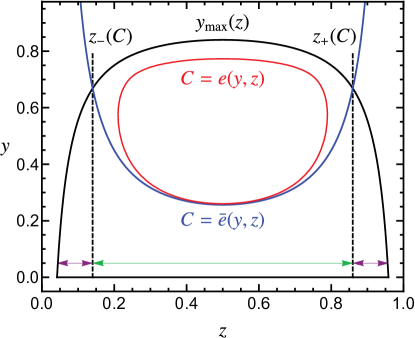
Figure 7: Phase space diagram in $(z,y)$ coordinates (black solid lines) showing a curve with constant value of the C-parameter event shape measurement function (red line) and its soft limit (blue line), using $\hat{m}=0.2$, $C=0.42$. The latter corresponds to Eq. (32), which cuts the phase-space boundary at the points $z_{\pm}(C)$. The dashed lines divide the $y=0$ axis into three segments, marked with double-pointed arrows.

3.3.3 Final Result for the Direct Computation

We first give an analytic expression for the $B_{\rm plus}$ coefficient in Eq. (37). The $z$ integration is carried out using the first line in Eq. (B), yielding

$$B_{\rm plus}(\hat{m})=\binom{3-v^{2}}{2\,v^{2}}\bigl{[}(1+v^{2})L_{v}-v\bigr{]}\,,$$ (38)

where again the first and second line of the expression in big parentheses correspond to vector and axial-vector currents, respectively. The result exhibits a log-type singularity for $m\to 0$, since in that limit the log-plus distribution associated to collinear singularities is no longer screened by the heavy quark mass.

To obtain the coefficient of the delta term we need to perform two integrals analytically, which are given in Eq. (B). Adding the results in Eqs. (25) and (37) we cancel the $1/\varepsilon$ singularity along with the $\mu$ dependence. Therefore taking the limit $\varepsilon\to 0$ amounts to setting $P(Q,\varepsilon)\to 1$, and we get

$$A^{V}_{e}(\hat{m})={} (1+2\hat{m}^{2})\biggl{\{}(1-2\hat{m}^{2})\biggl{[}{\rm Li}_{2}\biggl{(}\!-\frac{v(1+v)}{2\hat{m}^{2}}\biggr{)}-3\,{\rm Li}_{2}\biggl{(}\frac{v(1-v)}{2\hat{m}^{2}}\biggr{)}+2\log^{2}(\hat{m})+\pi^{2}$$

$$-2\log^{2}\biggl{(}\frac{1+v}{2}\biggr{)}\biggr{]}+2v\bigl{[}\log(\hat{m})-1\bigr{]}-2I_{e}(\hat{m})\biggl{\}}+(4+v^{2}-16\hat{m}^{4})L_{v}\,,$$

$$A^{A}_{e}(\hat{m})={} v^{2}\biggl{\{}(4+v^{2})L_{v}+2v\bigl{[}\log(\hat{m})-1\bigr{]}-2I_{e}(\hat{m})+(1-2\hat{m}^{2})$$ (39)

$$\times\!\biggl{[}{\rm Li}_{2}\biggl{(}\!-\frac{v(1+v)}{2\hat{m}^{2}}\biggr{)}-3\,{\rm Li}_{2}\biggl{(}\frac{v(1-v)}{2\hat{m}^{2}}\biggr{)}+\pi^{2}+2\log^{2}(\hat{m})-2\log^{2}\biggl{(}\frac{1+v}{2}\biggr{)}\biggr{]}\biggl{\}},$$

where the only event shape dependent piece is the integral

$$I_{e}(\hat{m})=\frac{1}{2}\int_{z_{-}}^{z_{+}}\!\mathrm{d}z\,\frac{(1-z)z-\hat{m}^{2}}{(1-z)^{2}z^{2}}\log[f_{e}(z)]=\int_{z_{-}}^{1/2}\!\mathrm{d}z\,\frac{(1-z)z-\hat{m}^{2}}{(1-z)^{2}z^{2}}\log[f_{e}(z)]\,,$$ (40)

where we have used the $z\leftrightarrow(1-z)$ symmetry to simplify the integration range.

4 Numerical Algorithms

Before we describe the algorithms to compute the differential and cumulative event-shape cross sections, we show how to write down the four-momenta of the three-particle phase space in terms of the $(z,y)$ coordinates. This is very useful to figure out an analytic expression for the event-shape measurement function. These expressions can in turn be used to compute the values of $e_{\rm min}$ and $e_{\rm max}$, and can be expanded around $y=0$ to obtain $f_{e}(z)$. Since we are not dealing with oriented event shapes, without any loss of generality we can choose the three particles contained in the $x-y$ plane, with the gluon 3-momenta pointing into the positive $z$ direction. With the notation $p=[E,\vec{p}\,]=[E,p_{x},p_{y},p_{z}]$ one has: 

$$p_{g} =\frac{y}{2}\,[1,0,0,1]\,,$$

$$p_{q} =\biggl{[}\frac{1-y(1-z)}{2},0,\sqrt{(1-y)(1-z)z-\hat{m}^{2}},\frac{1-y(1-z)-2z}{2}\biggr{]}\,,$$ (41)

$$p_{\bar{q}} =\biggl{[}\frac{1-yz}{2},0,-\sqrt{(1-y)(1-z)z-\hat{m}^{2}},\frac{2z-1-y\,z}{2}\biggr{]}\,.$$

The magnitude of the (anti-)quark three-momentum reads

$$|\vec{p}_{\bar{q}}|=\frac{1}{2}\sqrt{(1-y\,z)^{2}-4\hat{m}^{2}}\,,\qquad|\vec{p}_{q}|=|\vec{p}_{\bar{q}}|_{z\to 1-z}\,,$$ (42)

such that E-scheme 4-momenta are obtained by multiplying the spatial components in Eq. (4) by $E/|\vec{p}\,|$, while P-scheme 4-momenta require replacing the temporal component by $|\vec{p}\,|$, see Sec. 2. The thrust axis is simply $\hat{z}$ when pointing in the gluon direction [ see Eq. (3.2) ], while it equals $\vec{p}_{q}/|\vec{p}_{q}|$ and $\vec{p}_{\bar{q}}/|\vec{p}_{\bar{q}}|$ when pointing to the quark and anti-quark direction, respectively.

Since to compute the radiative tails of the distributions (either differential or cumulative) and the moments of the differential distributions one only needs the real radiation contribution, in this section we adopt the shorthand notation

$$M_{C}(y,z)\equiv M_{C}(y,z,\hat{m},\varepsilon=0)\,.$$ (43)

4.1 Computation of Moments

An especially convenient way to compute the $n$ -th moment of the distribution is expressing it in terms of the total hadronic cross section and displaced moments:

$$\langle(e-e_{\min})^{n}\rangle\equiv\frac{1}{\sigma^{C}_{0}}\!\int^{e_{\max}}_{e_{\min}}\!\mathrm{d}e\,(e-e_{\min})^{n}\frac{\mathrm{d}\sigma}{\mathrm{d}e}\,,\qquad\langle(e-e_{\min})^{0}\rangle=R(\hat{m})\,.$$ (44)

The reduced moments at $\mathcal{O}(\alpha_{s})$ and for $n>0$ can be computed directly using a numerical 2D integration, which is convergent due to the insertion of the displaced measurement function

$$\langle(e-e_{\min})^{n}\rangle=C_{F}\frac{\alpha_{s}}{\pi}\!\int\!\mathrm{d}y\,\mathrm{d}z\,[\,\hat{e}(y,z)-e_{\min}\,]^{n}\,\frac{M_{C}(y,z)}{y}+\mathcal{O}(\alpha_{s}^{2})\,.$$ (45)

The integration can be carried out with a MC procedure, but it is faster and more efficient to use a deterministic integrator in 2D. For our numerical checks we have used the dblquad routine included in the scipy.integrate Virtanen:2019joe python module. Finally, an efficient way of numerically computing regular moments is

$$\langle e\rangle^{n}=e^{n}_{\rm min}\,R(\hat{m})+C_{F}\frac{\alpha_{s}}{\pi}\!\int\!\mathrm{d}y\,\mathrm{d}z\,[\hat{e}(y,z)^{n}-e^{n}_{\rm min}]\,\frac{M_{C}(y,z)}{y}+\mathcal{O}(\alpha_{s}^{2})\,,$$ (46)

such that the numerical integral is convergent and can be directly computed in a standard way.

4.2 Computation of Cross Sections Using a MC

Before we describe our novel numerical algorithm to directly compute the differential and cumulative cross sections, we briefly review how this is done using MC methods. The MC can only access the radiative tail of the distribution, and therefore one needs to consider only real radiation diagrams. To obtain the differential distribution one needs to integrate over a Dirac delta function of the event-shape measurement function. Since there is no known way of doing this in the MC approach, one instead bins the distribution, such that the delta gets replaced by the difference of Heaviside functions. More specifically, by integrating first over the event-shape bin we obtain

$$\Sigma(e_{2})-\Sigma(e_{1})=\!\int\!\frac{\mathrm{d}y\,\mathrm{d}z}{y}\,\mathrm{d}e\,\delta[e-\hat{e}(y,z)]M_{C}(y,z)\,\Theta(e-e_{1})\,\Theta(e_{2}-e)=$$ (47)

$$\int\!\frac{\mathrm{d}y\,\mathrm{d}z}{y}\,\Theta[\hat{e}(y,z)-e_{1}]\,\Theta[e_{2}-\hat{e}(y,z)]M_{C}(y,z)\,.$$

The advantage of the MC method is that one can compute the binned distribution for all event shapes in a single run. In practice one chooses a set of bins for each event-shape variable ahead of time. In our implementation of the MC algorithm, we match the $(y,z)$ phase space into the unit square with the following change of variables:

$$y=v^{2}\,t_{1}\,,\qquad z=\frac{1}{2}+\Bigl{(}t_{2}-\frac{1}{2}\Bigr{)}\sqrt{1-\frac{4\hat{m}^{2}}{1-y}}\,,$$ (48)

$$\mathrm{d}y\,\mathrm{d}z=v^{2}\sqrt{1-\frac{4\hat{m}^{2}}{1-y}}\,\mathrm{d}t_{1}\,\mathrm{d}t_{2}\,.$$

Now Eq. (47) has a nice interpretation in terms of MC’s: a) generate a sample of points in the $(t_{1},t_{2})$ unit square, compute for each one of them $(y,z)$ and from that get numerical values for all event-shape variables, matrix elements and the Jacobian; b) for each random point and for every event shape, figure out which bin it corresponds to; c) add the numerical values of the matrix element (times Jacobian) for each bin; d) normalize each bin to the total number of points in the random sample. Statistical uncertainties can be obtained in the usual way, and several independent runs can be combined. The method can of course be refined using importance sampling, and in our numerical code we use the python implementation of VEGAS Lepage:1980dq . The advantage of the MC is that a single run can be used to compute the full distribution for all event shapes at once, and even to compute other quantities such as moments of the distribution or the cumulative cross-section.

4.3 Direct Computation of the Differential Cross Section

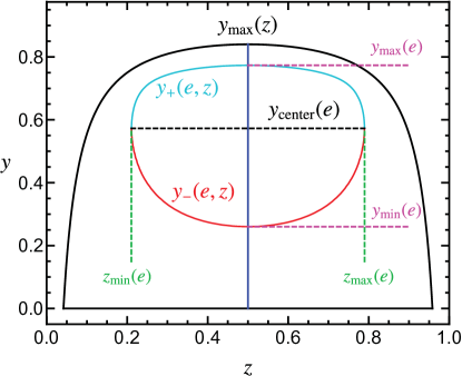
Figure 8: Phase space diagram in $(z,y)$ coordinates (black lines) showing in red and cyan the contour line with constant value of C-parameter, corresponding to the functions $y_{+}(e,z)$ and $y_{-}(e,z)$, respectively. The two curves meet at the points $[z_{\min,\max}(e),y_{\rm center}(e)]$, joined by the black, dashed line. These curves meet the $z=1/2$ vertical blue line for $y=y_{\min,\max}(e)$, respectively. Dashed magenta [green] lines mark the points of maximal and minimal values that $y$ [$z$] can take within the red curve. To generate this plot the values $\hat{m}=0.2$ and $C=0.42$ were used.

In this section we describe an alternative method which does not have the limitations inherent to a MC (can only compute binned cross sections, and in general one needs to specify the bins ahead of time). The direct method computes directly the (unbinned) differential cross section, and since it only uses “deterministic” integration methods, it can in principle achieve arbitrary precision in very small run-time. The only requirement for the method to be applicable is that one can compute the value of the event shape and its first derivative in terms of the phase-space variables $y$ and $z$. On the other hand, as compared to the MC method, one needs to compute a numerical integral for each current, each event shape and each point in the spectrum. We denote the radiative tail of the distribution by $F_{e}(e,\hat{m})$, defined as

$$F_{e}(e,\hat{m})\equiv\frac{B_{\rm plus}({\hat{m}})}{e-e_{\rm min}}+F_{e}^{\rm NS}(e,\hat{m})\,.$$ (49)

Since we can compute $F_{e}$ numerically with high precision and the values of $B_{\rm plus}$ and $e_{\rm min}$ are known analytically, $F_{e}^{\rm NS}$ can be readily obtained. This is the last ingredient for the full description of the $\mathcal{O}(\alpha_{s})$ differential cross section. It should be noted that even in the massless limit $F_{e}(e,0)$ is not always analytically known (e.g. for angularities or broadening). On the other hand, in the $m\to 1/2$ limit $F_{e}(e,1/2)=0$ and only singular terms survive, which are analytically computed in Sec. 3.

Let us first discuss how to obtain the cross section for a toy model: an event shape whose measurement function coincides with the soft limit of some regular event shape. We proceed by integrating the $y$ variable analytically, followed by a numerical integration of the $z$ variable. The $z$ integration boundaries are set by $z_{\pm}(e)$, the intersection of $h(e,z)$ with $y_{\rm max}(z)$, see Fig. 7. Therefore we get

$$\frac{1}{\sigma^{C}_{0}}\frac{\mathrm{d}\sigma_{C}}{\mathrm{d}\bar{e}} =C_{F}\frac{\alpha_{s}}{\pi}\!\int\!\mathrm{d}y\,\mathrm{d}z\,\frac{M_{C}(y,z)}{y}\,\delta[\bar{e}-e_{\rm min}-yf_{e}(z)]$$ (50)

$$=\frac{C_{F}}{\bar{e}-e_{\rm min}}\frac{\alpha_{s}}{\pi}\!\int_{z_{-}(e)}^{z_{+}(e)}\!\mathrm{d}z\,M_{C}\biggl{(}\frac{\bar{e}-e_{\rm min}}{f_{e}(z)},z\biggr{)}\,.$$

To illustrate how the method works for “real” event shapes, let us assume for now that we are dealing with an observable such that contour lines with constant event-shape value (that is, that the curve defined by the condition $\hat{e}(y,z)=e$ for some value of $e$ satisfying $e_{\rm min}<e<e_{\rm max}$) is continuous, convex and does not intersect with the phase-space boundary (the method can be adapted for observables not satisfying this criteria, as will be explained later). Every event shape we considered, except for 2-jettiness, C-jettiness and HJM (that intersect with the phase-space boundaries for some values of $e$), and E-scheme variables other than C-parameter (that are not continuous) satisfy this condition. Curves for all event shapes which use the thrust axis have kinks, but this does not pose a problem for the method. We proceed by integrating $y$ with the Dirac delta function first, while the $z$ integral is performed numerically afterwards. The first step is finding the maximal and minimal value of $y$ in the contour line of constant event-shape value, which we call $y_{\rm max}(e)$ and $y_{\rm min}(e)$, respectively. Since the curve is convex and symmetric under $z\to 1-z$, these two values are attained for $z=1/2$. To find them, one has to solve the equation

$$\hat{e}\Bigl{(}y,\frac{1}{2}\Bigr{)}=e\,,$$ (51)

which can be done e.g. with the Brent algorithm brent2002algorithms . In our numerical code we use the function brentq from the scipy.optimize python module. The two roots are easily found since $y_{\rm min}$ is between $0$ and $y_{\rm middle}$, while $y_{\rm max}$ is between $y_{\rm middle}$ and $v=\sqrt{1-4\hat{m}^{2}}$, with $(0.5,y_{\rm middle})$ being the point at which the lines that divide the phase space into regions with the thrust axis pointing to the quark, anti-quark, or gluon $3$-momentum coincide: 

$$y_{\rm middle}=\frac{4}{3}\biggl{(}\!\sqrt{1-3\hat{m}^{2}}-\frac{1}{2}\biggr{)}\,.$$ (52)

In the second step we obtain the contour lines of constant $e$ parametrized as two functions of $y$. This is obtained by solving the equation $\hat{e}(y,z)=e$ for $z$ at a given value of $y$. There are two solutions to this equation, which we call $z_{\pm}(e,y)$, but we will numerically obtain only $z_{-}(e,y)<1/2$, since the other solution can be obtained by symmetry. Again, we employ the Brent algorithm, since we know the solution is always contained between $z=1/2$ and the phase-space boundary $z_{-}^{\rm border}(y)$, which as a function of $y$ is written as

$$z_{\pm}^{\rm border}(y)=\frac{1}{2}\Biggl{(}1\pm\sqrt{\frac{1-y-4\hat{m}^{2}}{1-y}}\;\Biggr{)}\,.$$ (53)

In our numerical code we again use the brentq function. Since we compute the distribution solving the Dirac delta function in terms of the variable $y$, the next step is figuring out the lower integration limit in the $z$ variable, dubbed $z_{\rm min}(e)$. Since the integrand is symmetric around $z=1/2$, we will integrate in the range $z=[\,z_{\rm min}(e),1/2]$ and double the result. The value of the point with the smallest $z$ value for a given event-shape value $e$, $[\,z_{\rm min}(e),y_{\rm center}(e)\,]$, is obtained numerically as the minimum of the function $z_{-}(e,y)$. The minimum lies between the values $y_{\rm max}(e)$ and $y_{\rm min}(e)$ previously determined, and we use the Brent algorithm implemented in the minimize_scalar function from the scipy.optimize python module, which finds the minimum in a given interval. The maximum event shape value $e_{\rm max}$ satisfies $z_{\rm min}(e_{\rm max})=z_{\rm max}(e_{\rm max})=1/2$. The last ingredient we need to determine before performing the numerical integral in $z$ is the contour line of constant $e$ as a function of $z$. It is obtained by solving the equation $\hat{e}(y,z)=e$ for $y$ at a given value of $z$, which has two solutions which we denote by $y_{\pm}(e,z)$, corresponding to the two zeroes of the Dirac delta function argument when integrating the $y$ variable. The lower and upper solutions are contained in the intervals $[\,y_{\rm min}(e),y_{\rm center}(e)\,]$ and $[\,y_{\rm center}(e),y_{\rm max}(e)\,]$, respectively, and are easily found numerically, once again employing the Brent algorithm already described. In Fig. 8 we show graphically the position of $z_{\min,\max}(e)$, $y_{\rm center}(e)$ and $y_{\min,\max}(e)$, as well as the curves $y_{\pm}(e,z)$, while Fig. 9 shows the $z_{\pm}^{\rm border}(z)$ and $z_{\pm}(e,z)$ lines. Putting everything together, the differential distribution can be written as 

$$F_{e}(e,\hat{m})=\!\int\!\mathrm{d}z\,\mathrm{d}y\,\frac{M_{C}(y,z)}{y}\,\delta[e-\hat{e}(y,z)]=2\!\int_{z_{\rm min}(e)}^{1/2}\!\mathrm{d}z\sum_{y=y_{\pm}(e,z)}\frac{M_{C}(y,z)}{y\,\Big{|}\frac{\mathrm{d}\hat{e}(y,z)}{\mathrm{d}y}\Big{|}}\,,$$ (55)

where the sum in $y$ means that we evaluate the $y$-dependent expression for both $y=y_{\pm}(e,z)$ and add the results. The derivative of the event-shape measurement function with respect to $y$ is performed analytically, while the value of $y_{\pm}(e,z)$ is obtained numerically with the procedure outlined above. Our code computes the numerical integral using the python quad function, which is the quadpack RobertPiessensQasp package implementation of the scipy.integrate module.

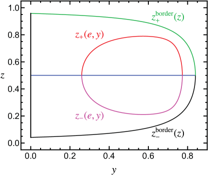
Figure 9: Phase space diagram in $(y,z)$ coordinates depicted as green and black lines, corresponding to the functions $z_{+}^{\rm border}(z)$ and $z_{-}^{\rm border}(z)$, respectively. The red and magenta lines show a contour line with constant value of C-parameter, corresponding to the functions $z_{+}(e,y)$ and $z_{-}(e,y)$, respectively. To generate this plot the numerical values $\hat{m}=0.2$ and $C=0.42$ were used.

We close the section explaining how to modify the algorithm to compute E-scheme thrust, broadening and HJM. The contour lines for these event shapes never intersect with the phase-space boundaries (at most they are tangent to it at a single point), but are not always continuous. It turns out that if $\tau^{E}<\hat{m}$, $B^{E}<\hat{m}/2$ or $\rho^{E}<\hat{m}(1-2\hat{m})/(1-\hat{m})$, the event-shape contour lines are continuous and convex, such that the algorithm described above can be used. For larger values, the lines of constant event-shape value show discontinuities exactly along the lines that delimit the regions with the thrust axis pointing in the gluon or (anti-)quark direction. Therefore we find it convenient to define event-shape measurement functions in each of the three regions: $\hat{e}_{q}(y,z)$, $\hat{e}_{\bar{q}}(y,z)$ and $\hat{e}_{g}(y,z)$. It is clear that one should first determine the intersection points of the contour lines in the quark and gluon regions with $y_{\tau}(\hat{m},z)$, defined in Eq. (3.2), which we call $z_{\pm}^{q}(e)$ and $z_{\pm}^{g}(e)$, with $z_{+}^{q,g}(e)=1-z_{-}^{q,g}$. We find that in all cases $z_{-}^{g}(e)>z_{-}^{q}(e)$. These points are computed solving the equations $\hat{e}_{q}[\,y_{\tau}(\hat{m},z),z\,]=e$ and $\hat{e}_{g}[\,y_{\tau}(\hat{m},z),z\,]=e$ for $z$. In our code we employ the Brent algorithm again, and use that the solutions are to be found in the interval $z\in[\hat{m},1/2]$.

For E-scheme thrust and HJM one only needs to compute $y_{-}(e,z)$ and $y_{+}(e,z)$, which now coincide with the contours in the quark and gluon regions, respectively. Therefore the equations to solve are $\hat{e}_{q}(y,z)=e$ and $\hat{e}_{g}(y,z)=e$, for which we use the Brent algorithm, and use the fact that the solutions have to be contained in the ranges $y\in[\,0,y_{\tau}(\hat{m},z)\,]$ and $y\in[\,y_{\tau}(\hat{m},z),y_{\rm max}(z)\,]$, respectively. In Fig. 10, for $\tau^{E}=0.27$ we show the functions $y_{\pm}(e,z)$ in red and blue, as well as the points $z_{\pm}^{q}(e)$ and $z_{\pm}^{g}(e)$ with dashed black lines. The cross section then is computed as

$$F_{e}(e,\hat{m})=2\!\int_{z_{-}^{q}(e)}^{1/2}\!\mathrm{d}z\,\Biggl{|}\frac{M_{C}(y,z)}{y\,\frac{\mathrm{d}\hat{e}(y,z)}{\mathrm{d}y}}\Biggr{|}_{y=y_{-}(e,z)}+2\!\int_{z_{-}^{g}(e)}^{1/2}\!\mathrm{d}z\,\Biggl{|}\frac{M_{C}(y,z)}{y\,\frac{\mathrm{d}\hat{e}(y,z)}{\mathrm{d}y}}\Biggr{|}_{y=y_{+}(e,z)}\,.$$ (56)

The most involved event shape is E-scheme broadening, which requires a specific algorithm. For $B_{T}^{E}>\hat{m}/2$ but smaller than a certain critical value $B_{T}^{E,\rm crit}$, and for the small range $z\in[\,z_{\rm min}(e),z_{-}^{q}(e)\,]$, there are two solutions to the equation $\hat{e}_{q}(y,z)=e$, which we call $y_{-}(e,z)$ and $y_{\rm up}(e,z)$. The value of $z_{\rm min}(e)$ is computed using the algorithm already explained for continuous event shapes, and the values of $z_{-}^{q,g}(e)$ are computed as described in the previous paragraph. In Fig. 11 we show the functions $y_{\pm}(e,z)$ and $y_{\rm up}(e,z)$ in green, red and cyan, respectively. The points $z_{\rm min}(e)$ and $z_{-}^{q,g}(e)$ are marked with black, dashed lines. Therefore, while for $B_{T}>B_{T}^{E,\rm crit}$, one simply uses Eq. (56), if $\hat{m}/2<B_{T}^{E}<B_{T}^{E,\rm crit}$ the following expression has to be employed:

$$F_{e}(e,\hat{m})\,={} 2\!\int_{z_{\rm min}(e)}^{z_{-}^{q}(e)}\!\mathrm{d}z\sum_{y=y_{-}(e,z)}^{y_{\rm up}(e,z)}\frac{M_{C}(y,z)}{y\,\Big{|}\frac{\mathrm{d}\hat{e}(y,z)}{\mathrm{d}y}\Big{|}}+2\!\int_{z_{-}^{q}(e)}^{1/2}\!\mathrm{d}z\,\Biggl{|}\frac{M_{C}(y,z)}{y\,\frac{\mathrm{d}\hat{e}(y,z)}{\mathrm{d}y}}\Biggr{|}_{y=y_{-}(e,z)}$$ (57)

$$+2\!\int_{z_{-}^{g}(e)}^{1/2}\!\mathrm{d}z\,\Biggl{|}\frac{M_{C}(y,z)}{y\,\frac{\mathrm{d}\hat{e}(y,z)}{\mathrm{d}y}}\Biggr{|}_{y=y_{+}(e,z)}\,.$$

For $e$ larger than a certain value $e_{\rm th}$, the contour lines for thrust, HJM and broadening in the E-scheme exist only in the gluon region, or in other words, $z_{\pm}^{q}(e_{\rm th})=1/2$, such that only the second term in Eq. (56) contributes. $e_{\rm max}$ obviously satisfies $z_{\pm}^{g}(e_{\rm max})=1/2$. Some results for differential and cumulative distributions of 2-jettiness, C-jettiness and HJM will be discussed in Sec. 5.

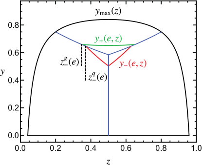
Figure 10: Phase-space diagram in $(z,y)$ coordinates (black curves) split by blue lines into regions in which the thrust axis points in the direction of the quark, anti-quark or gluon momenta. In green and red we show the contour lines for constant value of $\tau^{E}$ corresponding to the functions $y_{+}(e,z)$ and $y_{-}(e,z)$, respectively. The two curves do not meet at any point, but intersect with the boundary separating the gluon and quark regions at the points $z_{-}^{q}(e)$ and $z_{-}^{g}(e)$, marked with dashed black lines. To generate this plot the parameters $\hat{m}=0.2$ and $\tau^{E}=0.27$ were used.

4.4 Computation of the Cumulative Distribution

We define the cumulative distribution as

$$\Sigma(e_{c})=\frac{1}{\sigma_{0}}\!\int_{0}^{e_{c}}\!\mathrm{d}e\,\frac{\mathrm{d}\sigma}{\mathrm{d}e}=R_{0}(\hat{m})\,\Theta(e_{c}-e_{\rm min})+C_{F}\frac{\alpha_{s}}{\pi}\,\Sigma^{1}(e_{c})+\mathcal{O}(\alpha_{s}^{2})\,.$$ (58)

Once again, since we can compute $\Sigma^{1}(e_{c})$ with very high precision, the non-singular $\Sigma^{\rm NS}(e_{c})$ function can be obtained by removing the contributions from the delta and plus functions, which are known analytically. This is the last ingredient for the complete description of the cumulative cross section at $\mathcal{O}(\alpha_{s})$.

The cumulative distribution provides an alternative, numeric way of computing the delta coefficient, that will be used as an additional cross check of our computation in Sec. 4 (see Appendix A)

$$A_{e}(\hat{m})=\lim_{e_{c}\to e_{\rm min}}\Sigma^{1}(e_{c})-B_{\rm plus}(\hat{m})\log(e_{c}-e_{\rm min})\,.$$ (59)

In practice one can compute the one-loop contribution to the cumulative distribution by adding and subtracting the total hadronic cross section $R_{1}^{C}(\hat{m})=\Sigma^{1}_{C}(e_{\max})$, and then using $1-\Theta(x)=\Theta(-x)$, to obtain the relation

$$\Sigma^{1}_{C}(e_{c})=R_{1}^{C}(\hat{m})+\Sigma^{1}_{C}(e_{c})-\Sigma^{1}_{C}(e_{\max})=R_{1}^{C}(\hat{m})-\!\int\!\mathrm{d}y\,\mathrm{d}z\,\Theta[\hat{e}(y,z)-e_{c}]\,\frac{M_{C}(y,z)}{y}\,.$$ (60)

The functions $R_{1}^{C}$ are shown graphically in Fig. 4. The cancellation of IR singularities is already realized in $R_{1}^{C}$ and the integral left over involves only real radiation. Since the Heaviside function limits the $y$ integration on the lower side, the integral is convergent, and consequently can be carried out using standard methods. For instance, the MC method described in Sec. 4.2 can be easily adapted by simply summing up the events of all bins with lower endpoint larger larger than $e_{c}$.

In the rest of this section we describe a direct method along the lines of Sec. 4.3. We again start with our toy model, namely the event shape defined as the soft limit of another variable:

$$\Sigma^{1}_{C}(\bar{e}_{c}) =R_{1}^{C}(\hat{m})-\!\int_{z_{-}(\bar{e}_{c})}^{z_{+}(\bar{e}_{c})}\!\mathrm{d}z\int_{h(\bar{e}_{c},z)}^{y_{\rm max}(z)}\mathrm{d}y\,\frac{M_{C}(y,z)}{y}$$ (61)

$$=R_{1}^{C}(\hat{m})-\!\int_{z_{-}(\bar{e}_{c})}^{z_{+}(\bar{e}_{c})}\!\mathrm{d}z\,\mathcal{M}_{C}[\,y_{\rm max}(z),h(\bar{e}_{c},z),z,\hat{m}]\,,$$

where, given that the matrix element is a rank-two polynomial in $y$, the innermost integration can be performed analytically

$$\!\int_{y_{1}}^{y_{2}}\!\mathrm{d}y\,\frac{M_{C}(y,z)}{y}\equiv{} \mathcal{M}_{C}(y_{1},y_{2},z,\hat{m})=M_{C}^{0}(z,\hat{m})\log\biggl{(}\frac{y_{1}}{y_{2}}\biggr{)}$$ (62)

$$+M_{C}^{2}(z,\hat{m})\,(y_{1}-y_{2})+\frac{1}{2}M_{C}^{3}(z,\hat{m})\,(y_{1}^{2}-y_{2}^{2})\,.$$

The logarithm multiplying $M_{C}^{0}$ reflects the soft singularity and diverges if $\bar{e}_{c}=e_{\rm min}$. The $z$ integration in Eq. (61) can be easily performed numerically, and it corresponds to the area marked with II in Fig. 21. 

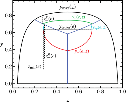
Figure 11: Phase space diagram in $(z,y)$ coordinates (black curves) split by blue lines into regions in which the thrust axis points in the direction of the quark, anti-quark or gluon momenta. In green, cyan and red we show the contour lines for constant value of $\tau^{E}$ corresponding to the functions $y_{+}(e,z)$, $y_{\rm up}(e,z)$ and $y_{-}(e,z)$, respectively. The cyan and green curves do not meet at any point, but intersect with the boundary separating the gluon and quark regions at the points $z_{-}^{q}(e)$ and $z_{-}^{g}(e)$, marked with dashed black lines. The cyan and red curves meet at the points $[\,z_{\min,\max}^{q}(e),y_{\rm center}(e)]$. To generate this plot the values $\hat{m}=0.2$ and $B_{T}^{E}=0.2$ were used.

For regular event shapes whose contour lines for constant $e$ are continuous, convex and do not intersect with the phase-space boundaries, the cumulative distribution can be computed easily using the ingredients described in Sec. 3.3:

$$\Sigma^{1}_{C}(\bar{e}_{c})=R_{1}^{C}(\hat{m})-2\!\int_{z_{\rm min}(e)}^{1/2}\!\mathrm{d}z\,\mathcal{M}_{C}[\,y_{+}(e,z),y_{-}(e,z),z,\hat{m}]\,.$$ (63)

The $z$ integration is performed numerically as described in Sec. 3.3. We have checked that taking a numerical derivative of our cumulative distribution reproduces the differential cross section as computed in the previous section.

For E-scheme thrust and HJM the above formula has to be modified. From the analysis in the previous section and looking at Fig. 10, one can readily conclude that between $z_{-}^{g}(e)$ and $z_{-}^{q}(e)$ the area to be integrated is limited by $y_{\tau}(\hat{m},z)$ and $y_{+}(e,z)$, while between between $z_{-}^{q}(e)$ and $1/2$ it is limited by $y_{-}(e,z)$ and $y_{+}(e,z)$:

$$\Sigma^{1}_{C}(\bar{e}_{c})={} R_{1}^{C}(\hat{m})-2\!\int_{z_{-}^{g}(e)}^{z_{-}^{q}(e)}\!\mathrm{d}z\,\mathcal{M}_{C}[\,y_{+}(e,z),y_{\tau}(\hat{m},z),z,\hat{m}]$$ (64)

$$-2\!\int_{z_{-}^{q}(e)}^{1/2}\!\mathrm{d}z\,\mathcal{M}_{C}[\,y_{+}(e,z),y_{-}(e,z),z,\hat{m}]\,.$$

Finally, for E-scheme broadening, if $\hat{m}/2<B_{T}^{E}<B_{T}^{E,\rm crit}$ one has to use the following expression:

$$\Sigma^{1}_{C}(\bar{e}_{c})={} R_{1}^{C}(\hat{m})-2\!\int_{z_{\rm min}(e)}^{z_{-}^{q}(e)}\!\mathrm{d}z\,\mathcal{M}_{C}[\,y_{\rm up}(e,z),y_{-}(e,z),z,\hat{m}]$$

$$-2\!\int_{z_{-}^{g}(e)}^{z_{-}^{q}(e)}\!\mathrm{d}z\,\mathcal{M}_{C}[\,y_{+}(e,z),y_{\tau}(\hat{m},z),z,\hat{m}]$$ (65)

$$-2\!\int_{z_{-}^{q}(e)}^{1/2}\!\mathrm{d}z\,\mathcal{M}_{C}[\,y_{+}(e,z),y_{-}(e,z),z,\hat{m}]\,.$$

All the $z$ numerical integrals in this section are performed using the python quadpack implementation in the scipy module.

The cumulative distribution for event shapes whose contour lines intersect with the phase space will be discussed in the next section taking 2-jettiness as an example.

5 Cross Sections for Mass-Sensitive Event Shapes

As an application of the approach presented in this work, we now work out differential and cumulative cross sections for those event shapes whose contour lines intersect with the phase-space boundaries: HJM, 2-jettiness and C-jettiness. These happen to be the most sensitive to the heavy quark mass, since their threshold gets displaced from zero to a mass-dependent position. Analytic results for the differential 2-jettiness Dehnadi:2016snl and C-jettiness distributions Preisser:mthesis   are already known, but in this section we will carry out the manipulations necessary to bring their computation into 1D integrals over $z$. We shall show how to obtain analytical results for the differential heavy jet mass and cumulative 2-jettiness distributions. Since the coefficients of the delta functions are already collected in Appendix D and the plus-distribution coefficient is universal, the only missing piece is the non-singular contribution, which can be computed in $d=4$ dimensions.

5.1 Differential HJM

In order to derive the HJM differential distribution it is useful to split the phase space into the usual three regions, as described by Eq. (3.2) and shown in Fig. 5. For three particles, one of them massless and the other two with same mass $m$, $\rho(y,z)$ takes the following form in these regions: 

$$\rho_{q}=\hat{m}^{2}+yz\,,\qquad\rho_{\bar{q}}=\hat{m}^{2}+y(1-z)\,,\qquad\rho_{g}=1-y\,.$$ (66)

Consequently, the measurement delta functions in the respective regions are very simple and given by

$$\delta(\rho-yz-\hat{m}^{2})=\frac{1}{z}\delta\biggl{(}y-\frac{\rho-\hat{m}^{2}}{z}\biggr{)}\,, \qquad\delta[\rho-y(1-z)-\hat{m}^{2}]=\frac{1}{1-z}\delta\biggl{(}y-\frac{\rho-\hat{m}^{2}}{1-z}\biggr{)}\,,$$

$$\delta(\rho-1+y)\,.$$ (67)

To figure out the correct integration boundaries for $y$ and $z$ we consider the quark and anti-quark region first. In this region, the lines of constant $\rho$ meet either the phase-space boundary [ for $\rho<\hat{m}(1-\hat{m}-\hat{m}^{2})/(1-\hat{m})$ ], or the boundary to the gluon region (for larger values). Defining $\xi_{\rho}\equiv\sqrt{t_{\rho}^{2}-4\rho}$ and $t_{\rho}=1+\rho-\hat{m}^{2}$, the intersections with the phase-space boundary are located at $z=z_{1}\equiv(t-\xi_{\rho})/2$ and $z=1-z_{1}$, while the intersections with the gluon-region boundary are located at $z=z_{2}\equiv(t_{\rho}-1)/\sqrt{(1-\rho)^{2}-2\hat{m}^{2}(1+\rho)+\hat{m}^{4}}$ and $z=1-z_{2}$. The gluon region, on the other hand, contributes only for $\rho>4\hat{m}^{2}$, intersecting the phase-space boundary [ for $\rho<\hat{m}/(1-\hat{m})$ ] or the region boundary (for larger values). The phase-space boundary intersections are located at $z=z^{2}_{-}\equiv\bigl{[}\,1-\sqrt{1-4\hat{m}^{2}/\rho}\;\bigr{]}/2$ and $z=z^{2}_{+}\equiv 1-z^{2}_{-}$ for $\rho<\hat{m}/(1-\hat{m})$, while the region boundary intersections are located at $z=z^{3}_{-}\equiv\bigl{[}\,1-\sqrt{(1-\rho^{2})+4\hat{m}^{2}}\;\bigr{]}/(1-\rho)$ and $z=z^{3}_{+}\equiv 1-z^{3}_{-}$. All those cases are shown in Fig. 12.

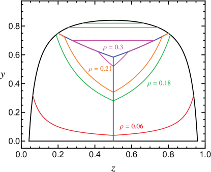
Figure 12: Three-particle phase space (black lines), thrust boundaries (blue lines) and constant $\rho$ value contour lines, with $\hat{m}=0.2$.

Note that that the constant event-shape lines of the (anti-)quark and the gluon region do not meet at the region boundaries.

Taking all this into account, the differential cross section in $d=4$ is given by

$$F_{\rho}(\rho,\hat{m})={} 2\!\int^{\frac{1}{2}}_{\max(z_{1},z_{2})}\frac{\text{d}z}{\rho-\hat{m}^{2}}M_{C}\biggl{(}\frac{\rho-\hat{m}^{2}}{z},z\biggr{)}+\frac{2\,\Theta(\rho-4\hat{m}^{2})}{1-\rho}\!\int^{\frac{1}{2}}_{\max(z^{2}_{-},z^{3}_{-})}\!\!\text{d}z\,M_{C}(1-\rho,z)$$

$$={} f_{1}[\max(z_{1},z_{2})]+f_{2}[\max(z^{2}_{-},z^{3}_{-})]\,,$$ (68)

with the integral solutions

$$f^{V}_{1}(z)={} \frac{(1-2z)\bigl{[}\,\rho(1-z)(\rho-4z)-2\hat{m}^{2}(\rho+2(1-2\rho)z^{2}+3\rho z)+\hat{m}^{4}(1-z-8z^{2})\,\bigr{]}}{2(1-z)z^{2}(\rho-\hat{m}^{2})}$$

$$+\biggl{(}\rho-2-5\hat{m}^{2}+2\frac{1-4\hat{m}^{4}}{\rho-\hat{m}^{2}}\biggr{)}\log\biggl{(}\frac{1-z}{z}\biggr{)}\,,$$

$$f^{A}_{1}(z)={} 4-8\hat{m}^{2}(2+\rho)+8\hat{m}^{4}+\frac{1}{2(\rho-\hat{m}^{2})}\biggl{\{}\frac{(1+2\hat{m}^{2})(\rho-\hat{m}^{2})^{2}}{z^{2}}+\frac{4(1-4\hat{m}^{2})\hat{m}^{2}}{1-z}$$

$$-2\,\frac{\rho(2+\rho)-2\hat{m}^{2}\rho(5+\rho)+\hat{m}^{4}(1+4\rho)-2\hat{m}^{6}}{z}$$

$$+2\bigl{[}\,2-(2-\rho)\rho+2\hat{m}^{2}(\rho(\rho+3)-5)+\hat{m}^{4}(9-4\rho)+2\hat{m}^{6}\bigr{]}\log\biggl{(}\frac{1-z}{z}\biggr{)}\biggl{\}}\,,$$

$$f^{V}_{2}(z)={} \frac{1}{t}\biggl{\{}[2-(2-t)t-4\hat{m}^{2}t-8\hat{m}^{4}]\log\biggl{(}\frac{1}{z}-1\biggr{)}-\frac{(1-2z)\bigl{[}(1-z)z\,t^{2}+2\hat{m}^{2}+4\hat{m}^{4}\bigr{]}}{(1-z)z}\biggl{\}}\,,$$

$$f^{A}_{2}(z)={} \frac{\bigl{[}2-2t+t^{2}+2\hat{m}^{2}(t^{2}+4t-6)+16\hat{m}^{4}\bigr{]}\log\biggl{(}\frac{1}{z}-1\biggr{)}-\frac{(1-2z)[t^{2}(1-z)z+2\hat{m}^{2}-8\hat{m}^{4}]}{(1-z)z}}{t}\,.$$

The integral boundaries arise as follows: while making use of the symmetry axis $z=1/2$ by integrating $z$ only up to $1/2$ and multiplying by $2$, the boundaries automatically choose the appropriate intersection of the constant event-shape line with the phase-space or region boundary.

5.2 Cumulative 2-Jettiness

2-jettiness is defined as

$$\tau_{J}=\frac{1}{Q}\min_{\hat{n}}\sum_{i}(E_{i}-|\hat{n}\cdot\vec{p}_{i}|)\,,$$ (69)

which, for the same setup of three partons, two of them massive, takes the simple form

$$\tau_{J}=\min\bigl{[}\,1-y,1-\,\text{mod}(y,z),1-\,\text{mod}(y,1-z)\,\bigr{]}\,,$$ (70)

with $\text{mod}(y,z)\equiv\sqrt{(1-yz)^{2}-4\hat{m}^{2}}$. The three values in the list correspond to the thrust axis pointing into the direction of the gluon, quark and anti-quark momenta, respectively, see Eq. (3.2).

Therefore, in these three regions the measurement $\delta$ functions read

$$\delta(\tau_{J}+y-1)\,,$$

$$\delta[\tau_{J}+\text{mod}(y,z)-1]=\frac{t_{\tau}}{z\xi_{\tau}}\,\delta\biggl{(}y-\frac{1-\xi_{\tau}}{z}\biggr{)}\,,$$ (71)

$$\delta[\tau_{J}+\text{mod}(y,z)-1]=\frac{t_{\tau}}{(1-z)\xi_{\tau}}\,\delta\biggl{(}y-\frac{1-\xi_{\tau}}{1-z}\biggr{)}\,,$$

with $t_{\tau}=1-\tau_{J}$, $\xi_{\tau}=\sqrt{t_{\tau}^{2}+4\hat{m}^{2}}$. In analogy to the previous section, we analyze the various intersections of the constant event-shape line with the phase-space and region boundaries to figure out the correct integration limits: the constant event-shape line in the gluon region is equivalent to the one for heavy jet mass in the previous section and can be adopted. In the (anti-)quark region, the constant event-shape line intersects the phase-space boundary for $\tau_{J}<\hat{m}/(1-\hat{m})$, or the boundary to the gluon region for larger values. These intersections take place at $z=z^{1}_{-}\equiv(1+\tau_{J}-\xi_{\tau})/2$, $z=z^{1}_{+}\equiv 1-z^{1}_{-}$, and $z=z^{3}_{-}\equiv(1-\xi_{\tau})/t$, $z=z^{3}_{+}\equiv 1-z^{3}_{-}$, respectively. In contrast to heavy jet mass, the constant $\tau_{J}$-lines meet at the region boundaries, making the structure of the integration boundaries simpler.

Using the expression in Eq. (60) the cumulative distribution is given by

$$\Sigma^{1}_{C}(\tau^{c}_{J}<4\hat{m}^{2})={} R_{1}^{C}(\hat{m})-2\int^{\frac{1}{2}}_{z^{1}_{-}}\text{d}z\int^{y_{\max}(z)}_{\frac{1-\xi}{z}}\text{d}y\,\frac{M_{C}(y,z)}{y},$$ (72)

$$\Sigma^{1}_{C}(\tau^{c}_{J}>4\hat{m}^{2})={} R_{1}^{C}(\hat{m})-2\int^{\frac{1}{2}}_{\max(z^{1}_{-},z^{3}_{-})}\text{d}z\int^{\min[y_{\max}(z),t]}_{\frac{1-\xi}{z}}\,\text{d}y\,\frac{M_{C}(y,z)}{y},$$

where the integral corresponds to the region in between the limiting value $\tau^{c}_{J}$ and (potentially) the phase-space boundary, see Fig. 13.

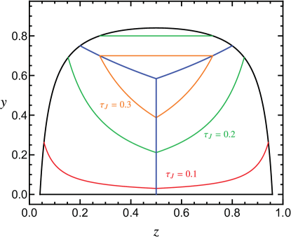
Figure 13: Three-particle phase space (black lines), thrust boundaries (blue lines) and constant $\tau_{J}$ value contour lines, with $\hat{m}=0.2$.

All integrals can be computed analytically, resulting in a long expression containing logs and dilogs. The expressions are available from the authors on request.

5.3 C-Jettiness

We finish the discussion on the computation of event-shape differential and cumulative distributions with the special case of $C_{J}$, whose contour lines are continuous and smooth, but can intersect with the phase-space boundaries in various ways, some of which are shown in Fig. 14. For the cumulative distribution one can find a simple expression that covers all possible scenarios

$$\Sigma^{1}_{C}(\bar{e}_{c})=R_{1}(\hat{m})-2\!\int_{z_{m}(e)}^{1/2}\!\mathrm{d}z\,\mathcal{M}_{C}[\,\min\{y_{\rm max}(z),y_{+}(e,z)\},y_{-}(e,z),z,\hat{m}]\,,$$ (73)

with $z_{m}$ the minimal value that $z$ can attain in the contour line within the phase-space boundaries. Therefore $z_{m}$ can be either $z_{\rm min}(e)$, the point at which the contour line has infinite slope, or $z_{-}^{\rm cut}$, the point at which it intersects with the phase-space boundary on the left side (if it intersects more than once, then the lower intersection has always smaller $z$ value). Analytic expressions for $y_{\pm}(z)$ can also be found. A careful examination of those and their interplay with $y_{\rm max}$ allows to find a general analytic expression for $z_{m}$. These results are given in Ref. Preisser:mthesis . The $z$ integration has to be performed numerically, and we use the quadpack package for that.

For the differential cross section one can also write down a unique expression by carefully defining the “upper” and lower contour lines

$$F_{e}(e,\hat{m})\,=\,2\!\int_{z_{m}(e)}^{1/2}\!\mathrm{d}z\sum_{y=y_{\pm}(e,z)}\Theta[y_{\rm max}(z)-y]\,\frac{M_{C}(y,z)}{y\,\Big{|}\frac{\mathrm{d}\hat{e}(y,z)}{\mathrm{d}y}\Big{|}}\,.$$ (74)

Here the Heaviside function splits the two $z$ integrals in various sub-integrals corresponding to different segments, which are sometimes disconnected. After a careful analysis one can disentangle all possible scenarios that Eq. (74) encompasses. These depend of course on the value of $C_{J}$, but also on $\hat{m}$. After working those out, the resulting $z$ integrals can be performed analytically in terms of incomplete Elliptic functions. A detailed computation, together with the final analytic expressions, is given in Ref. Preisser:mthesis .

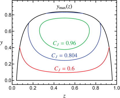
Figure 14: Three-particle phase space (black lines) showing contour lines for the C-jettiness event shape in red ($C_{J}=0.6$), blue ($C_{J}=0.804$) and green ($C_{J}=0.96$). The plot uses the numerical value $\hat{m}=0.3$.

6 Numerical Analysis

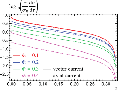
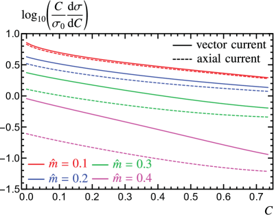
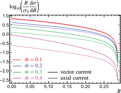
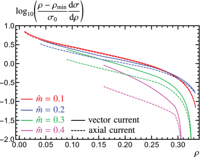
Figure 15: event-shape distributions for vector (solid curves) and axial-vector (dashed curves) currents. Panels (a), (b), (c), and (d) show results for thrust, C-parameter, jet broadening, and heavy jet mass, respectively. All curves are multiplied by $e-e_{\rm min}$, with $e$ the event-shape value and $e_{\rm min}$ its minimal value, such that the cross section is finite for $e=e_{\rm min}$. Red, blue, green and magenta lines show the results for $\hat{m}=0.1,\,0.2,\,0.3$ and $0.4$, respectively.

We start this section by showing differential cross section results for different values of $m/Q$ in Fig. 15. Since the only singular term at threshold diverges like $\sim 1/(e-e_{\rm min})$, we plot $(e-e_{\rm min})$ times the distribution, such that the curves are finite in the whole range. We also use a logarithmic scale on the $y$ axis to make the curves with small reduced mass value more visible. We show results for the most common event shapes, namely thrust, C-parameter, jet broadening and heavy jet mass in their original definition, although our code can yield results for those in any other scheme . With the exception of HJM, $e_{\rm min}$ and $e_{\rm max}$ are mass-independent, and therefore the main sensitivity of the cross section is through the magnitude of the curves: smaller masses result in larger cross sections in the tail. Vector and axial-vector cross sections are similar for small values of the reduced mass, but clearly different for e.g. $\hat{m}=0.4$. We observe that the axial-vector distributions are always lower than their vector counterparts. That hierarchy is also true for the plus and delta-function coefficients, as well as for the cumulative distribution. The HJM endpoints are mass-dependent, such that $\rho_{\min}$ [$\rho_{\max}$] increases [decreases] with $\hat{m}$. Therefore for this event shape (and all other mass-dependent ones) the mass sensitivity comes partly from the cross-section magnitude, but mainly from the peak position [the peak is not visible in the plots because of the $(\rho-\rho_{\rm min})$ factor, and the missing resummation and convolution with a non-perturbative shape function].

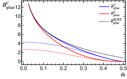
Figure 16: The universal coefficient of the plus distribution $B^{C}_{\rm plus}$ as a function of the reduced mass $\hat{m}$. We show the coefficient in the case of an axial-vector current (red solid line), a vector current (blue solid line) and the SCET limit (black dashed line). The SCET limit agrees with both the full QCD vector and axial cases in the limit $\hat{m}\to 0$. We also show the respective threshold limits as dotted lines, expanded up to $\mathcal{O}(v^{5})$. Both full QCD expressions approach zero in this limit, as expected.

In Fig. 16 we show the dependence of the plus-function coefficient on $\hat{m}$. For very small reduced masses one recovers the result predicted by SCET or bHQET,

$$B_{\text{plus}}^{\text{SCET}}=-2\,[\,1+2\log(\hat{m})\,]\,,$$ (75)

in which powers of $\hat{m}$ are suppressed and the mass-dependence is purely logarithmic. Since the squared matrix elements in QCD do not depend on $\log(\hat{m})$, the mass dependence of $B_{\text{plus}}^{\text{SCET}}$ must come from phase-space restrictions and the event shape definition. Hence, the massless limit has to be the same for both vector and axial-vector currents, as can be seen in Fig. 16 or by Taylor expanding the corresponding analytic formulas [ as in Eq. (75) ]. For $v\to 0$ both vector and axial-vector versions of $B_{\rm plus}$ tend to zero (faster for the axial current), which can be explained by physical arguments. In the threshold limit, all the energy coming from the $e^{+}e^{-}$ collision is invested in creating a heavy $q\bar{q}$ pair at rest. Therefore either no gluon (or massless quark) is radiated, or they have zero energy and momentum. No extra massive particles can be created. In this situation it is clear that $e=e_{\rm min}=e_{\rm max}$, and therefore there is no radiative tail. Hence both the plus distribution and non-singular cross section identically vanish, and only the delta function can remain. As a numerical check of the universality of $B^{C}_{\rm plus}$, shown in Fig. 16, we use the fact that

$$B_{\rm plus}=\lim_{e\to e_{\rm min}}(e-e_{\rm min})F_{e}(e,{\hat{m}})\,,$$ (76)

to determine graphically the plus-function coefficient for three distinct event shapes. For the vector and axial-vector currents separately, the cross sections approach the same horizontal line, matching our theoretical prediction. We have shown this behavior for $\hat{m}=0.1,\,0.2,\,0.3$ and $0.4$ in the four panels of Fig. 17. We have checked that universality holds for all $16$ event shapes considered in this article, and for $50$ values of the reduced mass. 

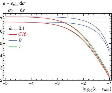
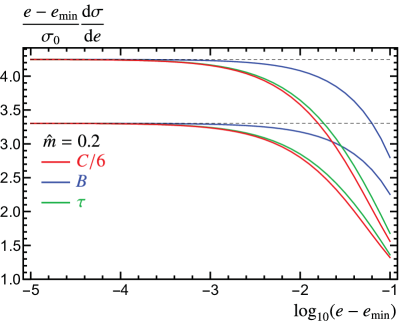
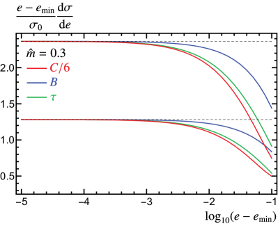
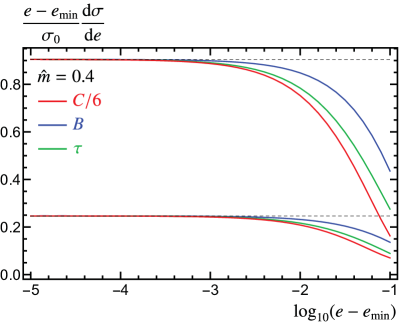
Figure 17: Numerical determination of the plus-function coefficient. Panels (a), (b), (c) and (d) correspond to $\hat{m}=0.1,\,0.2,\,0.3$ and $0.4$, respectively. In each panel curves converging to the upper (lower) horizontal dashed line show vector (axial-vector) current results. The dashed lines show the analytical result of $B_{\rm plus}$ for both currents. Thrust is shown in green, jet broadening in blue, and reduced C-parameter ($\widetilde{C}=C/6$) in red.

In Fig. 18 we show the $A_{e}^{C}$ coefficients as a function of the reduced mass for thrust, C-parameter, jet broadening and heavy jet mass. We again see that in the SCET/bHQET limit ($\hat{m}\to 0$), the result for both currents is the same. This follows from the same reasoning as in the previous paragraph. Moreover, since the axial total hadronic cross section vanishes for $v\to 0$, $A^{A}_{e}$ also vanishes in this limit. Furthermore, $A_{e}^{V}(\hat{m}=1/2)=R_{1}^{V}(v=0)=3\pi^{2}/4$ takes the same value for all event shapes in the limit $v\to 0$. This can be easily understood since the event-shape dependent integral in Eq. (40) appears multiplied in Eq. (3.3.3) precisely by the plus-function coefficient, and we already argued that in the threshold limit $B_{\rm plus}\to 0$. Another interesting property of the Dirac delta-function coefficient is that

$$\lim_{\hat{m}\to 0}[A_{e^{M}}(\hat{m})-A_{e^{P}}(\hat{m})]=\lim_{\hat{m}\to 0}[A_{e^{M}}(\hat{m})-A_{e^{E}}(\hat{m})]={\rm constant}\,,$$ (77)

where the constant is the difference of the Fourier-space jet functions in the massive and E/P schemes that appear in the bHQET factorization theorem for massive event shapes. This shall be shown in more detail in Ref. Alejandro-Vicent , but it is based on the fact that the hard and $H_{m}$ functions are the same for any event shape, and the soft function is the same in any scheme since it is mass independent at one loop order. Therefore the consistency condition requires that the jet anomalous dimensions and hence also the logs of $\hat{m}$ are the same in any scheme. Specifically, the logarithmic terms of the delta-function coefficients in the SCET limit $\hat{m}\to 0$ take the form

$$A_{e_{\mathrm{I}}}^{\text{SCET}}\Big{|}_{\log(\hat{m})}=4\log^{2}(\hat{m})+\log(\hat{m})\,,$$ (78)

for pure $\mathrm{SCET_{I}}$ type event shapes like thrust, heavy jet mass and C-parameter, and

$$A_{e_{\mathrm{II}}}^{\text{SCET}}\Big{|}_{\log(\hat{m})}=2\log^{2}(\hat{m})-\log(\hat{m})\,,$$ (79)

for $\mathrm{SCET_{II}}$ type ones like jet broadening. For similar reasons, the SCET/bHQET limit is equal for the same event shape in the E or P scheme, as well as with normalization $Q$ or $Q_{P}$.

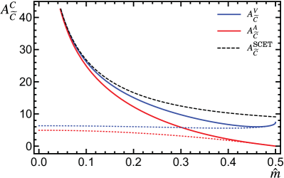
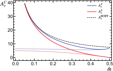
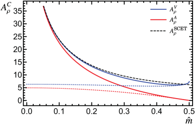
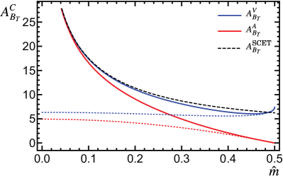
Figure 18: The delta-function coefficients for reduced C-parameter, thrust, heavy jet mass and jet broadening (all in their original definitions) as a function of the reduced mass $\hat{m}$. The red solid lines show the coefficients for an axial-vector current, the blue solid lines for a vector current. We also show the respective threshold limits as dotted lines, including terms up to $\mathcal{O}(v^{2})$. The SCET limit, shown as black dashed lines, coincides with the vector as well as axial currents for $\hat{m}\to 0$. The values in the threshold limit are universal, approaching $3\pi^{2}/4$ and zero in the vector and axial-vector cases, respectively.

In Fig. 19 we use Eq. (59) to graphically determine the delta-function coefficient, checking that it agrees with our analytic computation. To make it visually clearer, we use logarithmic scaling in the horizontal axis, such that the log-subtracted cumulative distribution becomes a horizontal line as the event-shape value approaches the threshold. This plot also shows how reliable our numerical code is, even for very small values of the event shape. We choose the same event-shape measurement functions and reduced-mass values as for the rest of analyses in this section.

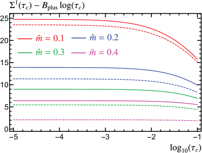
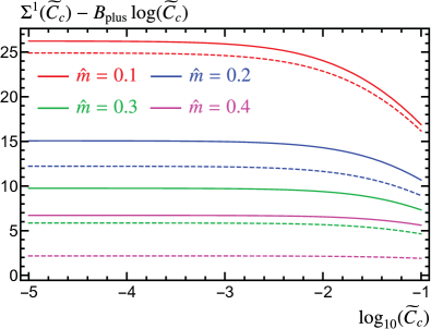
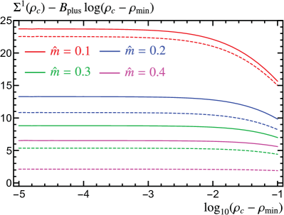
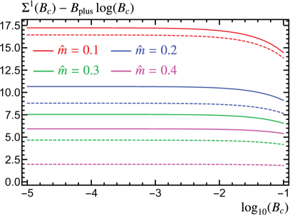
Figure 19: Numerical determination of the delta-function coefficient. Panel (a) is for thrust, (b) for reduced C-parameter, (c) for heavy jet mass and (d) for jet broadening, respectively. Solid (dashed) lines show the vector (axial-vector) current. Red, blue, green and magenta have reduced masses of $\hat{m}=0.1,\,0.2\,0.3$ and $0.4$, respectively. Each curve becomes a horizontal line as the event shape approaches its minimal value, reproducing exactly our analytic computations for $A_{e}$.

7 Conclusions

In this article we have shown how to accurately compute differential and cumulative massive event-shape distributions at $\mathcal{O}(\alpha_{s})$. We have analytically calculated all singular terms: the plus-distribution coefficient, which we found to be the same for all event shapes linearly sensitive to soft momenta, and the delta-function coefficient. In our computation of the latter we add the contributions of virtual- and real-radiation diagrams, which are individually IR-divergent, although the sum is finite. We find that the delta-function coefficient only depends on the soft limit of the event-shape measurement function, and can be expressed as the sum of a universal term plus an observable-dependent integral times the plus-function coefficient.

We have developed a numerical algorithm to compute the non-singular distribution efficiently and with high accuracy which does not require binning the distributions. The method directly solves the measurement delta function and figures out the integration limits using standard numerical methods to find the roots of an equation or to minimize functions. The remaining integration is performed numerically. Our method serves for both differential and cumulative cross sections, can be used for massless quarks, and provides very accurate results even for extreme dijet configurations. Possible additional applications of the algorithm are a) event-shape distributions depending on a continuous parameter, such as angularities; b) non-global observables implying a jet algorithm and grooming, such as Soft Drop Larkoski:2014wba . Our approach is very different from conventional MC methods, which are based on binned distributions. Although at $\mathcal{O}(\alpha_{s})$ one does not yet need to implement subtractions, our strategy to compute the delta-function coefficient could be implemented in NLO parton-level MCs to achieve a much more effective cancellation of IR divergences, that could happen at an early stage.

Extending our calculation of the singular terms to $\mathcal{O}(\alpha_{s}^{2})$ could be possible, provided one can find an analytic form for the event-shape measurement function in the soft limit. Computing the next order could provide hints to figure out if the universality of the plus distribution holds to all orders. Another approach to compute the delta and plus distributions at two loops is using EFT language. Since these parameters are defined in the limit of very soft gluon momenta, one can imagine building an EFT of heavy quarks (not necessarily boosted) interacting with soft particles (massless quarks or gluons), such that $E_{\rm soft}\ll m_{q}$. In this way one could derive a factorized form for the cross section in terms of a universal matching coefficient and an event-shape dependent soft function. This could simplify the computation, since the cross section provided by the EFT would be already purely singular, and the problem would be naturally split into simpler pieces, treating one scale at a time. Moreover, such a theory would allow to sum large logarithms of ratios of scales to all orders in perturbation theory. A step in this direction has been taken already in Ref. vonManteuffel:2014mva .

Our results will be a reference for ongoing and future research carried out in the context of event shapes with massive particles. In particular they will play an important role in the calibration of the MC top quark mass parameter, and will be even more relevant for the top quark mass measurement program at future linear colliders. In this direction, the results presented in this article will help computing efficiently $e^{+}e^{-}$ event-shape distributions at $\mathcal{O}(\alpha_{s})$ for unstable top quarks, since in that case, the delta function that sits at threshold for stable quarks radiates into the tail through the top decay products. Therefore, already at $\mathcal{O}(\alpha_{s})$ one has to deal with the cancellation of IR divergences away from threshold, and our strategy for computing the delta-function coefficient could be adapted for this situation.

Appendix A Indirect Computation

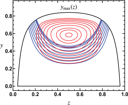
Figure 20: Phase space diagram in $(z,y)$ coordinates (black lines) showing curves with constant value of the C-parameter event-shape measurement function (in red) and for its soft limit (in blue), for the same set of $C$ values $\{0.42,0.468,0.516,0.564,0.612,0.66,0.708,0.729,0.747\}$, while $\hat{m}=0.2$. Red curves are always contained withing the phase-space boundaries, and the enclosed area becomes smaller as the value of $C$ approaches its maximum value, when it collapses to a single point. Blue curves always intersect with the phase-space boundary, and have a finite extension even for $C=C_{\rm max}$. Blue and red curves are similar for small values of $y$.

In this appendix we recover the main result of Eq. (3.3.3) imposing that the integrated event-shape distribution over its entire domain reproduces the known total hadronic cross section. This method was discussed in the introduction as a way of obtaining, in a numeric form, the delta-function coefficient if an analytic form for the differential cross section is available in $d=4$ dimensions. Here we show that if the event shape integration is performed before the phase-space integrals, analytic results can be obtained for any event shape considered in this article. Moreover, the result is equivalent to what we have already found by the direct computation.

Writing the massive total hadronic cross section as

$$R(\hat{m})=R_{0}(\hat{m})+C_{F}\frac{\alpha_{s}}{\pi}R_{1}(\hat{m})+\mathcal{O}(\alpha^{2}_{s})\,,$$ (80)

one observes the non-trivial constraint

$$R_{1}(\hat{m})=A_{e}(\hat{m})+B_{\rm plus}(\hat{m})\log(e_{\max}-e_{\min})+\int^{e_{\max}}_{e_{\min}}\mathrm{d}e\,F^{\rm NS}(e,\hat{m})\,,$$ (81)

where $F^{\rm NS}_{e}$, defined in Eq. (37), has to be integrated in the whole $e$ domain $[e_{\min},e_{\max}]$. This is done before integrating in $y$ and $z$. The $e$ integration in $F^{\rm NS}_{\rm hard}$ effectively only replaces the Dirac delta function by $1$, since the entire phase space is exactly covered by the full event shape range,

$$\int^{e_{\max}}_{e_{\min}}\!\mathrm{d}e\,F^{\rm NS}_{\rm hard}(e,\hat{m})=\!\int\!\mathrm{d}z\,\mathrm{d}y\,M^{\rm hard}_{C}(y,z,\hat{m})\,.$$ (82)

It is convenient to write the soft non-singular distribution with explicit Heaviside functions in $y$, such that the two terms with the soft measurement function in Eq. (37) can be added together

$$F^{\rm NS}_{\rm soft}=\int\!\mathrm{d}z\,\mathrm{d}y\,\frac{M_{C}^{0}(z,\hat{m})}{y}\,\Theta(y)\biggl{\{}\Theta[y_{\max}(z)-y]\,\delta[e-\hat{e}(y,z)]-\delta[e-\bar{e}(y,z)]\biggl{\}}\,,$$ (83)

understanding that the $z$ integration is still between $z_{-}$ and $z_{+}$. To evaluate the $F^{\rm NS}_{\rm soft}$ contribution it is convenient to insert $\Theta(e_{\max}-e)$ before performing the $e$ integral over the Dirac delta functions. In this way we obtain

$$\int^{e_{\max}}_{e_{\min}}\mathrm{d}e\,F^{\rm NS}_{\rm soft}(e,\hat{m})=\int\!\mathrm{d}z\,\mathrm{d}y\,\frac{M^{0}_{C}(z,\hat{m})}{y}\,\Theta(y)\Bigl{\{}\Theta[y_{\max}(z)-y]-\Theta[h(e_{\rm max},z)-y]\Bigl{\}}\,.$$ (84)

Graphically, the integral of the first term corresponds to the areas marked as II, III and IV in Fig. 21, while the second integral is the sum of regions I, III and IV. The sum of III and IV corresponds to integrating the last term in Eq. (37), while the pieces marked with I are the integration of the one-to-last term in Eq. (37).

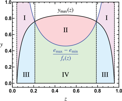
Figure 21: Phase space diagram in $(z,y)$ coordinates (black lines) showing the curve for which the C-parameter soft measurement function equals the maximum allowed value $C_{\rm max}=0.75$. Different colors correspond to the different integration regions of the soft non-singular distribution. To make this plot we use the numerical value $\hat{m}=0.2$.

Adding the two terms, the resulting $y$ integration has the boundaries $[h(e_{\max},z),y_{\max}(z)]$ in the whole $z$ range, which can be expressed as

$$\int^{e_{\max}}_{e_{\min}}\mathrm{d}e\,F^{\rm NS}_{\rm soft}(e,\hat{m})=\int_{z_{-}}^{z_{+}}\!\mathrm{d}z\,M^{0}_{C}(z,\hat{m})\log\Biggl{[}\frac{1-\frac{\hat{m}^{2}}{z(1-z)}}{\frac{e_{\max}-e_{\min}}{f_{e}(z,\hat{m})}}\Biggr{]}\,,$$ (85)

and graphically corresponds to subtracting the portions marked with I from the area labeled II in Fig. 21. Combining this result with the plus function term and using Eq. (37) the dependence on $e_{\rm max}$ cancels. The $y$ integration can be performed analytically, giving

$$B_{\rm plus}(\hat{m})\log(e_{\max}-e_{\min})+\!\int^{e_{\max}}_{e_{\min}}\!\mathrm{d}e\,F^{\rm NS}_{\rm soft}(e,\hat{m})$$

$$=\int\!\mathrm{d}z\,M^{0}_{C}(z,\hat{m})\biggl{\{}\log\biggl{[}1-\frac{\hat{m}^{2}}{z(1-z)}\biggr{]}+\log[f_{e}(z)]\biggl{\}}\,,$$ (86)

$$\!\!\!\int\!\mathrm{d}y\,\mathrm{d}z\,M^{{\rm hard}}_{C}(y,z)=\!\int\!\mathrm{d}z\,\biggl{(}1-\frac{\hat{m}^{2}}{z(1-z)}\biggr{)}\biggl{[}M^{2}_{C}(z,\hat{m})+\frac{1}{2}M^{3}_{C}(z,\hat{m})\biggl{(}1-\frac{\hat{m}^{2}}{z(1-z)}\biggr{)}\biggr{]}.$$

With this we conclude with the alternative, but analytically equivalent, expression for the $\delta$ coefficient

$$A_{e}(\hat{m})={} R_{1}(\hat{m})-\!\int_{z_{-}}^{z_{+}}\!\mathrm{d}z\,\biggl{\{}M^{0}_{C}(z,\hat{m})\bigl{[}\log\bigl{[}z(1-z)-m^{2}\bigr{]}-\log[z(1-z)]+\log[f_{e}(z)]\,\bigr{]}$$

$$+\biggl{(}1-\frac{\hat{m}^{2}}{z(1-z)}\biggr{)}\biggl{[}M^{2}_{C}(z,\hat{m})+\frac{1}{2}M^{3}_{C}(z,\hat{m})\biggl{(}1-\frac{\hat{m}^{2}}{z(1-z)}\biggr{)}\biggr{]}\biggl{\}}.$$ (87)

The integral over hard matrix elements can be performed using Eqs. (90), while the other integrals are explicitly given in Eqs. (B). Using these analytic results we arrive at

$$A^{V}_{e}(\hat{m}) = R^{V}_{1}(\hat{m})-(3-v^{2})I_{e}(\hat{m})-(1+2\hat{m}^{4})L_{v}-\frac{v}{4}\biggl{[}11+34\hat{m}^{2}-8(3-v^{2})\log\Bigl{(}\frac{v}{\hat{m}}\Bigr{)}\biggr{]}$$

$$\!\!\!\!\!+2\,v^{2}\biggl{[}{\rm Li}_{2}\biggl{(}\frac{2v}{1+v}\biggr{)}-2\log\Bigl{(}\frac{v^{2}}{\hat{m}}\Bigr{)}L_{v}+\,{\rm Li}_{2}\biggl{(}\frac{1-v}{2}\biggr{)}-{\rm Li}_{2}\biggl{(}\frac{2v}{v-1}\biggr{)}-{\rm Li}_{2}\biggl{(}\frac{1+v}{2}\biggr{)}\biggr{]},$$

$$A^{A}_{e}(\hat{m}) = R^{A}_{1}(\hat{m})-2v^{2}I_{e}(\hat{m})-(1+2\hat{m}^{2}-6\hat{m}^{4}+12\hat{m}^{6})L_{v}-\frac{v}{4}\biggl{[}11-68\hat{m}^{2}+12\hat{m}^{4}$$ (88)

$$\!\!\!\!\!-16v^{2}\log\Bigl{(}\frac{v}{\hat{m}}\Bigr{)}\biggr{]}+2(1-6\hat{m}^{2}+8\hat{m}^{4})\biggl{[}{\rm Li}_{2}\biggl{(}\frac{2v}{1+v}\biggr{)}+{\rm Li}_{2}\biggl{(}\frac{1-v}{2}\biggr{)}$$

$$\!\!\!\!\!-\,2\log\Bigl{(}\frac{v^{2}}{\hat{m}}\Bigr{)}L_{v}-{\rm Li}_{2}\biggl{(}\frac{2v}{v-1}\biggr{)}-{\rm Li}_{2}\biggl{(}\frac{1+v}{2}\biggr{)}\biggr{]}.$$

Using the known results for the total hadronic cross section, collected for convenience in Eq. (C) of Appendix C, it can be checked that the above result is analytically equivalent to Eqs. (3.3.3).

Appendix B Phase-Space Integrals

Almost every integral in the phase-space variable $z$ we have computed for various event-shape measurement functions can, due to the symmetry under $z\to 1-z$, be cast in the one these forms:

$$\int^{z_{+}}_{\frac{1}{2}}\mathrm{d}z\frac{\log(z-a)}{z}={} {\rm Li}_{2}\biggl{(}1-\frac{1+v}{2a}\biggr{)}+\log\Bigl{(}\frac{1+v}{2a}\Bigr{)}\log\biggl{(}\frac{1-2a+v}{2}\biggr{)}$$ (89)

$$-{\rm Li}_{2}\biggl{(}1-\frac{1}{2a}\biggr{)}+\log\biggl{(}\frac{1}{2}-a\biggr{)}\log(2a)\,,\quad a\leq\frac{1}{2}\,,$$

$$\int^{z_{+}}_{\frac{1}{2}}\mathrm{d}z\frac{\log(a-z)}{z}={} {\rm Li}_{2}\biggl{(}1-\frac{1+v}{2a}\biggr{)}+\log\Bigl{(}\frac{1+v}{2a}\Bigr{)}\log\Bigl{(}\frac{2a-1-v}{2}\Bigr{)}$$

$$-{\rm Li}_{2}\biggl{(}1-\frac{1}{2a}\biggr{)}+\log\Bigl{(}a-\frac{1}{2}\Bigr{)}\log(2a)\,,\quad a\geq z_{+}\,,$$

$$\int^{z_{+}}_{\frac{1}{2}}\mathrm{d}z\frac{\log(z-a)}{z^{2}}={} \frac{1}{a}\Biggl{\{}\log\Bigl{(}\frac{1-2a+v}{1+v}\Bigr{)}-2a\log(2)-(1-2a)\log(1-2a)$$

$$-\,\frac{2a\log\Bigl{(}\frac{1-2a+v}{2}\Bigr{)}}{1+v}\Biggl{\}},\quad a\leq\frac{1}{2}\,,$$

$$\int^{z_{+}}_{\frac{1}{2}}\mathrm{d}z\frac{\log(a-z)}{z^{2}}={} \frac{1}{a}\Biggl{\{}\log\Bigl{(}-\frac{1-2a+v}{1+v}\Bigr{)}-2\,a\log(2)-(1-2a)\log(2a-1)$$

$$-\,\frac{2a\log\Bigl{(}-\frac{1-2a+v}{2}\Bigr{)}}{1+v}\Biggl{\}},\quad a\geq z_{+}\,.$$

For integrals in which no event-shape measurement function is involved, the results are even simpler

$$\int^{z_{+}}_{z_{{}_{-}}}\!\!\mathrm{d}z =v\,,\qquad\qquad\qquad\int^{z_{+}}_{z_{{}_{-}}}\!\!\frac{\mathrm{d}z}{z}=\!\int^{z_{+}}_{z_{{}_{-}}}\!\frac{\mathrm{d}z}{1-z}=2\,L_{v}\,,$$ (90)

$$\int^{z_{+}}_{z_{{}_{-}}}\!\frac{\mathrm{d}z}{z^{2}} =\int^{z_{+}}_{z_{{}_{-}}}\!\frac{\mathrm{d}z}{(1-z)^{2}}=\frac{v}{\hat{m}^{2}},\qquad\int^{z_{+}}_{z_{{}_{-}}}\!\frac{\mathrm{d}z}{z^{3}}=\int^{z_{+}}_{z_{{}_{-}}}\!\frac{\mathrm{d}z}{(1-z)^{3}}=\frac{v}{2\hat{m}^{4}}\,,$$

$$\int^{z_{+}}_{z_{{}_{-}}}\!\!\mathrm{d}z\frac{\log[z(1-z)-\hat{m}^{2}]}{z^{2}} =\!\int^{z_{+}}_{z_{{}_{-}}}\!\!\mathrm{d}z\frac{\log[z(1-z)-\hat{m}^{2}]}{(1-z)^{2}}=\frac{2v\log(v)-2L_{v}}{\hat{m}^{2}}\,,$$

$$\int^{z_{+}}_{z_{{}_{-}}}\!\!\mathrm{d}z\frac{\log[z(1-z)-\hat{m}^{2}]}{z} =\!\int^{z_{+}}_{z_{{}_{-}}}\!\!\mathrm{d}z\frac{\log[z(1-z)-\hat{m}^{2}]}{1-z}={\rm Li}_{2}\Bigl{(}\frac{2v}{v-1}\Bigr{)}-{\rm Li}_{2}\Bigl{(}\frac{2v}{1+v}\Bigr{)}+4\log(v)L_{v}\,.$$

With these one can easily compute the integrals for the real radiation contribution

$$\qquad\qquad\qquad\qquad\int^{z_{+}}_{z_{{}_{-}}}\!\!\mathrm{d}z\,\frac{(1-z)z-\hat{m}^{2}}{(1-z)^{2}z^{2}}=\,2\bigl{[}(1+v^{2})L_{v}-v\bigr{]}$$

$$\int^{z_{+}}_{z_{{}_{-}}}\!\!\mathrm{d}z\,\frac{(1-z)z-\hat{m}^{2}}{(1-z)^{2}z^{2}}\log[z(1-z)-\hat{m}^{2}]=\,4\,L_{v}-4\,v\log(v)+(1+v^{2})\biggl{[}{\rm Li}_{2}\Bigl{(}\frac{2v}{v-1}\Bigr{)}$$

$$\qquad\qquad\qquad\qquad\qquad-{\rm Li}_{2}\Bigl{(}\frac{2v}{1+v}\Bigr{)}+4\log(v)\,L_{v}\biggr{]}\,,$$ (91)

$$\int^{z_{+}}_{z_{{}_{-}}}\!\!\mathrm{d}z\,\frac{(1-z)z-\hat{m}^{2}}{(1-z)^{2}z^{2}}\log[z(1-z)]=\,(1+v^{2})\biggl{[}{\rm Li}_{2}\Bigl{(}\frac{1-v}{2}\Bigr{)}-{\rm Li}_{2}\Bigl{(}\frac{1+v}{2}\Bigr{)}\biggr{]}$$

$$\qquad\qquad\qquad\qquad\qquad+2\bigl{[}(1+v^{2})\log(\hat{m})+4\hat{m}^{2}\bigr{]}L_{v}-2v\bigl{[}1+2\log(\hat{m})\bigr{]}\,.$$

Note that the integrands given in Eq. (B) are invariant under the substitution $z\to(1-z)$ and therefore $\int^{z_{+}}_{z_{{}_{-}}}\mathrm{d}z=2\int^{1/2}_{z_{-}}\mathrm{d}z=2\int^{z_{+}}_{1/2}\mathrm{d}z$.

Appendix C Total Hadronic Cross Section

It is convenient to write the total hadronic cross section in the following way, such that it can be implemented in Eq. (A)

$$R^{V}_{1}(\hat{m}) = 4(1-4\hat{m}^{4})\biggl{[}3L_{v}^{2}+2\,{\rm Li}_{2}\biggl{(}\frac{1-v}{v+1}\biggr{)}+{\rm Li}_{2}\biggl{(}\frac{v-1}{v+1}\biggr{)}-\log\Bigl{(}\frac{v^{2}}{\hat{m}^{3}}\Bigr{)}L_{v}\biggr{]}$$

$$+\,2(3-2\hat{m}^{2}-7\hat{m}^{4})L_{v}+v\biggl{[}\frac{3}{4}(1+6\hat{m}^{2})-(3-v^{2})\log\Bigl{(}\frac{v^{2}}{\hat{m}^{3}}\Bigr{)}\biggr{]},$$

$$R^{A}_{1}(\hat{m}) = 2\,v^{2}(1+v^{2})\biggl{[}3\,L_{v}^{2}+2\,{\rm Li}_{2}\biggl{(}\frac{1-v}{v+1}\biggr{)}+{\rm Li}_{2}\biggl{(}\frac{v-1}{v+1}\biggr{)}-\log\Bigl{(}\frac{v^{2}}{\hat{m}^{3}}\Bigr{)}L_{v}\biggr{]}$$

$$+\,2(3-11\hat{m}^{2}+5\hat{m}^{4}+6\hat{m}^{6})L_{v}-\frac{21}{16}v-v^{3}\biggl{[}2\log\Bigl{(}\frac{v^{2}}{\hat{m}^{3}}\Bigr{)}-\frac{15}{8}-\frac{3}{16}v^{2}\biggr{]},$$

coinciding with Ref. Chetyrkin:1994js .

Appendix D Analytic Delta-Function Coefficients for some Event Shapes

In this appendix we present some analytic results for the delta-function coefficient of massive event-shape differential cross sections. Specifically, we list the following information:

• The general definition of the event shape $e$.

• The expression $e_{q}(y,z)$ describing the event shape in the phase-space region in which the thrust axis $\hat{t}$ is aligned with the quark momentum in terms of $y,z$. When evaluating the integral $I_{e}$, we use the $z\leftrightarrow(1-z)$ symmetry and integrate only in this region.

• The minimal value of the event shape $e_{\text{min}}$, valid to all orders in perturbation theory.

• The maximal value of the event shape $e_{\text{max}}$, valid at one-loop level.

• The soft term $f_{e}(z)$ of the event shape required for the integral $I_{e}$, derived from $e_{q}(y,z)$ and therefore valid in the same phase-space region only. It is straight forward to obtain the expression for the region where $\hat{t}$ is proportional to the anti-quark momentum by applying the substitution $z\to(1-z)$.

• The solution of the integrals $I_{e}(\hat{m})$, which can be inserted into Eq. (3.3.3) or (A) to obtain the delta-function coefficient $A_{e}^{C}$.

For simplicity, we define

$$r={} \sqrt{1-3\hat{m}^{2}}\,,\qquad\text{mod}(y,z)=\sqrt{(1-yz)^{2}-4\hat{m}^{2}}\,,$$

$$\mathcal{I}(\hat{m})\equiv{} \int_{z_{-}}^{\frac{1}{2}}\mathrm{d}z\,\frac{z(1-z)-\hat{m}^{2}}{z^{2}(1-z)^{2}}=\bigl{(}1+v^{2}\Bigr{)}L_{v}-v\,,$$ (93)

frequently appearing in expressions for $e_{\text{max}}$, $e_{q}(y,z)$ and relations between event shapes, respectively. Moreover, we use the pseudo-rapidity $\eta$, transverse momentum $p_{\bot}\equiv|\vec{p}_{\bot}|$ and transverse mass $m_{\bot}\equiv\sqrt{p_{\bot}^{2}+m^{2}}$ in some event-shape definitions, where the transverse momentum is measured with respect to the thrust axis. The solutions of the integrals needed to compute the various expressions for $I_{e}(\hat{m})$, are provided in Appendix B.

Sometimes it can be useful to define a P-scheme event shape $e^{P,Q}$ with $1/Q^{n}$ normalization instead of $1/Q_{P}^{n}$. The relation between the related event shape dependent integrals $I_{e}(\hat{m})$ is trivial, as long as $e_{\text{min}}=0$:

$$I_{e^{P,Q}}(\hat{m})=I_{e^{P}}(\hat{m})+n\log(v)\,\mathcal{I}(\hat{m})\,.$$ (94)

Heavy Jet Mass

Original definition

• $\rho=\frac{1}{Q^{2}}\Bigl{(}\sum_{i\in\text{heavy}}p_{i}\Bigr{)}^{\!2}$

• $\rho_{q}(y,z)=\hat{m}^{2}+yz$

• $\rho_{\text{min}}=\hat{m}^{2}$

• $\rho_{\text{max}}=(5-4r)/3$

• $f_{\rho}(z)=z$

• $\begin{aligned} I_{\rho}(\hat{m})\,={}&\frac{1}{4}\biggl{[}(1+v^{2})\text{Li}_{2}\biggl{(}\frac{v+1}{v-1}\biggr{)}+\frac{\pi^{2}}{6}(1+v^{2})-2v(v+1)\\ &-[1+(4-v)v]\log\biggl{(}\frac{1-v}{1+v}\biggr{)}-4v\log\biggl{(}\frac{v+1}{2}\biggr{)}\biggr{]}\end{aligned}$

P-scheme

• $\rho^{P}=\frac{1}{Q_{P}^{2}}\sum_{i,j\in\text{heavy}}(|\vec{p}_{i}||\vec{p}_{j}|-\vec{p}_{i}\cdot\vec{p}_{j})$

• $\rho^{P}_{q}(y,z)=\frac{Q^{2}}{2Q_{P}^{2}}y\bigl{[}\text{mod}(y,1-z)+y(1-z)+2z-1\bigr{]}$

• $\rho^{P}_{\text{min}}=0$

• $\rho^{P}_{\text{max}}=1/3$

• $f_{\rho^{P}}(z)=\frac{2z+v-1}{2v^{2}}$

• $\begin{aligned} I_{\rho^{P}}(\hat{m})={}&(1-2\hat{m}^{2})\biggl{[}\text{Li}_{2}(1-v)+\text{Li}_{2}\biggl{(}\frac{1}{v+1}\biggr{)}\biggr{]}\\ &+\frac{1}{2}\log\biggl{(}\frac{1+v}{1-v}\biggr{)}[1-2(1-2\hat{m}^{2})\log(2v^{2})]-\frac{1}{2}(1-2\hat{m}^{2})\log^{2}(1-v)\\ &-\frac{1}{3}(1-2\hat{m}^{2})[\pi^{2}-3\log^{2}(v+1)]-v\log(\hat{m})+v\log(v)\end{aligned}$

E-scheme

• $\rho^{E}=\frac{1}{Q^{2}}\sum_{i,j\in\text{heavy}}\frac{E_{i}E_{j}}{|\vec{p}_{i}||\vec{p}_{j}|}(|\vec{p}_{i}||\vec{p}_{j}|-\vec{p}_{i}\cdot\vec{p}_{j})$

• $\rho^{E}_{q}(y,z)=\frac{y(1-y(1-z))[\text{mod}(y,1-z)+y(1-z)-1+2z]}{2\,\text{mod}(y,1-z)}$

• $\rho^{E}_{\text{min}}=0$

• $\rho^{E}_{\text{max}}=\frac{(2-r)^{2}}{3}$

• $f_{\rho^{E}}(z)=vf_{\rho^{P}}(z)$

• $I_{\rho^{E}}(\hat{m})=I_{\rho^{P}}(\hat{m})+\log(v)\,\mathcal{I}(\hat{m})$

Thrust / 2-Jettiness

P-scheme, original definition

• $\tau=\frac{1}{Q_{P}}\sum_{i}p_{i,\bot}\mathrm{e}^{-|\eta_{i}|}=\frac{1}{Q_{P}}\min_{\hat{t}}\sum_{i}(|\vec{p}_{i}|-|\hat{t}\cdot\vec{p}_{i}|)$

• $\tau_{q}(y,z)=\text{mod}(y,1-z)-\text{mod}(y,z)+y$

• $\tau_{\text{min}}=0$

• $\tau_{\text{max}}=\rho^{P}_{\text{max}}$

• $f_{\tau}(z)=f_{\rho^{P}}(z)$

• $I_{\tau}(\hat{m})=I_{\rho^{P}}(\hat{m})$

E-scheme

• $\tau^{E}=\frac{1}{Q_{P}}\min_{\hat{t}}\sum_{i}\frac{E_{i}}{|\vec{p}_{i}|}(|\vec{p}_{i}|-|\hat{t}\cdot\vec{p}_{i}|)$

• $\tau^{E}_{q}(y,z)=\frac{1}{2}\biggl{(}\frac{[1-y(1-z)][4\hat{m}^{2}+y^{2}(1-z)z-1+y]}{\text{mod}(y,z)\,\text{mod}(y,1-z)}-\frac{y[1+(y-2)z]}{\text{mod}(y,z)}-y(1-z)+1+y\biggr{)}$

• $\tau^{E}_{\text{min}}=0$

• $\tau^{E}_{\text{max}}=\rho^{E}_{\text{max}}$

• $f_{\tau^{E}}(z)=f_{\rho^{E}}(z)$

• $I_{\tau^{E}}(\hat{m})=I_{\rho^{E}}(\hat{m})$

2-jettiness

• $\tau_{J}=\frac{1}{Q}\sum_{i}m_{i,\bot}\mathrm{e}^{-|\eta_{i}|}=\frac{1}{Q}\min_{\hat{t}}\sum_{i}(E_{i}-|\hat{t}\cdot\vec{p}_{i}|)$

• $\tau_{J,q}(y,z)=1-\text{mod}(y,z)$

• $\tau_{J,\,\text{min}}=1-v$

• $\tau_{J,\,\text{max}}=\rho_{\text{max}}$

• $f_{\tau_{J}}(z)=z/v$

• $I_{\tau_{J}}(\hat{m})=I_{\rho}(\hat{m})-\log(v)\,\mathcal{I}(\hat{m})$

C-Parameter / C-Jettiness

Here we provide results for reduced C-parameter $\widetilde{C}=C/6$. The relation to the original version for the event shape dependent integral is simply

$$I_{C}(\hat{m})=I_{\widetilde{C}}(\hat{m})-\log(6)\,\mathcal{I}(\hat{m})\,.$$ (95)

P-scheme, original definition

• $\widetilde{C}=\frac{1}{4}\Bigl{[}1-\frac{1}{Q_{P}^{2}}\sum_{i,j}\frac{(\vec{p}_{i}\cdot\vec{p}_{j})^{2}}{|\vec{p}_{i}||\vec{p}_{j}|}\Bigr{]}$

• $\widetilde{C}_{q}(y,z)=\frac{2y\,[(1-y)(1-z)z-\hat{m}^{2}]}{\text{mod}(y,1-z)\,\text{mod}(y,z)[\text{mod}(y,1-z)+\text{mod}(y,z)+y]}$

• $\widetilde{C}_{\text{min}}=0$

• $\widetilde{C}_{\text{max}}=1/8$

• $f_{\widetilde{C}}(z)=\frac{(1-z)z-\hat{m}^{2}}{v^{3}}$

• $\begin{aligned} I_{\widetilde{C}}(\hat{m})\,={}&(1-2\hat{m}^{2})\biggl{[}-2\log^{2}(2\hat{m})+2\,\text{Li}_{2}\biggl{(}\frac{1-v}{1+v}\biggr{)}+2\log^{2}(1+v)-\frac{\pi^{2}}{3}\\ &+3\log(v)\log\biggl{(}\frac{1-v}{1+v}\biggr{)}+2\log(2)\log\biggl{(}\frac{1-v}{1+v}\biggr{)}\biggr{]}+v\log(v)-\log\biggl{(}\frac{1-v}{1+v}\biggr{)}\end{aligned}$

E-scheme

• $\widetilde{C}^{E}=\frac{1}{4}\Bigl{[}1-\frac{1}{Q^{2}}\sum_{i,j}\frac{E_{i}E_{j}(\vec{p}_{i}\cdot\vec{p}_{j})^{2}}{|\vec{p}_{i}|^{2}|\vec{p}_{j}|^{2}}\Bigr{]}$

• $\widetilde{C}^{E}_{q}(y,z)\!=\!\frac{y\{\hat{m}^{2}[y(6(1-z)z+1)-3y^{2}(1-z)z-4(1-z)z-1]-2\hat{m}^{4}(y-2)+(1-y)(1-z)z[1-y(1-z)](1-yz)\}}{\text{mod}^{2}(y,z)\,\,\text{mod}^{2}(y,1-z)}$

• $\widetilde{C}^{E}_{\text{min}}=0$

• $\widetilde{C}^{E}_{\text{max}}=1/8$

• $f_{\widetilde{C}^{E}}(z)=vf_{\widetilde{C}}(z)$

• $I_{\widetilde{C}^{E}}(\hat{m})=I_{\widetilde{C}}(\hat{m})+\log(v)\,\mathcal{I}(\hat{m})$

C-jettiness

• $\widetilde{C}_{J}=\frac{1}{4}\Bigl{[}2-\frac{1}{Q^{2}}\sum_{i\neq j}\frac{(p_{i}\cdot p_{j})^{2}}{E_{i}E_{j}}\Bigr{]}$

• $\widetilde{C}_{J,q}(y,z)=\frac{z(1-z)y(1-y)+2\hat{m}^{2}(1-y)-2\hat{m}^{4}}{(1-zy)[1-(1-z)y]}$

• $\widetilde{C}_{J,\,\text{min}}=2\hat{m}^{2}(1-\hat{m}^{2})$

• $\widetilde{C}_{J,\,\text{max}}=\begin{cases}(1+16\hat{m}^{2}+32\hat{m}^{4})/(1+2\hat{m}^{2})^{2}/8\quad&(\hat{m}<0.39307568887871164)\\ 4\hat{m}^{2}(1+2\hat{m}^{2})/(1+4\hat{m}^{2})^{2}\quad&(\hat{m}>0.39307568887871164)\end{cases}$

• $f_{\widetilde{C}_{J}}(z)=z(1-z)-2\hat{m}^{4}$

• $\begin{aligned} I_{\widetilde{C}_{J}}(\hat{m})={}&\frac{1}{2}(2\hat{m}^{2}-1)\biggl{\{}-2\text{Li}_{2}\biggl{(}\frac{1-v}{1+u}\biggr{)}+2\,\text{Li}_{2}\biggl{(}\frac{1-u}{1-v}\biggr{)}-2\,\text{Li}_{2}\biggl{(}\frac{1-u}{1+v}\biggr{)}\\ &+2\,\text{Li}_{2}\biggl{(}\frac{1+v}{1+u}\biggr{)}+\log^{2}\biggl{(}\frac{1-v}{1+v}\biggr{)}+2\log\biggl{(}\frac{1-v}{1+v}\biggr{)}\log\biggl{[}\frac{(1+u)(1+v)}{4}\biggr{]}\biggl{\}}\\ &-\frac{1}{2\hat{m}^{2}}\,\biggl{[}\log\biggl{(}\frac{1-v}{1+v}\biggr{)}-u\log\biggl{(}\frac{u-v}{u+v}\biggr{)}\biggr{]}-v\log\bigl{[}\hat{m}^{2}(1-2\hat{m}^{2})\bigr{]}\end{aligned}$

with $u\equiv\sqrt{1-8\hat{m}^{4}}$.

Broadening

P-scheme, original definition

• $B_{T}=\frac{1}{2Q_{P}}\sum_{i}p_{i,\bot}=\frac{1}{2Q_{P}}\sum_{i}(|\vec{p}_{i}|-|\hat{t}\cdot\vec{p}_{i}|)^{1/2}(|\vec{p}_{i}|+|\hat{t}\cdot\vec{p}_{i}|)^{1/2}$

• $B_{T,q}(y,z)\!=\!\frac{Q}{Q_{P}}\Biggl{\{}\frac{\sqrt{\text{mod}(y,z)\,\text{mod}(y,1-z)-v^{2}+y^{2}(1-z)z+y}\sqrt{\text{mod}(y,z)\,\text{mod}(y,1-z)+v^{2}-y^{2}(1-z)z-y)}}{4\text{mod}(y,z)}\\ +\frac{y\sqrt{[\text{mod}(y,z)+(2-y)z-1][\text{mod}(y,z)+1-(2-y)z]}}{4\,\text{mod}(y,z)}\Biggl{\}}$

• $B_{T,\text{min}}=0$

• $B_{T,\text{max}}=\frac{1}{2\sqrt{3}}$

• $f_{B_{T}}(z)=\sqrt{\frac{f_{\widetilde{C}}(z)}{v}}$

• $I_{B_{T}}(\hat{m})=\frac{1}{2}\bigl{[}I_{\widetilde{C}}(\hat{m})-\log(v)\,\mathcal{I}(\hat{m})\bigr{]}$

E-scheme

• $B_{T}^{E}=\frac{1}{2Q}\sum_{i}\frac{E_{i}}{|\vec{p}_{i}|}(|\vec{p}_{i}|-|\hat{t}\cdot\vec{p}_{i}|)^{1/2}(|\vec{p}_{i}|+|\hat{t}\cdot\vec{p}_{i}|)^{1/2}$

• $B^{E}_{T,q}(y,z)=\frac{y\text{mod}(y,1-z)\sqrt{(1-y)(1-z)z-\hat{m}^{2}}}{2\,\text{mod}(y,z)\,\text{mod}(y,1-z)}\\ +\frac{(1-y(1-z))\sqrt{\text{mod}(y,z)\,\text{mod}(y,1-z)-v^{2}+y^{2}(1-z)z+y}\sqrt{\text{mod}(y,z)\,\text{mod}(y,1-z)+v^{2}-y^{2}(1-z)z-y}}{4\,\text{mod}(y,z)\,\text{mod}(y,1-z)}$

• $B^{E}_{T,\text{min}}=0$

• $B^{E}_{T,\text{max}}=\frac{2-r}{2\sqrt{3}}$

• $f_{B_{T}^{E}}(z)=\frac{1+v}{2}f_{B_{T}}(z)$

• $I_{B_{T}^{E}}(\hat{m})=I_{B_{T}}(\hat{m})+\log\bigl{(}\frac{v+1}{2}\bigr{)}\,\mathcal{I}(\hat{m})$

Angularities

Here, we consider angularities in the parameter region $a<1$ only. The soft expansion of the event shape contains a term proportional to $y^{2-a}$, which therefore only contributes to $f_{\tau_{a}}$ if $a=1$. This case has already been considered separately since $\tau_{a}\to 2B_{T}$ $(a\to 1)$.

E-scheme, original definition

• $\tau_{a}=\frac{1}{Q}\sum_{i}\frac{E_{i}}{|\vec{p}_{i}|}p_{i,\bot}\mathrm{e}^{-|\eta|(1-a)}=\frac{1}{2Q}\sum_{i}\frac{E_{i}}{|\vec{p}_{i}|}(|\vec{p}_{i}|-|\hat{t}\cdot\vec{p}_{i}|)^{1-\frac{a}{2}}(|\vec{p}_{i}|+|\hat{t}\cdot\vec{p}_{i}|)^{\frac{a}{2}}$

• $\tau_{a,q}(y,z)=\frac{1}{2}\,\biggl{\{}\!\Bigl{[}\frac{y[\text{mod}(y,z)-(2-y)z+1]}{\text{mod}(y,z)}\Bigr{]}^{\!\frac{a}{2}}\Bigl{[}y-\frac{y[1-(2-y)z]}{\text{mod}(y,z)}\Bigr{]}^{\!1-\frac{a}{2}}\\ +\frac{[1-y(1-z)][\text{mod}(y,z)\,\text{mod}(y,1-z)-v^{2}+y^{2}(1-z)z+y]^{1-\frac{a}{2}}[\text{mod}(y,z)\,\text{mod}(y,1-z)+v^{2}-y^{2}(1-z)z-y]^{\frac{a}{2}}}{\text{mod}(y,z)\text{mod}(y,1-z)}\biggl{\}}$

• $\tau_{a,\text{min}}=0$

• $\tau_{a,\text{max}}=3^{\frac{a}{2}-1}(2-r)$

• $f_{\tau_{a<1}}(z)=\frac{(1+v-2z)^{\frac{a}{2}}(v+2z-1)^{1-\frac{a}{2}}}{2v}$

• $\begin{aligned} I_{\tau_{a<1}}(\hat{m})={}&\frac{1-a}{4}\Biggl{\{}(1+v^{2})\biggl{[}2\,\text{Li}_{2}(1-v)+2\,\text{Li}_{2}\biggl{(}\frac{1}{1+v}\biggr{)}-2\,\text{Li}_{2}\biggl{(}\frac{1-v}{1+v}\biggr{)}-\frac{\pi^{2}}{3}\\ &-\frac{1}{2}\log^{2}\biggl{(}\frac{1-v}{1+v}\biggr{)}+\log^{2}(1+v)\biggr{]}-4v\log(\hat{m})\Biggl{\}}-2\log\biggl{(}\frac{1-v}{1+v}\biggr{)}\\ &+\frac{1+v^{2}}{4}\biggl{[}2\,\text{Li}_{2}\biggl{(}\frac{1-v}{1+v}\biggr{)}-\frac{1}{2}\log^{2}\biggl{(}\frac{1-v}{1+v}\biggr{)}-2\log\biggl{(}\frac{1+v}{2v}\biggr{)}\log\biggl{(}\frac{1-v}{1+v}\biggr{)}-\frac{\pi^{2}}{3}\biggr{]}\end{aligned}$

P-scheme

• $\tau_{a}^{P}=\frac{1}{Q_{P}}\sum_{i}(|\vec{p}_{i}|-|\hat{t}\cdot\vec{p}_{i}|)^{1-\frac{a}{2}}(|\vec{p}_{i}|+|\hat{t}\cdot\vec{p}_{i}|)^{\frac{a}{2}}$

• $\tau^{P}_{a,q}(y,z)=\frac{1}{2}\biggl{\{}\Bigl{[}\frac{y[\text{mod}(y,z)-(2-y)z+1]}{\text{mod}(y,z)}\Bigr{]}^{\!\frac{a}{2}}\Bigl{[}y-\frac{y[1-(2-y)z]}{\text{mod}(y,z)}\Bigr{]}^{\!1-\frac{a}{2}}\\ +\frac{[\text{mod}(y,z)\,\text{mod}(y,1-z)-v^{2}+y^{2}(1-z)z+y]^{1-\frac{a}{2}}[\text{mod}(y,z)\,\text{mod}(y,1-z)+v^{2}-y^{2}(1-z)z-y]^{\frac{a}{2}}}{\text{mod}(y,z)}\biggl{\}}$

• $\tau^{P}_{a,\text{min}}=0$

• $\tau^{P}_{a,\text{max}}=3^{\frac{a}{2}-1}$

• $f_{\tau^{P}_{a<1}}(z)=\frac{f_{\tau_{a<1}}(z)}{v}$

• $I_{\tau_{a}^{P}}=I_{\tau_{a}}-\log(v)\,\mathcal{I}(\hat{m})$

References

- (1) M. D. Schwartz, Resummation and NLO Matching of Event Shapes with Effective Field Theory, Phys. Rev. D77 (2008) 014026, [0709.2709].
- (2) C. W. Bauer, S. P. Fleming, C. Lee and G. F. Sterman, Factorization of Event Shape Distributions with Hadronic Final States in Soft Collinear Effective Theory, Phys. Rev. D78 (2008) 034027, [0801.4569].
- (3) J. C. Collins and D. E. Soper, Back-To-Back Jets in QCD, Nucl. Phys. B193 (1981) 381.
- (4) G. P. Korchemsky, Shape functions and power corrections to the event shapes, hep-ph/9806537.
- (5) G. P. Korchemsky and G. Sterman, Power corrections to event shapes and factorization, Nucl. Phys. B555 (1999) 335–351, [hep-ph/9902341].
- (6) G. P. Korchemsky and S. Tafat, On power corrections to the event shape distributions in QCD, JHEP 10 (2000) 010, [hep-ph/0007005].
- (7) C. F. Berger, T. Kúcs and G. Sterman, Event shape / energy flow correlations, Phys. Rev. D68 (2003) 014012, [hep-ph/0303051].
- (8) C. W. Bauer, S. Fleming and M. E. Luke, Summing Sudakov logarithms in in effective field theory, Phys. Rev. D63 (2000) 014006, [hep-ph/0005275].
- (9) C. W. Bauer, S. Fleming, D. Pirjol and I. W. Stewart, An Effective field theory for collinear and soft gluons: Heavy to light decays, Phys. Rev. D63 (2001) 114020, [hep-ph/0011336].
- (10) C. W. Bauer and I. W. Stewart, Invariant operators in collinear effective theory, Phys. Lett. B516 (2001) 134–142, [hep-ph/0107001].
- (11) C. W. Bauer, D. Pirjol and I. W. Stewart, Soft-Collinear Factorization in Effective Field Theory, Phys. Rev. D65 (2002) 054022, [hep-ph/0109045].
- (12) C. W. Bauer, S. Fleming, D. Pirjol, I. Z. Rothstein and I. W. Stewart, Hard scattering factorization from effective field theory, Phys. Rev. D66 (2002) 014017, [hep-ph/0202088].
- (13) A. Hornig, C. Lee and G. Ovanesyan, Effective Predictions of Event Shapes: Factorized, Resummed, and Gapped Angularity Distributions, JHEP 05 (2009) 122, [0901.3780].
- (14) T. Becher and G. Bell, NNLL Resummation for Jet Broadening, JHEP 1211 (2012) 126, [1210.0580].
- (15) G. Bell, A. Hornig, C. Lee and J. Talbert, angularity distributions at NNLL′ accuracy, JHEP 01 (2019) 147, [1808.07867].
- (16) T. Becher and M. D. Schwartz, A Precise determination of from LEP thrust data using effective field theory, JHEP 07 (2008) 034, [0803.0342].
- (17) Y.-T. Chien and M. D. Schwartz, Resummation of heavy jet mass and comparison to LEP data, JHEP 08 (2010) 058, [1005.1644].
- (18) A. H. Hoang, D. W. Kolodrubetz, V. Mateu and I. W. Stewart, -parameter distribution at N3LL′ including power corrections, Phys. Rev. D91 (2015) 094017, [1411.6633].
- (19) I. Moult and H. X. Zhu, Simplicity from Recoil: The Three-Loop Soft Function and Factorization for the Energy-Energy Correlation, JHEP 08 (2018) 160, [1801.02627].
- (20) A. H. Hoang, V. Mateu, M. Schwartz and I. W. Stewart, Precision Hemisphere Masses with Power Corrections, Work in progress (2019) .
- (21) S. Catani, L. Trentadue, G. Turnock and B. R. Webber, Resummation of large logarithms in event shape distributions, Nucl. Phys. B407 (1993) 3–42.
- (22) A. Banfi, G. P. Salam and G. Zanderighi, Principles of general final-state resummation and automated implementation, JHEP 03 (2005) 073, [hep-ph/0407286].
- (23) A. Banfi, H. McAslan, P. F. Monni and G. Zanderighi, A general method for the resummation of event-shape distributions in annihilation, JHEP 05 (2015) 102, [1412.2126].
- (24) G. Bell, R. Rahn and J. Talbert, Two-loop anomalous dimensions of generic dijet soft functions, Nucl. Phys. B936 (2018) 520–541, [1805.12414].
- (25) G. Bell, R. Rahn and J. Talbert, Generic dijet soft functions at two-loop order: correlated emissions, JHEP 07 (2019) 101, [1812.08690].
- (26) S. Catani and M. H. Seymour, A general algorithm for calculating jet cross sections in NLO QCD, Nucl. Phys. B485 (1997) 291–419, [hep-ph/9605323].
- (27) L. J. Dixon, M.-X. Luo, V. Shtabovenko, T.-Z. Yang and H. X. Zhu, Analytical Computation of Energy-Energy Correlation at Next-to-Leading Order in QCD, Phys. Rev. Lett. 120 (2018) 102001, [1801.03219].
- (28) A. Gehrmann-De Ridder, T. Gehrmann, E. W. N. Glover and G. Heinrich, Second-order QCD corrections to the thrust distribution, Phys. Rev. Lett. 99 (2007) 132002, [0707.1285].
- (29) A. Gehrmann-De Ridder, T. Gehrmann, E. W. N. Glover and G. Heinrich, NNLO corrections to event shapes in annihilation, JHEP 12 (2007) 094, [0711.4711].
- (30) S. Weinzierl, NNLO corrections to 3-jet observables in electron-positron annihilation, Phys. Rev. Lett. 101 (2008) 162001, [0807.3241].
- (31) A. Gehrmann-De Ridder, T. Gehrmann, E. Glover and G. Heinrich, EERAD3: Event shapes and jet rates in electron-positron annihilation at order , Comput. Phys. Commun. (2014) , [1402.4140].
- (32) S. Weinzierl, Event shapes and jet rates in electron-positron annihilation at NNLO, JHEP 06 (2009) 041, [0904.1077].
- (33) V. Del Duca, C. Duhr, A. Kardos, G. Somogyi, Z. Szőr, Z. Trócsányi et al., Jet production in the CoLoRFulNNLO method: event shapes in electron-positron collisions, Phys. Rev. D94 (2016) 074019, [1606.03453].
- (34) V. Mateu and G. Rodrigo, Oriented Event Shapes at N3LL, JHEP 1311 (2013) 030, [1307.3513].
- (35) R. Abbate, M. Fickinger, A. H. Hoang, V. Mateu and I. W. Stewart, Thrust at N3LL with Power Corrections and a Precision Global Fit for , Phys. Rev. D83 (2011) 074021, [1006.3080].
- (36) R. Abbate, M. Fickinger, A. H. Hoang, V. Mateu and I. W. Stewart, Precision Thrust Cumulant Moments at N3LL, Phys. Rev. D86 (2012) 094002, [1204.5746].
- (37) T. Gehrmann, G. Luisoni and P. F. Monni, Power corrections in the dispersive model for a determination of the strong coupling constant from the thrust distribution, Eur. Phys. J. C73 (2013) 2265, [1210.6945].
- (38) A. H. Hoang, D. W. Kolodrubetz, V. Mateu and I. W. Stewart, Precise determination of from the -parameter distribution, Phys. Rev. D91 (2015) 094018, [1501.04111].
- (39) A. H. Hoang, V. Mateu, M. Schwartz and I. W. Stewart, A Precise Determination of from the Heavy Jet Mass Distribution, Work in progress (2019) .
- (40) P. Nason and C. Oleari, Next-to-leading-order corrections to the production of heavy-flavour jets in collisions, Nucl. Phys. B521 (1998) 237–273, [hep-ph/9709360].
- (41) W. Bernreuther, A. Brandenburg and P. Uwer, Next-to-leading order QCD corrections to three jet cross-sections with massive quarks, Phys. Rev. Lett. 79 (1997) 189–192, [hep-ph/9703305].
- (42) G. Rodrigo, M. S. Bilenky and A. Santamaria, Quark-mass effects for jet production in collisions at the next-to-leading order: Results and applications, Nucl. Phys. B554 (1999) 257–297, [hep-ph/9905276].
- (43) S. Fleming, A. H. Hoang, S. Mantry and I. W. Stewart, Top Jets in the Peak Region: Factorization Analysis with NLL Resummation, Phys. Rev. D77 (2008) 114003, [0711.2079].
- (44) S. Fleming, A. H. Hoang, S. Mantry and I. W. Stewart, Jets from massive unstable particles: Top-mass determination, Phys. Rev. D77 (2008) 074010, [hep-ph/0703207].
- (45) A. Jain, I. Scimemi and I. W. Stewart, Two-loop Jet-Function and Jet-Mass for Top Quarks, Phys. Rev. D77 (2008) 094008, [0801.0743].
- (46) S. Gritschacher, A. H. Hoang, I. Jemos and P. Pietrulewicz, Secondary Heavy Quark Production in Jets through Mass Modes, Phys. Rev. D88 (2013) 034021, [1302.4743].
- (47) P. Pietrulewicz, S. Gritschacher, A. H. Hoang, I. Jemos and V. Mateu, Variable Flavor Number Scheme for Final State Jets in Thrust, Phys.Rev. D90 (2014) 114001, [1405.4860].
- (48) A. H. Hoang, A. Pathak, P. Pietrulewicz and I. W. Stewart, Hard Matching for Boosted Tops at Two Loops, JHEP 12 (2015) 059, [1508.04137].
- (49) A. H. Hoang, C. Lepenik and M. Stahlhofen, Two-Loop Massive Quark Jet Functions in SCET, JHEP 08 (2019) 112, [1904.12839].
- (50) M. Butenschoen, B. Dehnadi, A. H. Hoang, V. Mateu, M. Preisser and I. W. Stewart, Top Quark Mass Calibration for Monte Carlo Event Generators, Phys. Rev. Lett. 117 (2016) 232001, [1608.01318].
- (51) T. Sjostrand, S. Mrenna and P. Skands, A Brief Introduction to PYTHIA 8.1, Comput.Phys.Commun.178:852-867,2008 (Oct., 2007) , [0710.3820v1].
- (52) A. H. Hoang, A. Jain, I. Scimemi and I. W. Stewart, Infrared Renormalization Group Flow for Heavy Quark Masses, Phys. Rev. Lett. 101 (2008) 151602, [0803.4214].
- (53) A. H. Hoang, A. Jain, C. Lepenik, V. Mateu, M. Preisser, I. Scimemi et al., The MSR mass and the renormalon sum rule, JHEP 04 (2018) 003, [1704.01580].
- (54) A. H. Hoang, S. Plätzer and D. Samitz, On the Cutoff Dependence of the Quark Mass Parameter in Angular Ordered Parton Showers, JHEP 10 (2018) 200, [1807.06617].
- (55) G. P. Salam and D. Wicke, Hadron masses and power corrections to event shapes, JHEP 05 (2001) 061, [hep-ph/0102343].
- (56) V. Mateu, I. W. Stewart and J. Thaler, Power Corrections to Event Shapes with Mass-Dependent Operators, Phys. Rev. D87 (2013) 014025, [1209.3781].
- (57) E. Gardi and L. Magnea, The C parameter distribution in annihilation, JHEP 0308 (2003) 030, [hep-ph/0306094].
- (58) E. Farhi, A QCD Test for Jets, Phys. Rev. Lett. 39 (1977) 1587–1588.
- (59) G. Parisi, Super Inclusive Cross-Sections, Phys. Lett. B74 (1978) 65.
- (60) J. F. Donoghue, F. Low and S.-Y. Pi, Tensor Analysis of Hadronic Jets in Quantum Chromodynamics, Phys. Rev. D20 (1979) 2759.
- (61) P. E. Rakow and B. Webber, Transverse Momentum Moments of Hadron Distributions in QCD Jets, Nucl.Phys. B191 (1981) 63.
- (62) C. F. Berger and G. Sterman, Scaling rule for nonperturbative radiation in a class of event shapes, JHEP 09 (2003) 058, [hep-ph/0307394].
- (63) M. Preisser, Jet Shapes with Massive Quarks for -Annihilation. PhD thesis, Vienna U., 2019.
- (64) L. Clavelli, Jet Invariant Mass in Quantum Chromodynamics, Phys.Lett. B85 (1979) 111.
- (65) T. Chandramohan and L. Clavelli, Consequences of Second Order QCD for Jet Structure in annihilation, Nucl.Phys. B184 (1981) 365.
- (66) L. Clavelli and D. Wyler, Kinematica Bounds on Jet Variables and the Heavy Jet Mass Distribution, Phys.Lett. B103 (1981) 383.
- (67) I. W. Stewart, F. J. Tackmann and W. J. Waalewijn, Factorization at the LHC: From PDFs to Initial State Jets, Phys.Rev. D81 (2010) 094035, [0910.0467].
- (68) R. K. Ellis, D. Ross and A. Terrano, Calculation of Event Shape Parameters in Annihilation, Phys. Rev. Lett. 45 (1980) 1226–1229.
- (69) J. Jersak, E. Laermann and P. M. Zerwas, Electroweak Production of Heavy Quarks in Annihilation, Phys. Rev. D25 (1982) 1218.
- (70) B. W. Harris and J. F. Owens, The Two cutoff phase space slicing method, Phys. Rev. D65 (2002) 094032, [hep-ph/0102128].
- (71) G. Kramer, G. Schierholz and J. Willrodt, Cross-sections and Angular Distributions of Three Jet Final States in Annihilation for Heavy Quarks, Z. Phys. C4 (1980) 149.
- (72) B. L. Ioffe, Associated productin of gluonic jets and heavy mesons in annihilation, Phys. Lett. B78 (1978) 277.
- (73) H. P. Nilles, Isolating Gluon Jets, Phys. Rev. Lett. 45 (1980) 319.
- (74) P. Virtanen et al., SciPy 1.0–Fundamental Algorithms for Scientific Computing in Python, 1907.10121.
- (75) G. P. Lepage, VEGAS: An Adaptive Multidimensional integration program, .
- (76) R. Brent, Algorithms for minimization without derivatives. Prentice-Hall, 1973.
- (77) R. Piessens, E. de Doncker-Kapenga, C. W. Überhuber and D. K. Kahaner, Quadpack: a subroutine package for automatic integration. Springer Berlin Heidelberg, 1983.
- (78) B. Dehnadi, Heavy quark mass determinations with sum rules and jets. PhD thesis, Vienna U., 2016.
- (79) M. Preisser, C-Parameter with massive quarks, Master’s thesis, Vienna U., 2014.
- (80) A. von Manteuffel, R. M. Schabinger and H. X. Zhu, The two-loop soft function for heavy quark pair production at future linear colliders, Phys. Rev. D92 (2015) 045034, [1408.5134].
- (81) A. Bris, V. Mateu and M. Preisser, Jet function for P- and E-scheme massive event shapes, Work in Progress .
- (82) A. J. Larkoski, S. Marzani, G. Soyez and J. Thaler, Soft Drop, JHEP 05 (2014) 146, [1402.2657].
- (83) K. G. Chetyrkin, J. H. Kuhn and A. Kwiatkowski, QCD corrections to the cross-section and the boson decay rate, Phys. Rept. 277 (1996) 189–281, [hep-ph/9503396].