The HI/OH/Recombination line survey of the inner Milky Way (THOR): data release 2 and H i overview

Abstract

Context. The Galactic plane has been observed extensively by a large number of Galactic plane surveys from infrared to radio wavelengths at an angular resolution below 40″. However, a 21 cm line and continuum survey with comparable spatial resolution is lacking.

Aims. The first half of THOR data ($l=14.0\degr-37.9\degr$, and $l=47.1\degr-51.2\degr$, $\lvert b\rvert\leq 1.25\degr$) has been published in our data release 1 paper. With this data release 2 paper, we publish all the remaining spectral line data and Stokes I continuum data with high angular resolution (10″–40″), including a new H i dataset for the whole THOR survey region ($l=14.0-67.4\degr$ and $\lvert b\rvert\leq 1.25\degr$). As we published the results of OH lines and continuum emission elsewhere, we concentrate on the H i analysis in this paper.

Methods. With the Karl G. Jansky Very Large Array (VLA) in C-configuration, we observed a large portion of the first Galactic quadrant, achieving an angular resolution of $\leq 40$″. At $L$ Band, the WIDAR correlator at the VLA was set to cover the 21 cm H i line, four OH transitions, a series of H$n\alpha$ radio recombination lines (RRLs; $n=151$ to 186), and eight 128 MHz-wide continuum spectral windows (SPWs), simultaneously.

Results. We publish all OH and RRL data from the C-configuration observations, and a new H i dataset combining VLA C+D+GBT (VLA D-configuration and GBT data are from the VLA Galactic Plane Survey) for the whole survey. The H i emission shows clear filamentary substructures at negative velocities with low velocity crowding. The emission at positive velocities is more smeared-out, likely due to higher spatial and velocity crowding of structures at the positive velocities. Compared to the spiral arm model of the Milky Way, the atomic gas follows the Sagittarius and Perseus Arm well, but with significant material in the inter-arm regions. With the C-configuration-only H i+continuum data, we produced a H i optical depth map of the THOR areal coverage from 228 absorption spectra with the nearest-neighbor method. With this $\tau$ map, we corrected the H i emission for optical depth, and the derived column density is 38% higher than the column density with optically thin assumption. The total H i mass with optical depth correction in the survey region is 4.7$\times 10^{8}\leavevmode\nobreak\ M_{\odot}$, 31% more than the mass derived assuming the emission is optically thin. If we applied this 31% correction to the whole Milky Way, the total atomic gas mass would be 9.4–10.5$\times 10^{9}\leavevmode\nobreak\ M_{\odot}$. Comparing the H I with existing CO data, we find a significant increase in the atomic-to-molecular gas ratio from the spiral arms to the inter-arm regions.

Conclusions. The high-sensitivity and resolution THOR H i dataset provides an important new window on the physical and kinematic properties of gas in the inner Galaxy. Although the optical depth we derive is a lower limit, our study shows that the optical depth correction is significant for H i column density and mass estimation. Together with the OH, RRL and continuum emission from the THOR survey, these new H i data provide the basis for high-angular-resolution studies of the interstellar medium (ISM) in different phases.

1 Introduction

The Galactic plane has been observed extensively over the past decades by different survey projects at multiple wavelengths in both continuum and spectral lines, from near infrared (e.g., UKIDSS, Lucas et al. 2008; Spitzer/GLIMPSE, Benjamin et al. 2003; Churchwell et al. 2009, Spitzer/MIPSGAL, Carey et al. 2009, Herschel/Hi-GAL, Molinari et al. 2010), to (sub)mm (e.g., ATLASGAL, BGPS, GRS, MALT90, MALT-45, FUGIN, MWISP, Schuller et al. 2009; Rosolowsky et al. 2010; Aguirre et al. 2011; Csengeri et al. 2014; Jackson et al. 2006; Foster et al. 2011; Jordan et al. 2015; Umemoto et al. 2017; Su et al. 2019), and radio wavelengths (e.g. MAGPIS, CORNISH, CGPS, SGPS, VGPS, HOPS, Sino-German 6 cm survey, Helfand et al. 2006; Hoare et al. 2012; Taylor et al. 2003; McClure-Griffiths et al. 2005; Stil et al. 2006; Walsh et al. 2011; Sun et al. 2007). These surveys provide vital data to study and understand the interstellar medium (ISM) in different phases: atomic, molecular, ionized gas, and dust. While many of the surveys have a high angular resolution ($\leq$ 40$\arcsec$), the highest angular resolution 21 cm H i line survey of the northern Galactic plane, VGPS (Stil et al., 2006), has a resolution of only 60″, which makes it difficult to compare with the aforementioned surveys to study the phase transitions of the ISM.

We therefore initiated the H i, OH, recombination line survey of the Milky Way (THOR; Beuther et al. 2016). A large fraction of the Galactic plane in the first quadrant of the Milky Way ($l=14.0-67.4^{\circ}$ and $\lvert b\rvert\leq 1.25^{\circ}$) was observed with the Karl G. Jansky Very Large Array (VLA) in C-configuration. At $L$ Band, the WIDAR correlator at the VLA was set to cover the 21 cm H i line, four OH transitions, a series of H$n\alpha$ radio recombination lines (RRLs; $n=151$ to 186), as well as eight 128 MHz wide continuum spectral windows (SPWs), simultaneously. With the C-configuration, we achieve an angular resolution of $<25$″ to compare with existing surveys at a matching resolution. The main survey description and data release 1 ($l=14.0\degr-37.9\degr$, and $l=47.1\degr-51.2\degr$) is presented in Beuther et al. (2016). Here, we publish the remaining H i, OH, and RRL data, including a whole new set of H i data that combines the existing D-configuration and Green Bank Telescope (GBT) observations to recover the larger scale emission (Stil et al., 2006). Scientifically, we focus on an overview of the new H i data in this paper. The continuum emission, OH absorption and masers from the survey were studied and presented in Bihr et al. (2016), Walsh et al. (2016), Rugel et al. (2018), Wang et al. (2018), and Beuther et al. (2019). Additionally, Anderson et al. (2017) identified 76 new Galactic supernova remnant (SNR) candidates with the continuum data. Using the THOR RRL data, Rugel et al. (2019) studied the feedback in W49A and suggest that star formation in W49A is potentially regulated by feedback-driven and re-collapsing shells.

Since the 1950s, the Galactic 21 cm H i line has been extensively observed both in emission and absorption (e.g., Ewen & Purcell, 1951; Muller & Oort, 1951; Heeschen, 1954; Radhakrishnan et al., 1972; Dickey et al., 1983; Dickey & Lockman, 1990; Gibson et al., 2000; Heiles & Troland, 2003; Li & Goldsmith, 2003; Goldsmith & Li, 2005). The atomic gas traced by H i is widely distributed in the Galaxy (e.g., Dickey & Lockman, 1990; Hartmann & Burton, 1997; Kalberla & Kerp, 2009), and numerous H i surveys have been carried out (e.g., Kalberla et al., 2005; Stanimirović et al., 2006; Stil et al., 2006; McClure-Griffiths et al., 2009; Peek et al., 2011; Dickey et al., 2013; Winkel et al., 2016; Peek et al., 2018) to study the properties of atomic gas and the Galactic spiral structure (e.g., van de Hulst et al., 1954; Oort et al., 1958; Kulkarni et al., 1982; Nakanishi & Sofue, 2003).

By studying the H i emission at low spatial resolution, Oort et al. (1958) constructed the first face-on H i distribution map of the Milky Way, and found multiple spiral arms. Later surveys have revealed additional spiral arms in the outer Galaxy (e.g., Weaver, 1970; Kulkarni et al., 1982; Nakanishi & Sofue, 2003; Levine et al., 2006). While most of these works are concentrated on the outer Galaxy, by combining H i and H₂ map derived from CO observations at low angular resolution, Nakanishi & Sofue (2016) were able to trace the spiral arms from the inner to the outer Galaxy.

Assuming the 21 cm line is optically thin, the total H i mass of the Milky Way has been estimated to be 7.2 to 8.0$\times 10^{9}\leavevmode\nobreak\ M_{\odot}$ (Kalberla & Kerp, 2009; Nakanishi & Sofue, 2016). Studies towards nearby gas at high latitudes show that optical depth can be negligible for H i mass estimation in such a context (e.g., Lee et al., 2015; Murray et al., 2018a), while on the other hand, studies of H i self absorption towards nearby galaxies (M31, M33 and LMC) revealed that H i mass can increase by 30–34% with optical depth correction (Braun et al., 2009; Braun, 2012). A study toward mini starburst region W43 in our Milky Way revealed an even more extreme correction factor of 240% for H i mass estimation when applying optical depth correction. However, no systematic study has yet been done in the Galactic plane.

THOR provides the opportunity to study the distribution and spiral structures of the atomic gas in the northern Galactic plane with the H i emission data, to further investigate the optical depth, and calibrate the mass estimation of the atomic gas using absorption data. Furthermore, the atomic hydrogen gas, especially the cold neutral medium (CNM, $T\sim 40-100$ K, McKee & Ostriker 1977; Wolfire et al. 1995) also traces the H i-to-H₂ transition. Combining the H i absorption lines with the simultaneously observed OH absorption lines from the THOR survey and complementary molecular gas information from such as CO observations allows us to study the transition phase between atomic gas and molecular gas (Rugel et al., 2018).

This paper presents the second data release of the THOR survey. We focus scientifically on the H i emission and absorption. The observation strategy and data reduction details are described in Sect. 2. The parameters of the data products, along with an overview of the H i results are presented in Sect. 3. The H i results are discussed in Sect. 4, and our conclusions are summarized in Sect. 5.

2 Observations and Data reduction

We observed the first quadrant of the Galactic plane, covering $l=14.0-67.4^{\circ}$ and $\lvert b\rvert\leq 1.25\degr$ with the VLA in C-configuration in L band from 1 to 2 GHz. The observations were carried out in three phases, a pilot study ($l=29.2\degr-31.5\degr$), phase 1 ($l=14.0\degr-29.2\degr,\ 31.5\degr-37.9\degr$ and $47.1\degr-51.2\degr$), and phase 2 ($l=37.0\degr-47.9\degr$ and $51.1\degr-67.4\degr$), spanning across several semesters (from 2012 to 2014). The detailed observing strategy and data reduction are discussed and described in Bihr et al. (2016), and data release 1 in Beuther et al. (2016), which present only the pilot and phase I data. With the WIDAR correlator, we cover the H i 21 cm line, four OH lines ($\Lambda$ doubling transitions of the OH ground state, the ${\rm{}^{2}\Pi_{3/2};J=3/2}$ state, “main lines” at 1665 and 1667 MHz, “satellite lines” at 1612 and 1720 MHz), 19 H$\alpha$ recombination lines, as well as eight continuum bands, for instance, SPWs. Each continuum SPW has a bandwidth of 128 MHz. Due to strong radio frequency interference (RFI) contaminations, two SPWs around 1.2 and 1.6 GHz were not usable and were discarded. The remaining six SPWs are centered at 1.06, 1.31, 1.44, 1.69, 1.82, and 1.95 GHz. For the fields at $l=23.1-24.3^{\circ}$ and $25.6-26.8^{\circ}$, the SPW around 1.95 GHz is also severely affected by RFI and is therefore flagged (see Bihr et al., 2016). Each pointing was observed three times to ensure a uniform $uv$-coverage, and the total integration time is $5-6$ min per pointing. A detailed description of the observational setup can be found in Beuther et al. (2016).

The full survey was calibrated and imaged with the Common Astronomy Software Applications (CASA) software package (McMullin et al., 2007). The modified VLA scripted pipeline (version 1.2.0 for the pilot study and phase 1, version 1.3.1 for phase 2) was used for the calibration. The absolute flux and bandpass were calibrated with the quasar 3C 286. J1822-0938 (for observing blocks with $l<39.1\degr$) and J1925+2106 (for the remaining fields) were used for the phase and gain calibration. Except for the RRLs, all data were inverted and cleaned with multiscale CLEAN in CASA to better recover the large scale structure (see also Beuther et al., 2016).

In most regions, the individual RRLs are too weak to be detected, and so cleaning the image is typically not useful. We therefore stacked the dirty images of all RRL spectral windows that are not affected by RFI with equal weights in the velocity. All RRL dirty images were produced with the same spectral resolution of 10 km s^-1 and smoothed to a common angular resolution of 40″ before the stacking (see also Beuther et al., 2016).

For the continuum and RRL data, we employed the RFlag algorithm in CASA, which was first introduced to AIPS by E. Greisen in 2011 to minimize the effects from RFI in each visibility dataset before imaging. Some SPWs, such as the continuum SPW at $1.2$ GHz and $1.6$ GHz, and some RRLs, have so much RFI over the whole band that no usable data could be recovered by RFlag, and were therefore abandoned (see also Beuther et al., 2016; Wang et al., 2018).

2.1 New H i dataset

For the H i 21 cm line observations, we combined the THOR C-configuration data with the H i Very Large Array Galactic Plane Survey (VGPS, Stil et al. 2006), which consists of VLA D-configuration data combined with single-dish observations from the Green Bank Telescope (GBT), to recover the large-scale structure. The H i data from the pilot and phase 1 of the survey were published in data release 1 (Beuther et al., 2016), in which we combined the THOR C-configuration images directly with the published VGPS data using the task “feather” in CASA. This method does recover the large scale structure, but the quality of the images is not ideal. The images are quite pixelized and contain many sidelobe artifacts (see left panel in Fig. 1).

To improve the image quality, we chose a different method to combine the dataset. We first combined the C-configuration data in THOR with the D-configuration of VGPS in the visibility domain. We subtracted the continuum in the visibility datasets with UVCONTSUB in CASA, and used the multiscale CLEAN in CASA to image the continuum-subtracted C-configuration data together with D-configuration data. The images were afterward combined with the VGPS images (D+GBT) using the task, ”feather”, in CASA (see also Wang et al. submitted). Since the D-configuration observations of VGPS cover only $l=17.6\degr-67\degr$, the combined H i data are restricted to $l=17.6\degr-67\degr$, which is slightly smaller than the sky coverage of the C-configuration-only H i data ($l=14.0-67.4\degr$). Compared to the H i images from data release 1, the quality of the new images has significantly improved (Fig. 1). More details about the data products are given in Table 1.

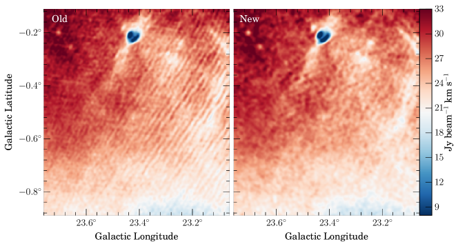
Figure 1: H i integrated intensity maps (in the velocity range $-100<v_{\rm LSR}<150$ km s^-1) for a sample region. The left panel shows the product in the THOR data release 1, which were obtained by direct feathering of the VLA C- and D-configuration observations with the GBT. The right panel shows the product in the THOR data release 2, which were obtained by combining the VLA C- and D-configuration data in the visibility domain and then feathering with the VGPS.

3 Results

We describe the parameters of the data products, and present an overview of the H i results in this section.

3.1 Data release 2

All spectral line data from the pilot and phase 1, as well as all Stokes I continuum data, have been published and are already available to the community (Bihr et al., 2015, 2016; Beuther et al., 2016, 2019; Walsh et al., 2016; Rugel et al., 2018; Wang et al., 2018). In this paper, we publish the data from the second half of the survey, including the new H I dataset for the whole survey, available at our project website and at the CDS. We summarize the basic parameters of the data products in Table 1. Because of different requirements for calibrating and imaging the polarization data (see also Beuther et al., 2016), the data reduction of these data for the whole survey is still ongoing. The first results of the Faraday rotation study in Galactic longitude range 39° to 52° are presented by Shanahan et al. (2019). More polarization data should be available at a later stage.

The noise of our data is dominated by the residual side lobes. Particularly in regions close to strong emission from the continuum and the masers, the noise can increase significantly. The noise properties of the continuum data and OH masers are studied in detail by Bihr et al. (2016), Beuther et al. (2016), Walsh et al. (2016), Wang et al. (2018), and Beuther et al. (2019). We list only the typical noise values in Table 1.

Table 1: Properties of the data products in the THOR data release 2.

	Rest Freq.	Width	$\Delta v$	beam	beam	noise
	(MHz)	(km s-1)	(km s-1)	native	smoothed	mJy beam-1
H I	1420.406	277.5	1.5	–	40″	10
H I+cont.	1420.406	300	1.5	13.0″ to 19.1″	25″	10
OH1	1612.231	195	1.5	11.6″ to 18.7″	20″	10
OH2	1665.402	195	1.5	11.1″ to 18.1″	20″	10
OH3	1667.359	195	1.5	11.0″ to 13.7″	20″	10
OH4	1720.530	195	1.5	11.0″ to 17.6″	20″	10
RRL	–	210	10	–	40″	3.0
cont1	1060	–	–	14.7″ to 24.4″	25″	1.0
cont2	1310	–	–	12.2″ to 19.7″	25″	0.3
cont3	1440	–	–	11.6″ to 18.1″	25″	0.3
cont4	1690	–	–	9.5″ to 15.4″	25″	0.3
cont5	1820	–	–	9.1″ to 14.5″	25″	0.3
cont6	1950	–	–	8.2″ to 13.1″	25″	0.7
cont3+VGPS	1420	–	–	–	25″	6.5

3.2 OH

Continuum subtracted images at both the native and the smoothed resolution (20″) of the four OH lines are provided to the community. The correlator setup was slightly different between the pilot study, phase 1, and phase 2, which mainly affects the sky coverage of OH lines and RRLs and the native spectral resolution of spectral lines (see Beuther et al. 2016 for details). The OH line at 1667 MHz was only observed in the pilot study and phase 2 ($l=29.2\degr-31.5\degr,\ 37.9\degr-47.9\degr$, and $51.1\degr-67.0\degr$, see also, Rugel et al. 2018 and Beuther et al. 2019).

Diverse physical processes are traced by OH masers, from expanding shells around evolved star to shocks produced by star-forming jets or SNRs (Elitzur, 1992). Beuther et al. (2019) survey identified 1585 individual maser spots distributed over 807 maser sites in the THOR survey, among which $\sim$50% of the maser sites are associated with evolved stars, $\sim 20$% are associated with star-forming regions, and $\sim 3$% are potentially associated with SNRs (see Beuther et al. 2019 for details).

Thermal OH lines are often detected as absorptions towards strong continuum sources, and they can be used to trace molecular clouds where CO is not detected, so called “CO-dark” regions (e.g., Allen et al., 2015; Xu et al., 2016). By studying the two main transitions (1665 and 1667 MHz), Rugel et al. (2018) detect 59 distinct OH absorption features against 42 continuum background sources, and most of the absorptions occur in molecular clouds associated with Galactic H ii regions. This is the first unbiased interferometric OH survey towards a significant fraction of the inner Milky Way, and provides a basis for theoretical and future follow-up studies (see Rugel et al. 2018 for details).

3.3 RRLs

As mentioned in the previous section, to increase the signal-to-noise (S/N), ratio we smoothed and stacked all available recombination line images. The final RRL images have an angular resolution of 40″ and a velocity resolution of 10 km s^-1. The typical linewidths of RRLs measured toward H ii regions are around $\sim 20-25$ km s^-1(Anderson et al., 2011), so a 10 km s^-1 resolution is reasonable to study the kinematics of H ii regions.

Combining the RRL data from THOR with complementary CO data, Rugel et al. (2019) found shell-like structures in RLL emission toward W49A. The ionized emission and molecular gas emission show correlation towards the shell-like structures. By comparing to one-dimensional feedback models (Rahner et al., 2017, 2019), Rugel et al. (2019) suggest W49A is potentially regulated by feedback-driven and re-collapsing shells (see Rugel et al. 2019 for details).

Mostly due to sensitivity limitations, interferometric mapping surveys of RRL emission have been rare (e.g., Urquhart et al., 2004). The stacking method allows us to achieve higher sensitivities than is usually possible when only single lines are observed. THOR provides the community with a new set of RRL maps towards a large sample of H ii regions, which can be used for sample statistical studies.

3.4 Continuum

As presented in Wang et al. (2018), the THOR survey provides the continuum data (both at the native resolution and smoothed to a resolution of 25″), as well as a continuum source catalog, to the community. To recover the extended structure, we combined the C-configuration 1.4 GHz continuum data from THOR with the 1.4 GHz continuum data from the VGPS survey (D+Effelsberg) using the task, “feather” (Wang et al., 2018). The resulting images for the pilot region and phase 1 are very similar to the ones obtained using the VGPS continuum as an input model in the deconvolution of the THOR data. This combined dataset retains the high angular resolution of the THOR observations (25″), and at the same time, it can recover the large-scale structure. Anderson et al. (2017) identified 76 new Galactic SNR candidates in the survey area with this dataset. Anderson et al. (2017) further showed that despite the different bandwidths between the VGPS continuum ($\sim 1$ MHz) and the THOR continuum ($\sim 128$ MHz), the flux retrieved from the combined data is consistent with the literature.

The continuum source catalog contains 10 387 objects that we extracted across our survey area. With the extracted peak intensities of the six usable SPWs between 1 and 2 GHz, we were able to determine a reliable spectral index (spectral index fitted with at least 4 SPWs) for 5657 objects. By cross-matching with different catalogs, we found radio counter parts for 840 H ii regions, 52 SNRs, 164 planetary nebulae, and 38 pulsars. A large percentage of the remaining sources in the catalog are likely to be extragalactic background sources, based on their spatial and spectral index distributions. A detailed presentation of the continuum catalog can be found in Bihr et al. (2016) and Wang et al. (2018).

3.5 H i

For the H i 21 cm line, in addition to the data cubes from C+D+GBT data, we also provide the C-configuration-only H i datacubes with continuum at both the native resolution and the smoothed beam (25″), which can be used to measure the H i optical depth towards bright background continuum sources (Bihr et al., 2016).

A case study of H i self-absorption towards a giant molecular filament is presented by Wang et al. (submitted). In the following sections, we focus scientifically on H i emission and absorption.

3.5.1 H i emission

Figure 2 shows the C+D+single-dish 1.4 GHz continuum map and the H i integrated intensity map ($v_{\rm LSR}=-113\sim 163$ km s^-1). While the combined H i emission data illustrates that the atomic gas is confined near the Galactic mid-plane at lower longitudes ($l<42\degr$), at larger longitudes ($l>54\degr$) gas is more evenly distributed in latitudes. The H i map in Fig. 2 also shows absorption patterns against some strong continuum sources, such as the star-forming complex W43 at $l\sim 30.75\degr$, and W49 at $l\sim 43\degr$.

Figure 3 depicts the channel maps by integrating the H i emission over 15 km s^-1 velocity bins. The neutral gas is clearly seen located at higher latitude in channels at $v_{\rm LSR}<-38$ km s^-1. This is likely due to the H i disk being strongly warped in the outer Milky Way (Burton & te Lintel Hekkert, 1986; Diplas & Savage, 1991; Nakanishi & Sofue, 2003; Kalberla & Kerp, 2009). Some cloud structures are more prominent in the channel maps, such as the filamentary structures in the channels at $v_{\rm LSR}<-38$ km s^-1. While at negative velocities the filamentary structures can been seen clearly, the emission at positive velocities appears less structured. This observational phenomenon is likely due to higher spatial and velocity crowding of structures at positive velocities. The negative velocity channels are tracing the outer Galactic plane, and there is little line of sight confusion, while at positive velocities, due to near-far distance ambiguity, the emission from multiple spiral arms could be at the same velocity and result in structures at different distances bing blended together.

The integrated intensity map (Fig. 2) also demonstrates that the angular size of the H i emission along the latitude is smaller at lower longitudes than at larger longitudes. This is due to the fact that the tangent points are further away at lower longitudes. This is also seen in the channel map (Fig. 3) in the positive velocities, in which the tangent points are traced by the left end of the emission in each panel with positive velocities, and the emission structures appear to be smaller at lower longitudes due to them being further away (see also, Merrifield, 1992).

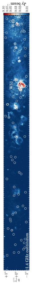
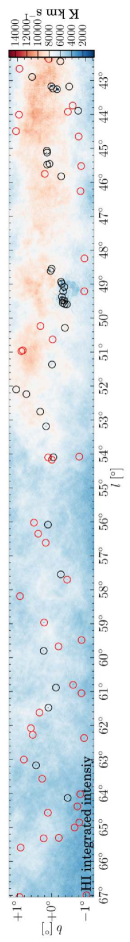
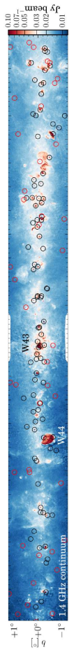
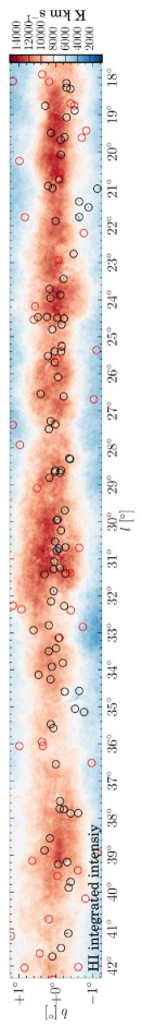
Figure 2: THOR+VGPS 1.4 GHz continuum map and H i integrated intensity map ($-113<v_{\rm{LSR}}<163$ km s^-1). The continuum map has a beam size of 25″, and the beam size for the H i map is 40″. In all panels, the circles mark the continuum sources that we used to extract the H i absorption spectra and construct the optical depth map (see Sect. 3.5.2). The Galactic sources are marked with white and black circles, and the extragalactic sources are marked with red circles. A few well-known Galactic sources are also labeled in each panel (W43 at $l\sim 31$°, W44 $l\sim 35$°, W49 $l\sim 43$°and W51 $l\sim 49$°).

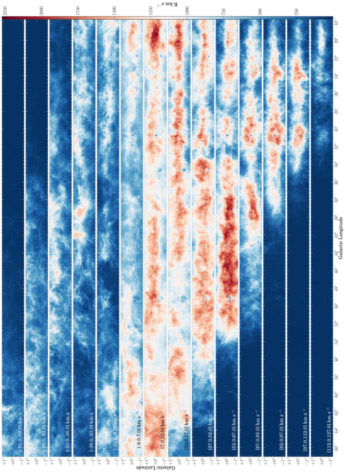
Figure 3: H i channel maps produced by integrating the H i emission over indicated velocity ranges. Strong absorption towards W43 ($l\sim 31$°), W44 ($l\sim 35$°), W49 ($l\sim 43$°) and W51 ($l\sim 49$°) are clearly visible across several velocity channels.

By averaging the emission in the latitude axis, we constructed the longitude-velocity ($l-v$) diagram of the H i emission (Fig. 4). The general shape of the $l-v$ diagram agrees with one obtained with the VGPS data (Strasser et al., 2007), but the higher resolutions reveal much finer details, such as the vertical lanes at $l\sim 31\degr,\ 43\degr$, and $\sim 49\degr$, which are caused by absorption against the background continuum emission from the star-forming regions W43, W49, and W51, respectively (see also Fig. 2). We also created the ¹³CO(1–0) $l-v$ diagram with the same method and plotted it as contours in Fig. 4. The ¹³CO(1–0) data is taken from the Exeter FCRAO CO Galactic Plane Survey (Mottram & Brunt, 2010), and Galactic Ring Survey (GRS, Jackson et al., 2006). We re-gridded the Exeter ¹³CO data to the same velocity resolution and coverage as the GRS, so there is no ¹³CO coverage at velocities where $v_{\rm LSR}<-5$ km s^-1. Compared to the ¹³CO emission, the H i emission also traces more extended and diffuse structures.

The H i emission in general agrees well with the spiral arm models of Reid et al. (2016), except for the Outer Scutum-Centaurus (OSC) Arm. The OSC Arm is at a large Galactocentric distance and is outside of our survey area at longitudes larger than 40° due to the warping and flaring of the outer disk (Dame & Thaddeus, 2011; Armentrout et al., 2017). Thus, we can only detect a small portion of the OSC Arm in the inner part of the Galactic plane that our survey covers, as illustrated in Fig. 4.

Another feature in the $l-v$ diagram is a strong self-absorption pattern at $\sim$5 km s^-1 following the Aquila Rift (magenta box in Fig. 4). This absorption feature spans almost 20° in longitude ($\sim$17° to 36°). The ¹³CO emission, on the other hand, lies right inside the absorption feature in the $l-v$ diagram. This large-scale absorption feature could be caused by the Riegel-Crutcher cloud, which centers at $v_{\rm LSR}\sim 5$ km s^-1 and covers the longitude range $l=345\degr$ to 25°, and the latitude range $b\leq 6\degr$ (Riegel & Jennings, 1969; Riegel & Crutcher, 1972; Crutcher & Riegel, 1974).

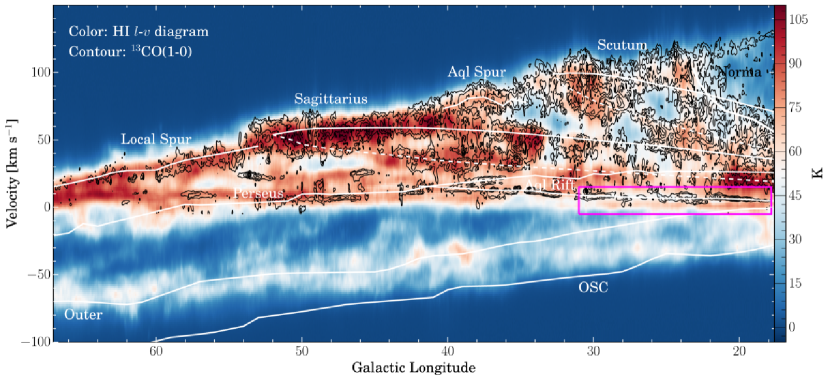
Figure 4: H i longitude-velocity ($l-v$) diagram constructed by averaging the emission in the latitude range $\lvert b\rvert\leq 1.25\degr$. The black contours correspond to the ¹³CO(1–0) $l-v$ at 3, 8, 18, 28, and 38 times the rms noise of the $l-v$ diagram (rms = 0.1 K, $T_{\rm MB}$). The ¹³CO(1–0) data do not cover the velocity range $v_{\rm LSR}<-5$ km s^-1. The overlaid curves trace the Sagittarius, Scutum, Norma, Perseus, Outer, and Outer Scutum-Centaurus (OSC) arms, and smaller features (Local Spur, Aquila Spur, and Aquila Rift) taken from Reid et al. (2016). The near and far sides of the arms are plotted with dashed and solid lines, respectively. The magenta box marks the absorption feature could be caused by the Riegel-Crutcher cloud. The ¹³CO(1–0) data are from the Exeter FCRAO CO Galactic Plane Survey (Mottram & Brunt, 2010), and the GRS (Jackson et al., 2006).

After resampling both the H i and ¹³CO data to the same angular and spectral resolution (pixel size of 22″, beam size of 46″, and velocity resolution of 1.5 km s^-1), we constructed the $T_{\rm B}$(H i)/$T_{\rm B}$(¹³CO) ratio $l-v$ diagram by dividing the H i $l-v$ diagram by the ¹³CO $l-v$ diagram (Fig. 5). For the ¹³CO $l-v$ diagram, a 3$\sigma$ value was used where the emission is below 3$\sigma$ (1$\sigma=0.04$ K in the ¹³CO $l-v$ diagram). As expected, Fig. 5 shows that the $T_{\rm B}$(H i)/$T_{\rm B}$(¹³CO) ratio is low where there is ¹³CO emission (see also, Sect 4.3).

After removing the pixels with no H i emission ($T_{\rm B}$(H i)$<5\sigma$, 1$\sigma$=0.2 K), the histogram of the $T_{\rm B}$(H i)/$T_{\rm B}$(¹³CO) ratio $l-v$ diagram in Fig. 6 reveals one strong peak at $\sim 100,$ and a secondary peak at $\sim 600$. If we assume both H i and ¹³CO emissions are optically thin and uniform excitation temperature, the variations in the $T_{\rm B}$(H i)/$T_{\rm B}$(¹³CO) ratio also represent the variations in the atomic to molecular gas column density ratio. Figure 6 indicates that the atomic-to-molecular gas column density ratio can increase by a factor of six from inter-arm regions to spiral arms. Considering that we used 3$\sigma$ value of the ¹³CO $l-v$ diagram for regions where there is no ¹³CO emission to construct the $T_{\rm B}$(H i)/$T_{\rm B}$(¹³CO) ratio $l-v$ diagram, this factor of six is a lower limit (see also Sect 4.3).

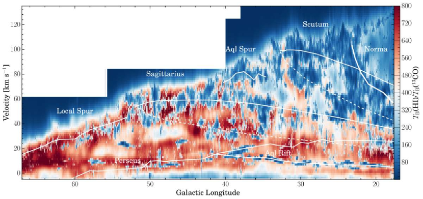
Figure 5: The ratio map $l-v$ diagram of H i over ¹³CO ($T_{\rm B}$(H i)/$T_{\rm B}$(¹³CO)) averaged over galactic latitude. The ¹³CO(1–0) data do not cover the velocity range $v_{\rm LSR}<-5$ km s^-1. The overlaid curves trace the Sagittarius, Scutum, Norma, Perseus, Outer, and Outer Scutum-Centaurus (OSC) arms, and smaller features (Local Spur, Aquila Spur, and Aquila Rift) taken from Reid et al. (2016). The near and far sides of the arms are plotted with dashed and solid lines, respectively.

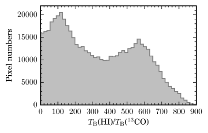
Figure 6: Histogram of the $T_{\rm B}$(H i)/$T_{\rm B}$(¹³CO) ratio $l-v$ diagram shown in Fig. 5.

3.5.2 H i optical depth

The THOR C-configuration-only H i data (Beuther et al., 2016), which have not been continuum-subtracted, are used to measure the H i optical depth towards bright background continuum sources. We extracted the H i spectra towards all continuum sources with an S/N ratio larger than seven from Wang et al. (2018). Since the synthesized beam of the C-configuration-only H i data is 25″, we extracted the average H i spectrum from a $28\arcsec\times 28\arcsec$ ($7\times$7 pixels) area centered on the position of the continuum source to increase the S/N ratio. We used the software STATCONT (Sánchez-Monge et al., 2018) to estimate the continuum level $T_{\rm cont}$ and the noise of the spectra. Some example spectra are shown in Fig. 7. With the absorption spectra, we can estimate the optical depth towards the continuum source following the method described in Bihr et al. (2015):

$$\tau=-{\rm ln}\left(\frac{T_{\rm{on,\ cont}}-T_{\rm off,\ cont}}{T_{\rm{cont}}}\right),$$ (1)

where $T_{\rm on,\ cont}$ is the brightness temperature of the absorption feature measured towards the continuum source, and $T_{\rm off,\ cont}$ is the off-continuum-source brightness temperature. Since we use the THOR C-configuration data to calculate $\tau$, the smooth, large-scale structure is mostly filtered out (Beuther et al., 2016). Therefore, we can neglect the off emission $T_{\rm off,\ cont,}$ and simplify Eq. 1 to:

$$\tau_{\rm{simplified}}=-{\rm ln}\left(\frac{T_{\rm{on,\ cont}}}{T_{\rm{cont}}}\right).$$ (2)

For channels with a $T_{\rm{on,\ cont}}$ value less than three times the rms, we use the 3$\sigma$ value to get a lower limit on $\tau$. The bottom panels in Fig. 7 show the $\tau$ spectra for the corresponding sources, and the calculated $\tau$ is always saturated in some channels. Compared to the VGPS VLA D-configuration absorption spectra and the $\tau$ spectra derived from them (resolution 60″, Strasser et al. 2007), the THOR C-configuration absorption spectra are much more sensitive and therefore probing higher optical depth (Fig. 7).

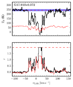
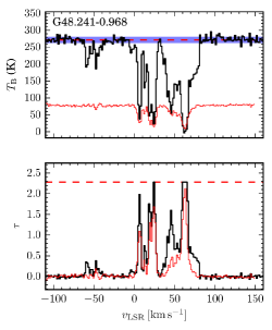
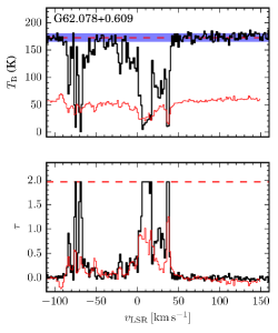
Figure 7: H i absorption and optical depth ($\tau$) spectra of THOR (thick black spectra) and VGPS (thin red spectra). The dashed lines mark the continuum level $T_{\rm cont}$ in the top panels, and the lower limit of $\tau$ in the bottom panels. The shaded bands in the top panels mark the 1$\sigma$ level of the noise.

In this study, since only $T_{\rm{on,\ cont}}<(T_{\rm cont}-3\leavevmode\nobreak\ \sigma$) is considered to be real absorption, only sources with $T_{\rm cont}>6\leavevmode\nobreak\ \sigma$ can have channels with real absorption and do not reach the lower limit of $\tau$. In total, 228 sources have a $T_{\rm cont}>6\leavevmode\nobreak\ \sigma$ to make the $\tau$ map, among which $\sim$60% are Galactic sources (Table LABEL:table_tau). We listed $T_{\rm cont}$, $\sigma$ of $T_{\rm cont}$, the lower limit of $\tau$, and the integrated $\tau$ including the physical nature of the 228 sources in Table LABEL:table_tau. We then grid the 228 $\tau$ measurements channel by channel for the whole survey using the nearest-neighbor method to create the $\tau$ data-cube. Since the Galactic sources do not trace any absorption from the gas located behind them, we replaced the optical depth values for these channels with the ones from the nearest extragalactic sources. The resulting integrated $\tau$ map is shown in Fig. 8.

The highest integrated $\tau$ we measured is at $l\sim 43$°, at the location of the high-mass star-forming complex W49A. A very high integrated $\tau$ is measured towards the star-forming complex W43 ($l\sim 31$°). Figure 8 shows that higher $\tau$ is measured in the inner longitude range, which is reasonable considering more material is packed along the line of sight due to velocity crowding in regions below $l\sim 43$°. Since the used $\tau$ spectra are all saturated in some channels, this map represents a lower limit of the optical depth in the survey region.

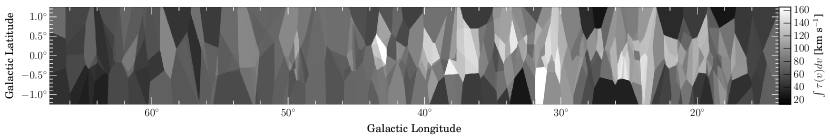
Figure 8: H i integrated optical depth ($\tau$) map across the velocity range ($-128.5<v_{\rm LSR}<$170 km s^-1). The aspect ratio of the figure is modified for demonstration purpose.

3.5.3 H i column density and distribution

We estimated the column density of atomic hydrogen from the emission line data (C+D+GBT) using (e.g., Wilson et al., 2013):

$$N_{\rm H}=1.8224\times 10^{18}\>\int T_{\rm S}(v)\tau(v)\,dv.$$ (3)

The optical depth corrected spin temperature is $T_{\rm S}(v)=T_{\rm B}(v)/(1-{\rm e}^{-\tau(v)})$, where $T_{\rm B}$ is the brightness temperature of the H i emission. We used the $\tau$ data-cube (Sect. 3.5.2) to correct the spin temperature channel by channel and estimate the column density.

As shown in Fig. 2 and Fig. 3, H i absorption against strong continuum sources is clearly seen as negative features in the continuum subtracted emission map, such as toward W43 at $l\sim 31\degr$. To derive the column density toward strong continuum sources, we determined a mean brightness temperature from a region of radius 10 ′ around the continuum source to derive $T_{\rm S}$. Then, we extracted C-configuration-only H i+continuum spectra from these regions pixel-by-pixel to derive the optical depth (see Sect. 3.5.2). With the spin temperature and optical depth derived, we can estimate the column density towards continuum sources and add these to the optical depth corrected column density map. Figure 9 shows the histograms of the atomic hydrogen column density integrated between –113 to 163 km s^-1 of the survey area. The median value of the column density is 1.8$\times 10^{22}$ cm^-2, which is 38% higher than the value assuming optically thin emission.

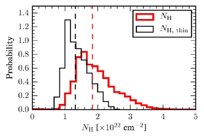
Figure 9: Histograms of the atomic hydrogen column density integrated between –113 to 163 km s^-1. The black (thin) histogram represents the column density derived assuming the emission is optically thin, and the red (thick) histogram represents the column density corrected fro optical depth. The dashed vertical lines mark the median values of the two histograms, respectively.

To obtain the distribution of atomic gas in the Galactic plane, we estimated the kinematic distance of each channel and each pixel of the H i emission map with the Kinematic Distance Utilities (Wenger et al., 2018). The “universal” rotation curve of Persic et al. (1996) including terms for an exponential disk and a halo, as well as the Galactic parameters from Reid et al. (2014) are used. See Table. 5 in Reid et al. (2014) for detailed parameters.

To solve the kinematic distance ambiguity in the inner Galaxy (inside the solar orbit), we took the following approach. We assume that the average vertical density profile of the atomic gas $n(z)$ in the inner Galaxy can be described by the sum of two Gaussians and an exponential function (Lockman, 1984; Dickey & Lockman, 1990):

$$\begin{split}n(z)=\ &\sum_{i=1}^{2}n_{i}(0)\ {\rm exp}\ \left[-z^{2}/\left(2h_{i}^{2}\right)\right]\\ &+n_{3}(0)\ {\rm exp}\ \left(-|z|/h_{3}\right),\end{split}$$ (4)

with $z$ describing the distance from the Galactic mid-plane. The coefficients from Dickey & Lockman (1990) are listed in Table 2. Since the volume density distribution of the atomic gas in the mid-plane is approximately axisymmetric with respect to the Galactic center (Kalberla & Dedes, 2008), we can assume the volume density is the same at the same Galactocentric distance in the mid-plane. Furthermore, the $v_{\rm LSR}$ distance profiles are symmetric with respect to the tangent point for the degeneracy part (see also, Anderson & Bania, 2009), so each velocity bin traces the same line-of-sight distance at the near side as at the far side. Thus we assume the column density is also the same at the same Galactocentric distance at the near and far side in the Galactic mid-plane. Due to the kinematic distance ambiguity in the inner Galaxy, the column density we derived for each pixel at each velocity channel is a combined result from both the far and near side. Thus, we can use Eq. 4 to estimate the percentage of the column density contribution from the near and far side for each line-of-sight to solve the kinematic distance ambiguity.

Table 2: Coefficients of Eq. 4 taken from Dickey & Lockman (1990).

i	$n_{i}(0)$ (cm-3)	$h_{i}$ (pc)
1	0.395	90
2	0.107	225
3	0.064	403

With the kinematic distances determined for each channel, we applied a 5$\sigma$ cut and converted the column density cube into a face-on mean surface density map, shown in Fig. 10. Comparing to the spiral arm model from Reid et al. (2016), some of the atomic gas follows the spiral arms well, such as the Sagittarius and Perseus arms, but there is also much atomic gas in the inter-arm regions. Along the Sagittarius and Perseus arms, and in the very outer region beyond the Outer Arm in Fig. 10, the H ii region distribution agrees with the atomic gas. However, the Outer Arm itself is not associated with much atomic gas in the face-on plot, although there is good agreement between the H I emission and the Outer Arm in the $l-v$ diagram. This outer component of the atomic gas was also observed by Oort et al. (1958), Nakanishi & Sofue (2003), and Levine et al. (2006). Nakanishi & Sofue (2003) found this emission structure agrees spatially with the Outer Arm discovered by Weaver (1970). The Perseus Arm and Outer Arm in Fig. 10 are found to be distinct structures in the atomic gas distribution with a void of H i emission and H ii regions between the arms. The absolute value of the derived surface density represents a mean surface density along the $z$ direction, and is therefore lower than the results of Nakanishi & Sofue (2003) and Nakanishi & Sofue (2016), which derived a surface density integrated along $z$.

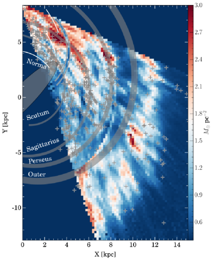
Figure 10: Face-on view of H i surface mass distribution in the survey area overlaid with spiral arms from Reid et al. (2016), and H ii regions from Anderson et al. (2014). The Galactic center is at $\left[0,\leavevmode\nobreak\ 0\right]$, and the Sun is at the top-left corner at a Galactocentric distance of 8.34 kpc (Reid et al., 2014). The gray lanes mark the Outer, Perseus, Sagittarius, and Scutum arms with widths from Reid et al. (2014). The Local Spur, Aquila Spur, and Norm Arm are marked with white lines. The long bar (Hammersley et al., 2000; Benjamin et al., 2005; Nishiyama et al., 2005; Benjamin, 2008; Cabrera-Lavers et al., 2008) is marked with the shaded half-ellipse. The crosses mark the H ii regions from Anderson et al. (2014) excluding the ones that fall into the tangent region (marked with two gray curves).

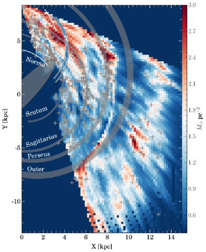
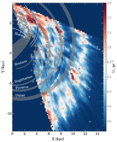
Figure 13: Face-on view of the H i surface mass distribution produced with different kinematic distance determination methods. Left panel: Kinematic distances were determined with IAU Solar parameters ($R_{0}=8.5$ kpc, $\Theta_{0}=220$ km s^-1) and Galactic rotation model from Brand & Blitz (1993). Right panel: Kinematic distances were determined with the Galactic parameters from Reid et al. (2014) with a uniform Galactic rotation curve. The rest of the symbols are the same as Fig. 10

We applied different Galactic models and rotation curves for the kinematic distance determination to create the face-on surface density maps shown in Fig. 13. We find that the face-on density map depends only slightly on the assumed model for the kinematic distance. Compared to Fig. 10 (Galactic parameters from Reid et al. 2014, rotational curve from Persic et al. 1996), the assumption of a uniform rotational curve (Fig. 13, right) only lowers the gas surface density close to the bar region. Similar changes occur when applying the IAU Solar parameters ($R_{0}=8.5$ kpc, $\Theta_{0}=220$ km s^-1) and the Brand & Blitz (1993) Galactic rotation model (Fig. 13, left), together with slightly shifting the gas to higher distances.

3.5.4 Mean spin temperature of the atomic gas

With the H i emission, we can obtain the line-of-sight mean spin temperature or the density-weighted harmonic mean spin temperature using (Dickey et al., 2000):

$$\left<T_{\rm S}\right>=\frac{\int T_{\rm B}(v)\ dv}{\int 1-e^{-\tau(v)}\ dv}.$$ (5)

As we show in Fig. 11, the mean spin temperatures in the THOR survey area are between 50 and 300 K, with a median value of 143 K. We do not see any correlation between $\left<T_{\rm S}\right>$ and longitudes. Combining survey data from VGPS (Stil et al., 2006), CGPS (Taylor et al., 2003), and SGPS (McClure-Griffiths et al., 2005), Dickey et al. (2009) studied the atomic gas in the outer disk of the Milky Way (outside the solar circle). They found the mean spin temperature to be $\sim$250–400 K, and it stays nearly constant with the Galactocentric radius to $\sim$25 kpc. Since the mean spin temperature $\left<T_{\rm S}\right>$ reveals the fraction of CNM in the total atomic gas (see Equation 8 in Dickey et al. 2009), the lower $\left<T_{\rm S}\right>$ we obtained indicates we observe a higher fraction of CNM in our survey area. Since Dickey et al. (2009) only considered the outer Milky Way, the differences in the $\left<T_{\rm S}\right>$ may indicate a higher fraction of CNM in the inner Milky Way.

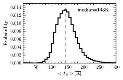
Figure 11: Histograms of density-weighted harmonic mean spin temperature between –113 to 163 km s^-1. The dashed vertical lines mark the median values of 143 K.

4 Discussion

We discuss the results of H i overview presented in Sect. 3 in this section.

4.1 H i gas mass

With the method described in Sect. 3.5.3, we estimate the optical depth corrected total H i mass in our survey area to 4.7$\times 10^{8}\leavevmode\nobreak\ M_{\odot}$ (using emission above 5$\sigma$). Combining ¹²CO(1–0) and ¹³CO(1–0) from the GRS and the Exeter FCRAO CO Survey, Roman-Duval et al. (2016) estimated an H₂ mass in the inner Galaxy (inside the solar circle) of 5.5$\times 10^{8}\leavevmode\nobreak\ M_{\odot}$ (GRS: $18\degr\leq l\leq 55.7\degr$, —$b\leq 1\degr$—; Exeter: $55\degr\leq l\leq 100\degr$, $-1.4\leq b\leq 1.9\degr$). Within the solar circle, we estimate the total H i mass to be 2.1$\times 10^{8}\leavevmode\nobreak\ M_{\odot}$ ($18\degr\leq l\leq 67\degr$, —$b|\leq 1.25\degr$). Although the GRS+Exeter survey covers a larger area than THOR, the area they covered inside the solar circle is only $\sim 4\%$ larger than THOR, so we can still compare these two masses. Therefore, in the inner Galaxy in this longitude range, the molecular component represents about 72% of the total gas. This fraction also agrees with the molecular fraction of 50-60% of total gas inside the solar circle estimated by Koda et al. (2016), Nakanishi & Sofue (2016), and Miville-Deschênes et al. (2017). Considering the total H i mass we derived is a lower limit, this percentage is likely an upper limit.

If we assume the H i emission to be optically thin, the total H i mass within the whole survey area is estimated to be $3.6\times 10^{8}\leavevmode\nobreak\ M_{\odot}$. Comparing this with our optical-depth corrected estimate of 4.7$\times 10^{8}\leavevmode\nobreak\ M_{\odot}$, we find that the mass increases by $\sim$31% percent with the optical depth correction. Considering that all of the $\tau$ spectra saturate in some channels, this $31\%$ is again a lower limit. We define the ratio between the mass after and before the optical depth correction as $R_{\rm{H\textsc{I}}}$, so for the whole survey area $R_{\rm{H\textsc{I}}}=1.31$. Assuming optically thin emission, the total mass of the H i gas of the Milky Way within the Galactic radius of 30 kpc was estimated to be 7.2–8$\times 10^{9}\leavevmode\nobreak\ M_{\odot}$ (Kalberla & Kerp, 2009; Nakanishi & Sofue, 2016). If we apply $R_{\rm{H\textsc{I}}}=1.31$ to the whole Milky Way, the total H i gas mass would be 9.4–10.5$\times 10^{9}\leavevmode\nobreak\ M_{\odot}$. We discuss the uncertainties of the total H i mass in Sect. 4.5.

As part of the pilot study of the THOR project, Bihr et al. (2015) estimated the mass of the atomic hydrogen gas in the W43 region after applying the correction for optical depth and absorption against the diffuse continuum emission and derived an $R_{\rm{H\textsc{I}}}=2.4$, which is higher than what we have derived for the entire survey. Considering W43 has the second largest integrated $\tau$ in the survey, it is reasonable that a larger than average $R_{\rm{H\textsc{I}}}$ was measured here. The optical depth map (Fig. 8) also shows higher $\tau$ in the inner longitude region ($l\lesssim 44\degr$) than in the outer longitude region.

In contrast to this, Lee et al. (2015) found $R_{\rm{H\textsc{I}}}\sim 1.1$ by applying the optical depth correction pixel-by-pixel towards the atomic gas around the Perseus molecular cloud. Combining the 21 cm emission maps from the Galactic Arecibo L-band Feed Array Survey (GALFA-HI Peek et al., 2011, 2018) and absorption spectra from 21-SPONGE (Murray et al., 2015, 2018b), Murray et al. (2018a) found $1.0<R_{\rm{H\textsc{I}}}<1.3$ towards high latitude local ISM ($|b|>15\degr$). Considering that we are observing with much higher angular resolution than GALFA, and multiple spiral arms along the line of sight are at the same velocity in the Galactic plane, it is reasonable that the $R_{\rm{H\textsc{I}}}$ we derived is higher. On the other hand, studies toward nearby galaxies (M31, M33 and LMC) found $R_{\rm{H\textsc{I}}}\sim 1.3-1.34$ (Braun et al., 2009; Braun, 2012), which is in agreement with what we found.

4.2 H i gas distribution

Ever since van de Hulst et al. (1954) and Oort et al. (1958) discovered the spiral structure of the atomic hydrogen gas in the Milky Way, considerable effort has been devoted to investigating the gas distribution and spiral arms in the Galaxy (e.g., Kulkarni et al., 1982; Nakanishi & Sofue, 2003; Levine et al., 2006; Kalberla & Kerp, 2009; Nakanishi & Sofue, 2016). The structure outside of the Outer Arm in Fig. 10 was also observed by Oort et al. (1958), Nakanishi & Sofue (2003), Levine et al. (2006), and Nakanishi & Sofue (2016). Nakanishi & Sofue (2003) fit this structure with the so-called Outer Arm with a pitch angle of $\sim 7\degr$ in the polar coordinates (the x-axis is the azimuthal angle $\theta$ and the y-axis the Galactic radius $R$ in log scale). They found that this agrees with the Outer Arm found by Weaver (1970). Also, one of the arms fit by Levine et al. (2006) goes through the northern part of this structure (Y $>0$, X $>10$ in Fig. 10). Levine et al. (2006) claimed that the spiral arm model derived from the H ii regions (Morgan et al., 1953; Georgelin & Georgelin, 1976; Wainscoat et al., 1992) could not fit this structure, although Fig. 10 shows that many H ii regions are associated with this structure. The Outer Arm plotted in Fig. 10 is extrapolated from the pitch angle fitted to parallax sources at greater longitudes ($l>70\degr$, Reid et al., 2016). Since the pitch angle can vary by azimuth angle (Honig & Reid, 2015), the real Outer Arm in this region ($17\degr<l<67\degr$) could have a different pitch angle and be at a larger Galactocentric radius. On the other hand, the noncircular motions in the outer H i disk (e.g., Kuijken & Tremaine, 1994) could also affect the H i distribution we derived in this region.

Another feature in the inner part of Fig. 10 is that the region right below the end of the bar shows low surface density. Depending on the Galactic rotation model we used to determine the kinematic distances, there could even be a cavity in this region (all emission is below 5$\sigma$ and masked out, Fig. 13). The region is located where the Galactic long bar ends (Hammersley et al., 2000; Benjamin et al., 2005; Nishiyama et al., 2005; Benjamin, 2008; Cabrera-Lavers et al., 2008). The long bar introduces strong non-circular motions in the sources, and so the axisymmetric rotation curve does not apply on and near the bar (Fux, 1999; Rodriguez-Fernandez & Combes, 2008; Reid et al., 2014). Thus, the kinematic distances derived for the gas and most H ii regions in this region may have large errors. Therefore, the low-level emission may not be real. The same low-level distribution is also seen in the CO map by Roman-Duval et al. (2009, 2016), in H ii regions. Considering all these distributions are based on kinematic distance (except for the distance of less than 10% H ii regions in this region are derived from parallax), we should consider the distribution of gas and H ii regions inside Scutum Arm with caution.

4.3 Atomic to molecular gas ratio

Our optical depth correction discussed in the previous sections involves a lot of interpolation and averaging. We would like to avoid doing it when comparing the H i and ¹³CO maps, since interpolation and averaging brings large uncertainties to each particular region. In the following discussion, we compare the H i and ¹³CO emission directly.

As we demonstrate in Fig. 10, high column density gas is concentrated along and above the Sagittarius Arm in the inner Galaxy. This is also seen by Nakanishi & Sofue (2016). On the other hand, molecular clouds traced by CO are mainly distributed around and inside the Scutum Arm (Roman-Duval et al., 2009; Nakanishi & Sofue, 2016). The molecular cloud fraction ($f_{\rm mol}$) map in Nakanishi & Sofue (2016) shows that $f_{\rm mol}$ is anti-correlated with Galactocentric distance. Compared to Fig. 10, inside the Sagittarius Arm, the molecular cloud fraction may be as high as $f_{\rm mol}>0.6$, while in the outer regions, $f_{\rm mol}$ quickly drops to almost zero (see also, Miville-Deschênes et al., 2017). However, they did not discuss how this ratio varies between inter-arm regions and spiral arm regions.

As the $l-v$ diagrams in Fig. 4 and Fig. 5 show that the majority of the molecular gas is tightly associated with the spiral arms, while the atomic gas on the other hand is more widely distributed with significant material in the inter-arm regions. The histogram of $T_{\rm B}$(H i)/$T_{\rm B}$(¹³CO) ratio shows a bimodal distribution (Fig. 6). If we assume both ¹³CO and H i emissions are optically thin, the $T_{\rm B}$(H i)/$T_{\rm B}$(¹³CO) ratio bimodal distribution could be proxy of the atomic-to-molecular gas ratio. Therefore, we can interpret from Fig. 6 that on average, the atomic-to-molecular gas ratio may increase by approximately a factor of six from spiral arms to inter-arm regions.

4.4 Uncertainties of the H I optical depth $\tau$

The uncertainties of the H i optical depth are determined mainly by two factors, the brightness of the continuum source and the rms noise of the absorption spectra. The ratio of these two is the S/N ratio. As we mentioned in Sect. 3.5.2, we selected sources with an S/N ratio $>$6 to ensure that the spectra have real absorption and the $\tau$ spectra is not saturated in all channels. Thus, the S/N ratio for the selected spectra ranges between six and 250, with a median value of 12, and the uncertainties associated with the rms noise are between 0.18 to 0.004 with a median value of 0.09, depending on the brightness of the continuum source.

Another source of uncertainty for the optical depth $\tau$ is that the $\tau$ spectra are all saturated in some channels, as shown in Fig. 7. To test the $\tau$ limits, high sensitivity VLA follow-up observations were carried out towards three selected sources, G21.347–0.629, G29.956–0.018, and G31.388–0.384 (Rugel et al., in prep.). In the THOR survey, where each field was observed for five to six minutes in on-source time, the optical depths of these three sources all saturate at $\tau\sim$2.7 to 3.1. In the follow-up observations, each continuum source was observed for significantly longer, and the noise dropped by $\sim 50-70\%$. However, many channels in the $\tau$ spectra still saturate at $\tau\sim 3.5-3.9$ if we smooth the data to the same angular and spectral resolution as the THOR C-configuration data. Depending on the S/N ratio of the continuum source, this $\sim 50-70\%$ drop in the noise could increase the lower limit of the optical depth to $\sim 1.2-2.6$ times the current value, and also increase the optical-depth corrected column density to $\sim 1.1-1.6$ times the current value (Fig. 12).

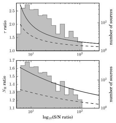
Figure 12: Increase of the optical depth lower limit (top panel) and the column density (bottom panel) if the noise drops by 50% (dashed line) and 70% (solid line) plotted as a function of S/N ratio. The shaded histogram in each panel is the S/N ratio distribution of the continuum sources we used to extract the H i absorption spectra and construct the optical depth map.

4.5 Uncertainties of the H I mass

The uncertainties of the mass estimation for atomic gas originate from several factors: the optical depth, the distance, absorption against the diffuse continuum emission, and the H i self absorption (HISA). As we discussed in the previous section, we could be underestimating the peak optical depth $\tau_{\rm limit}$ by 20 to 160%, but the impact on the integrated optical depth is not clear. If we assume the noise levels of the $\tau$ spectra drop to 30% of the values listed in Table. LABEL:table_tau, with the same 228 sources to correct the optical depth, the total H I mass increases by 9%. However, as we mentioned in the previous section, many channels in the $\tau$ spectra still saturate in the high sensitivity follow-up observations, and this 20% is still a lower limit.

The second main factor of uncertainty is the distance. With different Galactic parameters, we get different kinematic distances, which result in different mass estimates. With the rotation curve of Persic et al. (1996), and the Galactic parameters from Reid et al. (2014), we derived the total mass 4.7$\times 10^{8}M_{\odot}$. With the same Galactic parameters from Reid et al. (2014) but assuming a uniform rotational curve, we would get the same mass. If we take the IAU Solar parameters ($R_{0}=8.5$ kpc, $\Theta_{0}=220$ km s^-1) and Galactic rotation model from Brand & Blitz (1993), the total mass increases by 13%. We are also aware that assuming axisymmetry and using the average vertical density distribution $n(z)$ of H i to solve the kinematic distance ambiguity of the column density distribution is not ideal, but this is the best we can do without detailed modeling of the Galactic disk. Furthermore, Wenger et al. (2018) compared the kinematic distances with the parallax distances of 75 Galactic high-mass star-forming regions, and they found out that the kinematic distances we used in this paper (derived with the rotation curve of Persic et al. (1996) and the Galactic parameters from Reid et al. (2014)) have a median offset of 0.43 kpc, with a standard deviation of 1.24 kpc from parallax distances.

Bihr et al. (2015) estimated the mass of the atomic hydrogen gas in W43 to be $6.6_{-1.8}\times 10^{6}\leavevmode\nobreak\ M_{\odot}$ after applying the correction for optical depth and absorption against the diffuse continuum emission ($l=29.0-31.5\degr,\ |b|\leq 1\degr,\ v_{\rm LSR}=60-120$ km s^-1). By integrating across the same velocity range, we derived a mass of 8.5$\times 10^{6}\leavevmode\nobreak\ M_{\odot}$ within the same area with our distance determination method. The mean distance at $l=30.25\degr$ between 60 to 120 km s^-1 from our method is 7.4 kpc, much larger than the distance of 5.5 kpc (Zhang et al., 2014) adopted by Bihr et al. (2015). Taking the same distance 5.5 kpc results in a mass of $4.9\times 10^{6}\leavevmode\nobreak\ M_{\odot}$. Further applying correction for the absorption against the diffuse continuum emission with the method described in Bihr et al. (2015) increases the mass by 19% to $5.7\times 10^{6}\leavevmode\nobreak\ M_{\odot}$, which approximately agrees with what Bihr et al. (2015) estimated, but is slightly smaller. Since Bihr et al. (2015) use one single strong continuum source to correct the optical depth for the whole W43 region, they may overcorrect for the outer region in W43. The 19% mass increase from applying a correction for the absorption against the diffuse continuum emission is an upper limit if we consider the whole survey area, since W43 is one of the most extreme star-forming complexes in the Milky Way and is considered to be a mini starburst region (Nguyen-Lu’o’ng et al., 2011; Beuther et al., 2012; Nguyen-Lu’o’ng et al., 2013; Zhang et al., 2014). Furthermore, to correct the diffuse continuum emission, we need information on its distance. It is reasonable to assume all diffuse continuum emission is in the background and correct it for a particular region, but we can not apply this to the whole survey. Thus, we do not apply any correction for the diffuse continuum emission.

The last factor is HISA, which we did not consider for the mass estimation. However, HISA was studied towards a Giant Molecular Filament (GMF) with the THOR data by Wang et al., submitted, and they showed, for this specific GMF, that the mass traced by HISA is only 2-4% of the total H i mass. Studies of H i narrow self absorption (HINSA) show that the ratio between the column density traced by HINSA to the H₂ column density is $\sim 10^{-3}$ to $2\times 10^{-2}$ (Li & Goldsmith, 2003; Goldsmith & Li, 2005; Zuo et al., 2018). As we discussed in Sect. 4.1, the total H₂ mass in this part of the Galactic plane is also comparable to the H i mass, the effect of HISA and HINSA to the H i mass is negligible. In summary, we could still be underestimating the H i mass by 20 to 40%, even with the current optical depth correction.

5 Conclusions

In this paper, we describe the THOR data release 2, which includes all OH and RRL data, and an entire new H i dataset from the THOR survey. In addition, a detailed analysis of the H i data is presented. The main results can be summarized as follows:

1. While the H i channel map shows clear filamentary substructures at negative velocities, the emission at positive velocities is more smeared-out. This is likely due to higher spatial and velocity crowding of structures at positive velocities. Both the $l-v$ diagram and the face-on view of the H i emission show that some of the atomic gas follows the spiral arms well, such as the Sagittarius and Perseus Arm, but there is also much gas in the inter-arm regions.

2. We produced a spectrally resolved H i $\tau$ map from 228 absorption spectra.

3. We corrected optical depth for the H i emission with the $\tau$ map. The atomic gas column density we derived with optical depth correction is 38% higher than the column density derived with optically thin assumption. We estimate the total H i mass in the survey region to be 4.7$\times 10^{8}\leavevmode\nobreak\ M_{\odot}$, 31% higher than the mass derived with the optically thin assumption. If we apply this 31% correction to the whole Milky Way, the total atomic gas mass would be 9.4–10.5$\times 10^{9}\leavevmode\nobreak\ M_{\odot}$.

4. Considering that all the $\tau$ spectra are saturated in some channels and we did not apply the correction for the diffuse continuum emission, we could be underestimating the mass by an additional 20–40%. Future higher sensitivity observations are needed to better constrain the optical depth.

5. We constructed a face-on view of the mean surface density of the atomic gas in the survey area.

6. We estimated the density-weighted harmonic mean spin temperature $\left<T_{\rm S}\right>$ integrated between –113 and 165 km s^-1 with a median value of $\left<T_{\rm S}\right>\sim 143$ K, about a factor of two lower than what was estimated in the outer disk of the Milky Way, which may indicate a higher fraction of CNM in the inner Milky Way.

7. The latitude averaged $T_{\rm B}$(H i)/$T_{\rm B}$(¹³CO) ratio distribution shows two peaks at $\sim$100 and $\sim$600, which may indicate that the atomic-to-molecular gas ratio can increase by a factor of six from spiral arms to inter-arm regions.

The H i, OH, RRL, and continuum data from the THOR survey together provide the community the basis for high-angular-resolution studies of the ISM in different phases.

Appendix A Optical depth measurements towards the selected sources

1]

Table 3: Optical depth measurements towards the selected continuum sources.

Gal.ID	$T_{\rm cont}$	rms	$\tau_{\rm limit}$	$\int\tau(v)dv$	$R_{\rm eff}$	Note
	(K)	(K)		(km s-1)	″
G14.490+0.021	117	17	0.8	30	22	HII
G15.035–0.677	4286	17	4.4	33	289	HII
G15.168+0.797	134	13	1.2	28	23
G15.190–0.596	244	20	1.4	17	111	HII
G15.913+0.183	97	16	0.7	16	74	SNR_green
G16.557+0.453	99	13	0.9	26	19
G16.733–1.185	218	23	1.1	26	21	Xray
G16.784–1.058	162	16	1.2	23	40	jet
G16.945–0.074	114	12	1.1	59	30	HII
G17.910+0.372	244	11	2.0	53	21
G18.092+1.167	145	20	0.9	15	22
G18.106+0.186	179	12	1.6	65	24
G18.148–0.283	462	15	2.3	40	99	HII
G18.270–0.289	110	15	0.9	16	184	HII
G18.303–0.390	542	13	2.6	43	32	HII
G18.696–0.401	97	14	0.8	40	20
G18.755–0.497	83	10	1.0	54	19
G18.761+0.287	106	17	0.7	26	252	SNR_green
G18.886–0.508	120	14	1.1	26	145	HII
G19.075–0.287	281	15	1.8	45	223	HII
G19.432–0.824	79	13	0.7	25	20
G19.492+0.135	223	14	1.7	76	100	HII
G19.610–0.235	889	15	3.0	80	112	HII
G19.621–0.701	70	10	0.9	25	19
G19.679–0.131	153	17	1.1	55	45	HII
G20.080–0.136	145	13	1.3	67	33	HII
G20.252+0.991	119	14	1.0	24	23
G20.594–0.130	109	13	1.0	66	18
G20.750–0.090	89	13	0.8	35	175	HII
G20.923+0.213	89	15	0.7	21	23	Xray
G20.989+0.090	195	11	1.8	56	62	HII
G20.999–1.125	126	19	0.8	13	26	PN
G21.347–0.629	521	12	2.7	55	23	Xray
G21.503–0.884	1095	14	3.2	36	58	SNR_green
G21.765–0.631	129	12	1.3	38	313	SNR_green
G21.770+0.843	131	14	1.1	21	21
G21.874+0.008	288	13	2.0	80	31	HII
G22.199–0.756	90	13	0.8	28	25
G22.760–0.478	109	14	1.0	17	100	HII
G22.933–0.076	117	19	0.7	55	28	jet;Xray
G23.438–0.209	228	13	1.7	69	166	HII
G23.710+0.171	275	13	1.9	68	59	HII
G23.871–0.121	266	11	2.1	86	51	HII
G23.956+0.150	595	16	2.5	51	56	HII
G24.180+0.565	253	17	1.6	66	25
G24.463+0.245	120	14	1.1	75	166	HII
G24.471+0.488	614	16	2.6	41	90	HII
G24.493–0.038	150	19	1.0	36	76	HII
G24.507–0.223	207	18	1.4	48	120	HII
G24.541+0.600	130	13	1.2	54	19
G24.675–0.154	254	20	1.5	62	71	HII
G24.798+0.096	354	17	1.9	57	152	HII
G25.237–0.150	240	15	1.6	91	46	jet
G25.266–0.161	325	15	1.9	99	21	Xray
G25.361–1.102	186	22	1.0	15	23
G25.395+0.033	190	18	1.2	73	48	HII
G25.397–0.141	1035	16	3.1	70	159	HII
G25.520+0.216	138	18	1.0	41	22	HII
G25.604–0.038	206	11	1.9	103	21
G25.692+0.031	114	10	1.3	64	77	HII
G26.090–0.058	122	14	1.1	63	127	HII
G26.544+0.414	345	13	2.2	50	73	HII
G26.609–0.212	93	14	0.8	37	21	HII
G26.687–1.028	123	14	1.1	14	22
G27.279+0.145	239	12	1.9	81	56	HII
G27.365+0.014	110	12	1.2	31	127	SNR_green
G27.380+1.167	131	19	0.8	10	29	jet
G27.494+0.190	186	15	1.4	60	112	HII
G27.920+0.977	364	17	2.0	23	25
G28.287–0.364	194	16	1.4	25	23	HII
G28.305–0.387	151	16	1.1	24	44	HII
G28.608+0.018	127	15	1.0	50	55	HII
G28.610–0.142	131	13	1.2	56	76	SNR_green
G28.652+0.027	125	18	0.8	35	67	HII
G28.672–0.108	134	13	1.2	53	63	SNR_green
G28.807+0.175	246	17	1.6	41	53	HII
G29.089+0.511	199	10	1.9	61	20
G29.689–0.242	607	20	2.3	52	100	SNR_green
G29.935–0.053	544	12	2.7	70	115	HII
G29.956–0.018	876	18	2.8	69	61	HII
G30.234–0.138	282	13	2.0	95	20	HII
G30.534+0.021	278	19	1.6	80	38	HII
G30.687–0.260	196	16	1.4	58	102
G30.699–0.630	148	16	1.1	59	29	jet
G30.720–0.083	192	12	1.7	62	15	HII
G30.782–0.027	1669	27	3.0	80	226	HII
G31.070+0.050	152	13	1.3	88	38	HII
G31.242–0.110	244	18	1.5	86	31	HII
G31.279+0.064	140	17	1.0	36	25	HII
G31.388–0.384	768	11	3.1	110	21
G31.394–0.259	142	17	1.0	48	56	HII
G31.412+0.307	401	24	1.7	48	27	HII
G31.869+0.064	410	19	1.9	50	193	SNR_green
G32.151+0.133	265	17	1.6	33	35	HII
G32.265+1.168	265	29	1.1	38	23
G32.272–0.226	153	15	1.2	48	28	HII
G32.363+0.934	162	16	1.3	52	30	jet
G32.389–0.403	208	13	1.7	50	20
G32.798+0.191	687	15	2.7	71	40	HII
G32.835–0.730	81	13	0.7	9	21
G32.928+0.607	133	11	1.4	60	29	HII
G33.133–0.093	92	12	0.9	42	28	HII
G33.143–0.066	98	12	1.0	58	22	jet
G33.417–0.004	88	13	0.8	30	55	HII
G33.498+0.194	484	9	2.8	103	20	Xray
G33.810–0.189	107	12	1.1	53	26	HII
G33.915+0.110	350	16	2.0	62	30	HII
G34.133+0.471	260	12	2.0	61	30	HII
G34.256+0.146	1343	17	3.2	66	83	HII
G34.568–0.630	78	11	0.8	18	153	SNR_green
G34.588–0.238	107	13	1.0	14	127	SNR_green
G35.053–0.518	92	14	0.8	26	85	HII
G35.139–0.762	105	16	0.8	11	30	HII
G35.467+0.139	130	16	1.0	37	23	HII
G35.574+0.068	193	16	1.4	55	27	HII
G35.947+0.379	93	11	1.0	50	22
G36.056+0.357	246	11	2.0	82	26	jet
G36.060+0.994	91	14	0.8	25	18
G36.516–0.970	95	12	1.0	27	20
G36.551+0.002	476	10	2.7	94	21	Xray
G37.545–0.112	272	14	1.9	84	59	HII
G37.750–0.107	92	12	1.0	46	45	HII
G37.763–0.215	426	13	2.4	85	71	HII
G37.868–0.601	118	13	1.1	47	19	HII
G37.874–0.399	833	12	3.1	103	39	HII
G38.549+0.163	67	10	0.8	33	25	HII
G38.875+0.308	97	12	1.0	52	21	HII
G38.932–1.126	79	13	0.7	18	21
G39.157+0.643	93	11	1.0	46	18
G39.187–0.303	108	13	1.0	49	171	SNR_green
G39.251–0.066	272	14	1.9	84	75	HII
G39.414–0.595	155	12	1.5	69	23
G39.565–0.040	258	11	2.1	91	19
G39.728–0.398	94	12	1.0	41	37	HII
G39.883–0.346	106	8	1.5	65	20	HII
G40.180–0.798	111	9	1.4	52	18
G40.733+0.192	106	9	1.3	57	20
G41.117–0.334	293	12	1.9	38	120	SNR_green
G41.189+1.221	117	18	0.8	27	17
G41.513–0.141	107	12	1.1	38	53	HII
G41.660+0.441	75	12	0.8	28	17
G41.741+0.097	137	12	1.4	53	21	HII
G42.028–0.605	213	10	1.9	61	21
G42.050+0.853	97	10	1.2	46	20
G42.365+0.079	59	9	0.7	33	20	jet
G42.434–0.260	131	10	1.4	44	65	HII
G42.653+0.946	102	12	1.1	36	21
G42.895+0.573	307	10	2.3	74	26	Xray
G43.171+0.007	2751	17	4.0	115	141	HII
G43.177–0.519	111	9	1.4	51	38	HII
G43.238–0.045	243	14	1.8	83	23	HII
G43.257–0.161	779	14	2.9	75	142	SNR_green;HII
G43.738–0.620	168	10	1.8	54	22
G43.890–0.783	152	11	1.5	41	40	HII
G43.921–0.479	120	14	1.1	45	28
G44.006+0.959	69	11	0.8	27	18
G44.492+1.045	110	13	1.0	32	21
G44.649–0.795	92	9	1.2	46	25	jet
G45.067+0.138	122	11	1.3	32	35	HII
G45.122+0.132	738	10	3.2	49	60	HII
G45.454+0.059	1172	11	3.6	59	133	HII
G45.478+0.130	544	12	2.7	55	63	HII
G45.519–0.870	117	9	1.5	47	22
G45.751+0.198	111	9	1.5	52	18
G45.823–0.284	103	10	1.2	32	48	HII
G46.260–0.851	78	9	1.1	37	19
G48.241–0.968	272	9	2.3	50	19
G48.545–0.003	79	10	1.0	37	45	HII
G48.610+0.027	126	13	1.1	43	97	HII
G48.930–0.280	494	17	2.3	39	120	HII
G48.983–0.299	201	15	1.5	41	74	HII
G49.079–0.374	350	17	1.9	41	87	HII
G49.206–0.342	943	20	2.8	44	107	HII
G49.210–0.963	376	14	2.2	44	30	jet
G49.370–0.302	1428	26	2.9	54	144	HII
G49.477–0.328	465	16	2.3	43	32	HII
G49.488–0.380	3600	27	3.8	61	163	HII
G49.553–0.330	74	11	0.8	23	32	HII
G49.586–0.385	365	16	2.0	37	66	HII
G49.594–0.449	89	15	0.7	13	50	HII
G50.234+0.327	212	13	1.7	61	32	jet
G50.285–0.392	100	12	1.0	38	31	HII
G50.626–0.031	206	11	1.8	48	19
G50.948+0.847	114	12	1.1	46	21
G50.970+0.890	85	12	0.9	40	20
G51.364–0.014	107	10	1.2	29	104	SNR_anderson
G52.099+1.042	206	12	1.7	34	26	HII
G52.236+0.742	71	10	0.9	24	103	HII
G52.753+0.334	168	11	1.6	46	27	HII
G53.185+0.161	144	12	1.4	46	77	HII
G54.078–0.813	87	9	1.2	37	22
G54.096–0.054	68	8	1.0	28	91	HII
G54.102+0.100	89	8	1.3	48	18
G54.170–0.009	152	11	1.5	44	20
G56.023+0.519	68	8	1.1	29	18
G56.082+0.105	154	7	1.9	42	20	Xray
G56.348+0.394	149	9	1.7	52	23
G56.616+0.170	56	8	0.8	23	19
G57.547–0.272	133	11	1.4	37	54	HII
G57.701–0.456	69	6	1.3	41	17
G58.189+0.931	62	9	0.8	23	19
G58.966+0.220	195	9	2.0	62	33	jet
G59.483–0.881	156	9	1.8	46	17
G59.672–0.206	51	7	0.8	27	17
G59.801+0.231	78	8	1.1	30	71	HII
G60.804–0.632	74	10	0.9	25	44	jet
G60.883–0.130	133	11	1.4	19	37	HII
G61.050–0.880	79	8	1.3	31	21
G61.475+0.092	1442	13	3.6	34	73	HII
G61.619+0.356	103	7	1.6	43	19
G62.078+0.609	173	8	2.0	48	20
G62.272+0.555	78	7	1.3	39	17
G62.366–0.956	570	13	2.7	36	35	jet
G63.002+0.817	294	8	2.5	41	19
G63.169+0.457	106	8	1.4	27	123	HII
G63.566+0.277	95	8	1.4	31	18
G64.019–0.846	113	9	1.4	19	18
G64.131–0.472	191	9	2.0	23	62	HII
G64.382–0.757	114	8	1.6	25	18
G64.567+0.107	163	11	1.6	47	24	jet
G64.854–0.814	73	10	0.9	16	21
G65.002–0.675	106	9	1.3	21	19
G65.307–0.214	327	9	2.5	38	19
G65.321+0.232	133	11	1.4	33	22
G65.594+0.911	113	9	1.4	33	19
G66.997–1.026	84	8	1.2	24	18
G67.051+0.942	85	9	1.1	49	18
G67.170+0.127	118	9	1.5	31	19

Table 3: continued.

Appendix B Face-on surface density maps of the atomic gas