Next-to-leading power threshold factorization for Drell-Yan production

Abstract:

We present the next-to-leading power (NLP) factorization formula for the $q\bar{q}\to\gamma^{*}+X$ channel of the Drell-Yan production near the kinematic threshold limit. The formalism used for the computation of next-to-leading power corrections within soft-collinear effective field theory is introduced, we discuss the emergence of new objects, the NLP collinear functions, and define them through an operator matching equation. We review the leading power factorization before extending it to subleading powers. We also present the one-loop result for the newly introduced collinear function, and demonstrate explicitly conceptual issues in performing next-to-leading logarithmic resummation at next-to-leading power.

1 Introduction

A detailed description of the soft-collinear factorization for the Drell-Yan (DY) process in the kinematic threshold limit at subleading powers has recently been presented in [1]. With this in mind, the aim of this contribution is to focus on the key ideas and results while keeping the technical details and subtleties to a minimum as much as it is possible. For these, we encourage the interested reader to consult [1] and [2].

The partonic process we consider is $q\bar{q}\to\gamma^{*}(Q)+X$ at threshold, that is the $z=Q^{2}/\hat{s}\to 1$ limit, where $\hat{s}=x_{a}x_{b}\,s$ is the partonic centre-of-mass energy squared, $x_{a},x_{b}$ are the momentum fractions of the partons inside the incoming hadrons and $Q^{2}$ is the invariant mass squared of the off-shell photon. The final state QCD radiation $X$ is forced to be soft and the cross-section is expanded in powers of $(1-z)$. The main results of this work, [1], and [2] are first, the derivation of the factorization formula at next-to-leading power (NLP) in the threshold expansion, and second, the identification of new physical objects that emerge beyond leading power: the amplitude level NLP collinear functions and, in addition, the generalized soft functions previously defined in [3].

Recently, interest in subleading-power corrections has arisen in the theoretical community. Subleading-power effects are important to consider both from a theoretical and a phenomenological perspective, in order to advance the understanding of all-order structure of quantum field theories, and improve subtraction methods. Computations of subleading-power corrections contribute to providing precise predictions for processes within the Standard Model (SM) and they can be numerically important. This was recently shown in the study of the leading logarithmic NLP corrections in Higgs prouction via gluon fusion [4]. These considerations are crucial in matching the experimental efforts, in particular in the upcoming era of HL-LHC. The conceptual leap to next-to-leading logarithmic accuracy at NLP is key as current efforts to extend the subleading power resummation beyond the leading logarithmic order have been hampered by the issue of endpoint divergences in ill-defined convolutions [1, 5, 6, 7, 8]. We make this issue explicit by considering the results of the computations presented here.

2 SCET formalism

In this work, the position-space formulation [9, 10] of soft-collinear effective theory (SCET) [11, 12, 13] is used. The SCET Lagrangian is split into $N$ collinear sectors, denoted by a subscript $c_{i}$, which interact with each other only through the exchange of soft partons. Namely, it is given by

$$\mathcal{L}_{{\rm{SCET}}}=\sum^{N}_{i=1}\,\mathcal{L}_{c_{i}}+\mathcal{L}_{{\rm{soft}}}\,,$$ (1)

where each of the Lagrangians belonging to a collinear direction is expanded in powers of the small power-counting parameter $\lambda$. In the present case the small power-counting parameter is $\lambda=\sqrt{1-z}$ which corresponds to the threshold-collinear scale:

$$\,\mathcal{L}_{c_{i}}=\underbrace{\mathcal{L}^{(0)}_{c_{i}}}_{\rm{LP}}+\underbrace{\mathcal{L}^{(1)}_{c_{i}}}_{\mathcal{O}(\lambda^{1})}+\underbrace{\mathcal{L}^{(2)}_{c_{i}}}_{\mathcal{O}(\lambda^{2})}+\,\,...$$

The first term in this expansion constitutes the leading power (LP) contribution, and the terms which follow are the subleading-power corrections. This formalism can in general describe $N$-jet processes. In the case of the DY production we set $N=2$, resulting in collinear, $c$, and anticollinear, $\bar{c}$, sectors. The LP collinear Lagrangian is given by [10]

$${\mathcal{L}}^{(0)}_{c}=\bar{\xi}_{c}\left(in_{-}D_{c}+g_{s}\,{\color[rgb]{1,0,0}n_{-}A_{s}(z_{-})}+i\not{D}_{\perp c}\frac{1}{in_{+}D_{c}}\,i\not{D}_{\perp c}\right)\frac{\not{n}_{+}}{2}\,\xi_{c}+\mathcal{L}^{(0)}_{c,{\rm{YM}}}\,,$$ (2)

with $in_{-}D_{c}=in_{-}\partial+g_{s}\,{\color[rgb]{0,0,1}n_{-}A_{c}(z)}$. $\mathcal{L}^{(0)}_{c,{\rm{YM}}}$ is the LP soft-collinear Yang-Mills Lagrangian, the unspecified arguments of collinear fields are the full $z$ coordinates, $n^{\mu}_{-},n^{\mu}_{+}$ are light-like vectors with $n_{-}\cdot n_{+}=2$, and ${\color[rgb]{1,0,0}A_{s}}$ is evaluated at position $z_{-}^{\mu}=(n_{+}z){n_{-}^{\mu}}/{2}$ as a consequence of multipole expansion. The soft-collinear interaction at LP is given by the standard eikonal vertex.

Importantly, at LP, we can apply the decoupling transformation [12], for example for the initial state collinear quark: $\xi_{c}(z)\to Y_{+}(z_{-})\,\xi_{c}^{(0)}(z)$, where

$$Y_{\pm}\left(x\right) = \mathbf{P}\exp\left[ig_{s}\int_{-\infty}^{0}ds\,n_{\mp}A_{s}\left(x+sn_{\mp}\right)\right],$$ (3)

is the soft Wilson line. This field redefinition removes all the interactions between the soft and collinear fields from the LP Lagrangian in (2) as

$$\bar{\xi}_{c}\,(in_{-}D_{c}+g_{s}{\color[rgb]{1,0,0}n_{-}A_{s}(x_{-})})\,\frac{\not{n}_{+}}{2}\,\xi_{c}=\bar{\xi}_{c}^{(0)}\,in_{-}D_{c}^{(0)}\,\frac{\not{n}_{+}}{2}\,\xi_{c}^{(0)}\,,$$ (4)

where the superscript $(0)$ denotes the decoupled fields.

We next consider the SCET formalism beyond the leading power. The systematic expansion in powers of $\lambda$ which is built into the SCET framework means that this effective field theory is ideally suited to the study of power corrections. The formalism we use here was developed in [3, 14, 15, 16]. A generic, $N$-jet, operator has the following form

$$J=\int dt\,C(\{t_{i_{k}}\})J_{s}(0)\prod_{i=1}^{N}J_{i}(t_{i_{1}},t_{i_{2}},...).$$ (5)

It is a product of $N$ operators, $J_{i}$, each of which associated with a particular collinear direction, and a soft operator, $J_{s}$, which consists only of soft fields. The measure is given by $dt=\prod_{{ik}}dt_{i_{k}}$ and $C(\{t_{i_{k}}\})$ is a hard matching coefficient. Each of the $J_{i}$ operators is constructed from collinear-gauge-invariant collinear building blocks

$$J_{i}(t_{i_{1}},t_{i_{2}},...)=\prod_{k=1}^{n_{i}}\psi_{i_{k}}(t_{i_{k}}n_{i+})\,,$$ (6)

which are given by

$$\psi_{i}(t_{i}n_{i+})\in\,\left\{\begin{array}[]{ll}\displaystyle\chi_{i}(t_{i}n_{i+})\equiv W_{i}^{\dagger}\,\xi_{i}&\quad{\rm{collinear\,quark}}\\[8.5359pt] \displaystyle\mathcal{A}^{\mu}_{i\perp}(t_{i}n_{i+})\equiv W_{i}^{\dagger}\left[i\,D^{\mu}_{i\perp}\,W_{i}\right]&\quad{\rm{collinear\,gluon}}\end{array}\right.$$ (7)

Each of the building blocks scales as $\mathcal{O}(\lambda)$. In the above equation, we make use of the i^th-collinear Wilson line, which is a path-ordered exponential of $n_{i+}A_{i}$. For DY, we require $i=c$ which is given by

$$W_{c}\left(x\right) = \mathbf{P}\exp\left[ig_{s}\int_{-\infty}^{0}ds\,n_{+}A_{c}\left(x+sn_{+}\right)\right],$$ (8)

and a corresponding definition for the $\bar{c}$-direction with $n_{+}\leftrightarrow n_{-}$.

The LP configuration is simply given by the presence of one building block in each of the $N$ collinear directions,

$$J^{A0}_{i}(t_{i})=\psi_{i}(t_{i}n_{i+}).$$ (9)

There is a number of ways to include power suppression in this formalism. The first, is to introduce derivatives, $\partial^{\mu}_{\perp}\sim\lambda$, that act on the fields present in the LP configuration. The second way, is to place additional building blocks in a particular collinear direction, each building block gives a power of $\lambda$ suppression. This procedure gives rise to subleading power currents such as ${\color[rgb]{0.76953125,0,0.390625}J^{An}_{i}},{\color[rgb]{0,0.4296875,0.75}J^{Bn}_{i}},{\color[rgb]{0,0.65234375,0.3125}J^{Cn}_{i}}$. They are labelled as follows:

• ${\color[rgb]{0.76953125,0,0.390625}A},{\color[rgb]{0,0.4296875,0.75}B},{\color[rgb]{0,0.65234375,0.3125}C}...$ refers to number of fields in a given collinear direction

• $n$ is the power of $\lambda$ suppression (relative to $A0$) in a given sector.

Examples of such currents are

$${\color[rgb]{0.76953125,0,0.390625}i\partial^{\mu}_{\perp i}i\partial^{\nu}_{\perp i}\chi_{i}},\hskip 11.38092pt{\color[rgb]{0,0.4296875,0.75}\chi_{i}(t_{i_{1}})i\partial^{\nu}_{\perp i}\mathcal{A}^{\mu}_{i\perp}(t_{i_{2}})},\hskip 11.38092pt{\color[rgb]{0,0.65234375,0.3125}\chi_{i}(t_{i_{1}})\chi_{i}(t_{i_{2}})\mathcal{A}^{\mu}_{i\perp}(t_{i_{3}})},\hskip 11.38092pt$$

for ${\color[rgb]{0.76953125,0,0.390625}J^{A2}_{i}},{\color[rgb]{0,0.4296875,0.75}J^{B2}_{i}},$ and ${\color[rgb]{0,0.65234375,0.3125}J^{C2}_{i}}$ respectively. The overall power suppression for the $N$-jet operator is given by the sum of the power suppression from the different sectors. Hence, an $\mathcal{O}(\lambda^{2})$ 2-jet operator could be given by the following

$$J^{A2}_{1}J^{A0}_{2},\hskip 28.45274ptJ^{A1}_{1}J^{B1}_{2},\hskip 28.45274ptJ^{A0}_{1}J^{C2}_{2},\,\,...$$

In addition to the currents described above, there is also the possibility to form time-ordered products of subleading-power Lagrangian terms with lower power currents in order to provide power suppression. These contributions, ${\color[rgb]{0.8671875,0.2890625,0.171875}J^{Tn}_{i}}$, are labelled by the letter $T$ and a number $n$ which gives the total power suppression from the current and the insertions of the subleading-power Lagrangian terms. An example is

$${\color[rgb]{0.8671875,0.2890625,0.171875}J^{T2}_{i}(t_{i_{1}})=i\int d^{4}z\,\mathbf{T}\big{[}\chi_{i}(t_{i_{1}})\mathcal{L}^{(2)}_{i}(z)\big{]}},$$ (10)

where $\mathcal{L}^{(2)}_{i}(z)$ is a $\lambda^{2}$ power-suppressed Lagrangian term [10]. These time-ordered product insertions play a crucial role the derivation of the factorization formula for the threshold DY production at NLP, and we will investigate them in much greater detail in the later sections.

3 Factorization at leading power

Having briefly introduced the subleading-power SCET formalism we turn our attention to the specific case of the DY process at threshold. We will first review the LP factorization, and later investigate the subleading-power effects. The partonic DY proccess at threshold is described by a standard SCET_I set up. In terms of the power-counting parameter $\lambda$, defined above, the threshold-collinear modes are given by

$${\color[rgb]{0,0,1}p_{c}} = (n_{+}p_{c},n_{-}p_{c},p_{c\perp})\sim Q(1,\lambda^{2},\lambda),$$

$${\color[rgb]{0.0,0.6,0.0}p_{\bar{c}}} = (n_{+}p_{\bar{c}},n_{-}p_{\bar{c}},p_{{\bar{c}}\perp})\sim Q(\lambda^{2},1,\lambda),$$

$${\color[rgb]{1,0,0}p_{s}} = (n_{+}p_{s},n_{-}p_{s},p_{s\perp})\sim Q(\lambda^{2},\lambda^{2},\lambda^{2}).$$ (11)

In addition to these modes, at hadronic level there exist the (anti)collinear-PDF modes, with the transverse momentum scaling of $p_{\perp}\sim\Lambda$, where $\Lambda$ is the scale of strong interactions. The $c$-PDF modes have momentum scaling $(Q,\Lambda^{2}/Q,\Lambda)$. The usual parton distribution functions (PDFs) are described by these modes. Here we consider the power corrections in $\lambda$ and work at leading power in $\Lambda$. The set up is perturbative as the threshold-collinear scale is still much larger than the scale of strong interactions $\Lambda$, $Q\lambda=Q\sqrt{(1-z)}\gg\Lambda$.

The first step in the derivation of factorization of DY in SCET at LP [22] involves matching the electromagnetic quark current to the LP SCET current,

$$\bar{\psi}\gamma_{\rho}\psi(0)=\int dt\,d\bar{t}\,\widetilde{C}^{A0,A0}(t,\bar{t}\,)\,J_{\rho}^{A0,A0}(t,\bar{t}\,)$$ (12)

where in our notation ($A0$ labelling the LP currents in the collinear and anticollinear directions)

$$J_{\rho}^{A0,A0}(t,\bar{t}\,)=\bar{\chi}_{\bar{c}}(\bar{t}n_{-})\gamma_{\perp\rho}\chi_{c}(tn_{+})\,$$ (13)

before the decoupling transformation [12] is used. The calculation proceeds by taking the matrix element of the above operator for the incoming (anti)collinear (anti)quark and the final state QCD radiation, $X$. Performing now the decoupling transformation, the states factorize and one obtains

$$\langle X|\bar{\psi}\,\gamma^{\,\rho}\psi(0)|A(p_{A})B(p_{B})\rangle = \int dt\,d\bar{t}\,C^{A0,A0}(t,\bar{t}\,)\,\langle X^{{\rm PDF}}_{\bar{c}}|\bar{\chi}_{\bar{c}}\,(\bar{t}n_{-})|B(p_{B})\rangle\,\gamma_{\perp}^{\,\rho}$$ (14)

$$\times\,\langle X^{{\rm PDF}}_{{c}}|\chi_{c}\left(tn_{+}\right)|A(p_{A})\rangle\,\langle X_{s}|{\mathbf{T}}\left(\left[Y_{-}^{\dagger}(0)Y_{+}(0)\right]\right)|0\rangle\,.$$

A picture of the factorization at amplitude level is presented in Fig. 1. We note here that the final state radiation can be soft, $X_{s}$ and PDF-collinear, $X^{{\rm PDF}}_{{c}}$, but not threshold-collinear. This is an important point, to which we will return to below. However, in the LP calculation the usual steps follow. Upon squaring of the above matrix element, performing the sum over the final state radiation, and combining the hadronic result with the lepton tensor gives the following

$$\frac{d\sigma_{\rm DY}}{dQ^{2}}=\frac{4\pi\alpha_{\rm em}^{2}}{3N_{c}Q^{4}}\sum_{a,b}\int_{0}^{1}dx_{a}dx_{b}\,f_{a/A}(x_{a})f_{b/B}(x_{b})\,\hat{\sigma}^{{\,\rm{LP}}}_{ab}(z)\,.$$ (15)

The $f_{a/A}(f_{b/B})$ is the standard PDF formed by the square of the (anti)collinear matrix element in (14). The focus of our investigations is the perturbative factorization of the LP partonic cross section. At LP, the partonic cross section $\hat{\sigma}^{{\,\rm{LP}}}_{ab}(z)$ factorizes into a hard function, originating from squaring the hard matching coefficient $C^{A0,A0}(t,\bar{t}\,)$ and a soft function:

$$\hat{\sigma}^{{\,\rm{LP}}}(z)=H(Q^{2})\,QS_{\rm DY}(Q(1-z))\,.$$ (16)

The leading power DY soft function is given by the vacuum matrix element of only the soft Wilson lines [23]

$$S_{\rm DY}(\Omega)=\int\frac{dx^{0}}{4\pi}\,e^{i\Omega\,x^{0}/2}\,\frac{1}{N_{c}}\,\mbox{Tr}\,\langle 0|\mathbf{\bar{T}}(Y^{\dagger}_{+}(x^{0})Y_{-}(x^{0}))\,\textbf{T}(Y^{\dagger}_{-}(0)Y_{+}(0))|0\rangle\,.$$ (17)

Before starting the discussion of extending this factorization formula to subleading powers, we would like to draw attention to the simplicity of the LP result in (16). There is no collinear dynamics present and the result is simply a product of the hard function and one soft function.

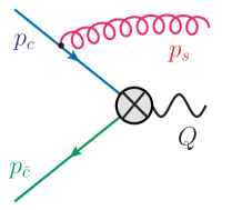
(a) Amplitude representation prior to use of decoupling transformation.

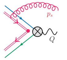
(b) Schematic representation after decoupling transformation is performed.

Figure 1: Representation of the LP amplitude before and after the decoupling transformation.

4 Factorization at next-to-leading power

Thus far we have reviewed the LP factorization which is already well established in the literature [24, 22]. In this section we take the step beyond, which is to consider the factorization of the partonic cross section at NLP. We denote this contribution by $\hat{\sigma}^{{\rm{NLP}}}_{ab}(z)$ and it replaces $\hat{\sigma}^{{\rm{LP}}}_{ab}(z)$ in Eq. (15). We will first present the result in a schematic way since we wish to highlight the new features that are present. In the following sections we will motivate their appearance and write down their precise form.

We begin by stating that the NLP partonic cross section is given by

$$\hat{\sigma}^{{\,\rm{NLP}}}=\sum_{\rm{terms}}\,[C\otimes{\color[rgb]{0,0,1}J}\otimes{\color[rgb]{0.0,0.6,0.0}\bar{J}}\,\,]^{2}\otimes{\color[rgb]{1,0,0}S}\,,$$ (18)

where $C$ is the hard Wilson matching coefficient, ${\color[rgb]{1,0,0}S}$ is a generalized soft function and ${\color[rgb]{0,0,1}J}$ is a NLP collinear function. The sum over “terms” means the sum over all the possible ways of inducing power suppression in the partonic cross section. Let us now motivate the emergence of this structure at next-to-leading power.

4.1 NLP collinear functions

The first obvious difference in the schematic NLP cross section in (18) with respect to the LP result in (16) is the presence of the amplitude level NLP collinear functions, ${\color[rgb]{0,0,1}J}$. These are indeed a new physical feature of the factorization starting at NLP. We would like to first explain why these collinear functions have not played a part in the derivation of the LP factorization formula and the reason for their appearance here. A detailed argument has been presented in [1] and here we outline the main ideas.

Figure 2: Insertion of the power-suppressed Lagrangian $\mathcal{L}^{(2)}_{2\xi}$ into a collinear quark line, which transforms a $c$-PDF quark into a threshold-collinear quark.

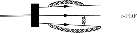
Figure 3: The loops depicted in the figure have threshold-collinear scaling. However, since at LP the matrix element does not have support for these modes, they can be trivially integrated out, $\chi_{c}\to{\chi}^{{\rm PDF}}_{c}$.

The key observation at LP is that the decoupling transformation completely removes the soft-collinear interactions in the LP Lagrangian as was stressed in Sec. 2. Therefore, diagrams such as the one presented in Fig. 2 do not feature in the calculations. This means that in the on-shell matching to the $c$-PDF fields, loops formed only by the threshold-collinear fields can appear. These are scaleless and therefore zero to all orders in perturbation theory in dimensional regularization. This is represented in Fig. 3. Hence, in practice, the threshold-collinear modes are trivially integrated out and the threshold-collinear fields are simply identified with $c$-PDF fields, $\chi_{c}\to{\chi}^{{\rm PDF}}_{c}$. For this reason, we have not discussed collinear functions in the derivation of the LP factorization formula between equations (14) and (15). The collinear functions are in fact present there, but they are delta functions to all orders in perturbation theory:

$$\chi_{c}(tn_{+})=\int\,du\,\tilde{J}(t,u)\,\chi_{c}^{\rm{PDF}}(un_{+})$$ (19)

with the collinear function written in position space $\tilde{J}(t,u)=\delta(t-u)$. Therefore, as stated, the computation proceeds in the usual way: the square of collinear matrix elements forms the PDFs  in (15).

The considerations are different when we start to investigate the NLP corrections. The ultimate reason for this is the presence of the time-ordered product operators, $J^{Tn}$, which can be used to provide power suppression as mentioned in Sec. 2. Insertions of the subleading-power Lagrangian terms introduce multiple threshold-collinear fields into the problem with an integral over the position of the insertion. The soft fields from the Lagrangian insertions are evaluated at the multipole expanded position. This means that there is an extra convolution between the soft and collinear sectors which makes the threshold-collinear loops non-vanishing. We make these statements more concrete through the following example.

We consider a term from the subleading-power Lagrangian

$$\mathcal{L}^{(2)}_{2\xi}(z)=\frac{1}{2}\,\bar{\chi}_{c}(z)\,z^{\mu}_{\perp}\,z^{\nu}_{\perp}\,\Big{[}i\partial_{\nu}\,in_{-}\partial\,\mathcal{B}^{+}_{\mu}(z_{-})\Big{]}\frac{\not{n}_{+}}{2}\,\chi_{c}(z).$$ (20)

The $\chi_{c}$ fields are the decoupled fields with the superscript $(0)$ dropped and

$$\mathcal{B}_{\pm}^{\mu} = Y_{\pm}^{\dagger}\left[i\,D^{\mu}_{s}\,Y_{\pm}\right]\,,$$ (21)

is the gauge invariant soft gauge field. We stress that the decoupling transformation has already been performed and the soft-collinear interactions persist, as is clear from the Lagrangian term. The NLP analogue of equation (14) in this example is the following

$$\langle X|\bar{\psi}\gamma^{\rho}\psi(0)|A(p_{A})B(p_{B})\rangle = \int dt\,d\bar{t}\,C^{A0,A0}(t,\bar{t}\,)\,\langle X^{{\rm PDF}}_{\bar{c}}|\bar{\chi}_{\bar{c},\alpha a}(\bar{t}n_{-})|B(p_{B})\rangle\gamma_{\perp,\alpha\gamma}^{\rho}$$ (22)

$$\times\,i\int d^{4}z\,\langle X^{{\rm PDF}}_{{c}}|\frac{1}{2}z_{\perp}^{\nu}z_{\perp}^{\mu}(in_{-}\partial_{z})^{2}\,\mathbf{T}\left[\chi_{c,\gamma f}\left(tn_{+}\right)\bar{\chi}_{c}\left(z\right)\textbf{T}^{A}\frac{\not{n}_{+}}{2}\chi_{c}\left(z\right)\right]|A(p_{A})\rangle$$

$$\times\,\langle X_{s}|{\mathbf{T}}\left(\left[Y_{-}^{\dagger}(0)Y_{+}(0)\right]_{af}\frac{i\partial_{\perp}^{\mu}}{in_{-}\partial}\mathcal{B}^{+A}_{{\perp}\nu}\left(z_{-}\right)\right)|0\rangle\,.\quad$$

In this equation, we see explicitly the extra convolution between the soft and collinear matrix elements, which motivates the non-vanishing threshold-collinear loops and which induces the new threshold-collinear scale in the problem by injecting soft momentum into the collinear matrix element.

The multiple threshold-collinear fields which are now present in (22) due to the insertion of the subleading-power Lagrangian term, cannot be radiated into the final state as in the threshold set up there is not enough energy available. On the contrary, the $c$-PDF modes, with $(Q,\Lambda^{2}/Q,\Lambda)$ scaling, can be radiated into the final state, just as at LP. Therefore, we define the NLP collinear function through the following operator matching equation

$$i\int d^{4}z\,\mathbf{T}\Big{[}\chi_{c,\gamma f}\left(tn_{+}\right)\,\mathcal{L}^{(2)}(z)\Big{]}$$ (23)

$$=2\pi\sum_{i}\int du\int dz_{-}{\tilde{J}_{i;\gamma\beta,\mu,fbd}\left(t,u;z_{-}\right)}\,\chi^{{\rm PDF}}_{c,\beta b}(un_{+})\,{\color[rgb]{1,0,0}\mathfrak{s}_{i;\mu,d}(z_{-})}.$$

The indices $\mu$ and $d$ are collective Lorentz and colour indices for each independent soft structure from the set

$${\color[rgb]{1,0,0}\mathfrak{s}_{i}(z_{-})}\in\left\{{\color[rgb]{1,0,0}\frac{i\partial_{\perp}^{\mu}}{in_{-}\partial}\mathcal{B}^{+}_{\mu_{\perp}}(z_{-})}\,,\,{\color[rgb]{1,0,0}\frac{i\partial_{[\mu_{\perp}}}{in_{-}\partial}\mathcal{B}^{+}_{\nu_{\perp}]}(z_{-})}\,,\,{\color[rgb]{1,0,0}\frac{1}{(in_{-}\partial)}\big{[}\mathcal{B}^{+}_{\mu_{\perp}}(z_{-}),\mathcal{B}^{+}_{\nu_{\perp}}(z_{-})\,\big{]}},.\,.\,.\right\}.$$ (24)

This operator equation defines formally the concept of a “radiative jet amplitude” [25, 26, 27]. The collinear function is formally a matching coefficient which can be computed perturbatively by considering partonic matrix elements of the above equation since $Q\lambda=Q\sqrt{(1-z)}\gg\Lambda$.

We note that a more general version of this matching equation exists at general subleading powers. This simply corresponds to including further insertions of subleading-power Lagrangian terms on the left-hand side of the above equation. Moreover, even at NLP, instead of an insertion of one term with power suppression of $\mathcal{O}(\lambda^{2})$, there can appear two insertions of $\mathcal{O}(\lambda^{1})$ Lagrangian terms. In this case the collinear and soft functions depend on $z_{1-}$ and $z_{2-}$, and appropriate integrals have to be added. A pictorial representation of a general momentum-space collinear function can be found in Fig. 4. Since the general structure is a lengthy equation, and for us it is sufficient to consider (23), we do not present the full form here but rather for more details we refer the reader to Sec. 2.3 of [1].

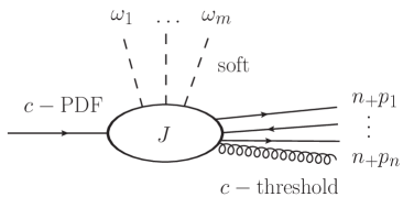
Figure 4: A pictorial, momentum-space, representation of a general matching equation.

4.2 Generalized soft functions

As we have seen in the previous section, explicit soft gauge fields from subleading-power Lagrangian terms play a passive role in the matching equation. The independent collinear functions are defined with respect to the independent soft structures. Hence, at subleading powers the explicit soft gauge fields are absorbed into the definition of soft functions, extending the LP result in (17), namely, we have

$$S_{i}(\Omega,\omega)=\int\frac{dx^{0}}{4\pi}e^{ix^{0}\Omega/2}\int\frac{dz_{-}}{2\pi}\,e^{-i\omega z_{-}}\frac{1}{N_{c}}\mbox{Tr}\langle 0|\mathbf{\bar{T}}\left[Y_{+}^{\dagger}(x^{0})Y_{-}(x^{0})\right]\mathbf{T}\left[Y_{-}^{\dagger}(0)Y_{+}(0){\mathfrak{s}_{i}(z_{-})}\right]|0\rangle.\quad\quad$$ (25)

These soft functions, unlike their LP counterparts, exhibit divergences at their lowest non-vanishing order. This leads to an interesting renormalization group structure and mixing with new soft functions [2, 4, 8, 21]. However, we do not explore their rich structure further here.

4.3 The factorization formula at NLP

Having discussed the new objects which appear in the schematic factorization formula beyond LP given in (18), we are in position to derive the precise form of factorization at NLP. We do not do this in detail here, as this derivation is rather technical and was carefully presented in Sec. 3 of [1]. We simply state that the NLP cross section is split into two contributions, the kinematic, where power corrections come from the expansion of phase space, and dynamical, which in turn are due to explicit insertions of subleading-power Lagrangian terms. We choose to define

$$\Delta(z)=\frac{1}{(1-\epsilon)}\frac{\hat{\sigma}(z)}{z}\,,$$ (26)

which makes the comparison with existing literature easier. The $\epsilon$ still appears as the factorization formula we derive is for $d$-dimensional regularized quantities.

One of the main results included in this contribution is the following all-order formulation of NLP factorization

$$\Delta^{dyn}_{{\rm{NLP}}}(z) = -\frac{2}{(1-\epsilon)}\,Q\left[\left(\frac{\not{n}_{-}}{4}\right){\gamma}_{\perp\rho}\left(\frac{\not{n}_{+}}{4}\right)\gamma^{\rho}_{\perp}\right]_{\beta\gamma}$$ (27)

$$\times\,\int d(n_{+}p)\,C^{\,{A0,A0}\,}(n_{+}p,x_{b}n_{-}{p}_{B})\,C^{*A0A0}\left(\,x_{a}n_{+}p_{A},\,x_{b}{n_{-}p_{B}}\right)$$

$$\times\,\sum^{5}_{i=1}\,\int\left\{d\omega_{j}\right\}{J}_{i,\gamma\beta}\left(n_{+}p,x_{a}n_{+}p_{A};\left\{\omega_{j}\right\}\right)\,{S}_{i}(\Omega;\left\{\omega_{j}\right\})+\rm{h.c.}\,,\quad$$

where here $\Omega=Q(1-z)$. The collinear functions are written in momentum space. We do not list all of the soft functions present in the above formula here, these can be found in Eqs. (3.34) - (3.39) of [1]. The spin trace present in LP result cannot yet be performed at this stage as there exist soft and collinear structures which share Dirac indices and must be contracted prior to performing the spin trace.

As pointed out above, the soft structures begin at the $\alpha_{s}$ order because of the explicit insertion of the soft fields. Interestingly, only one allowed soft structure contains exactly one soft gauge field. We will focus on this contribution in what follows. The soft function is given by

$${S}_{1}(\Omega;\omega) = \int\frac{dx^{0}}{4\pi}\,e^{i\Omega\,x^{0}/2}\int\frac{dz_{j-}}{2\pi}\,e^{-i\omega{z_{-}}}$$ (28)

$$\times\frac{1}{N_{c}}\,{\rm{Tr}}\langle 0|\bar{\mathbf{T}}\left[Y_{+}^{\dagger}(x^{0})Y_{-}(x^{0})\right]{\mathbf{T}}\left(\left[Y_{-}^{\dagger}(0)Y_{+}(0)\right]\frac{i\partial_{\perp}^{\nu}}{in_{-}\partial}\mathcal{B}^{+}_{\nu_{\perp}}\left(z_{-}\right)\right)|0\rangle\,,\quad$$

with the one-loop result (presented in expanded form in [2])

$$S^{(1)}_{1}\left(\Omega,\omega\right)=\frac{\alpha_{s}C_{F}}{2\pi}\frac{\mu^{2\epsilon}e^{\epsilon\gamma_{E}}}{\Gamma[1-\epsilon]}\,\frac{1}{\omega^{1+\epsilon}}\frac{1}{(\Omega-\omega)^{\epsilon}}\,\theta(\omega)\theta(\Omega-\omega)\,\,.\quad$$ (29)

This contribution is of interest to us, because the fact that it is the only soft structure which begins at $\mathcal{O}(\alpha_{s})$ means that the next-to-leading order (NLO) contribution is determined by it, and tree-level values for the hard function, $H(\hat{s})=|C^{A0,A0}(x_{a}n_{+}p_{A},x_{b}n_{-}p_{B})|^{2}$, and collinear function, $J_{1}$. Moreover, $J_{1}\otimes S_{1}$ is also the only contribution to the collinear sector at next-to-next-leading order (NNLO), as the rest of the soft functions begin already at $\mathcal{O}(\lambda^{2})$ and addition of a collinear loop yields N³LO terms. This is useful as we would like to study the new NLP collinear functions at one-loop order, and using this we can check the validity of our results to NNLO. We will discuss $J_{1}$ in more details in the next section.

We have neglected the kinematic corrections, $\Delta^{kin}$ since its structure is simpler than one of $\Delta^{dyn}$. However, it has been included in [1].

5 Collinear function at one-loop order and fixed-order check

The result for $J_{1}$ collinear function is another main result of this contribution and [1]. The calculation is a matching computation the operator equation in (23). It is rather involved and can be found in detail in Sec. 4 of [1]. Here we give the results and discuss the implications. The $J_{1}$ collinear function (with index structure restored for completeness) is given by

$${J}^{K(0)}_{1;\gamma\beta,fq}(n_{+}q,n_{+}p;\omega) = \mathbf{T}^{K}_{fq}\delta_{\beta\gamma}\left(-\frac{1}{n_{+}p}\delta(n_{+}q-n_{+}p)+2\,\frac{\partial}{\partial n_{+}q}\delta(n_{+}q-n_{+}p)\right),\qquad\,\,$$ (30)

at tree level, and

$${J}^{K\,(1)}_{1;\gamma\beta,fq}\left(n_{+}q,n_{+}p;\,\omega\right)=\frac{\alpha_{s}}{4\pi}\delta_{\gamma\beta}\mathbf{T}_{fq}^{K}\,\frac{1}{(n_{+}p)}\left(\frac{n_{+}p\,\omega}{\mu^{2}}\right)^{-\epsilon}\frac{e^{\epsilon\,\gamma_{E}}\,\Gamma[1+\epsilon]\Gamma[1-\epsilon]^{2}}{(-1+\epsilon)(1+\epsilon)\Gamma[2-2\epsilon]}$$

$$\hskip 42.67912pt\times\left(C_{F}\left(-\frac{4}{\epsilon}+3+8\epsilon+\epsilon^{2}\right)-C_{A}\left(-5+{8}{\epsilon}+\epsilon^{2}\right)\right)\delta(n_{+}q-n_{+}p)\qquad$$ (31)

$$\hskip 28.45274pt=\frac{\alpha_{s}}{4\pi}\,\frac{1}{(n_{+}p)}\,\delta_{\gamma\beta}\mathbf{T}_{fq}^{K}\bigg{(}C_{F}\left(\frac{4}{\epsilon}+5-4\ln\left(\frac{n_{+}p\,\omega}{\mu^{2}}\right)\right)-5\,C_{A}\bigg{)}\,\delta(n_{+}q-n_{+}p)+\,\mathcal{O}(\epsilon)\,,\qquad$$ (32)

at one-loop order. We have also expanded the result in $\epsilon$ for discussion. The NNLO collinear contribution is given by

$$\Delta^{dyn\,(2)}_{{\rm{NLP-coll}}}(z) = 4Q\,H^{(0)}\big{(}Q^{2}\big{)}\int d\omega\,{J}^{\,(1)}_{1}\left(x_{a}n_{+}p_{A};\omega\right)\,{S}^{\,(1)}_{1}(\Omega;\omega)\,,$$ (33)

where the delta function from the collinear function has been used already. Inserting $J_{1}$ from (5) and $S_{1}$ from (29) and performing the last integral gives

$$\Delta^{dyn\,(2)}_{{\rm{NLP-coll}}}(z) = \frac{\alpha_{s}^{2}}{(4\pi)^{2}}\Bigg{(}{C_{A}}C_{F}\left(\frac{20}{\epsilon}-(60\ln(1-z)-8)+\mathcal{O}(\epsilon)\right)$$

$$+C_{F}^{2}\,\bigg{(}-\frac{16}{\epsilon^{2}}+\frac{48\ln(1-z)-20}{\epsilon}+\left(-72\ln^{2}(1-z)+60\ln(1-z)+8\pi^{2}-24\right)+\mathcal{O}(\epsilon)\bigg{)}\,\Bigg{)}\,.$$

where we set $\mu=Q$. We note that leading logarithms, $\sim\alpha^{2}_{s}\ln^{3}(1-z)$ do not appear which is an indication that the definition used for collinear function is consistent [2]. The $C_{F}^{2}$ term in (5) is in agreement with the corresponding abelian contribution considered in Eq. (4.22) of [26] and Eqs. (13), (14) of [28] in the diagrammatic and expansion-by-regions methods respectively.

6 Ill-defined convolution

The last remark we wish to make, is with relation to the $\epsilon$ expanded result. To obtain Eq. (5) we have used $d$-dimensional quantities $J_{1}$ and $S_{1}$, performed the $\omega$ integral first and then expanded in $\epsilon$. If this order is reversed, that is, if we convolve renormalized objects, ill-defined terms such as $\int d\omega\,\delta(\omega)\,\ln(\omega)$ appear. This is an issue for extending NLP resummation beyond leading logarithmic order and is a open interesting conceptual challenge in the community, see for example [8]. With the results presented here we see the issue explicitly.

7 Summary

In this contribution we have outlined the formalism which can be used to describe general processes at subleading powers in $\lambda$ expansion. We have then used this formalism, focusing on the case of DY to motivate interesting structure of factorization at NLP, where new objects, the NLP collinear functions appear. We have also presented the new results for one-loop collinear function, using which the ill-defined convolution issue can be clearly seen. This contribution is meant as an overview of the formalism, with new interesting features mentioned but not derived step by step. A fuller, more detailed discussion is presented in [1].

References

- [1] M. Beneke, A. Broggio, S. Jaskiewicz and L. Vernazza, Threshold factorization of the Drell-Yan process at next-to-leading power, 1912.01585.
- [2] M. Beneke, A. Broggio, M. Garny, S. Jaskiewicz, R. Szafron, L. Vernazza et al., Leading-logarithmic threshold resummation of the Drell-Yan process at next-to-leading power, JHEP 03 (2019) 043, [1809.10631].
- [3] M. Beneke, F. Campanario, T. Mannel and B. D. Pecjak, Power corrections to decay spectra in the ‘shape-function’ region, JHEP 06 (2005) 071, [hep-ph/0411395].
- [4] M. Beneke, M. Garny, S. Jaskiewicz, R. Szafron, L. Vernazza and J. Wang, Leading-logarithmic threshold resummation of Higgs production in gluon fusion at next-to-leading power, 1910.12685.
- [5] M. Beneke, C. Bobeth and R. Szafron, Enhanced electromagnetic correction to the rare -meson decay , Phys. Rev. Lett. 120 (2018) 011801, [1708.09152].
- [6] M. Beneke, C. Bobeth and R. Szafron, Power-enhanced leading-logarithmic QED corrections to , JHEP 10 (2019) 232, [1908.07011].
- [7] S. Alte, M. Koenig and M. Neubert, Effective Field Theory after a New-Physics Discovery, JHEP 08 (2018) 095, [1806.01278].
- [8] I. Moult, I. W. Stewart, G. Vita and H. X. Zhu, The Soft Quark Sudakov, 1910.14038.
- [9] M. Beneke, A. P. Chapovsky, M. Diehl and T. Feldmann, Soft collinear effective theory and heavy to light currents beyond leading power, Nucl. Phys. B643 (2002) 431–476, [hep-ph/0206152].
- [10] M. Beneke and T. Feldmann, Multipole expanded soft collinear effective theory with non-abelian gauge symmetry, Phys. Lett. B553 (2003) 267–276, [hep-ph/0211358].
- [11] C. W. Bauer, S. Fleming, D. Pirjol and I. W. Stewart, An Effective field theory for collinear and soft gluons: Heavy to light decays, Phys. Rev. D63 (2001) 114020, [hep-ph/0011336].
- [12] C. W. Bauer, D. Pirjol and I. W. Stewart, Soft collinear factorization in effective field theory, Phys. Rev. D65 (2002) 054022, [hep-ph/0109045].
- [13] C. W. Bauer and I. W. Stewart, Invariant operators in collinear effective theory, Phys. Lett. B516 (2001) 134–142, [hep-ph/0107001].
- [14] M. Beneke, M. Garny, R. Szafron and J. Wang, Anomalous dimension of subleading-power N-jet operators, JHEP 03 (2018) 001, [1712.04416].
- [15] M. Beneke, M. Garny, R. Szafron and J. Wang, Anomalous dimension of subleading-power -jet operators. Part II, JHEP 11 (2018) 112, [1808.04742].
- [16] M. Beneke, M. Garny, R. Szafron and J. Wang, Violation of the Kluberg-Stern-Zuber theorem in SCET, JHEP 09 (2019) 101, [1907.05463].
- [17] I. Feige, D. W. Kolodrubetz, I. Moult and I. W. Stewart, A Complete Basis of Helicity Operators for Subleading Factorization, JHEP 11 (2017) 142, [1703.03411].
- [18] C.-H. Chang, I. W. Stewart and G. Vita, A Subleading Power Operator Basis for the Scalar Quark Current, JHEP 04 (2018) 041, [1712.04343].
- [19] M. A. Ebert, I. Moult, I. W. Stewart, F. J. Tackmann, G. Vita and H. X. Zhu, Power Corrections for N-Jettiness Subtractions at , JHEP 12 (2018) 084, [1807.10764].
- [20] I. Moult, I. W. Stewart and G. Vita, A subleading operator basis and matching for gg H, JHEP 07 (2017) 067, [1703.03408].
- [21] I. Moult, I. W. Stewart, G. Vita and H. X. Zhu, First Subleading Power Resummation for Event Shapes, JHEP 08 (2018) 013, [1804.04665].
- [22] T. Becher, M. Neubert and G. Xu, Dynamical Threshold Enhancement and Resummation in Drell- Yan Production, JHEP 07 (2008) 030, [0710.0680].
- [23] G. P. Korchemsky and G. Marchesini, Resummation of large infrared corrections using Wilson loops, Phys. Lett. B313 (1993) 433–440.
- [24] S. Moch and A. Vogt, Higher-order soft corrections to lepton pair and Higgs boson production, Phys. Lett. B631 (2005) 48–57, [hep-ph/0508265].
- [25] V. Del Duca, High-energy Bremsstrahlung Theorems for Soft Photons, Nucl. Phys. B345 (1990) 369–388.
- [26] D. Bonocore, E. Laenen, L. Magnea, S. Melville, L. Vernazza and C. D. White, A factorization approach to next-to-leading-power threshold logarithms, JHEP 06 (2015) 008, [1503.05156].
- [27] D. Bonocore, E. Laenen, L. Magnea, L. Vernazza and C. D. White, Non-abelian factorisation for next-to-leading-power threshold logarithms, JHEP 12 (2016) 121, [1610.06842].
- [28] D. Bonocore, E. Laenen, L. Magnea, L. Vernazza and C. D. White, The method of regions and next-to-soft corrections in Drell-Yan production, Phys. Lett. B742 (2015) 375–382, [1410.6406].