On the stability of Scott-Zhang type operators and application to multilevel preconditioning in fractional diffusion

Abstract

We provide an endpoint stability result for Scott-Zhang type operators in Besov spaces. For globally continuous piecewise polynomials these are bounded from $H^{3/2}$ into $B^{3/2}_{2,\infty}$; for elementwise polynomials these are bounded from $H^{1/2}$ into $B^{1/2}_{2,\infty}$. As an application, we obtain a multilevel decomposition based on Scott-Zhang operators on a hierarchy of meshes generated by newest vertex bisection with equivalent norms up to (but excluding) the endpoint case. A local multilevel diagonal preconditioner for the fractional Laplacian on locally refined meshes with optimal eigenvalue bounds is presented.

1 Introduction

The Scott-Zhang projection, originally introduced in [SZ90], is a very important tool in numerical analysis and has been generalized in various ways, [BG98, GS02, Car99, CH09, Ape99b, Aco01, Ran12, Cia13, FW15, AFF⁺15, KM15, EG17]. In its classical form, it is quasi-local, it is a projection onto the space of globally continuous, piecewise polynomials, it is stable in both $L^{2}$ and $H^{1}$ (and thus, by interpolation also in $H^{s}$, $s\in(0,1)$), and has optimal approximation properties. Therefore, it is well-suited for the analysis of classical finite element methods (FEMs), [BS02], and plays a key role in the analyses of, e.g., anisotropic finite elements, [Ape99a], adaptive finite element methods, [AFK⁺13], or mixed methods, [Bad12].

As globally continuous piecewise linear functions are not only in the Sobolev space $H^{1}(\Omega)$, but also in (fractional) Sobolev spaces $H^{3/2-\varepsilon}(\Omega)$ for any $\varepsilon>0$ — in fact, they are in the Besov space $B^{3/2}_{2,\infty}(\Omega)$ — a natural question is whether the operator is also stable in the stronger norms imposed on these spaces. In this article, we provide an endpoint stability result, i.e., study the stability in the norm $\|\cdot\|_{B^{3/2}_{2,\infty}}$, not only for the Scott-Zhang operator but more generally for local, $L^{2}(\Omega)$-stable operators with certain approximation properties in $L^{2}(\Omega)$ on shape-regular meshes. Additionally, we cover the case of operators such as the elementwise $L^{2}$-projection that map into spaces of discontinuous piecewise polynomials, where the corresponding endpoint space is $B^{1/2}_{2,\infty}$. By interpolation, these endpoint results imply stability results in the full range between $L^{2}$ and the Besov space.

Multilevel representations of Sobolev spaces (and Besov spaces) based on sequences of uniformly refined meshes are available in the literature; see, e.g., [Osw94, Sch98, BPV00], and the references there. Our stability for Scott-Zhang type operators allows us develop multilevel norm equivalences for spaces of globally continuous piecewise polynomials on adaptively refined meshes ${\mathcal{T}}$. These are assumed to be shape-regular and obtained by newest vertex bisection (NVB). The mesh hierarchy $\widetilde{{\mathcal{T}}}_{\ell}={\tt fcc}({\mathcal{T}},\widehat{{\mathcal{T}}}_{\ell})$, $\ell=0,\ldots,L$, is given by the finest common coarsening of ${\mathcal{T}}$ and the meshes $\widehat{{\mathcal{T}}}_{\ell}$ of a sequence $(\widehat{{\mathcal{T}}}_{\ell})_{\ell}$ of uniformly refined NVB-generated meshes. Our actual multilevel decomposition is then obtained with an adapted Scott-Zhang operator that is of independent interest (Lemma 4.4).

In numerics, an important application of multilevel decompositions is the design of multilevel additive Schwarz preconditioners, in particular multilevel diagonal scaling [DW91, Zha92] and BPX, [BPX91]. In this article, we propose a local multilevel diagonal preconditioner for the integral fractional Laplacian $(-\Delta)^{s}$ for $s\in(0,1)$ on adaptively refined meshes ${\mathcal{T}}_{\ell}$. The need for a preconditioner arises from the observation that the condition number of the stiffness matrix $\mathbf{A}^{\ell}\in{\mathbb{R}}^{N_{\ell}\times N_{\ell}}$ corresponding to a FEM discretization by piecewise linears of the integral fractional Laplacian grows like $\kappa(\mathbf{A}^{\ell})\sim N_{\ell}^{2s/d}\left(\frac{h^{\ell}_{\rm max}}{h^{\ell}_{\rm min}}\right)^{d-2s},$ where $h^{\ell}_{\rm max},h^{\ell}_{\rm min}$ denote the maximal and minimal mesh width of $\mathcal{T}_{\ell}$, see, e.g., [AMT99, AG17]. Since the fractional Laplacian on bounded domains features singularities at the boundary, typical meshes are strongly refined towards the boundary so that the quotient $h^{\ell}_{\rm max}/h^{\ell}_{\rm min}$ is large (see, e.g., [AG17, BBN⁺18, FMP19] for adaptively generated meshes). While the impact of the variation of the element size can be controlled by diagonal scaling (see, e.g., [AMT99]) the factor $N_{\ell}^{2s/d}$ persists. A good preconditioner is therefore required for an efficient iterative solution for large problem sizes $N_{\ell}$. Indeed, preconditioning for fractional differential operators has attracted attention recently. We mention multigrid preconditioners, [AG17] based on uniformly refined mesh hierarchies and operator preconditioning, [Hip06, GSUT19, SvV19], which requires one to realize an operator of the opposite order. Another, classical technique is the framework of additive Schwarz preconditioners, analyzed in a BPX-setting with Fourier techniques in [BLN19]. In the present work, we also adopt the additive Schwarz framework and show that, also in the presence of adaptively refined meshes, multilevel diagonal scaling leads to uniformly bounded condition numbers for the integral fractional Laplacian. The above mentioned norm equivalence of the multilevel decomposition provides the lower bound for the eigenvalues; an inverse estimate in fractional Sobolev norms, similarly to [FMP19], gives the upper bound for the eigenvalues. We mention that very closely related to preconditioning of discretizations of the fractional differential operators is earlier work on preconditioning for the hypersingular integral equation in boundary element methods (BEM), [TS96, TSM97, TSZ98, AM03, Mai09, FFPS17].

The present paper is structured as follows: Section 2 provides the necessary notation and states the three main results of the paper. The first result is the stability of quasi-interpolation operators in the endpoint Besov space (Theorem 2.2) both for globally continuous piecewise polynomials and discontinuous piecewise polynomials. The second result is a multilevel decomposition based on a modified Scott-Zhang operator on a mesh hierarchy of NVB meshes (Theorem 2.5). The third result is an optimal local multilevel diagonal preconditioner for the fractional Laplacian on adaptively generated meshes and the discretization by piecewise linears $S^{1,1}_{0}({\mathcal{T}})$ (for $s\in(0,1)$) and by piecewise constants $S^{0,0}({\mathcal{T}})$ (for $s\in(0,1/2)$). Two types of mesh hierarchies are considered: The first one is assumed to be generated by an adaptive algorithm and discussed in Theorem 2.6. The second one, $\widetilde{{\mathcal{T}}}_{\ell}={\tt fcc}({\mathcal{T}},\widehat{{\mathcal{T}}}_{\ell})$, is generated by taking the finest common coarsening of a fixed mesh ${\mathcal{T}}$ and a sequence of uniformly refined meshes $\widehat{{\mathcal{T}}}_{\ell}$; this is analyzed in Theorem 2.9.

Section 3 is concerned with the proof of the stability result of the quasi-interpolation operators in Besov spaces. Moreover, we present some extensions such as inverse estimates in Besov-norms (Lemma 3.6) or an interpolation result for discrete spaces in Besov-norms (Corollary 3.8).

In Section 4, we develop properties of the finest common coarsening of two meshes. We prove the norm equivalence for the multilevel decomposition. Furthermore, we develop, for given meshes ${\mathcal{T}}$, $\widehat{\mathcal{T}}$, two Scott-Zhang type operator $\widehat{I}^{SZ}$ and $\widetilde{I}^{SZ}$ on the meshes $\widehat{\mathcal{T}}$ and $\widetilde{{\mathcal{T}}}:={\tt fcc}({\mathcal{T}},\widehat{\mathcal{T}})$ with the property $\widehat{I}^{SZ}u=\widetilde{I}^{SZ}u$ for $u\in S^{p,1}({\mathcal{T}})$. Such operators are useful in various context and similar operators have been constructed, for example, in [DKS16, Lemma 3.5].

Finally, Section 5 provides the abstract analysis for the additive Schwarz method to prove the optimal bounds on the extremal eigenvalues of the preconditioned stiffness matrix for the fractional Laplacian on adaptively generated NVB meshes. Numerical experiments underline the optimality of the preconditioner.

Throughout the paper, we use the notation $\lesssim$ to abbreviate $\leq$ up to a generic constant $C>0$ that does not depend on critical parameters in our analysis. Moreover, we use $\simeq$ to indicate that both estimates $\lesssim$ and $\gtrsim$ hold.

2 Main results

2.1 Stability of (quasi-)interpolation operators in Besov spaces

Let $\Omega\subset{\mathbb{R}}^{d}$ be a bounded Lipschitz domain. For $s\geq 0$, we use the Sobolev spaces $H^{s}(\Omega)$, in the integer case $s\in{\mathbb{N}}_{0}$ defined in the standard way, see, e.g., [AF03], and for the fractional case $s\notin{\mathbb{N}}_{0}$ defined by interpolation, [Tar07]. We note that, equipped with the Aronstein-Slobodeckij (semi-)norm

$$\left\|u\right\|_{H^{s}(\Omega)}^{2}:=\left\|u\right\|_{L^{2}(\Omega)}^{2}+\left|u\right|_{H^{s}(\Omega)}^{2}\qquad\text{with}\quad\left|u\right|_{H^{s}(\Omega)}^{2}:=\int_{\Omega}\int_{\Omega}\frac{(u(x)-u(y))^{2}}{|x-y|^{d+2s}},$$

the space $H^{s}(\Omega)$ is a Hilbert space.

Moreover, for $s>0$, $s\notin{\mathbb{N}}_{0}$, $q\in[1,\infty]$, we employ the Besov spaces $B^{s}_{2,q}(\Omega)$ defined as the interpolation spaces $B^{s}_{2,q}(\Omega):=(H^{\sigma}(\Omega),H^{\sigma+1}(\Omega))_{\theta,q}$, where $\sigma=\lfloor s\rfloor$ and $\theta=s-\sigma\in(0,1)$. The norm is given by

$$\|u\|_{B_{2,q}^{s}(\Omega)}:=\begin{cases}\left(\int_{t=0}^{\infty}\left(t^{-\theta}K(t,u)\right)^{q}\frac{dt}{t}\right)^{1/q}&q\in[1,\infty),\\ \sup_{t>0}t^{-\theta}K(t,u)&q=\infty.\end{cases}$$

Here, for $u\in H^{\sigma}(\Omega)$ and $t>0$, the $K$-functional is defined by

$$K(t,u):=\inf_{u_{t}\in H^{\sigma+1}(\Omega)}\|u-u_{t}\|_{H^{\sigma}(\Omega)}+t\|u_{t}\|_{H^{\sigma+1}(\Omega)}.$$

For discretization, we assume that a regular (in the sense of Ciarlet) triangulation ${\mathcal{T}}$ of $\Omega$ consisting of open simplices is given. Additionally, ${\mathcal{T}}$ is assumed to be $\gamma$-shape regular in the sense

$$\max_{T\in{\mathcal{T}}}(\operatorname*{diam}(T)/\left|T\right|^{1/d})\leq\gamma<\infty,$$

where $\operatorname*{diam}(T):=\sup_{x,y\in T}\left|x-y\right|$ and $\left|T\right|$ is the volume of $T$. By $h\in L^{\infty}(\Omega)$, we denote the piecewise constant mesh size function satisfying $h|_{T}:=h_{T}:=\left|T\right|^{1/d}$ for $T\in{\mathcal{T}}$.

Let $P_{p}(T)$ be the space of polynomials of (maximal) degree $p$ on the element $T\in{\mathcal{T}}$. Then, the spaces of ${\mathcal{T}}$-piecewise polynomials of degree $p\in{\mathbb{N}}_{0}$ and regularity $m\in{\mathbb{N}}_{0}$ are defined by

$$S^{p,m}(\mathcal{T}) :=\left\{u\in H^{m}(\Omega)\colon u|_{T}\in P_{p}(T)\quad\forall T\in\mathcal{T}\right\},$$

$$S^{p,m}_{0}(\mathcal{T}) :=S^{p,m}(\mathcal{T})\cap H^{1}_{0}(\Omega)\qquad m\geq 0.$$

For $T\in\mathcal{T}$ the element patch

$$\omega(T):=\omega^{1}(T):=\operatorname*{interior}\left(\bigcup\{\overline{T^{\prime}}\colon T^{\prime}\in{\mathcal{T}},\overline{T^{\prime}}\cap\overline{T}\neq\emptyset\}\right),$$

consists of the element $T$ and all its neighbors. Inductively, the $k$-th order patch is defined by

$$\omega^{k}(T):=\operatorname*{interior}\left(\bigcup\{\overline{T^{\prime}}\colon T^{\prime}\in{\mathcal{T}},\overline{T^{\prime}}\cap\overline{\omega^{k-1}(T)}\neq\emptyset\}\right).$$

In the following, we study (quasi-)interpolation operators $I_{h}^{m}$ satisfying the following locality, stability and approximation properties.

Assumption 2.1.

Let $m\geq 1$ and $I_{h}^{m}$ be an operator $I_{h}^{m}:L^{2}(\Omega)\rightarrow S^{p,m-1}({\mathcal{T}})$ that satisfies:

1. Quasi-locality: For every $T\in{\mathcal{T}}$ the restriction $(I_{h}^{m}u)|_{T}$ depends solely on $u|_{\omega(T)}$.

2. Stability in $L^{2}$: For $u\in L^{2}(\Omega)$, there holds

   $$\|I_{h}^{m}u\|_{L^{2}(T)}\leq C\|u\|_{L^{2}(\omega(T))}.$$

3. Approximation properties of $m$-th order: For $u\in H^{m}(\Omega)$, there holds

   $$\|u-I_{h}^{m}u\|_{L^{2}(T)}\leq Ch_{T}^{m}\|u\|_{H^{m}(\omega(T))}.$$

The constants in (ii) and (iii) depend only on $\Omega$, $d$, $m$, $p$, and the $\gamma$-shape regularity of ${\mathcal{T}}$.

The following theorem is the main result of this subsection and states a stability result in the Besov space $B^{m-1/2}_{2,\infty}(\Omega)$ for operators satisfying Assumption 2.1. Its proof will be given in Section 3.1 below.

Theorem 2.2.

Fix $m\in\{1,2\}$ and $p\in{\mathbb{N}}_{0}$ with $p\geq m-1$. Let an operator $I_{h}^{m}$ satisfying Assumption 2.1 be given. Then, for all $u\in H^{m-1/2}(\Omega)$, we have

$$\|I_{h}^{m}u\|_{B^{m-1/2}_{2,\infty}(\Omega)}\leq C\|u\|_{H^{m-1/2}(\Omega)},$$ (2.1)

where the constant $C>0$ depends solely on $\Omega$, $d$, $m$ ,$p$, and the $\gamma$-shape regularity of ${\mathcal{T}}$.

If the mesh ${\mathcal{T}}$ is additionally quasi-uniform, then, for all $u\in B^{m-1/2}_{2,\infty}(\Omega)$, the sharper estimate

$$\|I_{h}^{m}u\|_{B^{m-1/2}_{2,\infty}(\Omega)}\leq C\|u\|_{B^{m-1/2}_{2,\infty}(\Omega)}$$ (2.2)

holds.

Remark 2.3.

For $m=1$, a possible choice for $I_{h}^{m}$ is the $L^{2}(\Omega)$-orthogonal projection that trivially satisfies Assumption 2.1. For $m=2$ the Scott-Zhang projection, introduced in [SZ90] and defined below, is an example of an operator $I_{h}^{m}$ satisfying Assumption 2.1. Therefore, Theorem 2.2 provides a novel stability estimates for these projection operators in Besov spaces.  

2.2 Multilevel decomposition based on mesh hierarchies generated by NVB

The multilevel decompositions will be based on mesh hierarchies that are engendered by newest vertex bisection (NVB). For discussion of properties of NVB meshes we refer to [KPP13] for the case $d=2$ and to [Ste08] for the case $d\geq 3$. We consider sequences of regular meshes that are obtained by NVB-refinement from an initial mesh ${\mathcal{T}}_{0}$.

2.2.1 The finest common coarsening

For two regular triangulations ${\mathcal{T}}$, ${\mathcal{T}}^{\prime}$ (obtained by NVB from the same triangulation $\widehat{\mathcal{T}}_{0}$), we define the finest common coarsening as

$${\tt fcc}({\mathcal{T}},{\mathcal{T}}^{\prime}):=$$ (2.3)

$$\qquad\underbrace{\{T\in{\mathcal{T}}\,:\,\exists T^{\prime}\in{\mathcal{T}}^{\prime}\mbox{ s.t. }T^{\prime}\subsetneq T\}}_{=:\mathfrak{T}_{1}}\cup\underbrace{\{T^{\prime}\in{\mathcal{T}}^{\prime}\,:\,\exists T\in{\mathcal{T}}\mbox{ s.t. }T\subsetneq T^{\prime}\}}_{=:\mathfrak{T}_{2}}\cup\underbrace{({\mathcal{T}}\cap{\mathcal{T}}^{\prime})}_{=:\mathfrak{T}_{3}}.$$

We refer to Lemma 4.1 for the proofs that the three sets in the definition of the finest common coarsening are pairwise disjoint and that ${\tt fcc}({\mathcal{T}},{\mathcal{T}}^{\prime})$ is indeed a regular triangulation of $\Omega$.

Let $\widehat{\mathcal{T}}_{\ell}$ be the uniform refinement of $\widehat{\mathcal{T}}_{0}$ of level $\ell$. We call $\operatorname*{level}(T):=\ell$ the level of an element $T\in\widehat{\mathcal{T}}_{\ell}$. Given a regular triangulation ${\mathcal{T}}$, we will consider

$$\widetilde{\mathcal{T}}_{\ell}:={\tt fcc}({\mathcal{T}},\widehat{\mathcal{T}}_{\ell}),$$

which is in general a coarser mesh than the uniform triangulation $\widehat{\mathcal{T}}_{\ell}$.

2.2.2 Adapted Scott-Zhang operators

We recall the basic construction of the Scott-Zhang operator of [SZ90] or [BS02, Sec. 4.8]. It will be convenient in the proof of Lemma 4.4 to use Lagrange bases of the space $S^{p,1}({\mathcal{T}}^{\prime})$ defined on a mesh ${\mathcal{T}}^{\prime}$, where ${\mathcal{T}}^{\prime}$ is either $\widehat{\mathcal{T}}_{\ell}$ or ${\tt fcc}({\mathcal{T}},\widehat{\mathcal{T}}_{\ell})$.

1. On the reference $d$-simplex $\widehat{T}=\operatorname*{conv}\{z_{1},\dots,z_{d+1}\}$, let the $\operatorname{dim}P_{p}$ nodes ${\mathcal{N}}(\widehat{T})$ be the regularly spaced nodes as described in [Cia78, Sec. 2.2] (called “principal lattice” there),

   $$\mathcal{N}(\widehat{T}):=\Big{\{}x=\sum_{j=1}^{d+1}\lambda_{j}z_{j}\,:\,\sum_{j=1}^{d+1}\lambda_{j}=1,\;\lambda_{j}\in\Big{\{}\frac{i}{p},i=0,\dots,p\Big{\}}\Big{\}}.$$

   We note that any polynomial in $P_{p}$ is uniquely determined by its values on $\mathcal{N}(\widehat{T})$.

2. The nodes ${\mathcal{N}}({\mathcal{T}}^{\prime})\subset\overline{\Omega}$ for the mesh ${\mathcal{T}}^{\prime}$ are the push-forward of the nodes of ${\mathcal{N}}(\widehat{T})$ under the element maps. The Lagrange basis $\{\varphi_{z,{\mathcal{T}}^{\prime}}\,|\,z\in{\mathcal{N}}({\mathcal{T}}^{\prime})\}$ of $S^{p,1}({\mathcal{T}}^{\prime})$ (with respect to the nodes ${\mathcal{N}}({\mathcal{T}}^{\prime})$) is characterized by $\varphi_{z,{\mathcal{T}}^{\prime}}(z^{\prime})=\delta_{z,z^{\prime}}$ for all $z$, $z^{\prime}\in{\mathcal{N}}({\mathcal{T}}^{\prime})$; here, $\delta_{z,z^{\prime}}$ is the Kronecker Delta defined as $\delta_{z,z^{\prime}}=1$ if $z=z^{\prime}$ and $\delta_{z,z^{\prime}}=0$ for $z\neq z^{\prime}$.

3. The basis functions $\varphi_{z,{\mathcal{T}}^{\prime}}$ have the following support properties: a) if $z\in T$ for some $T\in{\mathcal{T}}^{\prime}$, then $\operatorname{supp}\varphi_{z,{\mathcal{T}}^{\prime}}\subset\overline{T}$; b) if $z\in f$ for some $j$-dimensional face ($j<d$) of $T$, then $\operatorname{supp}\varphi_{z,{\mathcal{T}}^{\prime}}\subset\omega_{f}$, where $\omega_{f}=\operatorname{int}\bigcup\{\overline{T}\colon f\mbox{ is $j$-face of $T\in{\mathcal{T}}^{\prime}$}\}$. In particular, if $z\not\in\overline{T}$, then $\operatorname{supp}\varphi_{z,{\mathcal{T}}^{\prime}}\cap T=\emptyset$.

4. For each element $T\in{\mathcal{T}}^{\prime}$, one has a dual basis $\{\varphi^{\ast}_{z,T}\,:\,z\in\overline{T}\}\subset P_{p}(T)$ of $P_{p}(T)$, i.e., $\int_{T}\varphi^{\ast}_{z,T}\varphi_{z^{\prime},{\mathcal{T}}^{\prime}}=\delta_{z,z^{\prime}}$ for all nodes $z$, $z^{\prime}\in\overline{T}$. In particular, this gives

   $$\int_{T}\varphi^{\ast}_{z,T}u\,dx=u(z)\qquad\forall T\in{\mathcal{T}}^{\prime}\quad\forall u\in P_{p}(T).$$ (2.4)

5. For each node $z\in{\mathcal{N}}({\mathcal{T}}^{\prime})$, define the admissible set of averaging elements as ${\mathcal{A}}(z,{\mathcal{T}}^{\prime}):=\{T\in{\mathcal{T}}^{\prime}\colon z\in\overline{T}\}$. A Scott-Zhang operator is then defined by selecting, for each $z$, a $T_{z}\in{\mathcal{A}}(z,{\mathcal{T}}^{\prime})$ and setting

   $$I^{SZ}u:=\sum_{z\in{\mathcal{N}}({\mathcal{T}}^{\prime})}\varphi_{z,{\mathcal{T}}^{\prime}}\left(\int_{T_{z}}\varphi^{\ast}_{z,T_{z}}u\,dx\right).$$ (2.5)

For nodes $z$ that are on the boundary of an element, the admissible set ${\mathcal{A}}(z,{\mathcal{T}}^{\prime})$ has more than one element. However, from (2.4), we get that the values of the functionals coincide on $S^{p,1}({\mathcal{T}}^{\prime})$:

$$\int_{T_{z}}\varphi^{\ast}_{z,T_{z}}u\;dx=u(z)=\int_{T^{\prime}_{z}}\varphi^{\ast}_{z,T^{\prime}_{z}}\,u\,dx\qquad\forall T_{z},T^{\prime}_{z}\in{\mathcal{A}}(z,{\mathcal{T}})\quad\forall u\in S^{p,1}({\mathcal{T}}^{\prime}).$$ (2.6)

We also highlight that (2.4) implies that $I^{SZ}$ is a projection onto $S^{p,1}({\mathcal{T}})$. Such Scott-Zhang operators satisfy the stability and approximation properties of Assumption 2.1 with constants that solely depend on $p$, the specific choice polynomial basis, the shape-regularity of the underlying triangulation, and $\Omega$. In particular, the constants are independent of the specific choice of averaging region $T_{z}$.

The freedom in the choice of the averaging element $T_{z}$ can be exploited to ensure additional properties, see also [DKS16, Sec. 3],[FFPS17, Sec. 4.3]. A guiding principle in the following definition of our modified Scott-Zhang operator is that in the definition of $\widetilde{I}^{SZ}$ one selects the averaging element $T_{z}$ from the mesh ${\mathcal{T}}$ whenever possible:

Definition 2.4 (adapted Scott-Zhang operators).

For given ${\mathcal{T}}$ that is obtained by NVB-refinement from a regular triangulation $\widehat{\mathcal{T}}_{0}$ and $\widetilde{\mathcal{T}}_{\ell}={\tt fcc}({\mathcal{T}},\widehat{\mathcal{T}}_{\ell})$, the operators $\widetilde{I}^{SZ}_{\ell}:L^{2}(\Omega)\rightarrow\widetilde{V}_{\ell}=S^{p,1}(\widetilde{\mathcal{T}}_{\ell})$ and $\widehat{I}^{SZ}_{\ell}:L^{2}(\Omega)\rightarrow\widehat{V}_{\ell}=S^{p,1}(\widehat{\mathcal{T}}_{\ell})$ are Scott-Zhang operators as defined in (2.5) with the following choice of averaging element $T_{z}$ for $\widetilde{I}^{SZ}_{\ell}$ and $\widehat{I}^{SZ}_{\ell}$:

1. First, loop through all $T\in\widehat{\mathcal{T}}_{\ell}\cap\widetilde{\mathcal{T}}_{\ell}$ (in any fixed order) and select the averaging sets $T_{z}$ for the nodes $z\in\overline{T}$ as follows:

   1. If $z\in T$, then select $T_{z}=T$ for both $\widehat{I}^{SZ}_{\ell}$ and $\widetilde{I}^{SZ}_{\ell}$.

   2. If $z\in\partial T$ and the node $z$ has not been assigned an averaging set $T_{z}$ yet, then:

      1. If ${\mathcal{A}}(z,\widehat{\mathcal{T}}_{\ell})$ contains an element $T^{\prime}\in\widehat{\mathcal{T}}_{\ell}$ that is a proper subset of an element $\widetilde{T}\in{\mathcal{T}}$, then select this $T^{\prime}$ to define $\widehat{I}^{SZ}_{\ell}$ and select $\widetilde{T}$ for the definition of $\widetilde{I}^{SZ}_{\ell}$.

      2. Else select $T$ for both $\widehat{I}^{SZ}_{\ell}$ and $\widetilde{I}^{SZ}_{\ell}$.

2. Next, loop through all $T\in\widetilde{\mathcal{T}}_{\ell}\setminus\widehat{\mathcal{T}}_{\ell}$ (in any fixed order). Select, for the construction of $\widetilde{I}^{SZ}_{\ell}$, this $T$ as the averaging element for all nodes $z$ with $z\in\overline{T}$ that have not already been fixed in step (1) or in a previous step of the loop. This completes the definition of $\widetilde{I}^{SZ}_{\ell}$.

3. Finally, loop through all $T\in\widehat{\mathcal{T}}_{\ell}\setminus\widetilde{\mathcal{T}}_{\ell}$ (in any fixed order). Select, for the construction of $\widehat{I}^{SZ}_{\ell}$, this $T$ as the averaging element for all nodes $z$ with $z\in\overline{T}$ that have not already been fixed in step (1) or in a previous step of the loop. This completes the definition of $\widehat{I}^{SZ}_{\ell}$.

We note, that this definition of the adapted Scott-Zhang operators is exploited to show $\widehat{I}^{SZ}_{\ell}u=\widetilde{I}^{SZ}_{\ell}u$ for all $u\in S^{p,1}({\mathcal{T}})$, which is proven in Lemma 4.4 below.

2.2.3 The multilevel decomposition

With the use of the adapted Scott-Zhang operators $\widetilde{I}^{SZ}_{\ell}$ and a mesh hierarchy based on NVB meshes and the finest common coarsening between theses meshes and uniform refined meshes, we obtain a multilevel decomposition with norm equivalence in the Besov space $B^{3\theta/2}_{2,q}(\Omega)$ as a consequence of the stability estimate of Theorem 2.2.

Theorem 2.5.

Let ${\mathcal{T}}$ be a mesh obtained by NVB-refinement of a triangulation $\widehat{\mathcal{T}}_{0}$ with mesh size $\widehat{h}_{0}$. Let $\widehat{\mathcal{T}}_{\ell}$ be the sequence of uniformly refined meshes starting from $\widehat{\mathcal{T}}_{0}$ with mesh size $\widehat{h}_{\ell}=\widehat{h}_{0}2^{-\ell}$. Set $\widetilde{\mathcal{T}}_{\ell}:={\tt fcc}({\mathcal{T}},\widehat{\mathcal{T}}_{\ell})$. Let $\widetilde{I}^{SZ}_{\ell}:L^{2}(\Omega)\rightarrow S^{p,1}(\widetilde{\mathcal{T}}_{\ell})$ be the adapted Scott-Zhang operator defined in Definition 2.4. Then, on the space $S^{p,1}({\mathcal{T}})$ the following three norms are equivalent with equivalence constants depending only on $\widehat{\mathcal{T}}_{0}$, $p$, $\theta\in(0,1)$, and $q\in[1,\infty]$:

$$\|u\|_{B^{3\theta/2}_{2,q}(\Omega)},$$

$$\|\widetilde{I}^{SZ}_{0}u\|_{L^{2}(\Omega)}+\|(2^{3\theta\ell/2}\|u-\widetilde{I}^{SZ}_{\ell}u\|_{L^{2}(\Omega)})_{\ell\geq 0}\|_{\ell^{q}},$$

$$\|\widetilde{I}^{SZ}_{0}u\|_{L^{2}(\Omega)}+\|(2^{3\theta\ell/2}\|Q_{\ell}u\|_{L^{2}(\Omega)})_{\ell\geq 0}\|_{\ell^{q}},$$

where $Q_{\ell}=\widetilde{I}^{SZ}_{\ell+1}-\widetilde{I}^{SZ}_{\ell}$.

2.3 A realization of an optimal multilevel preconditioner for the fractional Laplacian

The final main result of this paper presents a multilevel diagonal preconditioner with uniformly bounded condition number on locally refined triangulations for the fractional Laplacian.

With the integral fractional Laplacian defined as the principal value integral

$$(-\Delta)^{s}u(x):=C(d,s)\,\text{P.V.}\int_{\mathbb{R}^{d}}\frac{u(x)-u(y)}{|x-y|^{d+2s}}dy\qquad C(d,s):=2^{2s}s\frac{\Gamma(s+d/2)}{\pi^{d/2}\Gamma(1-s)},$$

where $\Gamma(\,\cdot\,)$ denotes the Gamma function, we consider the equation

$$(-\Delta)^{s}u =f\qquad\text{in}\quad\Omega,$$

$$u =0\qquad\text{in}\quad\Omega^{c}$$ (2.7)

for a given right-hand side $f\in H^{-s}(\Omega)$. Here, $H^{-s}(\Omega)$ denotes the dual space of the Hilbert space

$$\widetilde{H}^{s}(\Omega)=\{u\in H^{s}(\mathbb{R}^{d})\,:\,u\equiv 0\,\,\text{on}\,\,\Omega^{c}\},\qquad\left\|v\right\|_{\widetilde{H}^{s}(\Omega)}^{2}:=\left\|v\right\|_{H^{s}(\Omega)}^{2}+\left\|v/\rho^{s}\right\|_{L^{2}(\Omega)}^{2},$$

where $\rho(x)=\operatorname{dist}(x,\partial\Omega)$ is the distance of a point $x\in\Omega$ to the boundary $\partial\Omega$.

The weak formulation of (2.3) is given by finding $u\in\widetilde{H}^{s}(\Omega)$ such that

$$a(u,v):=\frac{C(d,s)}{2}\int\int_{{\mathbb{R}}^{d}\times{\mathbb{R}}^{d}}\frac{(u(x)-u(y))(v(x)-v(y))}{\left|x-y\right|^{d+2s}}\,dx\,dy=\int_{\Omega}fv\,dx\quad\forall v\in\widetilde{H}^{s}(\Omega).$$ (2.8)

Existence and uniqueness of $u\in\widetilde{H}^{s}(\Omega)$ follow from the Lax–Milgram lemma.

With a given regular triangulation ${\mathcal{T}}_{0}$, we consider two hierarchical sequence of meshes $\mathcal{T}_{\ell}$, $\widetilde{\mathcal{T}}_{\ell}$, $\ell=0,\dots,L$:

1. $\mathcal{T}_{\ell}$ is generated by an adaptive algorithm (see, e.g., [Dör96]) of the form SOLVE – ESTIMATE – MARK – REFINE, where the step REFINE is done by newest vertex bisection. In the following, both for the case of piecewise linear and piecewise constant basis function, we always assume that the meshes ${\mathcal{T}}_{\ell}$ are regular in the sense of Ciarlet.

2. From a given triangulation ${\mathcal{T}}_{L}$ obtained by NVB refinement of ${\mathcal{T}}_{0}$ - e.g. given from an adaptive algorithm - the finest common coarsening with the uniform refinements of ${\mathcal{T}}_{0}$, denoted by $\widehat{\mathcal{T}}_{\ell}$, provides a hierarchy of meshes $\widetilde{\mathcal{T}}_{\ell}={\tt fcc}(\mathcal{T}_{L},\widehat{\mathcal{T}}_{\ell})$.

2.3.1 A local multilevel diagonal preconditioner for adaptively refined meshes

We start with the case of the adaptively generated mesh hierarchy $({\mathcal{T}}_{\ell})_{\ell}$. On the mesh ${\mathcal{T}}_{\ell}$ we discretize with piecewise constants (for $0<s<1/2$) in the space $V_{\ell}^{0}=S^{0,0}(\mathcal{T}_{\ell})$ and piecewise linears (for $0<s<1$) in the space $V_{\ell}^{1}=S^{1,1}_{0}(\mathcal{T}_{\ell})$. If the distinction between $V_{\ell}^{0}$ and $V_{\ell}^{1}$ is not essential, we write $V_{\ell}$ meaning $V_{\ell}\in\{V_{\ell}^{0},V_{\ell}^{1}\}$. The Galerkin discretization (2.3) in $V_{\ell}$ of reads as: Find $u_{\ell}\in V_{\ell}$, such that

$$a(u_{\ell},v_{\ell})=\left<f,v_{\ell}\right>_{L^{2}(\Omega)}\qquad\forall v_{\ell}\in V_{\ell}.$$ (2.9)

Moreover, on the uniform refined meshes $\widehat{\mathcal{T}}_{\ell}$, in the same way, we define the discrete spaces

$$\widehat{V}_{\ell}^{0}=S^{0,0}(\mathcal{T}_{\ell}),\quad\widehat{V}_{\ell}^{1}=S^{1,1}_{0}(\mathcal{T}_{\ell}),\qquad\text{and}\quad\widehat{V}_{\ell}\in\{\widehat{V}_{\ell}^{0},\widehat{V}_{\ell}^{1}\}.$$

We define sets of “characteristic” points $\mathcal{N}_{\ell}^{i}$, $i=0,1$ representing the degrees of freedom of $V_{\ell}$. For the piecewise constant case $V_{\ell}^{0}$, the set $\mathcal{N}_{\ell}^{0}$ contains all barycenters of elements of the mesh ${\mathcal{T}}_{\ell}$. For the piecewise linear case $V_{\ell}^{1}$, we denote the set of all interior vertices of the mesh $\mathcal{T}_{\ell}$ by $\mathcal{N}_{\ell}^{1}$. If the distinction between $\mathcal{N}_{\ell}^{0}$ and $\mathcal{N}_{\ell}^{1}$ is not essential, we will write $\mathcal{N}_{\ell}$ meaning $\mathcal{N}_{\ell}\in\{\mathcal{N}_{\ell}^{0},\mathcal{N}_{\ell}^{1}\}$ is either $\mathcal{N}_{\ell}^{0}$ if $V_{\ell}=V_{\ell}^{0}$ or $\mathcal{N}_{\ell}^{1}$ if $V_{\ell}=V_{\ell}^{1}$ and call $z\in\mathcal{N}_{\ell}$ nodes.

We choose a basis of $V_{\ell}=\operatorname*{span}\{\varphi^{\ell}_{z_{j}},z_{j}\in\mathcal{N}_{\ell},j=1,\dots,N_{\ell}\}$ – for the piecewise constants we take the characteristic functions $\varphi_{z_{j}}^{\ell}=\chi_{T_{j}}$ of the element satisfying $z_{j}\in T_{j}\in\mathcal{T}_{\ell}$, and for the piecewise linears we take hat functions corresponding to the interior nodes defined by $\varphi_{z_{j}}^{\ell}(z_{i})=\delta_{j,i}$ for all nodes $z_{i}\in\mathcal{N}_{\ell}$. With these bases, we can write $u_{\ell}=\sum_{j=1}^{N_{\ell}}\mathbf{x}^{\ell}_{j}\varphi_{z_{j}}^{\ell}$, and (2.9) is equivalent to solving the linear system

$$\mathbf{A}^{\ell}\mathbf{x}^{\ell}=\mathbf{b}^{\ell}$$ (2.10)

with the stiffness matrix $\mathbf{A}^{\ell}$ and load vector $\mathbf{b}^{\ell}$

$$\mathbf{A}^{\ell}_{kj}:=a(\varphi_{z_{j}}^{\ell},\varphi_{z_{k}}^{\ell}),\qquad\mathbf{b}_{k}^{\ell}:=\left<f,\varphi_{z_{k}}^{\ell}\right>_{L^{2}(\Omega)}.$$ (2.11)

Again, we mention that the condition number of the unpreconditioned Galerkin matrix grows like $\kappa(\mathbf{A}^{\ell})\sim N_{\ell}^{2s/d}\left(\frac{h^{\ell}_{\rm max}}{h^{\ell}_{\rm min}}\right)^{d-2s},$ which stresses the need for a preconditioner in order to use an iterative solver.

For fixed $L\in{\mathbb{N}}_{0}$, we introduce a local multilevel diagonal preconditioner $(\mathbf{B}^{L})^{-1}$ of BPX-type for the stiffness matrix $\mathbf{A}^{L}$ from (2.10) in the same way as in [FFPS17, AM03]. That is, following [FFPS17], we define the patch of a node $z\in\mathcal{N}_{\ell}$ as

$$\omega_{\ell}(z):=\operatorname*{interior}\bigcup\{\overline{T}\,:\,T\in{\mathcal{T}}_{\ell},z\in\overline{T}\}.$$

The sets $\mathcal{M}_{\ell}^{i}$, $i=0,1$, defined in the following describe the changes in the mesh hierarchy between the level $\ell$ and $\ell-1$ and are crucial for the definition of the local diagonal scaling. For the case of piecewise linears, we define the sets $\mathcal{M}_{\ell}^{1}$ as the sets of new vertices and their direct neighbors in the mesh ${\mathcal{T}}_{\ell}$: We set $\mathcal{M}_{0}^{1}:=\mathcal{N}_{0}^{1}$ and

$$\mathcal{M}_{\ell}^{1}:=\mathcal{N}_{\ell}^{1}\backslash\mathcal{N}_{\ell-1}^{1}\cup\{z\in\mathcal{N}_{\ell}^{1}\cap\mathcal{N}_{\ell-1}^{1}\,:\,\omega_{\ell}(z)\subsetneqq\omega_{\ell-1}(z)\}\quad\ell\geq 1.$$ (2.12)

For the case of a piecewise constant discretization, we define the set $\mathcal{M}_{\ell}^{0}$ simply as the barycenters corresponding to the new elements, i.e., $\mathcal{M}_{\ell}^{0}:=\mathcal{N}_{\ell}^{0}\backslash\mathcal{N}_{\ell-1}^{0}$ for $\ell\geq 1$. In the same way as for the nodes $\mathcal{N}_{\ell}$ we write $\mathcal{M}_{\ell}$ to either be $\mathcal{M}_{\ell}^{0}$ and $\mathcal{M}_{\ell}^{1}$, which should be clear from context.

The local multilevel diagonal preconditioner is given by

$$(\mathbf{B}^{L})^{-1}:=\sum_{\ell=0}^{L}\mathbf{I}^{\ell}\;\mathbf{D}^{\ell}_{\rm inv}(\mathbf{I}^{\ell})^{T},$$ (2.13)

where, with $N_{\ell}:=\#\mathcal{N}_{\ell}$, the appearing matrices are defined as

• $\mathbf{I}^{\ell}\in\mathbb{R}^{N_{L}\times N_{\ell}}$ denotes the identity matrix corresponds to the embedding $\mathcal{I}^{\ell}:V_{\ell}\rightarrow V_{L}$.

• $\mathbf{D}^{\ell}_{\rm inv}\in\mathbb{R}^{N_{\ell}\times N_{\ell}}$ is a diagonal matrix with entries $(\mathbf{D}^{\ell}_{\rm inv})_{jk}=\begin{cases}(\mathbf{A}^{\ell}_{jj})^{-1}\delta_{jk}&j\;:\;z_{j}\in\mathcal{M}_{\ell},\\ 0&\text{ otherwise}\end{cases},$ i.e., the entries of the diagonal matrix are the inverse diagonal entries of the matrix $\mathbf{A}^{\ell}$ corresponding to the degrees of freedom in $\mathcal{M}_{\ell}$.

Moreover, we define the additive Schwarz matrix $\mathbf{P}_{AS}^{L}:={(\mathbf{B}^{L})}^{-1}\mathbf{A}^{L}$. Instead of solving (2.10) for $\ell=L$, we solve the following preconditioned linear systems

$$\mathbf{P}_{AS}^{L}\mathbf{x}^{L}={(\mathbf{B}^{L})}^{-1}\mathbf{b}^{L}.$$ (2.14)

The following theorem is the main result of this section and provides the optimal bounds to the eigenvalues of the preconditioned matrix.

Theorem 2.6.

The minimal and maximal eigenvalues of the additive Schwarz matrix $\mathbf{P}_{AS}^{L}$ are bounded by

$$c\leq\lambda_{\min}\left(\mathbf{P}_{AS}^{L}\right)\qquad\text{and}\qquad\lambda_{\max}\left(\mathbf{P}_{AS}^{L}\right)\leq C,$$ (2.15)

where the constants $c$, $C>0$ depend only on $\Omega$, $d$, $s$, and the initial triangulation ${\mathcal{T}}_{0}$.

Remark 2.7.

The preconditioner $(\mathbf{B}^{L})^{-1}$ is a symmetric positive definite matrix and the preconditioned matrix $\mathbf{P}_{AS}^{L}$ is symmetric and positive definite with respect to the inner-product induced by $\mathbf{B}^{L}$. Therefore, Theorem 2.6 leads to $\kappa(\mathbf{P}_{AS}^{L})\leq C/c$.  

Remark 2.8.

The cost to apply the preconditioner is proportional to $\sum_{\ell=0}^{L}\operatorname{card}\mathcal{M}_{\ell}=O(N_{L})$ by [FFPS17, Sec. 3.1].  

2.3.2 A local multilevel diagonal preconditioner using a finest common coarsening mesh hierarchy

In this subsection, we provide a result similar to Theorem 2.6 for the meshes $\widetilde{\mathcal{T}}_{\ell}={\tt fcc}(\mathcal{T}_{L},\widehat{\mathcal{T}}_{\ell})$, where $\ell=0,\dots,L$.

With $\widetilde{V}_{\ell}^{0}=S^{0,0}(\widetilde{{\mathcal{T}}}_{\ell})$, $\widetilde{V}_{\ell}^{1}=S^{1,1}_{0}(\widetilde{{\mathcal{T}}}_{\ell})$, and $\widetilde{V}_{\ell}\in\{\widetilde{V}_{\ell}^{0},\widetilde{V}_{\ell}^{1}\}$ being either the piecewise constants or piecewise linears on $\widetilde{\mathcal{T}}_{\ell}$, the Galerkin discretization of finding $\widetilde{u}_{\ell}\in\widetilde{V}_{\ell}$ such that

$$a(\widetilde{u}_{\ell},\widetilde{v}_{\ell})=\left<f,\widetilde{v}_{\ell}\right>_{L^{2}(\Omega)}\qquad\forall\;\widetilde{v}_{\ell}\in\widetilde{V}_{\ell}$$ (2.16)

is equivalent to solving the linear system

$$\mathbf{\widetilde{A}}^{\ell}\widetilde{\mathbf{x}}^{\ell}=\widetilde{\mathbf{b}}^{\ell}\qquad$$ (2.17)

by choosing a nodal basis as in the previous subsection. The set of nodes $\widetilde{\mathcal{N}}_{\ell}^{i}$, $i=0,1$ and $\widetilde{\mathcal{N}}_{\ell}$ as well as the sets $\widetilde{\mathcal{M}}_{\ell}^{i}$, $i=0,1$ and $\widetilde{\mathcal{M}}_{\ell}$ can be defined in exactly the same way as in the previous subsection by just replacing the meshes ${\mathcal{T}}_{\ell}$ with $\widetilde{\mathcal{T}}_{\ell}$. Therefore, we can define the local multilevel diagonal preconditioner

$$(\widetilde{\mathbf{B}}^{L})^{-1}:=\sum_{\ell=0}^{L}\mathbf{I}^{\ell}\;\widetilde{\mathbf{D}}^{\ell}_{\rm inv}(\mathbf{I}^{\ell})^{T}$$

in exactly the same way as in (2.13).

The following theorem then gives optimal bounds for the smallest and largest eigenvalues of the preconditioned matrix $\widetilde{\mathbf{P}}_{AS}^{L}:={(\widetilde{\mathbf{B}}^{L})}^{-1}\widetilde{\mathbf{A}}^{L}$.

Theorem 2.9.

The minimal and maximal eigenvalues of the additive Schwarz matrix $\widetilde{\mathbf{P}}_{AS}^{L}$ are bounded by

$$c\leq\lambda_{\min}\left(\widetilde{\mathbf{P}}_{AS}^{L}\right)\qquad\text{and}\qquad\lambda_{\max}\left(\widetilde{\mathbf{P}}_{AS}^{L}\right)\leq C,$$ (2.18)

where the constants $c$, $C>0$ depend only on $\Omega$, $d$, $s$, and the initial triangulation ${\mathcal{T}}_{0}$.

Remark 2.10.

By Lemma 4.3 the cost of the preconditioner are, up to a constant, $\operatorname{card}\widetilde{\mathcal{M}}_{0}+\sum_{\ell=1}^{L}\operatorname{card}\widetilde{\mathcal{M}}_{\ell}\lesssim\operatorname{card}\widetilde{\mathcal{M}}_{0}+\sum_{\ell=0}^{L}\operatorname{card}\widetilde{\mathcal{N}}_{\ell}-\operatorname{card}\widetilde{\mathcal{N}}_{\ell-1}\lesssim\operatorname{card}\widetilde{\mathcal{N}}_{L}=\operatorname{card}{\mathcal{T}}$.  

3 Stability of Scott-Zhang type operators

We will need mollifiers with certain local approximation properties. Essentially, such operators are given by those classical mollifiers that reproduce, or at least approximate to high order, polynomials of degree $p$. The following proposition, which is taken from [KM15], provides such operators. Our primary reason for working with this particular class of approximation operators is that the technical complications associated with the boundary of $\partial\Omega$ have been taken care of.

Proposition 3.1 ([KM15, Thm. 2.3]).

Let $\Omega$ be a bounded Lipschitz domain and $p\in{\mathbb{N}}_{0}$ be fixed. Let $\omega\subset\Omega$ be an arbitrary open set and denote for $\varepsilon>0$ by $\omega_{\varepsilon}:=\Omega\cap\cup_{x\in\omega}B_{\varepsilon}(x)$ the “$\varepsilon$-neighborhood” of $\omega$. Then, there exists a constant $C>0$ such that for every $\varepsilon>0$ there is a linear operator ${\mathcal{A}}_{\varepsilon}:L^{1}_{loc}(\Omega)\rightarrow C^{\infty}(\overline{\Omega})$ with the stability and approximation properties

1. If $u\in H^{k}(\omega_{\varepsilon})$ with $k\leq p+1$, then $\|{\mathcal{A}}_{\varepsilon}u\|_{H^{\ell}(\omega)}\leq C\varepsilon^{-\ell+k}\|u\|_{H^{k}(\omega_{\varepsilon})},\qquad\ell=k,\ldots,p+1$.

2. If $u\in H^{k}(\omega_{\varepsilon})$ with $k\leq p+1$, then $\|u-{\mathcal{A}}_{\varepsilon}u\|_{H^{\ell}(\omega)}\leq C\varepsilon^{k-\ell}\|u\|_{H^{k}(\omega_{\varepsilon})},\qquad\ell=0,\ldots,k$.

Proof.

The proof for the much more technical case of a variable length scale function $\varepsilon=\varepsilon(x)$ is given in [KM15, Thm. 2.3]. We give the idea of the proof: in the interior of $\Omega$, the operator ${\mathcal{A}}_{\varepsilon}$ has the form ${\mathcal{A}}_{\varepsilon}u=u\ast\rho_{\varepsilon}$, where the mollifier $\rho_{\varepsilon}$ is such that it reproduces polynomials of degree $p$ (the “classical” mollifier reproduces merely constant functions). Near the boundary, this standard averaging is modified such that ${\mathcal{A}}_{\varepsilon}u(x)$ is not obtained by averaging $u$ on $B_{\varepsilon}(x)$ but by averaging $u$ on the ball $B_{\varepsilon}(x+\varepsilon b)$ and evaluating the Taylor polynomial of degree $p$ of this averaged function at the point $x$ of interest; the vector $b$ is suitable of size $O(1)$ and it ensures that the averaging is performed inside $\Omega$. ∎

With the mollifiers from Proposition 3.1, we can prove stability and approximation properties for operators satisfying Assumption 2.1 in stronger norms.

Lemma 3.2.

Let $m\in\{1,2\}$ and $p\geq m-1$. Assume that the linear operator $I_{h}^{m}:H^{m}(\Omega)\rightarrow S^{p,m-1}({\mathcal{T}})$ satisfies Assumption 2.1. Then, for all $T\in{\mathcal{T}}$ the stability

$$\|I_{h}^{m}u\|_{H^{j}(T)}\leq C\|u\|_{H^{j}(\omega^{2}(T))},\qquad j=0,\ldots,m$$ (3.1)

and approximation property

$$\|u-I_{h}^{m}u\|_{H^{r}(T)}\leq Ch_{T}^{k-r}\|u\|_{H^{k}(\omega^{2}(T))},\qquad r=0,\ldots,\min\{k,m\}$$ (3.2)

hold, where the constants $C>0$ depend solely on $d$, $m$, $p$, and the $\gamma$-shape-regularity of ${\mathcal{T}}$.

Proof.

Let $T\in{\mathcal{T}}$ be arbitrary. We use the operator ${\mathcal{A}}_{\varepsilon}$ of Proposition 3.1 with $\omega=\omega(T)$ and $\varepsilon\sim h_{T}$, such that $\omega_{\varepsilon}\subset\omega^{2}(T)$. We write using the triangle inequality

$$\|u-I_{h}^{m}u\|_{H^{r}(T)} \leq\|u-{\mathcal{A}}_{\varepsilon}u\|_{H^{r}(T)}+\|{\mathcal{A}}_{\varepsilon}u-I_{h}^{m}{\mathcal{A}}_{\varepsilon}u\|_{H^{r}(T)}+\|I_{h}^{m}(u-{\mathcal{A}}_{\varepsilon}u)\|_{H^{r}(T)}$$

$$=:T_{1}+T_{2}+T_{3}.$$

By Proposition 3.1 we have $T_{1}\lesssim h_{T}^{k-r}\|u\|_{H^{k}(\omega^{2}(T))}$. A polynomial inverse estimate, see, e.g., [DFG⁺04], the stability property (ii) of Assumption 2.1, and Proposition 3.1 give

$$T_{3}\lesssim h_{T}^{-r}\|u-{\mathcal{A}}_{\varepsilon}u\|_{L^{2}(\omega(T))}\lesssim h_{T}^{-r}h_{T}^{k}\|u\|_{H^{k}(\omega^{2}(T))}.$$

In order to estimate $T_{2}$, we use a piecewise polynomial $q\in S^{p,m-1}({\mathcal{T}})$ with approximation properties in the $H^{r}$-norm (e.g., a Clément or Scott-Zhang type interpolation) as given by [BS02, Thm. 4.8.12]. Then,

$$T_{2} \leq\|{\mathcal{A}}_{\varepsilon}u-u\|_{H^{r}(T)}+\|u-q\|_{H^{r}(T)}+\|I_{h}^{m}{\mathcal{A}}_{\varepsilon}u-q\|_{H^{r}(T)}=:T_{2,1}+T_{2,2}+T_{2,3}.$$

We already have estimated $T_{2,1}=T_{1}$. By [BS02, Thm. 4.8.12] (and inspection of the procedure there), we obtain $T_{2,2}\lesssim h_{T}^{s-r}\|u\|_{H^{s}(\omega^{2}(T))}$. Finally, for $T_{2,3}$ we use an inverse estimate

$$T_{2,3}\lesssim h_{T}^{-r}\|I_{h}^{m}{\mathcal{A}}_{\varepsilon}u-q\|_{L^{2}(T)}\lesssim h_{T}^{-r}\left[\|I_{h}^{m}{\mathcal{A}}_{\varepsilon}u-{\mathcal{A}}_{\varepsilon}u\|_{L^{2}(T)}+\|{\mathcal{A}}_{\varepsilon}u-u\|_{L^{2}(T)}+\|u-q\|_{L^{2}(T)}\right].$$

The last two terms have the desired form due to Proposition 3.1 and [BS02, Thm. 4.8.12]. For the remaining term, we write with Assumption 2.1 (iii) and Proposition 3.1

$$\|I_{h}^{m}{\mathcal{A}}_{\varepsilon}u-{\mathcal{A}}_{\varepsilon}u\|_{L^{2}(T)}\lesssim h_{T}^{m}\|{\mathcal{A}}_{\varepsilon}u\|_{H^{m}(\omega(T))}\lesssim h_{T}^{m}h_{T}^{s-m}\|u\|_{H^{s}(\omega^{2}(T))}.$$

Finally, (3.1) follows from (3.2) by selecting $r=s$. ∎

The generalization of Proposition 3.1 to the case of variable length scale functions from [KM15, Thm. 2.3] can also be used to derive a smooth operator with approximation and stability properties for $h$-weighted and fractional norms.

Corollary 3.3.

With the mesh size function $h$ of ${\mathcal{T}}$ and $t>0$, we define the function $\overline{h}:=\max\{t,h\}$. Let $m$, $n\in{\mathbb{N}}_{0}$ be fixed and $u\in H^{m}(\Omega)$. Then, for every $t>0$ there exists a linear operator $J_{t}:L^{2}(\Omega)\rightarrow C^{\infty}(\overline{\Omega})$ with the stability

$$\|\overline{h}^{n}\nabla^{m+n}J_{t}u\|_{L^{2}(\Omega)} \leq C_{m,n}\|u\|_{H^{m}(\Omega)}$$ (3.3)

and approximation properties

$$\sum_{j=0}^{m}\|\overline{h}^{-(j-m)}\nabla^{j}(u-J_{t}u)\|_{L^{2}(\Omega)} \leq C_{m}\|u\|_{H^{m}(\Omega)}.$$ (3.4)

In particular, interpolation arguments give

$$\|\overline{h}^{1/2}\nabla J_{t}u\|_{L^{2}(\Omega)}+\|\overline{h}^{-1/2}(u-J_{t}u)\|_{L^{2}(\Omega)} \leq C\|u\|_{H^{1/2}(\Omega)},$$ (3.5)

$$\|\overline{h}^{1/2}\nabla^{2}J_{t}u\|_{L^{2}(\Omega)}+\|\overline{h}^{-3/2}(u-J_{t}u)\|_{L^{2}(\Omega)}+\|\overline{h}^{-1/2}\nabla(u-J_{t}u)\|_{L^{2}(\Omega)} \leq C\|u\|_{H^{3/2}(\Omega)}.$$ (3.6)

The constants $C_{m,n}$ and $C_{m}$ depend on $m$ and $n$ as indicated, as well as on $\Omega$ and the $\gamma$-shape regularity of ${\mathcal{T}}$. The constant $C$ depends only on $\Omega$ and the $\gamma$-shape regularity of ${\mathcal{T}}$.

Proof.

1. step: For $t\geq\operatorname{diam}\Omega$, one may select $J_{t}=0$.

2. step: For $t\leq\operatorname{diam}\Omega$ one constructs a length scale function $\varepsilon$ with $\varepsilon\sim\overline{h}$ in the following way: First, by mollification of the piecewise constant function $h$ (see [KM15, Lemma 3.1] for details), one obtains a function $\widetilde{h}\in C^{\infty}(\overline{\Omega})$ whose Lipschitz constant ${\mathcal{L}}$ depends solely on the $\gamma$-shape regularity of ${\mathcal{T}}$ and $\Omega$. Next, one defines the auxiliary length scale function $\widetilde{\varepsilon}(x):=\widetilde{h}(x)+t$. We note that the Lipschitz constant of $\widetilde{\varepsilon}$ is still ${\mathcal{L}}$. From [KM15, Lemma 5.7], there are parameters $0<\alpha<\beta$ (depending on ${\mathcal{L}}$) and $N_{d}\in{\mathbb{N}}$ (depending only on the spatial dimension $d$) as well as closed balls $B_{ij}:=\overline{B}_{\alpha\widetilde{\varepsilon}(x_{ij})}(x_{ij})$, $i=1,\ldots,N_{d}$, $j\in{\mathbb{N}}$ such that the following holds:

1. $\Omega\subset\cup_{i=1}^{N_{d}}\cup_{j\in{\mathbb{N}}}B_{ij};$

2. There is a constant $C_{\rm big}>0$, such that for each $i\in\{1,\ldots,N_{d}\}$ the stretched balls $\widehat{B}_{ij}:=\overline{B}_{\beta\widetilde{\varepsilon}(x_{ij})}(x_{ij})$ satisfy an overlap condition: $\#\{j^{\prime}\,|\,\widehat{B}_{ij^{\prime}}\cap\widehat{B}_{ij}\neq\emptyset\}\leq C_{\rm big}$ for all $j\in{\mathbb{N}}$.

3. For pairs $(i,j)$ and $(i^{\prime},j^{\prime})$ with $\widehat{B}_{ij}\cap\widehat{B}_{i^{\prime}j^{\prime}}\neq\emptyset$ there holds $\widetilde{\varepsilon}(x_{ij})\sim\widetilde{\varepsilon}(x_{i^{\prime}j^{\prime}})$ with implied constant depending solely on ${\mathcal{L}}$ and $\beta$. This implies a fortiori that for pairs $(i,j)$ and $(i^{\prime},j^{\prime})$ with $B_{ij}\cap B_{i^{\prime}j^{\prime}}\neq\emptyset$ there holds $\widetilde{\varepsilon}(x_{ij})\sim\widetilde{\varepsilon}(x_{i^{\prime}j^{\prime}})$ with implied constant depending solely on ${\mathcal{L}}$ and $\beta$ (which follows by inspection of the proof of [KM15, Lemma 5.7]).

Denoting by $\chi_{A}$ the characteristic function of the set $A$, we define the desired length scale function $\varepsilon$ as

$$\varepsilon:=\sum_{i=1}^{N_{d}}\sum_{j\in{\mathbb{N}}}\widetilde{\varepsilon}(x_{ij})(\chi_{B_{ij}}\ast\rho_{(\beta-\alpha)\widetilde{\varepsilon}(x_{ij})}),$$ (3.7)

where $\rho_{\delta}$ is a standard non-negative mollifier supported by $B_{\delta}(0)$. Let $x\in\Omega$. Due to (a) there is $(i,j)$ with $x\in B_{ij}$. The non-negativity of the mollifier $\rho_{\delta}$ gives $\varepsilon(x)\gtrsim\widetilde{\varepsilon}(x_{ij})$. Furthermore, (b), (c) we imply that the sum (3.7) is locally finite (with at most $N_{d}C_{\rm big}$ non-zero terms). In view of (c) we get $\varepsilon(x)\lesssim\varepsilon(x_{ij})$. By studying derivatives of $\varepsilon$, we recognize that it is a length scale function in the sense of [KM15, Def. 2.1].

3. step: The upshot of [KM15, Lemma 5.7] is that, once a length scale function $\varepsilon$ is available, then a covering argument can be employed. That is, the operator ${\mathcal{A}}_{\varepsilon}$ of [KM15, Thm. 2.3] yields

$$\sum_{j=0}^{m}\|\varepsilon^{m-j}\nabla^{j}(u-{\mathcal{A}}_{\varepsilon}u)\|_{L^{2}(\Omega)} \lesssim\|u\|_{H^{m}(\Omega)},$$

$$\|\varepsilon^{n}\nabla^{m+n}{\mathcal{A}}_{\varepsilon}u\|_{L^{2}(\Omega)} \lesssim\|u\|_{H^{m}(\Omega)},$$

which proves (3.3) and (3.4) since $\varepsilon\sim\overline{h}$.

4. step: Interpolation between the inequalities for $m=0$ and $m=1$ using [Tar07, Lemma 23.1] then gives the estimate (3.5), and interpolation between $m=1$ and $m=2$ (3.6). ∎

Remark 3.4.

If the shape-regular mesh ${\mathcal{T}}$ is obtained by repeated NVB from a coarse grid ${\mathcal{T}}_{0}$, then a simpler proof is possible: one may then construct a quasi-uniform mesh of mesh size $\sim t$ and consider $\widetilde{\mathcal{T}}:={\tt fcc}({\mathcal{T}},{\mathcal{T}}_{t})$. Then, $J_{t}$ can be taken as a mollifier of the standard Scott-Zhang operator associated with $\widetilde{\mathcal{T}}$.  

3.1 Proof of Theorem 2.2

Proof of Theorem 2.2.

The function $I_{h}^{m}u$ is piecewise smooth on a finite mesh. Hence, it is an element of $B^{m-1/2}_{2,\infty}(\Omega)$, so that only the stability estimate has to be proved. This is achieved by constructing an element $u_{t}:={\mathcal{A}}_{\delta t}(I_{h}^{m}u)$ for an appropriate $\delta>0$ such that the $K$-functional can be estimated by the $H^{m-1/2}$-norm of $u$. We have

$$\left\|I_{h}^{m}u\right\|_{B_{2,\infty}^{m-1/2}(\Omega)} =\sup_{t>0}t^{-1/2}K(t,I_{h}^{m}u)$$

$$\lesssim\sup_{t>0}t^{-1/2}\left(\left\|I_{h}^{m}u-{\mathcal{A}}_{\delta t}(I_{h}^{m}u)\right\|_{H^{m-1}(\Omega)}+t\left\|{\mathcal{A}}_{\delta t}(I_{h}^{m}u)\right\|_{H^{m}(\Omega)}\right).$$ (3.8)

With the operator $J_{t}$ from Corollary 3.3, we further decompose $u=(u-J_{t}u)+J_{t}u=:u_{0}+u_{1}$ into an element of $H^{m-1}(\Omega)$ and one in $H^{m}(\Omega)$. By the triangle inequality, we have to control the right-hand side of (3.1) for both contributions separately.

1. step: For fixed $t>0$, we split the mesh into elements of size smaller and larger than $t$,

$${\mathcal{T}}_{\leq t}:=\{T\in{\mathcal{T}}\colon\operatorname*{diam}T\leq t\},\qquad{\mathcal{T}}_{>t}:=\{T\in{\mathcal{T}}\colon\operatorname*{diam}T>t\},$$

and define the regions covered by these elements by

$$\Omega_{\leq t}:=\operatorname*{interior}\left(\bigcup_{T\in{\mathcal{T}}_{\leq t}}\overline{T}\right),\qquad\Omega_{>t}:=\operatorname*{interior}\left(\bigcup_{T\in{\mathcal{T}}_{>t}}\overline{T}\right).$$ (3.9)

There is a constant $\delta>0$, depending solely on the $\gamma$-shape regularity of ${\mathcal{T}}$, such that the “$\delta t$-neighborhood” $T_{\delta t}:=\Omega\cap\cup_{x\in T}B_{\delta t}(x)$ of each element in ${\mathcal{T}}_{>t}$ is contained in the patch of the element, i.e.,

$$T_{\delta t}\subset\omega(T)\qquad\forall T\in{\mathcal{T}}_{>t}.$$

Moreover, for each $T\in{\mathcal{T}}_{>t}$, we define the inside strip $S_{T,\delta t}$ at the boundary $\partial T$ of $T$ by

$$S_{T,\delta t} :=\{x\in T\colon\operatorname{dist}\left(x,\partial T\right)<\delta t\}.$$ (3.10)

Concerning the set ${\mathcal{T}}_{\leq t}$, we claim the existence of $\eta\geq\delta$, $C>0$ depending only on the $\gamma$-shape regularity of ${\mathcal{T}}$ such that the extended set

$$\Omega_{\eta t}:=\Omega\cap\bigcup_{x\in\Omega_{\leq t}}B_{\eta t}(x)$$

satisfies the conditions

$$T\in{\mathcal{T}}_{\leq t} \Longrightarrow\omega^{2}(T)\subset\Omega_{\eta t},$$ (3.11)

$$T\in{\mathcal{T}}\mbox{ with }T\subset\Omega_{\eta t} \Longrightarrow\operatorname*{diam}T\leq Ct,$$ (3.12)

$$T\in{\mathcal{T}}\mbox{ with }T\cap\Omega_{\eta t}\neq\emptyset \Longrightarrow\omega(T)\subset\Omega_{c\eta t}.$$ (3.13)

where $c>0$ is a constant depending solely on the $\gamma$-shape regularity of ${\mathcal{T}}$. The choice of $\eta$ is dictated by the requirement (3.11). We note that the $\gamma$-shape regularity of ${\mathcal{T}}$ ensures that for all $T\in{\mathcal{T}}_{\leq t}$ the diameters of all elements $T^{\prime}\subset\omega(T)$ are bounded by $\widehat{C}t$ for some $\widehat{C}>0$ depending only on $\gamma$. This implies (3.11) if $\eta$ is chosen sufficiently large.

To see (3.12), it suffices to consider elements $T\in{\mathcal{T}}$ with $T\subset\Omega_{\eta t}\setminus\Omega_{\leq t}$. Let $m_{T}$ be the center of the largest inscribed sphere in $T$ and note that the radius $\rho_{T}$ of that sphere is comparable to the element diameter $h_{T}$. Let $\widetilde{m}_{T}\in\overline{\Omega_{\leq t}}$ satisfy $\operatorname{dist}\left(m_{T},\Omega_{\leq t}\right)=\operatorname{dist}\left(m_{T},\widetilde{m}_{T}\right)$. By definition of $\Omega_{\eta t}$, we have $m_{T}\in B_{\eta t}(\widetilde{m}_{T})$ and by $T\subset\Omega_{\eta t}\setminus\Omega_{\leq t}$ that $B_{\rho_{T}}(m_{T})\subset\Omega_{\eta t}\setminus\Omega_{\leq t}$. Thus,

$$h_{T}\sim\rho_{T}\leq\operatorname{dist}\left(m_{T},\Omega_{\leq t}\right)=\operatorname{dist}\left(m_{T},\widetilde{m}_{T}\right)\leq\eta t,$$

which proves (3.12).

With the sets from (3.9) and (3.10), we decompose for $k\in{\mathbb{N}}_{0}$ and $v\in H^{k}(\Omega)$

$$\left\|v\right\|_{H^{k}(\Omega)}^{2} \lesssim\left\|v\right\|_{H^{k}(\Omega_{\leq t})}^{2}+\left\|v\right\|_{H^{k}(\Omega_{>t})}^{2}$$

$$\lesssim\left\|v\right\|_{H^{k}(\Omega_{\leq t})}^{2}+\sum_{T\in{\mathcal{T}}_{>t}}\left\|v\right\|_{H^{k}(T\backslash S_{T,\delta t})}^{2}+\sum_{T\in{\mathcal{T}}_{>t}}\left\|v\right\|_{H^{k}(S_{T,\delta t})}^{2}.$$ (3.14)

We employ this decomposition in (3.1) for $k=m-1$ and $v=I_{h}^{m}u_{i}-{\mathcal{A}}_{\delta t}(I_{h}^{m}u_{i})$ as well as for $k=m$ and $v={\mathcal{A}}_{\delta t}(I_{h}^{m}u_{i})$ and $i\in\{0,1\}$.

In the following, we estimate all these contributions separately by the desired $H^{m-1/2}(\Omega)$-norm of $u$. The main ideas are that, on $\Omega_{\leq t}$, we exploit that elements are small. On $T\backslash S_{T,\delta t}$, we may exploit that a sufficiently small neighborhood of this set is still contained in $T$, and we can use the smoothness of $I_{h}^{m}u_{i}$ inside $T$. For $S_{T,\delta t}$, we exploit the thinness of the strip.

2. step: We estimate $I_{h}^{m}u_{i}-{\mathcal{A}}_{\delta t}(I_{h}^{m}u_{i})$ on $\Omega_{\leq t}$, where $\delta\leq\eta$ is given by step 1.

For $i=0$, we use the stability estimates of Proposition 3.1 and Lemma 3.2 and finally Corollary 3.3 (using $\overline{h}\sim t$ due to (3.12)) to obtain

$$\|I_{h}^{m}u_{0}-{\mathcal{A}}_{\delta t}(I_{h}^{m}u_{0})\|_{H^{m-1}(\Omega_{\leq t})} \leq\|I_{h}^{m}u_{0}\|_{H^{m-1}(\Omega_{\leq t})}+\|{\mathcal{A}}_{\delta t}(I_{h}^{m}u_{0})\|_{H^{m-1}(\Omega_{\leq t})}$$

$$\lesssim\|I_{h}^{m}u_{0}\|_{H^{m-1}(\Omega_{\leq t})}+\|I_{h}^{m}u_{0}\|_{H^{m-1}(\Omega_{\eta t})}$$

$$\stackrel{{\scriptstyle(\ref{eq:discontinuous-H1-stability})}}{{\lesssim}}\|u_{0}\|_{H^{m-1}(\Omega_{c\eta t})}=\|u-J_{t}u\|_{H^{m-1}(\Omega_{c\eta t})}$$

$$\stackrel{{\scriptstyle\rm Cor.\leavevmode\nobreak\ \ref{cor:H12-estimate-scott-zhang}}}{{\lesssim}}t^{1/2}\left\|u\right\|_{H^{m-1/2}(\Omega)}.$$

For $i=1$, we use the approximation property of $I_{h}^{m}$ (cf. (3.2) with $r=m-1$ and $k=m$) together with the fact that the element size of elements in $\Omega_{\leq t}$ is bounded by $t$ as well as the local stability and approximation properties of ${\mathcal{A}}_{\delta t}$ from Proposition 3.1 to get

$$\|I_{h}^{m}u_{1}-{\mathcal{A}}_{\delta t}(I_{h}^{m}u_{1})\|_{H^{m-1}(\Omega_{\leq t})}$$

$$\qquad\leq\|I_{h}^{m}u_{1}-u_{1}\|_{H^{m-1}(\Omega_{\leq t})}+\|u_{1}-{\mathcal{A}}_{\delta t}u_{1}\|_{H^{m-1}(\Omega_{\leq t})}+\|{\mathcal{A}}_{\delta t}(u_{1}-I_{h}^{m}u_{1})\|_{H^{m-1}(\Omega_{\leq t})}$$

$$\qquad\stackrel{{\scriptstyle h\lesssim t}}{{\lesssim}}t\|u_{1}\|_{H^{m}(\Omega_{\eta t})}+t\|u_{1}\|_{H^{m}(\Omega_{\eta t})}+\|u_{1}-I_{h}^{m}u_{1}\|_{H^{m-1}(\Omega_{\eta t})}$$

$$\qquad\stackrel{{\scriptstyle h\lesssim t}}{{\lesssim}}t\|u_{1}\|_{H^{m}(\Omega_{c\eta t})}=t\|J_{t}u\|_{H^{m}(\Omega_{c\eta t})}\lesssim t^{1/2}\left\|u\right\|_{H^{m-1/2}(\Omega)},$$

where the last step follows from Corollary 3.3.

3. step: We estimate of ${\mathcal{A}}_{\delta t}(I_{h}^{m}u_{i})$ on $\Omega_{\leq t}$. For $i=0$, we estimate using the stability properties of the smoothing operator from Proposition 3.1, the stability of $I_{h}^{m}$, and Corollary 3.3

$$t\|{\mathcal{A}}_{\delta t}(I_{h}^{m}u_{0})\|_{H^{m}(\Omega_{\leq t})} \lesssim\|I_{h}^{m}u_{0}\|_{H^{m-1}(\Omega_{\eta t})}\stackrel{{\scriptstyle(\ref{eq:discontinuous-H1-stability})}}{{\lesssim}}\|u_{0}\|_{H^{m-1}(\Omega_{c\eta t}))}\lesssim t^{1/2}\|u\|_{H^{m-1/2}(\Omega)}.$$

Similarly, for $u_{1}\in H^{m}(\Omega)$, we obtain

$$t\|{\mathcal{A}}_{\delta t}(I_{h}^{m}u_{1})\|_{H^{m}(\Omega_{\leq t})} \lesssim t\|{\mathcal{A}}_{\delta t}(I_{h}^{m}u_{1}-u_{1})\|_{H^{m}(\Omega_{\leq t})}+t\|{\mathcal{A}}_{\delta t}u_{1}\|_{H^{m}(\Omega_{\leq t})}$$

$$\stackrel{{\scriptstyle\text{Prop.\leavevmode\nobreak\ \ref{prop:KM15}}}}{{\lesssim}}\|I_{h}^{m}u_{1}-u_{1}\|_{H^{m-1}(\Omega_{\eta t})}+t\|u_{1}\|_{H^{m}(\Omega_{\eta t})}$$

$$\stackrel{{\scriptstyle(\ref{eq:discontinuous-H1-stability}),h\leq t}}{{\lesssim}}t\|u_{1}\|_{H^{m}(\Omega_{c\eta t})}\lesssim t^{1/2}\|u\|_{H^{m-1/2}(\Omega)},$$

where the last step again follows from the definition of $u_{1}$ and Corollary 3.3.

4. step: We derive estimates on $T\backslash S_{T,\delta t}$ for $T\in{\mathcal{T}}_{>t}$. Since the “$\delta t$-neighborhood” $(T\backslash S_{T,\delta t})_{\delta t}$ of $T\backslash S_{T,\delta t}$ satisfies $(T\backslash S_{T,\delta t})_{\delta t}\subseteq T$, Proposition 3.1 and an inverse inequality imply

$$\|I_{h}^{m}u_{0}-{\mathcal{A}}_{\delta t}(I_{h}^{m}u_{0})\|_{H^{m-1}(T\setminus S_{T,\delta t})} \lesssim t\|I_{h}^{m}u_{0}\|_{H^{m}(T)}\lesssim th_{T}^{-1}\|I_{h}^{m}u_{0}\|_{H^{m-1}(T)}$$

$$\stackrel{{\scriptstyle(\ref{eq:discontinuous-H1-stability})}}{{\lesssim}}th_{T}^{-1}\|u_{0}\|_{H^{m-1}(\omega^{2}(T))}.$$

Summation over all elements $T\in{\mathcal{T}}_{>t}$ and Corollary 3.3, (3.5)–(3.6) (noting that $t<h_{T}$ implies $\overline{h}=h$ on ${\mathcal{T}}_{>t}$) give the desired estimate

$$\sum_{T\in{\mathcal{T}}_{>t}}\|I_{h}^{m}u_{0}-{\mathcal{A}}_{\delta t}(I_{h}^{m}u_{0})\|_{H^{m-1}(T\setminus S_{T,\delta t})}^{2}\lesssim t^{2}\sum_{T\in{\mathcal{T}}_{>t}}h_{T}^{-2}\|u_{0}\|_{H^{m-1}(\omega^{2}(T))}^{2}$$

$$\qquad\qquad\qquad\stackrel{{\scriptstyle t<h_{T}}}{{\lesssim}}t\sum_{j=0}^{m-1}\left\|\overline{h}^{-1/2}\nabla^{j}(u-J_{t}u)\right\|_{L^{2}(\Omega)}^{2}\lesssim t\left\|u\right\|_{H^{m-1/2}(\Omega)}^{2}.$$ (3.15)

Similarly, the approximation properties of ${\mathcal{A}}_{\delta t}$ , the stability of $I_{h}^{m}$, and Corollary 3.3 give

$$\sum_{T\in{\mathcal{T}}_{>t}}\|I_{h}^{m}u_{1}-{\mathcal{A}}_{\delta t}(I_{h}^{m}u_{1})\|_{H^{m-1}(T\setminus S_{T,\delta t})}^{2} \lesssim t^{2}\sum_{T\in{\mathcal{T}}_{>t}}\|I_{h}^{m}u_{1}\|_{H^{m}(T)}^{2}\stackrel{{\scriptstyle(\ref{eq:discontinuous-H1-stability})}}{{\lesssim}}t^{2}\sum_{T\in{\mathcal{T}}_{>t}}\|u_{1}\|_{H^{m}(\omega^{2}(T))}^{2}$$

$$\lesssim t\sum_{T\in{\mathcal{T}}_{>t}}h_{T}\|J_{t}u\|_{H^{m}(\omega^{2}(T))}^{2}\lesssim t\left\|u\right\|_{H^{m-1/2}(\Omega)}^{2}.$$ (3.16)

Using the stability instead of the approximation properties of ${\mathcal{A}}_{\delta t}$ from Proposition 3.1, the same arguments and an inverse estimate lead to

$$t\|{\mathcal{A}}_{\delta t}(I_{h}^{m}u_{0})\|_{H^{m}(T\setminus S_{T,\delta t})} \lesssim t\|I_{h}^{m}u_{0}\|_{H^{m}(T)}\lesssim th_{T}^{-1}\|u_{0}\|_{H^{m-1}(\omega^{2}(T))}$$

as well as

$$t\|{\mathcal{A}}_{\delta t}(I_{h}^{m}u_{1})\|_{H^{m}(T\setminus S_{T,\delta t})} \lesssim t\|I_{h}^{m}u_{1}\|_{H^{m}(T)}\lesssim t\|u_{1}\|_{H^{m}(\omega^{2}(T))}.$$

Summing and employing Corollary 3.3, we obtain the desired estimates as in (3.1) and (3.1).

5. step: We derive approximation results for $I_{h}^{m}$ on the strip $S_{T,\delta t}$ for $T\in{\mathcal{T}}_{>t}$. For $v\in H^{m}(\Omega)$, we claim

$$\|v-I_{h}^{m}v\|_{H^{m-1}(S_{T,\delta t})} \lesssim\sqrt{th_{T}}\|v\|_{H^{m}(\omega^{2}(T))}.$$ (3.17)

With the aid of [LMWZ10, Lemma 2.1] on the reference element and a scaling argument, one can show for $v\in H^{1}(T)$ and $T\in{\mathcal{T}}_{>t}$

$$\|v\|^{2}_{L^{2}(S_{T,\delta t})} \lesssim\frac{t}{h_{T}}\|v\|^{2}_{L^{2}(T)}+t\|v\|_{L^{2}(T)}\|\nabla v\|_{L^{2}(T)}.$$ (3.18)

For polynomials $v\in P_{p}(T)$, an inverse estimate and (3.18) furthermore lead to

$$\|v\|^{2}_{L^{2}(S_{T,\delta t})} \lesssim\frac{t}{h_{T}}\|v\|^{2}_{L^{2}(T)}.$$ (3.19)

To see (3.17), we estimate

$$\|v-I_{h}^{m}v\|^{2}_{L^{2}(S_{T,\delta t})} \stackrel{{\scriptstyle\eqref{eq:thm:stability-discontinuous-170}}}{{\lesssim}}\frac{t}{h_{T}}\|v-I_{h}^{m}v\|^{2}_{L^{2}(T)}+t\|v-I_{h}^{m}v\|_{L^{2}(T)}\|\nabla(v-I_{h}^{m}v)\|_{L^{2}(T)}$$

$$\stackrel{{\scriptstyle\eqref{eq:lemma:approximation-10}}}{{\lesssim}}h_{T}t\|v\|^{2}_{H^{1}(\omega^{2}(T))}.$$

Applying (3.18) to derivative of $u-I_{h}^{m}u$ for $m=2$, the same argument gives

$$\|v-I_{h}^{m}v\|^{2}_{H^{m-1}(S_{T,\delta t})} \lesssim h_{T}t\|v\|^{2}_{H^{m}(\omega^{2}(T))}.$$

6. step: We derive estimate of $I_{h}^{m}u_{i}-{\mathcal{A}}_{\delta t}(I_{h}^{m}u_{i})$ on the strip $S_{T,\delta t}$ for $T\in{\mathcal{T}}_{>t}$. Here, we need the “$\delta t$-neighborhood” $(S_{T,\delta t})_{\delta t}$ of the strip $S_{T,\delta t}$. Our assumption on $\delta$ implies that $(S_{T,\delta t})_{\delta t}\subset\omega(T)$. Moreover, we note that the strip $(S_{T,\delta t})_{\delta t}$ is contained in the inside strip $S_{T,2\delta t}$ of $T$ and in parts of the inside strip of width $\delta t$ of the elements $T^{\prime}\in\omega(T)$.

Using Proposition 3.1 and (3.19) on each element of the patch $\omega(T)$ separately for $v=I_{h}^{m}u_{0}$ in the case $m=1$ or $v=\nabla I_{h}^{m}u_{0}$ for $m=2$, we get, since $h_{T^{\prime}}\sim h_{T}$ for $T^{\prime}\in\omega(T)$,

$$\|I_{h}^{m}u_{0}-{\mathcal{A}}_{\delta t}(I_{h}^{m}u_{0})\|_{H^{m-1}(S_{T,\delta t})} \leq\|I_{h}^{m}u_{0}\|_{H^{m-1}(S_{T,\delta t})}+\|{\mathcal{A}}_{\delta t}(I_{h}^{m}u_{0})\|_{H^{m-1}(S_{T,\delta t})}$$

$$\lesssim\|I_{h}^{m}u_{0}\|_{H^{m-1}((S_{T,\delta t})_{\delta t})}\stackrel{{\scriptstyle\eqref{eq:thm:stability-discontinuous-180}}}{{\lesssim}}t^{1/2}h_{T}^{-1/2}\|I_{h}^{m}u_{0}\|_{H^{m-1}(\omega(T))}$$ (3.20)

$$\lesssim t^{1/2}h_{T}^{-1/2}\|u_{0}\|_{H^{m-1}(\omega^{3}(T))}.$$

Summing over all elements $T\in{\mathcal{T}}_{>t}$ and employing the argument from (3.1), we get the desired bound by $t^{1/2}\left\|u\right\|_{H^{m-1/2}(\Omega)}$. For $u_{1}$, we use the triangle inequality, Proposition 3.1, and (3.17)

$$\|I_{h}^{m}u_{1}-{\mathcal{A}}_{\delta t}(I_{h}^{m}u_{1})\|_{H^{m-1}(S_{T,\delta t})}$$

$$\qquad\leq\|I_{h}^{m}u_{1}-u_{1}\|_{H^{m-1}(S_{T,\delta t})}+\|u_{1}-{\mathcal{A}}_{\delta t}u_{1}\|_{H^{m-1}(S_{T,\delta t})}+\|{\mathcal{A}}_{\delta t}(u_{1}-I_{h}^{m}u_{1})\|_{H^{m-1}(S_{T,\delta t})}$$

$$\qquad\stackrel{{\scriptstyle\text{Prop.\leavevmode\nobreak\ \ref{prop:KM15}}}}{{\lesssim}}\|I_{h}^{m}u_{1}-u_{1}\|_{H^{m-1}((S_{T,\delta t})_{\delta t})}+\|u_{1}-{\mathcal{A}}_{\delta t}u_{1}\|_{H^{m-1}(S_{T,\delta t})}$$

$$\qquad\stackrel{{\scriptstyle\eqref{eq:thm:stability-discontinuous-185},\text{Prop.\leavevmode\nobreak\ \ref{prop:KM15}}}}{{\lesssim}}\sqrt{th_{T}}\|u_{1}\|_{H^{m}(\omega^{3}(T))}+t\|u_{1}\|_{H^{m}(\omega(T))}\stackrel{{\scriptstyle t\leq h_{T}}}{{\lesssim}}\sqrt{th_{T}}\|u_{1}\|_{H^{m}(\omega^{3}(T))}.$$

Summing over all elements $T\in{\mathcal{T}}_{>t}$ and employing the argument from (3.1), we get the desired bound by $t^{1/2}\left\|u\right\|_{H^{m-1/2}(\Omega)}$.

7. step: We estimate ${\mathcal{A}}_{\delta t}(I_{h}^{m}u_{i})$ on the strip $S_{T,\delta t}$ for $T\in{\mathcal{T}}_{>t}$. The inverse estimate for ${\mathcal{A}}_{\delta t}$ of Proposition 3.1, (3.19) employed on the patch $\omega(T)$ as in the previous step, and the stability (3.1) of $I_{h}^{m}$ imply

$$t\|{\mathcal{A}}_{\delta t}(I_{h}^{m}u_{0})\|_{H^{m}(S_{T,\delta t})} \lesssim\|I_{h}^{m}u_{0}\|_{H^{m-1}((S_{T,\delta t})_{\delta t})}\lesssim t^{1/2}h_{T}^{-1/2}\|I_{h}^{m}u_{0}\|_{H^{m-1}(\omega(T))}$$ (3.21)

$$\lesssim t^{1/2}h_{T}^{-1/2}\|u_{0}\|_{H^{m-1}(\omega^{3}(T))}.$$

Summing over all elements $T\in{\mathcal{T}}_{>t}$ and employing the argument from (3.1), we get the desired bound by $t^{1/2}\left\|u\right\|_{H^{m-1/2}(\Omega)}$. For $u_{1}$, Proposition 3.1 and (3.17) on the patch $\omega(T)$ give

$$t\|{\mathcal{A}}_{\delta t}(I_{h}^{m}u_{1})\|_{H^{m}(S_{T,\delta t})} \leq t\|{\mathcal{A}}_{\delta t}(u_{1}-I_{h}^{m}u_{1})\|_{H^{m}(S_{T,\delta t})}+t\|{\mathcal{A}}_{\delta t}u_{1}\|_{H^{m}(S_{T,\delta t})}$$

$$\lesssim\|u_{1}-I_{h}^{m}u_{1}\|_{H^{m-1}((S_{T,\delta t})_{\delta t})}+t\|u_{1}\|_{H^{m}((S_{T,\delta t})_{\delta t})}$$

$$\stackrel{{\scriptstyle(\ref{eq:thm:stability-discontinuous-185})}}{{\lesssim}}(th_{T})^{1/2}\|u_{1}\|_{H^{m}(\omega^{3}(T))}+t\|u_{1}\|_{H^{m}(\omega^{3}(T))}$$

$$\stackrel{{\scriptstyle t<h_{T}}}{{\lesssim}}(th_{T})^{1/2}\|u_{1}\|_{H^{m}(\omega^{3}(T))}.$$

Summing over all elements $T\in{\mathcal{T}}_{>t}$ and employing the argument from (3.1), we get the desired bound by $t^{1/2}\left\|u\right\|_{H^{m-1/2}(\Omega)}$.

Combining the estimates of steps 2–7, where all relevant terms are bounded by $t^{1/2}\left\|u\right\|_{H^{m-1/2}(\Omega)}$, gives the desired bound for (3.1), which proves (2.1).

Final step: We show (2.2) with similar arguments as in step 2–7. Let $u=u_{0}+u_{1}$ be an arbitrary decomposition with $u_{0}\in H^{m-1}(\Omega)$ and $u_{1}\in H^{m}(\Omega)$. We distinguish the cases $t\leq h$ and $t>h$, where $h$ is the maximal mesh size of the quasi-uniform triangulation. We note that in the decomposition (3.1) the sums $\sum_{T\in{\mathcal{T}}_{>t}}$ are not present in the case $t>h$ and the terms involving $\|\cdot\|_{H^{m-1}(\Omega_{\leq t})}$ or $\|\cdot\|_{H^{m}(\Omega_{\leq t})}$ in the converse case. Inspection of the above arguments therefore gives:

• For $t>h$: As in steps 2–3, we get

  $$t^{-1}\|I_{h}^{m}u_{0}-{\mathcal{A}}_{\delta t}(I_{h}^{m}u_{0})\|^{2}_{H^{m-1}(\Omega)}+t\|{\mathcal{A}}_{\delta t}(I_{h}^{m}u_{0})\|^{2}_{H^{m}(\Omega)} \lesssim t^{-1}\|u_{0}\|^{2}_{H^{m-1}(\Omega)},$$

  $$t^{-1}\|I_{h}^{m}u_{1}-{\mathcal{A}}_{\delta t}(I_{h}^{m}u_{1})\|^{2}_{H^{m-1}(\Omega)}+t\|{\mathcal{A}}_{\delta t}(I_{h}^{m}u_{1})\|^{2}_{H^{m}(\Omega)} \lesssim t\|u_{1}\|^{2}_{H^{m}(\Omega)}.$$

  This implies $t^{-1/2}K(t,I_{h}^{m}u)\lesssim t^{-1/2}\|u_{0}\|_{H^{m-1}(\Omega)}+t^{1/2}\|u_{1}\|_{H^{m}(\Omega)}$. Infimizing over all possible decompositions $u=u_{0}+u_{1}$ yields $t^{-1/2}K(t,I_{h}^{m}u)\lesssim t^{-1/2}K(t,u)\lesssim\|u\|_{B^{m-1/2}_{2,\infty}(\Omega)}$.

• For $t\leq h$: As in steps 4–7, we get

  $$t^{-1}\|I_{h}^{m}u_{0}-{\mathcal{A}}_{\delta t}(I_{h}^{m}u_{0})\|^{2}_{H^{m-1}(\Omega)}+t\|{\mathcal{A}}_{\delta t}(I_{h}^{m}u_{0})\|^{2}_{H^{m}(\Omega)} \lesssim h^{-1}\|u_{0}\|^{2}_{H^{m-1}(\Omega)},$$

  $$t^{-1}\|I_{h}^{m}u_{1}-{\mathcal{A}}_{\delta t}(I_{h}^{m}u_{1})\|^{2}_{H^{m-1}(\Omega)}+t\|{\mathcal{A}}_{\delta t}(I_{h}^{m}u_{1})\|^{2}_{H^{m}(\Omega)} \lesssim h\|u_{1}\|^{2}_{H^{m}(\Omega)}.$$

  This implies $t^{-1/2}K(t,I_{h}^{m}u)\lesssim h^{-1/2}\|u_{0}\|_{H^{m-1}(\Omega)}+h^{1/2}\|u_{1}\|_{H^{m}(\Omega)}$. Infimizing over all possible decompositions $u=u_{0}+u_{1}$ yields $t^{-1/2}K(t,I_{h}^{m}u)\lesssim h^{-1/2}K(h,u)\lesssim\|u\|_{B^{m-1/2}_{2,\infty}(\Omega)}$.

Combining the above two cases yields $\sup_{t>0}K(t,I_{h}^{m}u)\lesssim\|u\|_{B^{m-1/2}_{2,\infty}(\Omega)}$, as claimed. ∎

While for finite meshes we have the continuous embeddings $S^{p,1}({\mathcal{T}})\subset B^{3/2}_{2,\infty}(\Omega)$ and $S^{p,0}({\mathcal{T}})\subset B^{1/2}_{2,\infty}(\Omega)$, this is not necessarily the case for infinite meshes. As a consequence, one cannot expect that on general K-meshes a stability $I_{h}^{m}:B^{1/2}_{2,\infty}(\Omega)\rightarrow B^{1/2}_{2,\infty}(\Omega)$ can hold. The following example illustrates this.

Example 3.5.

Let $\Omega=(0,1)$. Set $I_{1}=(0,1/2)$ and $I_{2}=(1/2,1)$. Let $\varphi\in C^{\infty}({\mathbb{R}})$ be a $1$-periodic function whose averages $\overline{\varphi}_{1}:=1/|I_{1}|\int_{I_{1}}\varphi(x)\,dx$ and $\overline{\varphi}_{2}:=1/|I_{2}|\int_{I_{2}}\varphi(x)\,dx$ are different. Define the function $u\in C^{\infty}((0,\infty))$ by

$$u(x):=\varphi(\ln x).$$

Define the (infinite) mesh ${\mathcal{T}}$ on $\Omega$ whose elements are given by the break points $x_{j}=e^{-2j}$, $j\in{\mathbb{N}}_{0}$. Let $m=1$ and let $I_{h}^{m}:L^{2}(\Omega)\rightarrow S^{0,0}({\mathcal{T}})$ be the $L^{2}$-projection onto the piecewise constant functions. By the periodicity of $\varphi$ the piecewise constant function $I_{h}^{m}u$ takes only the values $\overline{\varphi}_{1}$ and $\overline{\varphi}_{2}$

$$(I_{h}^{m}u)|_{(x_{j+1},x_{j})}=\begin{cases}\overline{\varphi}_{1}&\mbox{ if $j$ is even }\\ \overline{\varphi}_{2}&\mbox{ if $j$ is odd }.\end{cases}$$

The computation of Besov norms is conveniently done in terms of the modulus of smoothness as defined in, e.g., [DL93, Chap. 2, Sec. 7]. For an interval $[a,b]$ and a function $v$ defined on $A:=[a,b]$, and $t>0$, we define the difference operator $\Delta_{1}$ by $(\Delta_{h}v)(x):=v(x+h)-v(x)$ on $A_{h}:=[a,b-h]$. the modulus of smoothness $\omega_{1}(v,t)_{2}$ is then given by $\omega_{1}(v,t)_{2}:=\sup_{0<h\leq t}\|\Delta_{h}(v,\cdot)\|_{L^{2}(A_{h})}$. Let $t>0$. Consider all elements with diameter $>t$. For the region covered by these elements, $\Omega_{>t}$, we can compute the modulus of smoothness $\omega_{1}$ in view of the fact that $I_{h}^{m}u$ is piecewise constant

$$\omega_{1}(I_{h}^{m}u,t)_{2,\Omega_{>t}}^{2}=\sum_{x_{j}:x_{j}>t}t|[I_{h}^{m}u]({x_{j}})|^{2},$$

where $[I_{h}^{m}u]({x_{j}})$ denotes the jump of $I_{h}^{m}u$ at the break point $x_{j}$. We conclude

$$\omega_{1}(I_{h}^{m}u,t)^{2}_{2}\geq\omega_{1}(I_{h}^{m}u,t)_{2,\Omega_{>t}}^{2}=\sum_{x_{j}:x_{j}>t}t|[I_{h}^{m}u]({x_{j}})|^{2}=\sum_{x_{j}:x_{j}>t}|\overline{\varphi}_{1}-\overline{\varphi}_{2}|^{2}t\sim|\overline{\varphi}_{1}-\overline{\varphi}_{2}|^{2}t|\ln t|.$$

Next, we claim that $\omega_{1}(u,t)^{2}_{2}\lesssim t$. Since $u$ is bounded, we compute for $0<h\leq t$ we estimate

$$\int_{0}^{1-h}|\Delta_{h}u|^{2}\,dx =\int_{0}^{1-h}|u(x+h)-u(x)|^{2}\,dx$$

$$=\int_{0}^{h}|u(x+h)-u(x)|^{2}\,dx+\int_{t}^{1-h}|u(x+h)-u(x)|^{2}\,dx$$

$$\leq 2h\|u\|^{2}_{L^{\infty}(\Omega)}+\int_{h}^{1}\left|\int_{x}^{x+h}u^{\prime}(\xi)\,d\xi\right|^{2}\,dx$$

$$\leq 2h\|u\|^{2}_{L^{\infty}(\Omega)}+\int_{h}^{1}\left|\int_{x}^{x+h}\|\varphi^{\prime}\|_{L^{\infty}(\Omega)}\frac{1}{\xi}\,d\xi\right|^{2}\,dx$$

$$\leq 2h\|u\|^{2}_{L^{\infty}(\Omega)}+\|\varphi^{\prime}\|^{2}_{L^{\infty}(\Omega)}\int_{h}^{1}\left(\frac{h}{x}\right)^{2}\,dx\leq 2h\|u\|^{2}_{L^{\infty}(\Omega)}+\|\varphi^{\prime}\|^{2}_{L^{\infty}(\Omega)}h.$$

This implies $\omega_{1}(u,t)_{2}\leq Ct^{1/2}$ and therefore $u\in B^{1/2}_{2,\infty}(\Omega)$, since, by [DL93, Chap. 6, Thm. 2.4], $\omega(u,t)_{2}\sim K(t,u)=\inf_{v\in H^{1}(I)}\|u-v\|_{L^{2}(\Omega)}+t\|v\|_{H^{1}(\Omega)}$. However, the above calculation shows that $I_{h}^{m}u\not\in B^{1/2}_{2,\infty}(\Omega)$, which implies that we will not be able to control $I_{h}^{m}u$ uniformly in the mesh.  

3.2 Some generalizations and applications

For quasi-uniform meshes, there also holds the following inverse estimate for the limiting case.

Lemma 3.6.

Let ${\mathcal{T}}$ be a quasi-uniform mesh on $\Omega$ of mesh size $h$ and $m\in\{1,2\}$. Then,

$$\|u\|_{B^{m-1/2}_{2,\infty}(\Omega)}\leq Ch^{-(m-1/2)}\|u\|_{L^{2}(\Omega)}\qquad\forall u\in S^{p,1}({\mathcal{T}}).$$ (3.22)

More generally, for any real $m^{\prime}\in(0,m-1/2)$ and $q\in[1,\infty]$, there holds by interpolation

$$\|u\|_{B^{m^{\prime}}_{2,q}(\Omega)}\leq Ch^{-m^{\prime}}\|u\|_{L^{2}(\Omega)}\qquad\forall u\in S^{p,1}({\mathcal{T}}).$$ (3.23)

The constant $C>0$ depends only on $\Omega,d$, the $\gamma$-shape-regularity of ${\mathcal{T}}$, and $p$.

Proof.

To fix ideas, we only prove the case $m=2$ as the case $m=1$ is handled with similar arguments. By definition, we have

$$\|u\|_{B^{3/2}_{2,\infty}(\Omega)} =\sup_{t>0}t^{-1/2}K(t,u)$$

with the $K$-functional $K(t,u)=\inf_{v\in H^{2}(\Omega)}\|u-v\|_{H^{1}(\Omega)}+t\|v\|_{H^{2}(\Omega)}$. For $t>h$, we estimate

$$t^{-1/2}K(t,u) =t^{-1/2}\inf_{v\in H^{2}(\Omega)}\|u-v\|_{H^{1}(\Omega)}+t\|v\|_{H^{2}(\Omega)}\leq t^{-1/2}\|u\|_{H^{1}(\Omega)}$$

$$\lesssim h^{-1/2}\|u\|_{H^{1}(\Omega)}$$ (3.24)

by choosing $v\equiv 0$ to estimate the $K$-functional.

For $t\leq h$, we estimate the $K$-functional more carefully. For a suitably small $\delta>0$, we set $v:={\mathcal{A}}_{\delta t}u$ with the smoothing operator ${\mathcal{A}}_{\delta t}$ of Proposition 3.1. As in the proof of Theorem 2.2, we decompose an element into $T=T\setminus S_{T,\delta t}\cup S_{T,\delta t}$, where $S_{T,\delta t}$ is the inside strip defined in the first step of the proof of Theorem 2.2. Employing Proposition 3.1 and a classical polynomial inverse estimate, we obtain

$$\|v\|_{H^{2}(T\setminus S_{T,\delta t})} \stackrel{{\scriptstyle\text{Prop.\leavevmode\nobreak\ \ref{prop:KM15}}}}{{\lesssim}}\|u\|_{H^{2}(T)}\lesssim h^{-1}\|u\|_{H^{1}(T)},$$ (3.25a)

$$\|u-v\|_{H^{1}(T\setminus S_{T,\delta t})} \stackrel{{\scriptstyle\text{Prop.\leavevmode\nobreak\ \ref{prop:KM15}}}}{{\lesssim}}t\|u\|_{H^{2}(T)}\lesssim th^{-1}\|u\|_{H^{1}(T)}.$$ (3.25b)

As in steps 6–7 in the proof of Theorem 2.2, using Proposition 3.1 to obtain (3.21), (3.1), we get

$$\|v\|_{H^{2}(S_{T,\delta t})} \stackrel{{\scriptstyle(\ref{eq:eststriptmp2})}}{{\lesssim}}(th)^{-1/2}\|u\|_{H^{1}(\omega(T))},$$ (3.26a)

$$\|u-v\|_{H^{1}(S_{T,\delta t})} \stackrel{{\scriptstyle(\ref{eq:eststriptmp1})}}{{\lesssim}}t^{1/2}h^{-1/2}\|u\|_{H^{1}(\omega(T))}.$$ (3.26b)

Summation over all elements, using (3.25)–(3.26) leads to

$$t^{-1/2}K(t,u) \lesssim\left(t^{1/2}h^{-1}+h^{-1/2}\right)\|u\|_{H^{1}(\Omega)}\stackrel{{\scriptstyle t\leq h}}{{\lesssim}}h^{-1/2}\|u\|_{H^{1}(\Omega)}.$$ (3.27)

Combining (3.2) and (3.27) yields $\|u\|_{B^{3/2}_{2,\infty}(\Omega)}\lesssim h^{-1/2}\|u\|_{H^{1}(\Omega)}$. A further polynomial inverse estimate gives the desired result.

Finally, (3.23) follows from interpolation between (3.22) and the trivial inequality $\|u\|_{L^{2}(\Omega)}\leq\|u\|_{L^{2}(\Omega)}$ noting that by the reinterpolation theorem (see, e.g., [Tar07, Chap. 26]), we have $B^{\theta(m-1/2)}_{2,q}(\Omega)=(L^{2}(\Omega),B^{m-1/2}_{2,\infty}(\Omega))_{\theta,q}$ (with equivalent norms) for $\theta\in(0,1)$. ∎

The operator $I_{h}^{m}$ is stable in $L^{2}(\Omega)$ (by Assumption 2.1) and is stable as an operator $H^{m-1/2}(\Omega)\rightarrow B^{m-1/2}_{2,\infty}(\Omega)$ by Theorem 2.2. Interpolation therefore yields a stability for intermediate spaces.

Corollary 3.7.

Let ${\mathcal{T}}$ be a finite shape-regular mesh, $m\in\{1,2\}$, and let $I_{h}^{m}:L^{2}(\Omega)\rightarrow S^{p,m-1}({\mathcal{T}})$ satisfy Assumption 2.1. Fix $q\in[1,\infty]$ and $\theta\in(0,1)$. Then, there is a constant $C>0$ depending only on $\Omega$, $p$, $q$, $\theta$, and the $\gamma$-shape regularity of ${\mathcal{T}}$ such that

$$\|I_{h}^{m}u\|_{B^{\theta(m-1/2)}_{2,q}(\Omega)}\leq C\|u\|_{B^{\theta(m-1/2)}_{2,q}(\Omega)}.$$ (3.28)

Proof.

The assumed $L^{2}$-stability and the stability proved in Theorem 2.2 imply the result using the reinterpolation theorem (see, e.g., [Tar07, Chap. 26]) to observe $B^{\theta(m-1/2)}_{2,q}(\Omega)=(L^{2}(\Omega),B^{m-1/2}_{2,\infty}(\Omega))_{\theta,q}$ (with equivalent norms). ∎

Furthermore, Corollary 3.7 allows one to assert that the interpolating between the discrete space $S^{p,m-1}({\mathcal{T}})$ equipped with the $L^{2}$-norm and the $H^{s}$-norm yields the same space equipped with the $H^{s\theta}$-norm.

Corollary 3.8.

Let $m\in\{1,2\}$, $q\in[1,\infty]$, and $\theta\in(0,1)$. Then, there holds

$$\left((S^{p,m-1}({\mathcal{T}}),\|\cdot\|_{L^{2}(\Omega)}),(S^{p,m-1}({\mathcal{T}}),\|\cdot\|_{B^{m-1/2}_{2,\infty}(\Omega)})\right)_{\theta,q}=(S^{p,m-1}({\mathcal{T}}),\|\cdot\|_{B^{\theta(m-1/2)}_{2,q}(\Omega)})$$

with equivalent norms. The norm equivalence constants depend only on $\Omega$, $p$, $q$, $\theta$, and the $\gamma$-shape regularity of ${\mathcal{T}}$. More generally, for any $B^{m^{\prime}-1/2}_{2,q^{\prime}}(\Omega)$ with $1/2<m^{\prime}<m$ and $q^{\prime}\in[1,\infty]$, there holds, with equivalent norms,

$$\left((S^{p,m-1}({\mathcal{T}}),\|\cdot\|_{L^{2}(\Omega)}),(S^{p,m-1}({\mathcal{T}}),\|\cdot\|_{B^{m^{\prime}-1/2}_{2,q^{\prime}}(\Omega)})\right)_{\theta,q}=(S^{p,m-1}({\mathcal{T}}),\|\cdot\|_{B^{\theta(m^{\prime}-1/2)}_{2,q}(\Omega)}).$$

Proof.

The proof follows from the existence of projection operators as presented in [AL09]. One needs a (stable) projection onto $S^{p,m-1}({\mathcal{T}})$ satisfying Assumption 2.1, then Corollary 3.7 also provides the needed stability in the Besov-spaces.

For $m=1$, one may simply use the $L^{2}$-projection, which trivially satisfies Assumption 2.1. For $m=2$, one employs the Scott-Zhang operator $I^{SZ}$ of [SZ90] without treating the boundary in a special way as it is done there. Then, $I^{SZ}$ satisfies Assumption 2.1 by, e.g., [BS02, Sec. 4.8]. ∎

4 Multilevel decomposition based on NVB mesh-hierarchy

In this section, we use Theorem 2.2, or more precisely Corollary 3.8, to prove the norm equivalence for the multilevel decomposition of Theorem 2.5. Before we come to the proof, we mention some properties of the finest common coarsening and show that the adapted Scott-Zhang operators of Definition 2.4 for the finest common coarsening of an NVB mesh and a uniform mesh coincides with the adapted Scott-Zhang operator for the uniform mesh for piecewise polynomials on the NVB mesh.

4.1 Properties of the finest common coarsening (${\tt fcc}$)

We recall the definition of the finest common coarsening

$${\tt fcc}({\mathcal{T}},{\mathcal{T}}^{\prime}):=$$

$$\qquad\underbrace{\{T\in{\mathcal{T}}\,:\,\exists T^{\prime}\in{\mathcal{T}}^{\prime}\mbox{ s.t. }T^{\prime}\subsetneq T\}}_{=:\mathfrak{T}_{1}}\cup\underbrace{\{T^{\prime}\in{\mathcal{T}}^{\prime}\,:\,\exists T\in{\mathcal{T}}\mbox{ s.t. }T\subsetneq T^{\prime}\}}_{=:\mathfrak{T}_{2}}\cup\underbrace{({\mathcal{T}}\cap{\mathcal{T}}^{\prime})}_{=:\mathfrak{T}_{3}}.$$

The following Lemma 4.1 shows that the finest common coarsening of two NVB meshes obtained from the same coarse regular triangulation is indeed a regular triangulation.

Lemma 4.1.

Let ${\mathcal{T}}$, ${\mathcal{T}}^{\prime}$ be NVB-refinements of the same common triangulation $\widehat{\mathcal{T}}_{0}$ of $\Omega$. Then:

1. ${\tt fcc}({\mathcal{T}},{\mathcal{T}}^{\prime})={\tt fcc}({\mathcal{T}}^{\prime},{\mathcal{T}})$. The three sets $\mathfrak{T}_{1}$, $\mathfrak{T}_{2}$, $\mathfrak{T}_{3}$ in the definition of ${\tt fcc}({\mathcal{T}},{\mathcal{T}}^{\prime})$ are pairwise disjoint.

2. ${\tt fcc}({\mathcal{T}},{\mathcal{T}}^{\prime})$ consists of simplices that cover $\Omega$.

3. If ${\mathcal{T}}$ and ${\mathcal{T}}^{\prime}$ are regular triangulations, then ${\tt fcc}({\mathcal{T}},{\mathcal{T}}^{\prime})$ is a regular triangulation of $\Omega$.

Proof.

Proof of (i): The symmetry of ${\tt fcc}$ is obvious. To see that the sets $\mathfrak{T}_{1}$, $\mathfrak{T}_{2}$, $\mathfrak{T}_{3}$ are pairwise disjoint, let $T\in\mathfrak{T}_{1}$. Then $T\in{\mathcal{T}}$ but not in ${\mathcal{T}}^{\prime}$. Hence, $T\not\in\mathfrak{T}_{2}$ and $T\not\in\mathfrak{T}_{3}$. By symmetry, $T\in\mathfrak{T}_{2}$ also implies $T\not\in\mathfrak{T}_{1}$ and $T\not\in\mathfrak{T}_{3}$. Finally, if $T\in\mathfrak{T}_{3}$, then it cannot be in $\mathfrak{T}_{1}$ or $\mathfrak{T}_{2}$.

Proof of (ii): Let $x\in\Omega$ (but not on the skeleton of ${\mathcal{T}}$ or ${\mathcal{T}}^{\prime}$). Since ${\mathcal{T}}$, ${\mathcal{T}}^{\prime}$ cover $\Omega$, there are $T\in{\mathcal{T}}$ and $T^{\prime}\in{\mathcal{T}}^{\prime}$ with $x\in T$, $x\in T^{\prime}$. Since both $T$ and $T^{\prime}$ are obtained by NVB and $T\cap T^{\prime}\neq\emptyset$, we must have $T=T^{\prime}$ or $T\subsetneq T^{\prime}$ or $T^{\prime}\subsetneq T$. In the first case $T=T^{\prime}\in\mathfrak{T}_{3}$, in the second one $T^{\prime}\in\mathfrak{T}_{2}$, and in the third one $T\in\mathfrak{T}_{1}$. Hence, $x$ is in an element of ${\tt fcc}({\mathcal{T}},{\mathcal{T}}^{\prime})$.

Proof of (iii): Let $T$, $T^{\prime}$ be two elements of ${\tt fcc}({\mathcal{T}},{\mathcal{T}}^{\prime})$ with $f:=\overline{T}\cap\overline{T^{\prime}}\neq\emptyset$. We have to show that for some $j$, the intersection $\overline{T}\cap\overline{T^{\prime}}\neq\emptyset$ is a full $j$-face of both $T$ and $T^{\prime}$. If both $T$, $T^{\prime}$ are in ${\mathcal{T}}$ (or both are in ${\mathcal{T}}^{\prime}$), then, by the regularity of ${\mathcal{T}}$ (or the regularity of ${\mathcal{T}}^{\prime}$), their intersection is indeed a full $j$-face of either element. Assume therefore $T\in{\mathcal{T}}$ and $T^{\prime}\in{\mathcal{T}}^{\prime}$. Since $T$, $T^{\prime}\in{\tt fcc}({\mathcal{T}},{\mathcal{T}}^{\prime})$, we obtain $T\in\mathfrak{T}_{1}$ and $T^{\prime}\in\mathfrak{T}_{2}$. Since both $T$ and $T^{\prime}$ are created by NVB from the same initial triangulation, the intersection $f=\overline{T}\cap\overline{T^{\prime}}$ is a full $j$-face of either $T$ or $T^{\prime}$.

Let us assume that $f$ is a full $j$-face of $T$, and, by contradiction, that $f$ is not a full $j$-face of $T^{\prime}$. Then, $f$ is a proper subset of a $j$-face $f^{\prime}$ of $T^{\prime}$. Since $T\in\mathfrak{T}_{1}$, it contains elements of ${\mathcal{T}}^{\prime}$. Hence, there is an element $T^{\prime}_{1}\in{\mathcal{T}}^{\prime}$ with $T^{\prime}_{1}\subset T$ that has a $j$-face $f_{1}^{\prime}$ with $f_{1}^{\prime}\subset f$. Thus, we have found elements $T^{\prime}$, $T^{\prime}_{1}\in{\mathcal{T}}^{\prime}$ with $j$-faces $f_{1}^{\prime}\subset f\subsetneq f^{\prime}$, contradicting the regularity of ${\mathcal{T}}^{\prime}$. Hence, $f$ is also a full $j$-face of $T^{\prime}$. Thus, ${\tt fcc}({\mathcal{T}},{\mathcal{T}}^{\prime})$ is a regular triangulation.

∎

A completion of an (NVB-generated) mesh is any NVB-refinement of it that is regular. We next show that the minimal completion is unique.

Lemma 4.2.

Let ${\mathcal{T}}$ be a NVB-refinement of $\widehat{\mathcal{T}}_{0}$ and let ${\mathcal{T}}_{1}$, ${\mathcal{T}}_{2}$ be two completions of ${\mathcal{T}}$. Then ${\tt fcc}({\mathcal{T}}_{1},{\mathcal{T}}_{2})$ is a completion of ${\mathcal{T}}$. The completion of minimal cardinality is unique.

Proof.

Let ${\mathcal{T}}_{3}:={\tt fcc}({\mathcal{T}}_{1},{\mathcal{T}}_{2})$. We claim that ${\mathcal{T}}_{3}$ is a completion of ${\mathcal{T}}$. Since ${\mathcal{T}}_{3}$ is regular by Lemma 4.1, we have to assert that each element of ${\mathcal{T}}_{3}$ is contained in an element of ${\mathcal{T}}$. Suppose not. Then there is $T_{3}\in{\mathcal{T}}_{3}$ and a $T\in{\mathcal{T}}$ with $T\subsetneq T_{3}$. (We use that these meshes are obtained by NVB from a common ${\mathcal{T}}_{0}$.). By definition, $T_{3}$ is either in ${\mathcal{T}}_{1}$ or ${\mathcal{T}}_{2}$, which are both completions of ${\mathcal{T}}$, i.e., their elements are contained in elements of ${\mathcal{T}}$. This is a contradiction.

To see the uniqueness of the minimal completion, let ${\mathcal{T}}_{1}\neq{\mathcal{T}}_{2}$ be two completions of minimal cardinality $N$. Note that ${\mathcal{T}}_{3}:={\tt fcc}({\mathcal{T}}_{1},{\mathcal{T}}_{2})$ is also a completion. However, in view of ${\mathcal{T}}_{1}\neq{\mathcal{T}}_{2}$, at least one element of ${\mathcal{T}}_{1}$ is a refinement of an element of ${\mathcal{T}}_{2}$ so that we have by definition of ${\tt fcc}({\mathcal{T}}_{1},{\mathcal{T}}_{2})$ that $\operatorname{card}{\mathcal{T}}_{3}\leq N-1$, which contradicts the minimality. ∎

Lemma 4.3.

Let $\widehat{\mathcal{T}}_{\ell}$, $\ell=0,1,\ldots,$ be a sequence of uniform refinements of a regular mesh $\widehat{\mathcal{T}}_{0}$ and $\widetilde{\mathcal{T}}_{\ell}={\tt fcc}({\mathcal{T}},\widehat{\mathcal{T}}_{\ell})$. Then:

1. If $T\in\widetilde{\mathcal{T}}_{\ell}\cap{\mathcal{T}}$ then $T\in\widetilde{\mathcal{T}}_{\ell+m}$ for all $m\geq 0$.

2. If $T\in\widetilde{\mathcal{T}}_{\ell}\setminus{\mathcal{T}}$ then $T\not\in\widetilde{\mathcal{T}}_{\ell+1}$.

3. Denote by $\widetilde{\mathcal{N}}_{\ell}^{1}$ the set of nodes of $\widetilde{\mathcal{T}}_{\ell}$. Then $\widetilde{\mathcal{N}}_{\ell+1}^{1}\supset\widetilde{\mathcal{N}}_{\ell}^{1}$ for all $\ell$.

4. Let $\widetilde{\mathcal{M}}_{\ell}^{1}=\widetilde{\mathcal{N}}_{\ell}^{1}\setminus\widetilde{\mathcal{N}}_{\ell-1}^{1}\cup\{z\in\widetilde{\mathcal{N}}_{\ell}^{1}\cap\widetilde{\mathcal{N}}_{\ell-1}^{1}\,|\,\omega_{\ell-1}(z)\subsetneq\omega_{\ell}(z)\}$. Then, we have $\operatorname{card}\widetilde{\mathcal{M}}_{\ell}^{1}\leq C\operatorname{card}\widetilde{\mathcal{N}}_{\ell}^{1}\setminus\widetilde{\mathcal{N}}_{\ell-1}^{1}$ for a $C>0$ depending only on the shape regularity of the triangulations.

Proof.

For statement (i), we only show the case $m=1$ as the general case follows by induction. we note that $T\in\widetilde{\mathcal{T}}_{\ell}\cap{\mathcal{T}}$ implies that $T\not\in\mathfrak{T}_{2,\ell}$, where $\mathfrak{T}_{i,\ell}$, $\in\{1,2,3\}$ are the three sets given in (2.3). If $T\in\mathfrak{T}_{3,\ell}$, then $T\in\mathfrak{T}_{1,\ell+1}$. If $T\in\mathfrak{T}_{1,\ell}$, then, $T\in\mathfrak{T}_{1,\ell+1}$. For statement (ii), we have $T\in\widehat{\mathcal{T}}_{\ell}\setminus{\mathcal{T}}$. Then, $T\not\in\widetilde{\mathcal{T}}_{\ell+1}$.

For statement (iii), let $z\in\widetilde{\mathcal{N}}_{\ell}^{1}$ and $T\in\widetilde{\mathcal{T}}_{\ell}$ be an element such that $z$ is a node of $T$. We consider two cases. First, if $T\in{\mathcal{T}}\cap\widetilde{\mathcal{T}}_{\ell}$, then, by statement (i), we have $T\in{\mathcal{T}}_{\ell+1}$ so that $z\in\widetilde{\mathcal{N}}_{\ell+1}^{1}$. Second, let $T\in\widetilde{\mathcal{T}}_{\ell}\setminus{\mathcal{T}}$. Then $T\in\widehat{\mathcal{T}}_{\ell}$ and in fact in $\mathfrak{T}_{2,\ell}$. The node $z$ is the node of an element $T^{\prime}\in\widehat{\mathcal{T}}_{\ell+1}$. This element $T^{\prime}$ is either in ${\mathcal{T}}$, which implies $z\in\widetilde{\mathcal{N}}_{\ell+1}^{1}$, or $T^{\prime}\in\mathfrak{T}_{2,\ell+1}$, which also implies $z\in\widetilde{\mathcal{N}}_{\ell+1}^{1}$.

For statement (iv) one observes that $\operatorname{card}\{z\in\widetilde{\mathcal{N}}_{\ell}^{1}\cap\widetilde{\mathcal{N}}_{\ell-1}^{1}\,|\,\omega_{\ell-1}(z)\subsetneq\omega_{\ell}(z)\}\lesssim\operatorname{card}\{T\in\widetilde{\mathcal{T}}_{\ell-1}\,|\,T\not\in\widetilde{\mathcal{T}}_{\ell}\}\lesssim\operatorname{card}\widetilde{\mathcal{N}}_{\ell}^{1}\setminus\widetilde{\mathcal{N}}_{\ell-1}^{1}$. ∎

The following lemma shows that the adapted Scott-Zhang operators for the meshes $\widetilde{\mathcal{T}}_{\ell}$ and $\widehat{\mathcal{T}}_{\ell}$ coincide on piecewise polynomials on the mesh ${\mathcal{T}}$.

Lemma 4.4.

Let ${\mathcal{T}}$ be generated by NVB from $\widehat{\mathcal{T}}_{0}$. Let $\widetilde{I}^{SZ}_{\ell}:L^{2}(\Omega)\rightarrow S^{p,1}(\widetilde{\mathcal{T}}_{\ell})$ and $\widehat{I}^{SZ}_{\ell}:L^{2}(\Omega)\rightarrow S^{p,1}(\widehat{\mathcal{T}}_{\ell})$ be the Scott-Zhang operators defined in Definition 2.4. Then, there holds

$$\widetilde{I}^{SZ}_{\ell}u=\widehat{I}^{SZ}_{\ell}u\qquad\forall u\in S^{p,1}({\mathcal{T}}).$$

Proof.

1. step: Let $T\in\widehat{\mathcal{T}}_{\ell}\cap\widetilde{\mathcal{T}}_{\ell}$. We claim that $(\widetilde{I}^{SZ}_{\ell}u)|_{T}=(\widehat{I}^{SZ}_{\ell}u)|_{T}$. The nodes $z\in\overline{T}$ and the shape functions $\varphi_{z,\widehat{\mathcal{T}}_{\ell}}$, $\varphi_{z,\widetilde{\mathcal{T}}_{\ell}}$ for the meshes $\widehat{\mathcal{T}}_{\ell}$ and ${\tt fcc}({\mathcal{T}},\widehat{\mathcal{T}}_{\ell})$ coincide on $T$. For the averaging element $T_{z}$ associated with $z\in\overline{T}$, two cases can occur:

1. The two averaging sets for the two operators coincide. This happens in the following three cases: a) if $z\in T$ (case 1a of Def. 2.4); b) if $z\in\partial T$ and (case 1(b)ii of Def. 2.4) arose for $T$ in the loop; c) (case 1(b)ii of Def. 2.4) arose for an element $T^{\prime}\in\widehat{\mathcal{T}}_{\ell}\cap\widetilde{\mathcal{T}}_{\ell}$ with $z\in\overline{T^{\prime}}$ that appeared earlier in the loop than $T$. Since the averaging sets coincide, the value of the linear functionals are the same.

2. Case 1(b)i of Def. 2.4 arose. Then, both averaging sets are contained in an element $\widetilde{T}\in{\mathcal{T}}$. Since $u|_{\widetilde{T}}\in P_{p}$, we obtain from (2.4) that both linear functionals equal $u(z)$.

Hence, in all cases the values of the linear functionals coincide so that indeed the Scott-Zhang operators on the element $T$ are equal.

2. step: In the region not covered by elements in $\widehat{\mathcal{T}}_{\ell}\cap\widetilde{\mathcal{T}}_{\ell}$ we show $\widetilde{I}^{SZ}_{\ell}u=u$ and $\widehat{I}^{SZ}_{\ell}u=u$ for $u\in S^{p,1}({\mathcal{T}})$. For $\widetilde{I}^{SZ}_{\ell}$ this is shown in step 3 and for $\widehat{I}^{SZ}_{\ell}$ in step 4. This completes the proof of the lemma.

3. step: We start by noting that the definition of the finest common coarsening implies

$$\mbox{ for any $T^{\prime}\in\widehat{\mathcal{T}}_{\ell}\setminus\widetilde{\mathcal{T}}_{\ell}$ there exists $\widetilde{T}\in{\mathcal{T}}$ with $T^{\prime}\subset\widetilde{T}$}.$$ (4.1)

Consider now $T\in\widehat{\mathcal{T}}_{\ell}\setminus\widetilde{\mathcal{T}}_{\ell}$. By (4.1) there exists $\widetilde{T}\in{\mathcal{T}}$ such that $T\subset\widetilde{T}$. For $u\in S^{p,1}({\mathcal{T}})$ we have $u|_{\widetilde{T}}\in P_{p}(\widetilde{T})$. Moreover, $(\widehat{I}^{SZ}_{\ell}u)|_{T}=\sum_{z\in\mathcal{N}(T)}\varphi_{z,\widehat{\mathcal{T}}_{\ell}}l_{z}(u)$ with the linear functional $l_{z}(u)=\int_{T_{z}}\varphi^{\ast}_{z,T}u$. For the interior nodes $z\in T$ we have $T_{z}=T$ and, since $u|_{T}\in P_{p}(T)$, $l_{z}(u)=u(z)$ by (2.4). For $z\in\partial T$, the following cases may occur:

1. If $T_{z}=T$, then again $l_{z}(u)=u(z)$ by (2.4).

2. If $T_{z}$ is a neighboring element of $T$, then the following cases can occur:

   1. $T_{z}\in\widehat{\mathcal{T}}_{\ell}\cap\widetilde{\mathcal{T}}_{\ell}$: Then, $z\in\partial T$ and hence also in $\partial T_{z}$. The construction of the averaging sets in Def. 2.4 is such that the averaging set $T_{z}$ for node $z$ is chosen such that it is contained in an element $T^{\prime}\in{\mathcal{T}}$ if possible. Since $T\subset\widetilde{T}\in{\mathcal{T}}$ is possible by (4.1), we conclude that also $T_{z}\subset T^{\prime\prime}\in{\mathcal{T}}$ for some $T^{\prime\prime}\in{\mathcal{T}}$. Hence, $u|_{T_{z}}\in P_{p}(T_{z})$, and the value of the linear functional is $u(z)$.

   2. $T_{z}\in\widehat{\mathcal{T}}_{\ell}\setminus\widetilde{\mathcal{T}}_{\ell}$. Then, by (4.1) we get $u|_{T_{z}}\in P_{p}(T_{z})$ so that again by (2.4) $l_{z}(u)=u(z)$.

In total, we have arrived at $(\widehat{I}^{SZ}_{\ell}u)|_{T}=\sum_{z\in\mathcal{N}(T)}\varphi_{z,\widehat{\mathcal{T}}_{\ell}}u(z)=u|_{T}$, since $u|_{T}\in P_{p}(T)$.

4. step: Consider $T\in\widetilde{\mathcal{T}}_{\ell}\setminus\widehat{\mathcal{T}}_{\ell}$. Then $T\in{\mathcal{T}}$. We have $(\widetilde{I}^{SZ}_{\ell}u)|_{T}=\sum_{z\in\mathcal{N}(T)}\varphi_{z,\widetilde{\mathcal{T}}_{\ell}}l_{z}(u)$ with the linear functional $l_{z}(u)=\int_{T_{z}}\varphi^{\ast}_{z,T}u$. For the interior nodes $z\in T$ we have $T_{z}=T$ and, since $u|_{T}\in P_{p}(T)$, the property (2.4) gives $l_{z}(u)=u(z)$.

For $z\in\partial T$, two cases may occur: If $T_{z}=T$, then again $l_{z}(u)=u(z)$ by (2.4). If $T_{z}$ is a neighboring element of $T$, then either $T_{z}\in\widehat{\mathcal{T}}_{\ell}\cap\widetilde{\mathcal{T}}_{\ell}$, which means $l_{z}(u)=u(z)$ by the same reasoning as in step 3, item 2a, or $T_{z}\in\widetilde{\mathcal{T}}_{\ell}\setminus\widehat{\mathcal{T}}_{\ell}\subset{\mathcal{T}}$ so that $u|_{T_{z}}\in P_{p}(T_{z})$ and thus by (2.4) $l_{z}(u)=u(z)$. In total, we have arrived at $(\widetilde{I}^{SZ}_{\ell}u)|_{T}=\sum_{z\in\mathcal{N}(T)}\varphi_{z,\widetilde{\mathcal{T}}_{\ell}}u(z)=u|_{T}$, since $u|_{T}\in P_{p}(T)$. ∎

4.2 Proof of the norm equivalence of Theorem 2.5

With Lemma 4.4, Corollary 3.8, and Lemma 3.6, we are able to prove the norm equivalence for the multilevel decomposition of Theorem 2.5.

Proof of Theorem 2.5.

We apply [Coh03, Thm. 3.5.3] for the spaces $X=\Big{(}S^{p,1}({\mathcal{T}}),\left\|\cdot\right\|_{L^{2}(\Omega)}\Big{)}$, $Y=\Big{(}S^{p,1}({\mathcal{T}}),\left\|\cdot\right\|_{B^{3/2}_{2,\infty}(\Omega)}\Big{)}$ noting that we have $S^{p,1}(\widetilde{\mathcal{T}}_{\ell})\subset S^{p,1}({\mathcal{T}})$.

Then, [Coh03, Thm. 3.5.3] provides the equivalence of the second and third norm to the norm on the interpolation space $(X,Y)_{\theta,q}$, which by Corollary 3.8 is the $B^{3/2\theta}_{2,q}(\Omega)$-norm, provided a Jackson-type and a Bernstein-type estimate holds.

1. step (Jackson-type inequality): Using Lemma 4.4, we compute for $u\in S^{p,1}({\mathcal{T}})$ and arbitrary $w\in S^{p,1}(\widehat{\mathcal{T}}_{\ell})$

$$\inf_{v\in S^{p,1}(\widetilde{\mathcal{T}}_{\ell})}\|u-v\|_{L^{2}(\Omega)} \leq\|u-\widetilde{I}^{SZ}_{\ell}u\|_{L^{2}(\Omega)}=\|u-\widehat{I}^{SZ}_{\ell}u\|_{L^{2}(\Omega)}=\|u-w-\widehat{I}^{SZ}_{\ell}(u-w)\|_{L^{2}(\Omega)}$$

$$\lesssim\|u-w\|_{L^{2}(\Omega)}.$$

Hence, standard approximation results on quasi-uniform meshes provide

$$\inf_{v\in S^{p,1}(\widetilde{\mathcal{T}}_{\ell})}\|u-v\|_{L^{2}(\Omega)}\leq\|u-\widetilde{I}^{SZ}_{\ell}u\|_{L^{2}(\Omega)} \lesssim\inf_{w\in\in S^{p,1}(\widehat{\mathcal{T}}_{\ell})}\|u-w\|_{L^{2}(\Omega)}$$

$$\lesssim\widehat{h}_{\ell}^{3/2}\|u\|_{B^{3/2}_{2,\infty}(\Omega)}\lesssim 2^{-3\ell/2}\|u\|_{B^{3/2}_{2,\infty}(\Omega)}$$ (4.2)

since $\widehat{\mathcal{T}}_{\ell}$ is a quasi-uniform mesh of mesh size $\widehat{h}_{\ell}=\widehat{h}_{0}2^{-\ell}$. We note that this estimate also implies the additional assumption [Coh03, Eqn.(3.5.29)] on the projection operators $\widetilde{I}^{SZ}_{\ell}$.

2. step (Bernstein-type inequality): Using the projection property of the Scott-Zhang operators and Lemma 4.4, we get for arbitrary $v\in S^{p,1}(\widetilde{\mathcal{T}}_{\ell})$

$$\|v\|_{B^{3/2}_{2,\infty}(\Omega)} =\|\widetilde{I}^{SZ}_{\ell}v\|_{B^{3/2}_{2,\infty}(\Omega)}=\|\widehat{I}^{SZ}_{\ell}v\|_{B^{3/2}_{2,\infty}(\Omega)}\stackrel{{\scriptstyle\text{Lemma\leavevmode\nobreak\ \ref{lemma:inverse-estimate}}}}{{\lesssim}}\widehat{h}_{\ell}^{-3/2}\|\widehat{I}^{SZ}_{\ell}v\|_{L^{2}(\Omega)}$$

$$=\widehat{h}_{\ell}^{-3/2}\|\widetilde{I}^{SZ}_{\ell}v\|_{L^{2}(\Omega)}=\widehat{h}_{\ell}^{-3/2}\|v\|_{L^{2}(\Omega)}.$$ (4.3)

As the family of operators $\widetilde{I}^{SZ}_{\ell}:X\rightarrow S^{p,1}(\widetilde{\mathcal{T}}_{\ell})$ is also uniformly bounded in the $L^{2}(\Omega)$-norm, all assumptions of [Coh03, Thm. 3.5.3] are valid and consequently the norm equivalences are proven. ∎

4.3 Boundary conditions

The previous results do not consider (homogeneous) Dirichlet boundary conditions. For the application we have in mind (cf. (2.3)), an interpolation result similar to Corollary 3.8 for the spaces $L^{2}(\Omega)$, $H^{1}_{0}(\Omega)$ and $\widetilde{H}^{s}(\Omega)$ for $s\in(0,1)$ is of interest. Interpolation results for theses spaces are already available in the literature, see, e.g., [AFF⁺15], where the proof uses stability properties of the Scott-Zhang projection and the abstract result from [AL09], similarly to Corollary 3.8. For sake of completeness, we state the result in the following corollary.

Corollary 4.5.

Let $s\in(0,1)$. Then, there holds

$$\left((S_{0}^{p,1}({\mathcal{T}}),\|\cdot\|_{L^{2}(\Omega)}),(S_{0}^{p,1}({\mathcal{T}}),\|\cdot\|_{H^{1}(\Omega)})\right)_{s,2}=(S_{0}^{p,1}({\mathcal{T}}),\|\cdot\|_{\widetilde{H}^{s}(\Omega)})$$

with equivalent norms.

As done, for example, in [AFF⁺15], the Scott-Zhang operators $\widetilde{I}^{SZ}_{\ell}$ and $\widehat{I}^{SZ}_{\ell}$ can be modified by simply dropping the contributions from the shape functions associated with nodes on $\partial\Omega$ and thus map into the spaces $\widetilde{S}^{p,1}_{0}(\widetilde{\mathcal{T}}_{\ell})$ and $\widetilde{S}^{p,1}_{0}(\widehat{\mathcal{T}}_{\ell})$, respectively. We denote these operators by $\widetilde{I}^{SZ}_{0,\ell}$ and $\widehat{I}^{SZ}_{0,\ell}$, and they are still stable in $L^{2}(\Omega)$ and $H^{1}_{0}(\Omega)$. Therefore, Theorem 2.5 also provides a lower bound for the multilevel decomposition based on the Scott-Zhang operator in the $\widetilde{H}^{s}(\Omega)$-norm.

Corollary 4.6.

Let ${\mathcal{T}}$ be a mesh obtained by NVB-refinement of a triangulation $\widehat{\mathcal{T}}_{0}$. Let $\widehat{\mathcal{T}}_{\ell}$ be the sequence of uniformly refined meshes starting from $\widehat{\mathcal{T}}_{0}$ with mesh size $\widehat{h}_{\ell}=\widehat{h}_{0}2^{-\ell}$. Set $\widetilde{\mathcal{T}}_{\ell}:={\tt fcc}({\mathcal{T}},\widehat{\mathcal{T}}_{\ell})$. Let $\widetilde{I}^{SZ}_{0,\ell}:\widetilde{H}^{s}(\Omega)\rightarrow S^{p,1}_{0}(\widetilde{\mathcal{T}}_{\ell})$ be the Scott-Zhang operator defined as above. Then, we have

$$\sum_{\ell=0}^{\infty}\widehat{h}_{\ell}^{-2s}\left\|u-\widetilde{I}^{SZ}_{0,\ell}u\right\|^{2}_{L^{2}(\Omega)}\leq C\left\|u\right\|^{2}_{\widetilde{H}^{s}(\Omega)}\quad\quad\forall u\in S_{0}^{p,1}(\mathcal{T})\quad 0<s<1.$$ (4.4)

Proof.

We note that Jackson-type and Bernstein-type estimates (4.2) and (4.3) in the proof of Theorem 2.5 also hold for the variant of the Scott-Zhang projection that preserves homogeneous boundary conditions if we replace $\widehat{h}^{3/2}_{\ell}\|u\|_{B^{3/2}_{2,\infty}(\Omega)}$ with $\widehat{h}_{\ell}\|u\|_{H^{1}_{0}(\Omega)}$ in (4.2) and if we replace in (4.3) the norms $\|\cdot\|_{B^{3/2}_{2,\infty}(\Omega)}$ with $\|\cdot\|_{H^{1}(\Omega)}$ and correspondingly $\widehat{h}^{-3/2}$ with $\widehat{h}^{-1}$. Therefore, the norm equivalences of Theorem 2.5 are still valid if one replace $B^{3\theta/2}_{2,\infty}(\Omega)$ with $H^{\theta}_{0}(\Omega)$, $\widetilde{I}^{SZ}_{\ell}$ with $\widetilde{I}^{SZ}_{0,\ell}$, and $2^{3\theta\ell/2}$ with $2^{\theta\ell}$. ∎

5 Optimal additive Schwarz preconditioning for the fractional Laplacian on locally refined meshes

In this section, we prove the optimal bounds on the eigenvalues of the preconditioned matrices $\mathbf{P}_{AS}^{L}$ of Theorem 2.6 and $\widetilde{\mathbf{P}}_{AS}^{L}$ of Theorem 2.9. The key steps are done in Proposition 5.2 or Proposition 5.1, which state a spectral equivalence of the corresponding additive Schwarz operator and the identity in the energy scalar product.

5.1 Abstract analysis of the additive Schwarz method

5.1.1 The mesh hierarchy $\widetilde{\mathcal{T}}_{\ell}={\tt fcc}({\mathcal{T}}_{L},\widehat{\mathcal{T}}_{\ell})$

The additive Schwarz method is based on a local subspace decomposition. For the mesh hierarchy $\widetilde{\mathcal{T}}_{\ell}={\tt fcc}({\mathcal{T}}_{L},\widehat{\mathcal{T}}_{\ell})$ we recall that $\widetilde{V}_{\ell}\in\{S^{0,0}(\widetilde{\mathcal{T}}_{\ell}),S^{1,1}_{0}(\widetilde{\mathcal{T}}_{\ell})\}$ is either the space of piecewise constants or piecewise linears on the mesh $\widetilde{\mathcal{T}}_{\ell}$. We follow the abstract setting of [TW05] and decompose $\widetilde{V}_{L}=\sum_{\ell=0}^{L}\widetilde{\mathcal{V}}_{\ell}$ with

$$\widetilde{\mathcal{V}}_{\ell}:=\operatorname*{span}\left\{\widetilde{\varphi}^{\ell}_{z}\;:\;z\in\widetilde{\mathcal{M}}_{\ell}\right\},$$ (5.1)

where $\widetilde{\varphi}^{\ell}_{z}$ denotes the basis function associated with the node $z\in\widetilde{\mathcal{N}}_{\ell}$. We recall that these functions are either characteristic functions of elements (for the piecewise constant case) or nodal hat functions (for the case of piecewise linears). We note that $\widetilde{\mathcal{V}}_{\ell}\subset\widehat{V}_{\ell}$ and since $\widetilde{\mathcal{M}}_{\ell}$ only contains new nodes and direct neighbors this space effectively is a discrete space on a uniform submesh (cf. Lemma 5.6).

On the subspaces $\widetilde{\mathcal{V}}_{\ell}$ we introduce the symmetric, positive definite bilinear form $\widetilde{a}_{\ell}(\cdot,\cdot):\widetilde{\mathcal{V}}_{\ell}\times\widetilde{\mathcal{V}}_{\ell}$ (also known as local solvers) with

$$\widetilde{a}_{\ell}(u_{\ell},u_{\ell}):=\sum_{z\in\widetilde{\mathcal{M}}_{\ell}}\left\|\widehat{h}_{\ell}^{-s}u_{\ell}(z)\widetilde{\varphi}^{\ell}_{z}\right\|_{L^{2}(\Omega)}^{2}\simeq\sum_{z\in\widetilde{\mathcal{M}}_{\ell}}\widehat{h}_{\ell}^{d-2s}\left|u_{\ell}(z)\right|^{2}.$$

The following proposition, c.f., e.g., [Zha92, MN85], gives bounds on the minimal and maximal eigenvalues of the preconditioned matrix $\widetilde{\mathbf{P}}^{L}_{AS}$ based on the abstract additive Schwarz theory.

Proposition 5.1.

1. Assume that every $u\in\widetilde{V}_{L}$ admits a decomposition $u=\sum_{\ell=0}^{L}u_{\ell}$ with $u_{\ell}\in\widetilde{\mathcal{V}}_{\ell}$ satisfying $\sum_{\ell=0}^{L}\widetilde{a}_{\ell}(u_{\ell},u_{\ell})\leq C_{0}\;a(u,u)$ with a constant $C_{0}>0$. Then, we have $\lambda_{\rm min}(\widetilde{\mathbf{P}}^{L}_{AS})\geq C_{0}^{-1}$.

2. Assume that there exists a constant $C_{1}>0$ such that for every decomposition $u=\sum_{\ell=0}^{L}u_{\ell}$ with $u_{\ell}\in\widetilde{\mathcal{V}}_{\ell}$, we have $a(u,u)\leq C_{1}\sum_{\ell=0}^{L}\widetilde{a}_{\ell}(u_{\ell},u_{\ell}).$ Then, $\lambda_{\rm max}(\widetilde{\mathbf{P}}^{L}_{AS})\leq C_{1}$.

The first part of Proposition 5.1 is sometimes called Lions’ Lemma and follows from the existence of a stable decomposition proven in Lemma 5.5 below. The assumption of the second statement follows directly from our strengthened Cauchy-Schwarz inequality (Lemma 5.7) and local stability (Lemma 5.9).

It remains to show the assumptions of Proposition 5.1. A key ingredient in the proof is an inverse estimate for the fractional Laplacian provided in Subsection 5.2.

5.1.2 The mesh hierarchy ${\mathcal{T}}_{\ell}$ provided by an adaptive algorithm

For the case of a mesh hierarchy $\mathcal{T}_{\ell}$ generated by an adaptive algorithm similar definitions can be made and analyzed. However, here, we follow the notation of [FFPS17], where the additive Schwarz operator consisting of a sum of projections onto one dimensional spaces is analyzed. With the spaces $V_{z}^{\ell}:=\operatorname*{span}\{\varphi_{z}^{\ell}\}$ one may define local projections $\mathcal{P}_{z}^{\ell}:\widetilde{H}^{s}(\Omega)\rightarrow V_{z}^{\ell}$ in the energy scalar product as

$$a(\mathcal{P}_{z}^{\ell}u,v_{z}^{\ell})=a(u,v_{z}^{\ell})\qquad\text{for all}\;v_{z}^{\ell}\in V_{z}^{\ell}$$

and define the additive Schwarz operator as

$$\mathcal{P}_{AS}^{L}:=\sum_{\ell=0}^{L}\sum_{z\in\mathcal{M}_{\ell}}\mathcal{P}_{z}^{\ell}.$$

Moreover, for $u$, $v\in V_{L}$ and their expansions $u=\sum_{j=1}^{N_{L}}\mathbf{x}_{j}\varphi_{z_{j}}^{L}$, $v=\sum_{j=1}^{N_{L}}\mathbf{y}_{j}\varphi_{z_{j}}^{L}$, we have

$$a(\mathcal{P}_{AS}^{L}u,v)=\left\langle\mathbf{P}_{AS}^{L}\mathbf{x},\mathbf{y}\right\rangle_{\mathbf{A}^{L}},$$ (5.2)

where $\left<\cdot,\cdot\right>_{\mathbf{A}^{L}}:=\left<\mathbf{A}^{L}\cdot,\cdot\right>_{2}$. Therefore, the multilevel diagonal scaling is a multilevel additive Schwarz method. Due to this observation we may analyze the additive Schwarz operator instead of the preconditioned matrix.

Proposition 5.2.

The operators $\mathcal{P}_{AS}^{L}$ is linear, bounded and symmetric in the energy scalar product. Moreover, for $u\in V_{L}$, we have the spectral equivalence

$$c\left\|u\right\|_{\widetilde{H}^{s}(\Omega)}^{2}\leq a(\mathcal{P}_{AS}^{L}u,u)\leq C\left\|u\right\|_{\widetilde{H}^{s}(\Omega)}^{2},$$ (5.3)

where the constants $c$, $C>0$ only depend on $\Omega$, $d$, $s$, and $\mathcal{T}_{0}$.

As in [FFPS17], Proposition 5.2 directly implies Theorem 2.6.

Proof of Theorem 2.6.

Combining the bounds of Proposition 5.2 with (5.2) gives

$$c\left\|\mathbf{x}\right\|_{\mathbf{A}^{L}}^{2}\leq\left\langle\mathbf{P}_{AS}^{L}\mathbf{x},\mathbf{x}\right\rangle_{\mathbf{A}^{L}}\leq C\left\|\mathbf{x}\right\|_{\mathbf{A}^{L}}^{2}$$

for all $\mathbf{x}\in\mathbb{R}^{N_{L}}$, and therefore the bounds for the minimal and maximal eigenvalues. Clearly, the same holds for $\widetilde{\mathbf{P}}_{AS}^{L}$. ∎

5.2 Inverse estimates for the fractional Laplacian

In order to prove a strengthened Cauchy Schwarz inequality, an inverse inequality for the operator $(-\Delta)^{s}$ of the form

$$\left\|h^{s}(-\Delta)^{s}v\right\|_{L^{2}(\Omega)}\lesssim\left\|v\right\|_{\widetilde{H}^{s}(\Omega)}$$ (5.4)

is used, where $h\in L^{\infty}(\Omega)$ denotes the piecewise constant mesh width function on a regular triangulation ${\mathcal{T}}$ generated by NVB refinement of a given regular triangulation ${\mathcal{T}}_{0}$. For the piecewise linear case $v\in S^{1,1}_{0}({\mathcal{T}})$, this inverse estimate is proven in [FMP19, Thm. 2.7]. We stress that (5.4) only holds for $s<3/4$, since in the converse case the left-hand side is not well defined for $v\in S^{1,1}_{0}({\mathcal{T}})$. To obtain an estimate for $s\in[3/4,1)$ one has to introduce a weight function $w(x):=\operatorname*{inf}_{T\in{\mathcal{T}}}\operatorname*{dist}(x,\partial T)$. Then, [FMP19, Thm. 2.7] provides the inverse estimate

$$\left\|h^{1/2}w^{s-1/2}(-\Delta)^{s}v\right\|_{L^{2}(\Omega)}\lesssim\left\|v\right\|_{\widetilde{H}^{s}(\Omega)}.$$ (5.5)

For the case of piecewise constants, similar inverse estimates are stated in the lemma below. Here, we additionally stress that for $v\in S^{0,0}({\mathcal{T}})$ and $x\in T\in{\mathcal{T}}$ the estimate

$$\left|(-\Delta)^{s}v(x)\right| =\left|\int_{{\mathbb{R}}^{d}\backslash B_{\operatorname*{dist}(x,\partial T)}(x)}\frac{v(x)-v(y)}{\left|x-y\right|^{d+2s}}dy\right|\lesssim\left\|v\right\|_{L^{\infty}(\Omega)}\int_{B_{\operatorname*{dist}(x,\partial T)}(x)^{c}}\frac{1}{\left|x-y\right|^{d+2s}}dy$$

$$=\left\|v\right\|_{L^{\infty}(\Omega)}\int_{\nu\in\partial B_{1}(0)}\int_{r=\operatorname*{dist}(x,\partial T)}^{\operatorname{diam}\Omega}r^{-2s-1}drd\nu\lesssim\left\|v\right\|_{L^{\infty}(\Omega)}\operatorname*{dist}(x,\partial T)^{-2s}$$ (5.6)

gives

$$w^{\beta}(-\Delta)^{s}v\in L^{2}(\Omega)\qquad\text{if}\;\;\beta>2s-1/2.$$

For $s<1/4$, we may choose $\beta=0$ and for $1/4\leq s<1/2$, we may choose, e.g., $\beta=s$ or $\beta=3/2s-1/4$ (to additionally ensure $\beta<s$) to fulfill this requirement.

Lemma 5.3.

Let ${\mathcal{T}}$ be a regular and $\gamma$-shape regular mesh generated by NVB refinement of a mesh ${\mathcal{T}}_{0}$. Let $v\in S^{0,0}(\mathcal{T})$, $h$ be the piecewise constant mesh width function of the triangulation ${\mathcal{T}}$, and set $w(x):=\operatorname*{inf}_{T\in{\mathcal{T}}}\operatorname*{dist}(x,\partial T)$. Let $\beta>2s-1/2$. Then, the inverse estimates

$$\|h^{s}(-\Delta)^{s}v\|_{L^{2}(\Omega)} \leq C\|v\|_{\widetilde{H}^{s}(\Omega)}\qquad 0<s<1/4,$$ (5.7)

$$\|h^{s-\beta}w^{\beta}(-\Delta)^{s}v\|_{L^{2}(\Omega)} \leq C\|v\|_{\widetilde{H}^{s}(\Omega)}\qquad 1/4\leq s<1/2$$ (5.8)

hold, where the constant $C>0$ depends only on $\Omega$, $d$, $s$, and the $\gamma$-shape regularity of ${\mathcal{T}}$.

Proof.

If we set $\beta=0$ for $s<1/4$, we can prove both statements of the lemma at once by estimating the $L^{2}$-norms with the weight $h^{s-{\beta}}w^{\beta}$. We follow the lines of [FMP19, Thm. 2.7] starting with a splitting into a near-field and a far-field part.

For each $T\in\mathcal{T}$, we choose a cut-off function $\chi_{T}\in C^{\infty}_{0}(\mathbb{R}^{d})$ with the properties: 1) $\operatorname*{supp}\chi_{T}\subset\omega(T)$; 2) $\chi_{T}\equiv 1$ on a set $B$ satisfying $T\subset B\subset\omega(T)$ and $\operatorname*{dist}(B,\partial\omega(T))\sim h_{T}$; 3) $\|\chi_{T}\|_{W^{1,\infty}(\omega(T))}\lesssim h_{T}^{-1}$.

Moreover, for each $T\in\mathcal{T}$, we denote the average of $v$ on the patch $\omega(T)$ by $c_{T}\in{\mathbb{R}}$. Since $c_{T}$ is a constant, we have $(-\Delta)^{s}c_{T}\equiv 0$. Therefore, we can decompose $v$ into the near-field $v^{T}_{\text{near}}:=\chi_{T}(v-c_{T})$ and the far-field $v^{T}_{\text{far}}:=(1-\chi_{T})(v-c_{T})$, and obtain $(-\Delta)^{s}v=(-\Delta)^{s}v^{T}_{\text{near}}+(-\Delta)^{s}v^{T}_{\text{far}}$.

The estimates of the near-field and the far-field are rather similar to the case of piecewise linears from [FMP19, Lem. 4.2, Lem. 4.4]. Therefore, we quote the identical parts of the proof and outline the necessary modifications for the piecewise constant case.

We start with the near-field, where compared to the result for the case of piecewise linears, we do not need to distinguish cases for $s$. The definition of the fractional Laplacian leads to

$$\left\|w^{\beta}(-\Delta)^{s}v^{T}_{\text{near}}\right\|_{L^{2}(T)}^{2} =\int_{T}w(x)^{2\beta}\left(\text{P.V.}\int_{{\mathbb{R}}^{d}}\frac{(v(x)-c_{T})\chi_{T}(x)-(v(y)-c_{T})\chi_{T}(y)}{\left|x-y\right|^{d+2s}}dy\right)^{2}dx$$

$$\lesssim\int_{T}w(x)^{2\beta}(v(x)-c_{T})^{2}\left(\text{P.V.}\int_{{\mathbb{R}}^{d}}\frac{\chi_{T}(x)-\chi_{T}(y)}{\left|x-y\right|^{d+2s}}dy\right)^{2}dx$$

$$\quad+\int_{T}w(x)^{2\beta}\left(\text{P.V.}\int_{{\mathbb{R}}^{d}}\chi_{T}(y)\frac{v(x)-v(y)}{\left|x-y\right|^{d+2s}}dy\right)^{2}dx.$$ (5.9)

The first term on the right-hand side can be estimated using the Lipschitz continuity of $\chi_{T}$ and a Poincaré inequality on the patch $\omega(T)$ in the same way as in the proof of [FMP19, Lem. 4.2] by

$$\int_{T}w(x)^{2\beta}(v(x)-c_{T})^{2}\left(\text{P.V.}\int_{{\mathbb{R}}^{d}}\frac{\chi_{T}(x)-\chi_{T}(y)}{\left|x-y\right|^{d+2s}}dy\right)^{2}dx\lesssim h_{T}^{2\beta-2s}\left\|v\right\|_{H^{s}(\omega(T))}^{2}.$$

For the second term in (5.2), we stress that the integrand vanishes for $y\in T$ since $v$ is piecewise constant, and employ the same estimate as for (5.2) to obtain

$$\int_{T}w(x)^{2\beta}\left(\text{P.V.}\int_{{\mathbb{R}}^{d}}\chi_{T}(y)\frac{v(x)-v(y)}{\left|x-y\right|^{d+2s}}dy\right)^{2}dx\lesssim\left\|v-c_{T}\right\|_{L^{\infty}(\omega(T))}^{2}\int_{T}w(x)^{2\beta-4s}dx.$$

Here, we added and subtracted the constant $c_{T}$ in the integrand and used the support properties of $\chi_{T}$ to obtain the $L^{\infty}$-norm on the patch. As by choice of $\beta$, we always have $2\beta-4s>-1$, the last integral exists, and we can further estimate using a classical inverse estimate and a Poincaré inequality

$$\left\|v-c_{T}\right\|_{L^{\infty}(\omega(T))}^{2}\int_{T}w(x)^{2\beta-4s}dx \lesssim h_{T}^{2\beta-4s+d}\left\|v-c_{T}\right\|_{L^{\infty}(\omega(T))}^{2}$$

$$\lesssim h_{T}^{2\beta-4s}\left\|v-c_{T}\right\|_{L^{2}(\omega(T))}^{2}\lesssim h_{T}^{2\beta-2s}\left\|v\right\|_{H^{s}(\omega(T))}^{2}.$$

Inserting everything into (5.2), multiplying with $h_{T}^{2s-2\beta}$ and summing over all elements $T\in{\mathcal{T}}$ gives the desired estimate for the near-field.

The far-field can be estimated using the Caffarelli-Silvestre extension, cf. [CS07] combined with a Caccioppoli-type inverse estimate for the solution of the extension problem with boundary data $(1-\chi_{T})(v-c_{T})$ as in [FMP19]. In fact, we observe that [FMP19, Lem. 4.4] holds for arbitrary $v\in\widetilde{H}^{s}(\Omega)$ and weight functions $w$ with non-negative exponent. This directly gives

$$\sum_{T\in\mathcal{T}}\|h^{s-{\beta}}w^{\beta}(-\Delta)^{s}v^{T}_{\text{far}}\|^{2}_{L^{2}(T)}\lesssim\|v\|^{2}_{\widetilde{H}^{s}(\Omega)},$$

and combining the estimates for near- and far-field proves the lemma. ∎

5.3 Proof of the assumptions of Proposition 5.1

In order to apply Proposition 5.1, we show the existence of a stable decomposition (Lemma 5.5) and a strengthened Cauchy-Schwarz inequality (Lemma 5.7).

The following result relates the Scott-Zhang operators on two consecutive levels and is a key ingredient for the proof of Lemma 5.5.

Lemma 5.4.

Let $p=1$ and let $\widetilde{\mathcal{N}}_{\ell}^{1}$, $\widetilde{\mathcal{M}}_{\ell}^{1}$ be defined in Section 2.3.2. The Scott-Zhang operators $\widetilde{I}^{SZ}_{\ell}:L^{2}(\Omega)\rightarrow S^{1,1}(\widetilde{\mathcal{T}}_{\ell})$ can be constructed such that, additionally, they satisfy, for all $\ell\in{\mathbb{N}}$ and all $u\in L^{2}(\Omega)$

$$(\widetilde{I}^{SZ}_{\ell}-\widetilde{I}^{SZ}_{\ell-1})u(z)=0\qquad\forall z\in\widetilde{\mathcal{N}}_{\ell}^{1}\setminus\widetilde{\mathcal{M}}_{\ell}^{1}.$$ (5.10)

Also the Scott-Zhang operators $\widetilde{I}^{SZ}_{0,\ell}:L^{2}(\Omega)\rightarrow S^{1,1}_{0}(\widetilde{\mathcal{T}}_{\ell})$ can be constructed such that (5.10) holds with $\widetilde{I}^{SZ}_{\ell}$ and $\widetilde{I}^{SZ}_{\ell-1}$ replaced with $\widetilde{I}^{SZ}_{0,\ell}$ and $\widetilde{I}^{SZ}_{0,\ell-1}$, respectively.

Proof.

We only consider the case of the operators $\widetilde{I}^{SZ}_{\ell}$. We also recall that for the present case $p=1$ the nodes coincide with the nodes of the triangulations.
Step 1: $z\in\widetilde{\mathcal{N}}_{\ell}^{1}\setminus\widetilde{\mathcal{M}}_{\ell}^{1}$ implies $z\in\widetilde{\mathcal{N}}_{\ell}^{1}\cap\widetilde{\mathcal{N}}_{\ell-1}^{1}$. To see $z\in\widetilde{\mathcal{N}}_{\ell-1}^{1}$, we note $\widetilde{\mathcal{N}}_{\ell-1}^{1}\subset\widetilde{\mathcal{N}}_{\ell}^{1}$ by Lemma 4.3 and therefore that $z\in\widetilde{\mathcal{N}}_{\ell}^{1}\setminus\widetilde{\mathcal{M}}_{\ell}^{1}\subset\widetilde{\mathcal{N}}_{\ell}^{1}\setminus(\widetilde{\mathcal{N}}_{\ell}^{1}\setminus\widetilde{\mathcal{N}}_{\ell-1}^{1})=\widetilde{\mathcal{N}}_{\ell-1}^{1}$.
Step 2: $z\in\widetilde{\mathcal{N}}_{\ell}^{1}\setminus\widetilde{\mathcal{M}}_{\ell}^{1}$ implies that all elements of the patches $\omega_{\ell}(z)$ and $\omega_{\ell-1}(z)$ are in ${\mathcal{T}}$. To see this, we note $z\in\widetilde{\mathcal{N}}_{\ell}^{1}\setminus\widetilde{\mathcal{M}}_{\ell}^{1}\subset\widetilde{\mathcal{N}}_{\ell}^{1}\setminus\{z\in\widetilde{\mathcal{N}}_{\ell}^{1}\cap\widetilde{\mathcal{N}}_{\ell-1}^{1}\,|\,\omega_{\ell}(z)\subsetneq\omega_{\ell-1}(z)\}$. If $\omega_{\ell-1}(z)=\omega_{\ell}(z)$, then all elements of $\omega_{\ell-1}(z)=\omega_{\ell}(z)$ must be elements of ${\mathcal{T}}$.
3. step: The basic idea for the choice of averaging sets $T_{z}$ in the construction of $\widetilde{I}^{SZ}_{\ell-1}$ and $\widetilde{I}^{SZ}_{\ell}$ in Def. 2.4 is to select an element of ${\mathcal{T}}$ whenever possible.

Our modified construction of the operators $\widetilde{I}^{SZ}_{\ell}$ is by induction on $\ell$ and carefully exploits the freedom left in the choice of the averaging sets $T_{z}$ in Def. 2.4. We start with an $\widetilde{I}^{SZ}_{0}$ as constructed in Def. 2.4. Suppose the averaging sets $T_{z}$ for $\widetilde{\mathcal{T}}_{\ell-1}$ have been fixed. Effectively, Def. 2.4 performs a loop over all nodes of $\widetilde{\mathcal{T}}_{\ell}$. When assigning an averaging set $T_{z}$ to a node $z\in\widetilde{\mathcal{N}}_{\ell}^{1}\setminus\widetilde{\mathcal{M}}_{\ell}^{1}$, we select as $T_{z}$ the element that has already been selected on the preceding level $\ell-1$. This is possible since $z\in\widetilde{\mathcal{N}}_{\ell}^{1}\setminus\widetilde{\mathcal{M}}_{\ell}^{1}$ implies $z\in\widetilde{\mathcal{N}}_{\ell-1}^{1}$ by Step 1 and by Step 2 we know that all elements of both $\widetilde{\mathcal{T}}_{\ell-1}$ and $\widetilde{\mathcal{T}}_{\ell}$ having $z$ as a vertex are elements of ${\mathcal{T}}$. ∎

The following lemma provides the existence of a stable decomposition for the mesh hierarchy generated by the finest common coarsening. Rather than analyzing the $L^{2}$-orthogonal projection onto a space of piecewise polynomials on a uniform mesh, as in [FFPS17], we use the result of Corollary 4.6.

Lemma 5.5.

(Stable decomposition for the mesh hierarchy $(\widetilde{\mathcal{T}}_{\ell})_{\ell}$). For every $u\in\widetilde{V}_{L}$ there is a decomposition $u=\sum_{\ell=0}^{L}u_{\ell}$ with $u_{\ell}\in\widetilde{\mathcal{V}}_{\ell}$ satisfying the stability estimate

$$\sum_{\ell=0}^{L}\widetilde{a}_{\ell}(u_{\ell},u_{\ell})=\sum_{\ell=0}^{L}\sum_{z\in\widetilde{\mathcal{M}}_{\ell}}\left\|\widehat{h}_{\ell}^{-s}u_{\ell}(z)\widetilde{\varphi}_{z}^{\ell}\right\|_{L^{2}(\Omega)}^{2}\leq C_{\rm stab}^{2}\left\|u\right\|_{\widetilde{H}^{s}(\Omega)}^{2}.$$

with a constant $C_{\rm stab}>0$ depending only on $\Omega,d,s$, and the initial triangulation ${\mathcal{T}}_{0}$.

Proof.

We only show the case of piecewise linears, the piecewise constant case is even simpler as the basis functions are $L^{2}$-orthogonal.

Let $\widetilde{I}^{SZ}_{0,\ell}:\widetilde{H}^{s}(\Omega)\rightarrow S_{0}^{1,1}(\widetilde{\mathcal{T}}_{\ell})$ be the adapted Scott-Zhang projection from Definition 2.4 in the form given by Lemma 5.4. Set $\widetilde{I}^{SZ}_{0,-1}=0$. Then, we define

$$u_{\ell}:=\sum_{z\in\widetilde{\mathcal{M}}_{\ell}}(\widetilde{I}^{SZ}_{0,\ell}-\widetilde{I}^{SZ}_{0,\ell-1})u(z)\widetilde{\varphi}_{z}^{\ell}.$$

Since $(\widetilde{I}^{SZ}_{0,\ell}-\widetilde{I}^{SZ}_{0,\ell-1})u\in\widetilde{\mathcal{V}}_{\ell}$, we may decompose using a telescoping series and (5.10)

$$u=\widetilde{I}^{SZ}_{0,L}u=\sum_{\ell=0}^{L}(\widetilde{I}^{SZ}_{0,\ell}-\widetilde{I}^{SZ}_{0,\ell-1})u=\sum_{\ell=0}^{L}\sum_{z\in\widetilde{\mathcal{M}}_{\ell}}(\widetilde{I}^{SZ}_{0,\ell}-\widetilde{I}^{SZ}_{0,\ell-1})u(z)\widetilde{\varphi}_{z}^{\ell}=\sum_{\ell=0}^{L}u_{\ell}.$$ (5.11)

The standard scaling of the hat functions in $L^{2}$ provides

$$\left\|\widetilde{\varphi}_{z}^{\ell}\right\|_{L^{2}(\Omega)}^{2}\simeq h_{\ell}(z)^{d},$$ (5.12)

with $h_{\ell}(z)$ denoting the maximal mesh width on the patch corresponding to the node $z$. In the following, we prove the stability of the decomposition (5.11). With (5.10), (5.12) and an inverse estimate – cf. [DFG⁺04, Proposition 3.10], which provides an estimate for the nodal value of a piecewise linear function on the mesh $\widetilde{{\mathcal{T}}}_{\ell}$ by its $L^{2}$-norm on the patch of the node – we estimate

$$\sum_{\ell=0}^{L}\sum_{z\in\widetilde{\mathcal{M}}_{\ell}}\left\|\widehat{h}_{\ell}^{-s}(\widetilde{I}^{SZ}_{0,\ell}-\widetilde{I}^{SZ}_{0,\ell-1})u(z)\widetilde{\varphi}_{z}^{\ell}\right\|_{L^{2}(\Omega)}^{2} \lesssim\sum_{\ell=0}^{L}\widehat{h}_{\ell}^{-2s}\sum_{z\in\widetilde{\mathcal{M}}_{\ell}}h_{\ell}(z)^{d}|(\widetilde{I}^{SZ}_{0,\ell}-\widetilde{I}^{SZ}_{0,\ell-1})u(z)|^{2}$$

$$\lesssim\sum_{\ell=0}^{L}\widehat{h}_{\ell}^{-2s}\sum_{z\in\widetilde{\mathcal{N}}_{\ell}}\left\|(\widetilde{I}^{SZ}_{0,\ell}-\widetilde{I}^{SZ}_{0,\ell-1})u\right\|^{2}_{L^{2}(\omega_{\ell}(z))}$$

$$\lesssim\sum_{\ell=0}^{L}\widehat{h}^{-2s}_{\ell}\sum_{T\in\widetilde{\mathcal{T}}_{\ell}}\left\|(\widetilde{I}^{SZ}_{0,\ell}-\widetilde{I}^{SZ}_{0,\ell-1})u\right\|^{2}_{L^{2}(T)}.$$ (5.13)

Finally, we can use Corollary 4.6 to obtain

$$\sum_{\ell=0}^{L}\widetilde{a}_{\ell}(u_{\ell},u_{\ell}) \lesssim\sum_{\ell=0}^{L}\widehat{h}^{-2s}_{\ell}\left\|(\widetilde{I}^{SZ}_{0,\ell}-\widetilde{I}^{SZ}_{0,\ell-1})u\right\|^{2}_{L^{2}(\Omega)}\lesssim\left\|u\right\|_{\widetilde{H}^{s}(\Omega)}^{2},$$ (5.14)

which proves the existence of a stable decomposition. ∎

The following lemma shows that the submesh consisting of the elements corresponding to the points in $\widetilde{\mathcal{M}}_{\ell}$ is indeed quasi-uniform.

Lemma 5.6.

Let $\widetilde{\mathcal{M}}_{\ell}$ be defined in Section 2.3.2 and let $z\in\widetilde{\mathcal{M}}_{\ell}$, then it holds $h_{\ell}(z)\simeq\widehat{h}_{\ell}$, where $h_{\ell}(z)$ denotes the maximal mesh width on the patch $\omega_{\ell}(z)$. In particular, we have $\widetilde{\mathcal{V}_{\ell}}\subset\widehat{V}_{\ell}$, meaning $\widetilde{\mathcal{V}_{\ell}}\subset\widehat{V}_{\ell}^{0}$ if $\widetilde{\mathcal{M}}_{\ell}=\widetilde{\mathcal{M}}_{\ell}^{0}$ and $\widetilde{\mathcal{V}_{\ell}}\subset\widehat{V}_{\ell}^{1}$ if $\widetilde{\mathcal{M}}_{\ell}=\widetilde{\mathcal{M}}_{\ell}^{1}$.

Proof.

We first note that if $T\in\widetilde{{\mathcal{T}}}_{\ell}\setminus\widetilde{{\mathcal{T}}}_{\ell-1}$, then $h_{T}\simeq\widehat{h}_{\ell}$. If $T\notin\mathfrak{T}_{1,\ell}$ for the first set in the definition of the finest common coarsening (2.3), then $T\in\widehat{{\mathcal{T}}}_{\ell}$ and $h_{T}\simeq\widehat{h}_{\ell}$ follows since the mesh $\widehat{{\mathcal{T}}}_{\ell}$ is quasi-uniform. Now, let $T\in\mathfrak{T}_{1,\ell}$, which implies $T\in{\mathcal{T}}$, and that $T$ is a proper superset of an element $\widehat{T}_{\ell}\in\widehat{{\mathcal{T}}}_{\ell}$, i.e., $h_{T}\geq\widehat{h}_{\ell}$. Since ${\mathcal{T}}$ and $\widehat{\mathcal{T}}_{\ell-1}$ are NVB-refinements of the same mesh, we either have $T\subset\widehat{T}_{\ell-1}$, $T=\widehat{T}_{\ell-1}$ or $T\supset\widehat{T}_{\ell-1}$ for some element $\widehat{T}_{\ell-1}\in\widehat{{\mathcal{T}}}_{\ell-1}$. For the first two cases, we have $h_{T}\lesssim\widehat{h}_{\ell-1}\simeq 2\widehat{h}_{\ell}$, which gives $h_{T}\simeq\widehat{h}_{\ell}$. The third case $T\supset\widehat{T}_{\ell-1}$ implies that $T\in\mathfrak{T}_{1,\ell-1}$ and therefore $T\in\widetilde{{\mathcal{T}}}_{\ell-1}$, which contradicts the assumption $T\in\widetilde{{\mathcal{T}}}_{\ell}\setminus\widetilde{{\mathcal{T}}}_{\ell-1}$.

This immediately proves the case $\widetilde{\mathcal{M}}_{\ell}=\widetilde{\mathcal{M}}_{\ell}^{0}$, since new points in $\widetilde{\mathcal{M}}_{\ell}^{0}$ (barycenters) correspond to new elements in $\widetilde{{\mathcal{T}}}_{\ell}\setminus\widetilde{{\mathcal{T}}}_{\ell-1}$.

For the case $\widetilde{\mathcal{M}}_{\ell}=\widetilde{\mathcal{M}}_{\ell}^{1}$, let $z\in\widetilde{\mathcal{M}}_{\ell}$. By definition, this implies that there exists (at least) one element $T_{z}\in\omega_{\ell}(z)$ with $T_{z}\in\widetilde{{\mathcal{T}}}_{\ell}\setminus\widetilde{{\mathcal{T}}}_{\ell-1}$. The previous discussion gives $h_{T_{z}}\simeq\widehat{h}_{\ell}$. By shape-regularity this gives that $h_{\ell}(z)=\max_{T\in\omega_{\ell}(z)}h_{T}\simeq\widehat{h}_{\ell}$. ∎

With the inverse estimate of the previous subsection we now prove a strengthened Cauchy-Schwarz inequality.

Lemma 5.7.

(Strengthened Cauchy-Schwarz inequality for the mesh hierarchy $(\widetilde{\mathcal{T}}_{\ell})$:) Let $u_{\ell}\in\widetilde{\mathcal{V}}_{\ell}$ for $\ell=0,1,...,L$. Then, we have

$$a(u_{m},u_{k})\leq\mathcal{E}_{km}\left\|u_{m}\right\|_{\widetilde{H}^{s}(\Omega)}\left\|\widehat{h}_{k}^{-s}u_{k}\right\|_{L^{2}(\Omega)}\qquad 0\leq m\leq k\leq L,$$

with $\mathcal{E}_{km}=C_{\rm CS}{(\widehat{h}_{k}/\widehat{h}_{m})}^{s-\beta}$. Here, $\beta$ is given as $\beta=\begin{cases}0&\text{for $0<s<\frac{1}{4}$}\\ \frac{3}{2}s-\frac{1}{4}&\text{for $\frac{1}{4}\leq s<\frac{1}{2}$}\\ \end{cases}$ for the piecewise constant case and $\beta=\max\{s-1/2,0\}$ for the piecewise linear case. Moreover, the appearing constant $C_{\rm CS}>0$ depends only on $\Omega,d,s$ and the initial mesh ${\mathcal{T}}_{0}$.

Proof.

We define a modified mesh size function $\widetilde{h}_{m}^{s}$ as $\widetilde{h}_{m}^{s}:=h_{m}^{s-\beta}w_{m}^{\beta}$ with the weight function $w_{m}$ defined such that the inverse estimates of (5.4), (5.5) or Lemma 5.3 (either for the piecewise linears or the piecewise constants) hold. Moreover, we note that this choice of $\beta$ fulfills the assumptions of Lemma 5.3 as well as $\beta<s$. Therefore, the classical Cauchy-Schwarz inequality implies

$$a(u_{m},u_{k})= \left<(-\Delta)^{s}u_{m},u_{k}\right>_{L^{2}(\Omega)}=\left<\widetilde{h}_{m}^{s}(-\Delta)^{s}u_{m},\widetilde{h}_{m}^{-s}u_{k}\right>_{L^{2}(\Omega)}$$

$$\leq\left\|\widetilde{h}_{m}^{s}(-\Delta)^{s}u_{m}\right\|_{L^{2}(\Omega)}\left\|\widetilde{h}_{m}^{-s}u_{k}\right\|_{L^{2}(\Omega)}.$$ (5.15)

A scaling argument as in [FMP19, Lem. 3.2.] yields

$$\left\|w_{k}^{-\beta}u_{k}\right\|_{L^{2}(T)}\lesssim h_{k}^{s-\beta}(T)\left\|u_{k}\right\|_{H^{s}(T)}+h_{k}^{-\beta}(T)\left\|u_{k}\right\|_{L^{2}(T)}.$$

Together with $w_{k}\leq w_{m}$, since $\widetilde{\mathcal{T}}_{k}$ is a refinement of $\widetilde{\mathcal{T}}_{m}$, and $h_{m}(T):=h_{m}|_{T}\geq\widehat{h}_{m}$ this gives

$$\left\|\widetilde{h}_{m}^{-s}u_{k}\right\|_{L^{2}(T)} \lesssim h_{m}^{\beta-s}(T)\left\|w_{k}^{-\beta}u_{k}\right\|_{L^{2}(T)}\lesssim h_{m}^{\beta-s}(T)\left(h_{k}^{s-\beta}(T)\left\|u_{k}\right\|_{H^{s}(T)}+h_{k}^{-\beta}(T)\left\|u_{k}\right\|_{L^{2}(T)}\right)$$

$$\lesssim\widehat{h}_{m}^{\beta-s}h_{k}^{s-\beta}(T)\left\|u_{k}\right\|_{H^{s}(T)}+\widehat{h}_{m}^{\beta-s}h_{k}^{-\beta}(T)\left\|u_{k}\right\|_{L^{2}(T)}$$

$$\lesssim\widehat{h}_{m}^{\beta-s}h_{k}^{-\beta}(T)\left\|u_{k}\right\|_{L^{2}(T)}+{(\widehat{h}_{k}/\widehat{h}_{m})}^{s-\beta}\left\|\widehat{h}_{k}^{-s}u_{k}\right\|_{L^{2}(T)}$$

$$\lesssim{(\widehat{h}_{k}/\widehat{h}_{m})}^{s-\beta}\left\|\widehat{h}_{k}^{-s}u_{k}\right\|_{L^{2}(T)}.$$

Summation over all the elements of $\widetilde{\mathcal{T}}_{m}$ gives

$$\left\|\widetilde{h}_{m}^{-s}u_{k}\right\|_{L^{2}(\Omega)}\lesssim{(\widehat{h}_{k}/\widehat{h}_{m})}^{s-\beta}\left\|\widehat{h}_{k}^{-s}u_{k}\right\|_{L^{2}(\Omega)}.$$ (5.16)

Combining (5.3) and (5.16) with the inverse estimate

$$\left\|\widetilde{h}_{m}^{s}(-\Delta)^{s}u_{m}\right\|_{L^{2}(\Omega)}\lesssim\left\|u_{m}\right\|_{\widetilde{H}^{s}(\Omega)}$$

of (5.4), (5.5) or Lemma 5.3 proves the strengthened Cauchy-Schwarz inequality. ∎

Remark 5.8.

Since ${(\widehat{h}_{k}/\widehat{h}_{m})}^{s-\beta}=2^{-(k-m)(s-\beta)}$ for $0\leq m\leq k\leq L$, we get – following [TW05] – that the symmetric matrix $\mathcal{E}$ with upper triangular part given by $\mathcal{E}_{km}=C_{\rm CS}{(\widehat{h}_{k}/\widehat{h}_{m})}^{s-\beta}$ satisfies $\rho(\mathcal{E})<C_{\rm spr}$, with a constant depending only on $\Omega$, $d$, $s$, and the initial triangulation ${\mathcal{T}}_{0}$.  

Lemma 5.9.

(Local stability). For all $u_{\ell}\in\widetilde{\mathcal{V}}_{\ell}$, we have

$$\left\|u_{\ell}\right\|_{\widetilde{H}^{s}(\Omega)}^{2}\leq C_{\rm loc}\;\widetilde{a}_{\ell}(u_{\ell},u_{\ell})$$

with a constant $C_{\rm loc}>0$ depending only on $\Omega,d,s$, and the initial triangulation ${\mathcal{T}}_{0}$.

Proof.

Since $u_{\ell}\in\widetilde{\mathcal{V}}_{\ell}$, we have $u_{\ell}=\sum_{z\in\widetilde{\mathcal{M}}_{\ell}}u_{\ell}(z)\widetilde{\varphi}^{\ell}_{z}$. With an inverse estimate - which is allowed since due to Lemma 5.6 $u_{\ell}$ only lives on a quasi-uniform submesh - we can estimate using that the number of overlapping basis functions $\widetilde{\varphi}^{\ell}_{z}$ is bounded by a constant depending only on the $\gamma$-shape regularity of the initial triangulation

$$\left\|u_{\ell}\right\|_{\widetilde{H}^{s}(\Omega)}^{2} \lesssim\left\|\widehat{h}_{\ell}^{-s}u_{\ell}\right\|_{L^{2}(\Omega)}^{2}=\widehat{h}_{\ell}^{-2s}\left\|\sum_{z\in\widetilde{\mathcal{M}}_{\ell}}u_{\ell}(z)\widetilde{\varphi}^{\ell}_{z}\right\|_{L^{2}(\Omega)}^{2}\lesssim\widehat{h}_{\ell}^{-2s}\sum_{z\in\widetilde{\mathcal{M}}_{\ell}}\left|u_{\ell}(z)\right|^{2}\left\|\widetilde{\varphi}^{\ell}_{z}\right\|_{L^{2}(\Omega)}^{2}.$$

By definition of $\widetilde{a}_{\ell}(\cdot,\cdot)$, this finishes the proof. ∎

For $0\leq k\leq\ell\leq L$, let $\mathcal{E}$ be a symmetric matrix with upper triangular part given by $\mathcal{E}_{\ell k}=C_{\rm CS}{(\widehat{h}_{\ell}/\widehat{h}_{k})}^{s-\beta}$. Then, the assumptions of Proposition 5.1 follow directly from Lemma 5.5 (lower bound) and Lemma 5.7 together with Lemma 5.9 (upper bound) by writing $u=\sum_{k}u_{k}$ and

$$a(u,u) =\sum_{k,\ell=1}^{L}a(u_{k},u_{\ell})\leq 2\sum_{\ell=1}^{L}\sum_{k=1}^{\ell}a(u_{k},u_{\ell})\stackrel{{\scriptstyle\text{Lemma\leavevmode\nobreak\ \ref{lem:strengthenedCS}}}}{{\leq}}2\sum_{\ell=1}^{L}\sum_{k=1}^{\ell}\mathcal{E}_{\ell k}\sqrt{a(u_{k},u_{k})\;\widetilde{a}_{\ell}(u_{\ell},u_{\ell})}$$

$$\stackrel{{\scriptstyle\text{Lemma\leavevmode\nobreak\ \ref{lem:localstab}}}}{{\leq}}2C_{\rm loc}^{1/2}\sum_{\ell=1}^{L}\sum_{k=1}^{\ell}\mathcal{E}_{\ell k}\sqrt{\widetilde{a}_{k}(u_{k},u_{k})\;\widetilde{a}_{\ell}(u_{\ell},u_{\ell})}\leq 2C_{\rm loc}^{1/2}\rho(\mathcal{E})\sum_{\ell=0}^{L}\widetilde{a}_{\ell}(u_{\ell},u_{\ell}),$$

and the appearing constants are independent of $L$.

Remark 5.10.

(Stable decomposition and strengthened Cauchy-Schwarz inequality of mesh hierarchy $({\mathcal{T}}_{\ell})_{\ell}$ generated by an adaptive algorithm): The existence of a stable decomposition and consequently the lower bound in Proposition 5.2 follows essentially verbatim as in [FFPS17, Sec. 4.5], where instead of Corollary 4.6 an $L^{2}$-orthogonal projection onto a uniform mesh is used.

Analyzing the proof of Lemma 5.7, we observe that the choice of mesh hierarchy is not crucial for the arguments, one only needs an inverse estimate and a Poincaré-type inequality. Both hold for the case of the decomposition into one dimensional spaces $V_{z}^{\ell}$ instead of $\widetilde{\mathcal{V}}^{\ell}$ as well, and, therefore, we directly obtain a strengthened Cauchy-Schwarz inequality for $({\mathcal{T}}_{\ell})_{\ell}$ as well. The algebraic arguments of [FFPS17, Sec. 4.6] then give the upper bound for Proposition 5.2.  

Remark 5.11.

In the same way as in [FFPS17], it is possible to define a global multilevel diagonal preconditioner by taking the whole diagonal of the matrix $\mathbf{A}^{\ell}$ instead of only the diagonal corresponding to the nodes in $\mathcal{M}_{\ell}$. However, compared to the local multilevel diagonal preconditioner, the preconditioner is not optimal in the sense that the condition number of the preconditioned system grows (theoretically) by a logarithmic factor of $N_{L}$. We refer to [FFPS17] for numerical observations of the sharpness of this bound for the hyper-singular integral operator in the BEM, which essentially corresponds to the case $s=1/2$ here.  

5.4 Numerical example

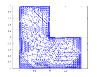
Figure 5.1: Adaptively generated NVB mesh on the L-shaped domain.

We consider the L-shaped domain $\Omega=(-1,1)^{2}\backslash[0,1]^{2}$ as depicted in Figure 5.1 and discretize (2.3) by piecewise linear functions in $S^{1,1}_{0}({\mathcal{T}}_{\ell})$ on adaptively generated NVB meshes ${\mathcal{T}}_{\ell}$ that are generated by the adaptive algorithm proposed in [FMP19]. This adaptive algorithm is steered by local error indicators given by

$$\eta_{\ell}=\left(\sum_{T\in{\mathcal{T}}_{\ell}}\left\|\widetilde{h}_{\ell}^{s}\big{(}f-(-\Delta)^{s}u_{\ell}\big{)}\right\|_{L^{2}(T)}^{2}\right)^{1/2}\!,\quad\text{with}\quad\widetilde{h}_{\ell}^{s}:=\begin{cases}h_{\ell}^{s}\quad&\text{for $0<s\leq 1/2$},\\ h_{\ell}^{1/2}w_{\ell}^{s-1/2}&\text{for $1/2<s<1$,}\end{cases}$$

where $u_{\ell}$ is the solution of (2.9). We note that by [FMP19, Theorem 2.3] theses indicators are reliable and for $s<1/2$ efficient in some weak sense. Moreover, [FMP19, Theorem 2.6] proves optimal convergence rates for the adaptive algorithm based on these estimators. Our implementation of the classical SOLVE-ESTIMATE-MARK-REFINE adaptive algorithm uses the MATLAB code from [ABB17] for the module SOLVE and adapted the MATLAB code for the local multilevel preconditioner from [FFPS17] to our model problem. Figure 5.2 gives the estimated condition numbers for the Galerkin matrix $\mathbf{A}^{L}$ and the preconditioned matrix $\widetilde{\mathbf{P}}_{AS}^{L}$, where the condition number has been estimated using power iteration and inverse power iteration (with random initial vectors) to compute approximations to the smallest and largest eigenvalues.

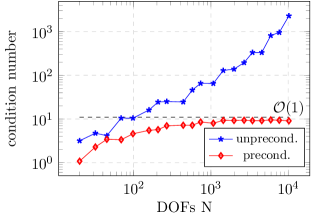
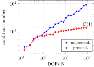
Figure 5.2: Estimated condition numbers for the unpreconditioned matrix $\mathbf{A}^{L}$ and the preconditioned matrix $\mathbf{P}_{AS}^{L}$ left: $s=0.25$, right: $s=0.75$.

We observe that, as expected, the condition number of the preconditioned system grows with the problem size, whereas the preconditioner leads to uniformly bounded condition numbers for the preconditioned system.

As the preconditioner is structurally similar to the one used in [FFPS17] for the hypersingular integral equation, we refer to the numerical results there for the confirmation that the preconditioner can also be realized efficiently.

References

- [ABB17] G. Acosta, F.M. Bersetche, and J.P. Borthagaray, A short FE implementation for a 2d homogeneous Dirichlet problem of a fractional Laplacian, Comput. Math. Appl. 74 (2017), no. 4, 784–816.
- [Aco01] G. Acosta, Lagrange and average interpolation over 3D anisotropic elements, J. Comput. Appl. Math. 135 (2001), no. 1, 91–109.
- [AF03] R.A. Adams and J.J.F. Fournier, Sobolev spaces, second ed., Pure and Applied Mathematics (Amsterdam), vol. 140, Elsevier/Academic Press, Amsterdam, 2003.
- [AFF+15] M. Aurada, M. Feischl, T. Führer, M. Karkulik, and D. Praetorius, Energy norm based error estimators for adaptive BEM for hypersingular integral equations, Appl. Numer. Math. 95 (2015), 15–35.
- [AFK+13] M. Aurada, M. Feischl, J. Kemetmüller, M. Page, and D. Praetorius, Each -stable projection yields convergence and quasi-optimality of adaptive FEM with inhomogeneous Dirichlet data in , ESAIM Math. Model. Numer. Anal. 47 (2013), no. 4, 1207–1235.
- [AG17] M. Ainsworth and C. Glusa, Aspects of an adaptive finite element method for the fractional Laplacian: a priori and a posteriori error estimates, efficient implementation and multigrid solver, Comput. Methods Appl. Mech. Engrg. 327 (2017), 4–35.
- [AL09] M. Arioli and D. Loghin, Discrete interpolation norms with applications, SIAM J. Numer. Anal. 47 (2009), no. 4, 2924–2951.
- [AM03] M. Ainsworth and W. McLean, Multilevel diagonal scaling preconditioners for boundary element equations on locally refined meshes, Numerische Mathematik 93 (2003), no. 3, 387–413.
- [AMT99] M. Ainsworth, W. McLean, and T. Tran, The conditioning of boundary element equations on locally refined meshes and preconditioning by diagonal scaling, SIAM J. Numer. Anal. 36 (1999), no. 6, 1901–1932.
- [Ape99a] T. Apel, Anisotropic finite elements: Local estimates and applications, Advances in Numerical Mathematics, Teubner, 1999.
- [Ape99b] T. Apel, Interpolation of non-smooth functions on anisotropic finite element meshes, M2AN 33 (1999), no. 6, 1149–1185.
- [Bad12] S. Badia, On stabilized finite element methods based on the Scott-Zhang projector. Circumventing the inf-sup condition for the Stokes problem, Comput. Methods Appl. Mech. Engrg. 247/248 (2012), 65–72.
- [BBN+18] A. Bonito, J.P. Borthagaray, R.H. Nochetto, E. Otárola, and A.J. Salgado, Numerical methods for fractional diffusion, Comput. Vis. Sci. 19 (2018), no. 5-6, 19–46.
- [BG98] C. Bernardi and V. Girault, A local regularization operator for triangular and quadrilateral finite elements, SIAM J. Numer. Anal. 35 (1998), no. 5, 1893–1916 (electronic).
- [BLN19] J.P. Borthagaray, W. Li, and R.H. Nochetto, Linear and nonlinear fractional diffusion, arXiv preprint arXiv:1906.04230 (2019).
- [BPV00] J.H. Bramble, J.E. Pasciak, and P.S. Vassilevski, Computational scales of Sobolev norms with application to preconditioning, Math. Comp. 69 (2000), no. 230, 463–480.
- [BPX91] J. Bramble, J. Pasciak, and J. Xu, Parallel multilevel preconditioners, Math. Comp. 55 (1991), 1–22.
- [BS02] S.C. Brenner and L.R. Scott, The mathematical theory of finite element methods, second ed., Texts in Applied Mathematics, vol. 15, Springer-Verlag, New York, 2002.
- [Car99] C. Carstensen, Quasi-interpolation and a posteriori error analysis in finite element methods, M2AN Math. Model. Numer. Anal. 33 (1999), no. 6, 1187–1202.
- [CH09] C. Carstensen and J. Hu, Hanging nodes in the unifying theory of a posteriori finite element error control, J. Comput. Math. 27 (2009), no. 2-3, 215–236.
- [Cia78] P.G. Ciarlet, The finite element method for elliptic problems, North-Holland Publishing Co., Amsterdam-New York-Oxford, 1978, Studies in Mathematics and its Applications, Vol. 4.
- [Cia13] P. Ciarlet, Jr., Analysis of the Scott-Zhang interpolation in the fractional order Sobolev spaces, J. Numer. Math. 21 (2013), no. 3, 173–180.
- [Coh03] A. Cohen, Numerical analysis of wavelet methods, Studies in Mathematics and its Applications, vol. 32, North-Holland Publishing Co., Amsterdam, 2003.
- [CS07] L. Caffarelli and L. Silvestre, An extension problem related to the fractional Laplacian, Comm. Partial Differential Equations 32 (2007), no. 7-9, 1245–1260.
- [DFG+04] W. Dahmen, B. Faermann, I. Graham, W. Hackbusch, and S. Sauter, Inverse inequalities on non-quasi-uniform meshes and application to the mortar element method, Mathematics of computation 73 (2004), no. 247, 1107–1138.
- [DKS16] L. Diening, C. Kreuzer, and R. Stevenson, Instance optimality of the adaptive maximum strategy, Found. Comput. Math. 16 (2016), no. 1, 33–68.
- [DL93] R.A. DeVore and G.G. Lorentz, Constructive approximation, Grundlehren der Mathematischen Wissenschaften [Fundamental Principles of Mathematical Sciences], vol. 303, Springer-Verlag, Berlin, 1993.
- [Dör96] W. Dörfler, A convergent adaptive algorithm for Poisson’s equation, SIAM J. Numer. Anal. 33 (1996), no. 3, 1106–1124.
- [DW91] M. Dryja and O.B. Widlund, Multilevel additive methods for elliptic finite element problems, Parallel algorithms for partial differential equations (Kiel, 1990), Notes Numer. Fluid Mech., vol. 31, Friedr. Vieweg, Braunschweig, 1991, pp. 58–69.
- [EG17] A. Ern and J.-L. Guermond, Finite element quasi-interpolation and best approximation, ESAIM Math. Model. Numer. Anal. 51 (2017), no. 4, 1367–1385.
- [FFPS17] M. Feischl, T. Führer, D. Praetorius, and E.P. Stephan, Optimal additive Schwarz preconditioning for hypersingular integral equations on locally refined triangulations, Calcolo 54 (2017), no. 1, 367–399.
- [FMP19] M. Faustmann, J.M. Melenk, and D. Praetorius, Quasi-optimal convergence rate for an adaptive method for the integral fractional laplacian, arXiv preprint arXiv:1903.10409 (2019).
- [FW15] R.S. Falk and R. Winther, The bubble transform: A new tool for analysis of finite element methods, Found. Comput. Math. (2015), 1–32 (English).
- [GS02] V. Girault and L. R. Scott, Hermite interpolation of nonsmooth functions preserving boundary conditions, Math. Comp. 71 (2002), no. 239, 1043–1074 (electronic).
- [GSUT19] H. Gimperlein, J. Stocek, and C. Urzúa-Torres, Optimal operator preconditioning for pseudodifferential boundary problems, arXiv preprint arXiv:1906.09164 (2019).
- [Hip06] R. Hiptmair, Operator preconditioning, Comput. Math. Appl. 52 (2006), no. 5, 699–706.
- [KM15] M. Karkulik and J.M. Melenk, Local high-order regularization and applications to -methods, Comput. Math. Appl. 70 (2015), no. 7, 1606–1639.
- [KPP13] M. Karkulik, D. Pavlicek, and D. Praetorius, On 2D newest vertex bisection: optimality of mesh-closure and -stability of -projection, Constr. Approx. 38 (2013), no. 2, 213–234.
- [LMWZ10] J. Li, J.M. Melenk, B. Wohlmuth, and J. Zou, Optimal a priori estimates for higher order finite elements for elliptic interface problems, Appl. Numer. Math. 60 (2010), no. 1-2, 19–37.
- [Mai09] M. Maischak, A multilevel additive Schwarz method for a hypersingular integral equation on an open curve with graded meshes, Appl. Numer. Math. 59 (2009), no. 9, 2195–2202.
- [MN85] A.M. Matsokin and S.V. Nepomnyaschikh, A schwarz alternating method in a subspace, Soviet Math. 29 (1985), no. 10, 78–84.
- [Osw94] P. Oswald, Multilevel finite element approximation, Teubner Skripten zur Numerik, Teubner, 1994.
- [Ran12] A. Rand, Average interpolation under the maximum angle condition, SIAM J. Numer. Anal. 50 (2012), no. 5, 2538–2559.
- [Sch98] R. Schneider, Multiskalen- und Wavelet-Matrixkompression, Advances in Numerical Mathematics, B. G. Teubner, Stuttgart, 1998, Analysisbasierte Methoden zur effizienten Lösung großer vollbesetzter Gleichungssysteme. [Analysis-based methods for the efficient solution of large nonsparse systems of equations].
- [Ste08] R. Stevenson, The completion of locally refined simplicial partitions created by bisection, Math. Comp. 77 (2008), no. 261, 227–241.
- [SvV19] R. Stevenson and R. van Veneti, Uniform preconditioners for problems of positive order, arXiv preprint arXiv:1906.09164 (2019).
- [SZ90] L.R. Scott and S. Zhang, Finite element interpolation of nonsmooth functions satisfying boundary conditions, Math. Comp. 54 (1990), no. 190, 483–493.
- [Tar07] L. Tartar, An introduction to Sobolev spaces and interpolation spaces, Lecture Notes of the Unione Matematica Italiana, vol. 3, Springer, Berlin, 2007.
- [TS96] T. Tran and E.P. Stephan, Additive Schwarz methods for the -version boundary element method, Appl. Anal. 60 (1996), no. 1-2, 63–84.
- [TSM97] T. Tran, E.P. Stephan, and P. Mund, Hierarchical basis preconditioners for first kind integral equations, Appl. Anal. 65 (1997), no. 3-4, 353–372.
- [TSZ98] T. Tran, E.P. Stephan, and S. Zaprianov, Wavelet-based preconditioners for boundary integral equations, vol. 9, 1998, Numerical treatment of boundary integral equations, pp. 233–249.
- [TW05] A. Toselli and O. Widlund, Domain decomposition methods—algorithms and theory, Springer Series in Computational Mathematics, vol. 34, Springer-Verlag, Berlin, 2005.
- [Zha92] X. Zhang, Multilevel Schwarz methods, Numer. Math. 63 (1992), 521–539.