Properties of OB star$-$black hole systems derived from detailed binary evolution models

Abstract

Context. The recent gravitational wave measurements have demonstrated the existence of stellar mass black hole binaries. It is essential for our understanding of massive star evolution to identify the contribution of binary evolution to the formation of double black holes.

Aims. A promising way to progress is investigating the progenitors of double black hole systems and comparing predictions with local massive star samples such as the population in 30 Doradus in the Large Magellanic Cloud (LMC).

Methods. To this purpose, we analyse a large grid of detailed binary evolution models at LMC metallicity with initial primary masses between 10 and 40$\,\mathrm{M}_{\odot}$, and identify which model systems potentially evolve into a binary consisting of a black hole and a massive main sequence star. We then derive the observable properties of such systems, as well as peculiarities of the OB star component.

Results. We find that $\sim$3% of the LMC late O and early B stars in binaries are expected to possess a black hole companion, when assuming stars with a final helium core mass above $6.6\,\mathrm{M}_{\odot}$ to form black holes. While the vast majority of them may be X-ray quiet, our models suggest that these may be identified in spectroscopic binaries, either by large amplitude radial velocity variations ($\mathrel{\hbox{\hbox to0.0pt{\hbox{\lower 4.0pt\hbox{$\sim$}}\hss}\hbox{$>$}}}50\,{\rm km}\,{\rm s}^{-1}$) and simultaneous nitrogen surface enrichment, or through a moderate radial velocity ($\mathrel{\hbox{\hbox to0.0pt{\hbox{\lower 4.0pt\hbox{$\sim$}}\hss}\hbox{$>$}}}10\,{\rm km}\,{\rm s}^{-1}$) and simultaneously rapid rotation of the OB star. The predicted mass ratios are such that main sequence companions could be excluded in most cases. A comparison to the observed OB+WR binaries in the LMC, Be/X-ray binaries, and known massive BH binaries supports our conclusion.

Conclusions. We expect spectroscopic observations to be able to test key assumptions in our models, with important implications for massive star evolution in general, and for the formation of double-black hole mergers in particular.

1 Introduction

Massive stars play a central role in astrophysics. They dominate the evolution of star-forming galaxies by providing chemical enrichment, ionising radiation and mechanical feedback (e.g., Mac Low & Klessen 2004, Hopkins et al., 2014, Crowther et al. 2016). They also produce spectacular and energetic transients, ordinary and superluminous supernovae, and long-duration gamma-ray bursts (Smartt 2009, Fruchter et al. 2006, Quimby et al. 2011), which signify the birth of neutron stars and black holes (Heger et al. 2003, Metzger et al. 2017).

Massive stars are born predominantly as members of binary and multiple systems (Sana et al. 2012, 2014, Kobulnicky et al. 2014, Moe & Di Stefano 2017). As a consequence, most of them are expected to undergo strong binary interaction, which drastically alters their evolution (Podsiadlowski et al., 1992, Van Bever & Vanbeveren 2000, O’Shaughnessy et al. 2008, de Mink et al. 2013). On the one hand, the induced complexity is a reason that many aspects of massive star evolution are yet not well understood (Langer 2012, Crowther 2020). On the other hand, the observations of binary systems provide excellent and unique ways to determine the physical properties of massive stars (Hilditch et al. 2005, Torres et al. 2010, Pavlovski et al. 2018, Mahy et al. 2020) and to constrain their evolution (Ritchie et al. 2010, Clark et al. 2014. Abdul-Masih et al. 2019a).

Gravitational wave astronomy has just opened a new window toward understanding massive star evolution. Since the first detection of cosmic gravitational waves on September 14, 2015 (Abbott et al. 2016), reports about the discovery of such events have become routine (Abbott et al. 2019), with a current rate of $\sim$1 per week. Most of these sources correspond to merging stellar mass black holes with high likelihood (cf., https://gracedb.ligo.org/latest/). It is essential to explore which fraction of these gravitational wave sources reflects the end product of massive close binary evolution, compared to products of dynamical (Kulkarni et al. 1993, Sigurdsson & Hernquist 1993, Antonini et al. 2016, Samsing & D’Orazio 2018, Fragione et al. 2019, Di Carlo et al. 2019) and primordial (Nishikawa et al. 2019) formation paths.

Two different evolutionary scenarios for forming compact double black hole binaries have been proposed. The first one involves chemically homogeneous evolution (Maeder 1987, Langer 1992, Yoon & Langer 2005), which may lead to the avoidance of mass transfer in very massive close binaries (de Mink et al. 2009) and allows compact main sequence binaries to directly evolve into compact black hole binaries (Mandel & de Mink 2016). This scenario has been comprehensively explored through detailed binary evolution models (Marchant et al. 2016), showing that it leads to double black hole mergers only at low metallicity ($Z\mathrel{\hbox{\hbox to0.0pt{\hbox{\lower 4.0pt\hbox{$\sim$}}\hss}\hbox{$<$}}}Z_{\odot}/10$), and is restricted to rather massive black holes ($\mathrel{\hbox{\hbox to0.0pt{\hbox{\lower 4.0pt\hbox{$\sim$}}\hss}\hbox{$>$}}}30\,\mathrm{M}_{\odot}$; see also de Mink & Mandel 2016).

The second proposed path towards the formation of compact double black hole binaries is more complex, and involves mass transfer due to Roche-lobe overflow and common envelope evolution (Belczynski et al. 2016, Kruckow et al. 2018). At the same time, this path predicts a wide range of parameters for the produced double compact binaries, i.e., it resembles those suggested for forming merging double neutron stars (e.g., Bisnovatyi-Kogan & Komberg 1974, Flannery & van den Heuvel 1975, Tauris et al. 2017), double white dwarfs (Iben & Tutokov 1984, Webbink 1984) and white dwarf-neutron star binaries (Toonen et al. 2018). Although this type of scenario has not been verified through detailed binary evolution models, there is little doubt that the majority of objects in the observed populations of close double white dwarfs (Breedt et al. 2017, Napiwotzki et al. 2020) and double neutron stars (Tauris et al. 2017, Stovall et al. 2018, Andrews & Zezas 2019) have been evolving accordingly. Consequently, we may expect that also close double black holes from in a similar way.

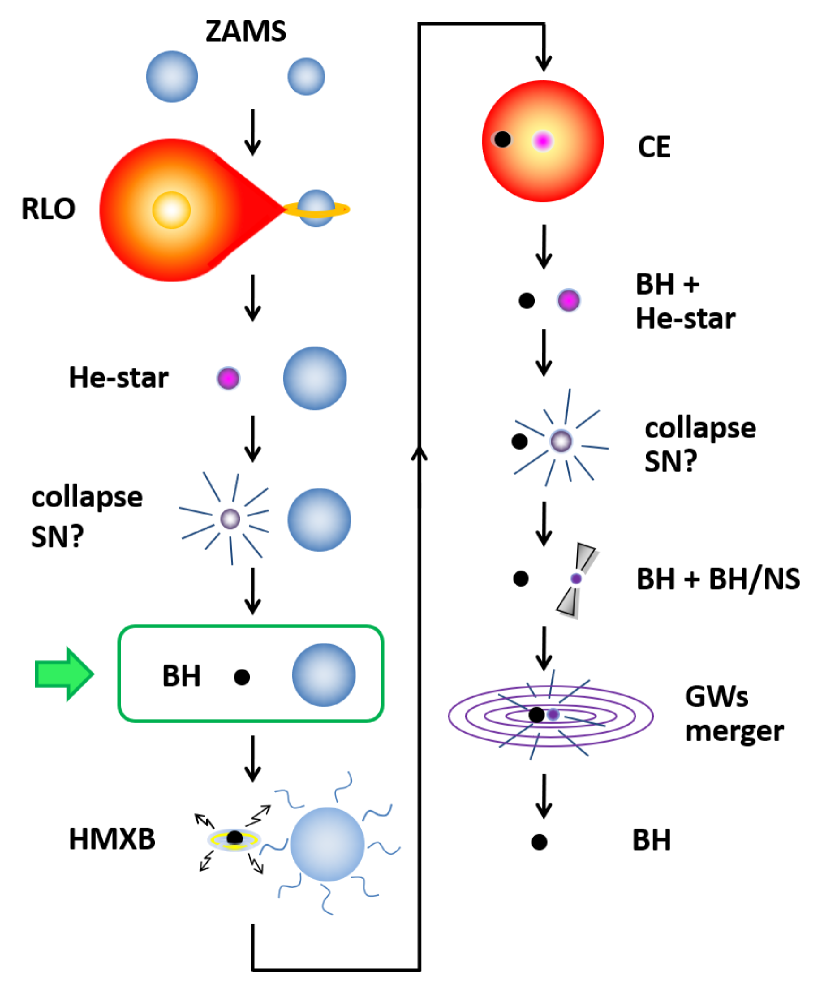
Figure 1: Schematic evolutionary path for the formation of compact BH-NS systems. Acronyms used in this figure: ZAMS: zero-age main sequence; RLO: Roche-lobe overflow (mass transfer); He-star: helium star (could be a Wolf-Rayet star, if sufficiently massive); SN: supernova; BH: black hole; HMXB: high-mass X-ray binary; CE: common envelope; NS: neutron star. Light green highlights the OB+BH stage, which is the focus of this paper. Adapted from Krokow et al. (2018).

Figure 1 gives an example for the schematic formation path of double compact binaries (Kruckow et al. 2018). It involves several stages for which current theoretical predictions are very uncertain, most notably those of Roche-lobe overflow, common envelope evolution, and black hole formation. Evidently, it is desirable to obtain observational tests for as many as possible of the various involved evolutionary stages. For this, it is important to realise that in many of the steps which are shown in Fig. 1, a large fraction of the binary systems may either merge or break up, such that the birth rate of double compact systems at the end of the path is several orders of magnitude smaller than that of the double main sequence binaries at the beginning of the path. Observational tests may therefore be easier for the earlier stages, where we expect many more observational counter parts.

Here, the OB+BH stage, where a BH orbits an O or early B-type star, has a prominent role, concerning theory and observations. From the theoretical perspective, it is the last long-lived stage which can be reached from the double main sequence stage with detailed stellar evolution calculation. Whereas the preceding Roche-lobe overflow phase also bears large uncertainties, it can be modeled by solving the differential equations of stellar structure and evolution, rather than having to rely on simple recipes for the structure of the two stars. At the same time, the number of main sequence binaries that are expected to merge during the first Roche-lobe overflow phase is typically only about half, such that the number of OB+BH binaries is expected to be significant.

In this paper, we describe the properties of OB+BH binaries as obtained from a large grid of detailed binary evolution models. In Sect. 2, we explain which method was used to obtain our results. Our Sect. 3 focuses on the derived distributions of the properties of the OB+BH binaries, while Sect. 4 gives a discussion of the key uncertainties which enter our calculations. We compare our results with earlier work in Sect. 5, and provide a comparison with observations in Sect. 6. In Sect. 7, we discuss observational strategies for finding OB+BH binaries, and in Sect. 8, we consider their future evolution. We summarise our conclusions in Sect. 9.

2 Method

Our results are based on a dense grid of detailed massive binary evolution models (Marchant 2016). These models were computed with the stellar evolution code MESA (Modules for Experiments in Stellar Astrophysics, Version No. 8845) with a physics implementation as described by Paxton et al. (2015). All necessary files to reproduce our MESA simulations are available at https://doi.org/10.5281/zenodo.3698636.

In particular, differential rotation and magnetic angular momentum transport are included as in Heger et al. (2000, 2005), with physics parameters set as in Brott et al. (2011). Mass and angular momentum transfer is computed according to Langer et al. (2003) and Petrovic et al. (2005), and the description of tidal interaction follows Detmers et al. (2008). Convection is modeled according to the standard Mixing Length Theory (Böhm-Vitense 1958) with a mixing length parameter of $\alpha_{\rm MLT}=1.5$.

Semiconvection is treated as in Langer (1991), i.e., using $\alpha_{\rm SC}=0.01$. We note that recent evidence may favour higher values of this parameter, which could lead to a nuclear timescale post-main sequence expansion to the RSG stage of massive low-metallicity stars in a limited mass range (Schootemeijer et al. 2019, Higgins & Vink 2020, Klencki et al. 2020). The consequences of this for massive binary evolution will need to be explored (cf., Wang et al., 2020). It could lead to the prediction of a significant sub-population of Roche-lobe filling, X-ray bright, B- and A-type supergiant BH binaries (Quast et al. 2019, Klencki et al. 2020), which, especially at low metallicity, appears not to be observed. Clearly, more work is needed to clarify the situation.

Thermohaline mixing is performed as in Cantiello & Langer (2010), and convective core overshooting is applied with a step-function extending the cores by 0.335 pressure scale heights (Brott et al. 2011). However, overshooting is only applied to layers which are chemically homogeneous. This implies that mean molecular weight gradients are fully taken into account in the rejuvenation process of mass gaining main sequence stars (cf., Braun & Langer 1995). The models are computed with the same initial chemical composition as those of Brott et al. (2011), i.e., taking the non-Solar abundance ratios in the LMC into account. Differently from Brott et al., here custom-made OPAL opacities (Iglesias & Rogers 1996) in line with the adopted initial abundances have been produced and included in the calculations.

The masses of the primary stars range from 10 to 39.8$\,\mathrm{M}_{\odot}$ in steps of $\log\left(M_{1}/\,\mathrm{M}_{\odot}\right)=0.050$. For each primary mass, systems with different initial mass ratios $q_{i}=M_{2}/M_{1}$ ranging from 0.25 to 0.975, in intervals of 0.025 are computed and for each mass ratio, there are models with orbital periods from 1.41 to 3160 d in steps of $\log\left(P_{i}/{\rm d}\right)=0.025$. The grid consists of a total of 48240 detailed binary evolution models. Binaries with initial periods below $\sim 5\,$d (for a primary mass of 10$\,\mathrm{M}_{\odot}$) and $25\,$d (for a primary mass of 39.8$\,\mathrm{M}_{\odot}$) undergo mass transfer while both stars fuse hydrogen in their cores (Case A systems) while most larger period binaries undergo mass transfer immediately after the primary leaves the main sequence (Case B systems). For higher primary masses, envelope inflation due to the Eddington limit (Sanyal et al. 2015) would prevent stable Case B mass transfer to occur (cf., Sect. 4). Figure 2 gives an overview of the evolutionary end points obtained for models with an initial primary mass of $\sim 25.12\,\mathrm{M}_{\odot}$, with examples for other primary masses provided in Appendix B.

Our models are computed assuming tidal synchronisation at zero age, which avoids introducing the initial rotation rate of both stars as additional parameters. While this is not physically warranted, it is justified since moderate rotation is not affecting the evolution of the individual stars very much (Brott et al., 2011; Choi et al. 2016), and the fastest rotators may be binary evolution products (de Mink et al., 2013; Wang et al. 2020). Moreover, the initially closer binary models (typically those of Case A), evolve quickly into tidal locking (de Mink et al. 2009), independent of the initial stellar spins. Also the spins of the components of all post-interaction binaries, in particular those of the OB+BH binaries analysed here, are determined through the interaction process, where the mass donor fills its Roche-volume in synchronized rotation also in Case B systems, and the mass gainer is spun-up by the accretion process.

The evolution of our models is stopped if mass overflow at the outer Lagrangian point L2 occurs (purple color in Fig. 2) in contact binaries (black hatching in Fig. 2), which are otherwise modeled as in Marchant (2016). We further stop the evolution if inverse mass transfer occurs from a post main sequence component (yellow color in Fig. 2), or if a system exceeds the upper mass-loss rate limit (green color in Fig. 2). Any of these condition is assumed to lead to a merger. Here, the upper mass loss rate limit is set by the condition that the energy required to remove the emitted fraction of the transfered matter exceeds the radiated energy of both stars. Models surpassing the weaker condition that the momentum required to remove the non-accreted mass exceeds their photon momentum are assumed to survive as binaries. The systems are evolved at least until central helium depletion of the mass gainer, while those with helium core masses smaller than $13\,\mathrm{M}_{\odot}$ are followed until core carbon depletion.

In the systems with the largest initial orbital periods, the mass transfer rate grows on near-dynamical time scales to very large values, with a classical common envelope evolution to follow (red color in Fig. 2). In some systems, in particular those with the largest initial periods and the most massive secondary stars, a merger as consequence of the common envelope evolution may be avoided. Here, we assume that also these systems merge, such that the numbers and frequencies of OB+BH systems that we obtain below must be considered as lower limits. The systems which survive a common envelope evolution would likely contribute to the shortest period OB+BH binaries. As such, they would likely evolve into an OB star-BH merger later-on, and not contribute to the production of double compact binaries. More details about the binary evolution grid can be found in Marchant (2016).

An inspection of the detailed results showed that some of the contact systems were erroneous. In these cases, the primary kept expanding after contact was reached, but no mass transfer was computed. This situation is unphysical. An example case is the model with the initial parameters $(\log M_{\rm 1,i},q_{\rm i},\log P_{\rm orb,i})=(1.4,0.4,0.2)$. In Fig. 2, this concerns the 10 blue pixel inside the frame in the lower right corner. The error lead to these systems surviving until, including, the OB+BH stage. The error did not occur for initial mass ratios above 0.5. In a recalculation of several of the erroneous systems with MESA Version No. 12115, the unphysical situation did not occur. In these calculations, the systems merged while both stars underwent core hydrogen burning. In order to avoid any feature of the erroneous models in our results for OB+BH binaries, we disregard by hand binary models for which simultaneously $q_{\rm i}<0.55$ and $\log P_{\rm orb,i}<0.5$, such that none of the non-erroneous systems in this part of the parameter space contributes to the OB+BH binary population. These systems remain to be considered duing their pre-interaction evolution.

To account for OB+BH systems, we assess the helium core masses of our models. We consider the pre-collapse single star models of of Sukhbold et al. (2018), who evaluate the explodability of their models based on their so-called compactness parameter (O’Connor & Ott 2011, Ugliano et al. 2012). Near an initial mass of 20$\,\mathrm{M}_{\odot}$, this parameter shows a sudden increase, with most stellar models below this mass providing supernovae and neutron stars, and most models above this mass expected to form BHs. This mass threshold is essentially confirmed by Ertl et al. (2016) and Müller et al. (2016) based on different criteria, and corresponds to a final helium core mass of 6.6$\,\mathrm{M}_{\odot}$, and a final CO-core mass of 5$\,\mathrm{M}_{\odot}$ (Sukhbold et al. 2018). Sukhbold et al. also find the threshold to depend only weakly on metallicity. Whereas these three papers all predict a non-monotonous behaviour as function of the initial mass, with the possibility of some successful supernovae occurring above 20$\,\mathrm{M}_{\odot}$, we neglect this possibility for simplicity, and assume BHs to form in models with a helium core mass above 6.6$\,\mathrm{M}_{\odot}$ at the time of core carbon exhaustion.

While our adopted BH formation criterion is based on single stars, it has been argued that in stripped stars, the helium core does not grow in mass during helium burning, such that the ${}^{12}C$-abundance remains larger, which ultimately leads to a higher likelihood for NS production than in corresponding single stars (Brown et al. 2001). On the other hand, recent pre-collapse models evolved from helium stars (Woosley 2019) show a similar jump of the compactness parameter as quoted above. The onset of this jump is shifted to larger helium core masses by about 0.5$\,\mathrm{M}_{\odot}$, while the peak is shifted by $\sim 2\,\mathrm{M}_{\odot}$. Also, the helium star models predict an island of low compactness in the He-core mass range $10\dots 12\,\mathrm{M}_{\odot}$ which is absent or much reduced in the models which are clothed with a H-rich envelope. Therefore, with our BH formation criterion as mentioned above, we may overpredict relatively low-mass black holes. We discuss the corresponding uncertainty in Sect.4.

We further assume that the mass of the BH is the same as the mass of the He-core of its progenitor, and that the BHs form without a momentum kick. The validity of these assumptions depends on the amount of neutrino energy injection into the fall-back material after core bounce (Batta et al. 2017). In the direct collapse scenario, the BH forms very quickly, and a strong kick and mass ejection from the helium star may be avoided. However, in particular near the NS/BH formation boundary, both assumptions may be violated to some extent. This introduces some additional uncertainty for our model predictions in the lower part of the BH mass range (cf., Sect.4)

Due to the high density of our binary evolution grid, it is well suited to construct synthetic stellar populations. In order to do so, sets of random initial binary parameters are defined under the condition that they obey chosen initial distribution functions. This is done here by requiring that the primary masses follow the Salpeter (1955) initial mass function, and that the initial mass ratios and orbital periods follow the distributions obtained by Sana et al. (2013, see also Almeida et al. 2017) for the massive stars observed in the VLT FLAMES Tarantula survey (Evans et al. 2011). The adopted IMF should serve to constrain the lower limits on the number of systems (cf. adopting the shallower value for the 30 Doradus region from Schneider et al. 2018).

One may select models at a predefined age to construct synthetic star clusters (cf., Wang et al. 2020), or, as done here, consider a constant star formation rate. We then consider a given binary model an OB+BH system if it fulfills our BH formation criterion for the initially more massive star, and if the initially less massive star is still undergoing core hydrogen burning ($X_{\rm c}\geq 0.01$). We then consider its statistical weight in accordance with the above mentioned distribution functions, and its lifetime as OB+BH binary. With this taken into account, its properties are evaluated at the time of BH formation.

Figure 2: Outcome of the 4020 binary evolution models with an initial primary mass of $\log M/\,\mathrm{M}_{\odot}=1.4$ ($\sim 25.12\,\mathrm{M}_{\odot}$), as function of their initial orbital period $P_{\rm i}$ and mass ratio $q_{\rm i}$. Each of the $30\times 134$ pixel in this plot represents one detailed binary evolution model. The dark blue systems evolve to the OB+BH stage. Systems that evolve into a contact configuration are marked by black hatching. Purple color indicates systems evolving into mass overflow at the outer Lagrangian point L2, and systems evolving into inverse mass transfer occuring from a post main sequence component are marked in yellow; we assume the binaries merge in both situations. We also assume those systems to merge which exceed the upper mass-loss rate limit (see main text), marked in green. The systems with the largest initial orbital periods, marked in red, impart a classical common envelope evolution; for simplicity, we assume all of them to merge as well. Systems below the nearly horizontal white line undergo the first mass transfer while both stars are core hydrogen burning (Case A), while the primaries in initially wider systems starts mass transfer after core hydrogen exhaustion (Case B). The area framed by the black line in the lower right corner marks the part of the parameter space which is disregarded in our results (see Sect. 2). Equivalent plots for four more initial primary masses are provided in the Appendix.

3 Results

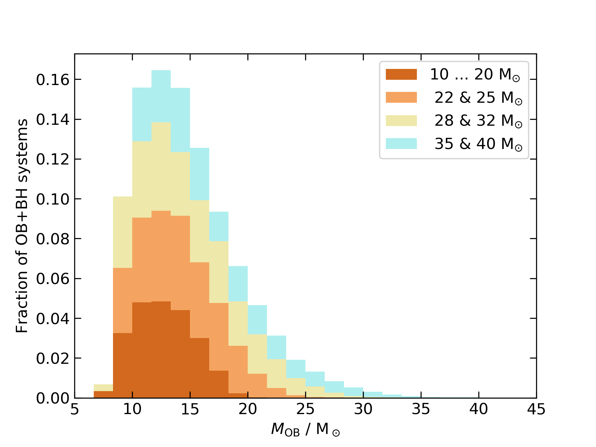
Figure 3: Top: Distribution of the OB star masses of systems in our binary evolution model grid that reach the OB+BH stage, assuming constant star formation, weighted with the IMF and the initial binary parameter distribution functions, and with their lifetime as OB+BH binary. The red and blue areas represent Case B and Case A systems. Black colour indicates the small number of non-interacting systems in our binary grid. The results are stacked, such that the upper envelope corresponds to the total number of systems. The ordinate values are normalised such that the value for each bin gives its relative contribution to the total number of systems. Bottom: the same distribution as in the top plot, but discriminating between different initial masses of the BH prigenitors (see legend).

As we focus on the properties of OB+BH binaries in this paper, in the following we discuss only systems that avoid to merge before they form the first compact object. In that, it is useful to consider the Case A systems separately from the Case B systems. Not only are the predictions from both classes of binaries quite distinct from each other (see below), but also the physics which is involved in the mass transfer process.

To a large extent, tidal effects can be neglected in the wider Case B systems, while they play an important role in Case A systems. In the latter, tidal coupling slows down or prevents the spin-up of the mass gainer during mass transfer, while direct impact accretion also reduces the specific angular momentum of the accreted matter (Langer 2012). Consequently, the mass transfer efficiency, i.e., the ratio of the mass accreted by the mass gainer over the amount of transferred mass, can be high in Case A systems. We find accretion efficiencies of up to nearly one, with an average of about 30% for all Case A binaries, and the highest values are achieved for the most massive systems and largest initial mass ratios (i.e., $q\simeq 1$). In contrast, the mass transfer is rather inefficient in most of our Case B systems, because the mass gainer is quickly spun-up to critical rotation, such that any further accretion remains very limited. The overall accretion efficiency remains at the level of 10% or less.

3.1 OB star masses, BH masses, mass ratios

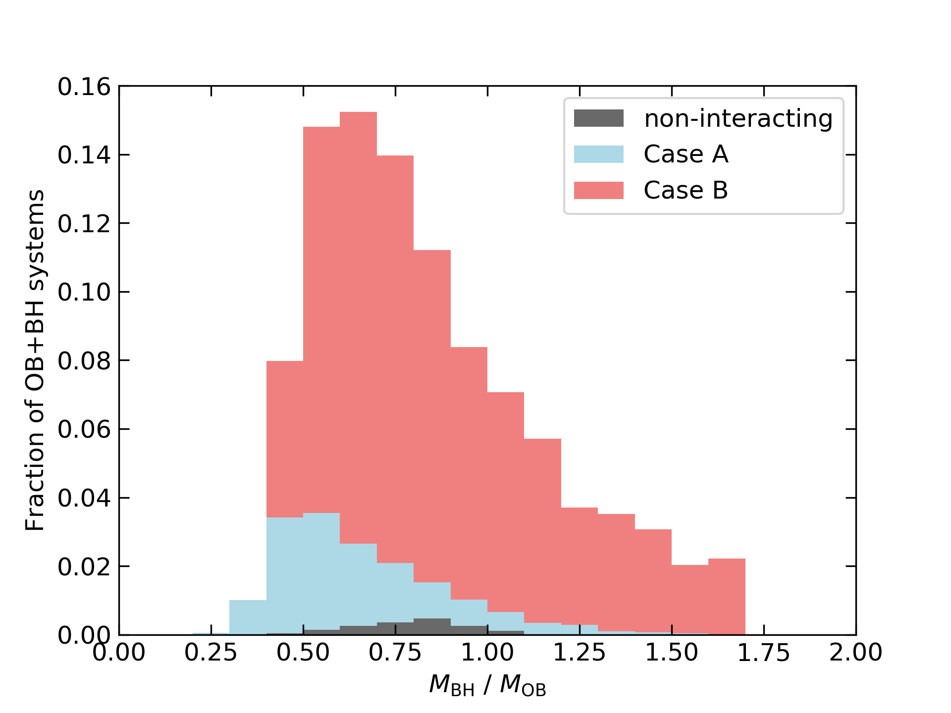
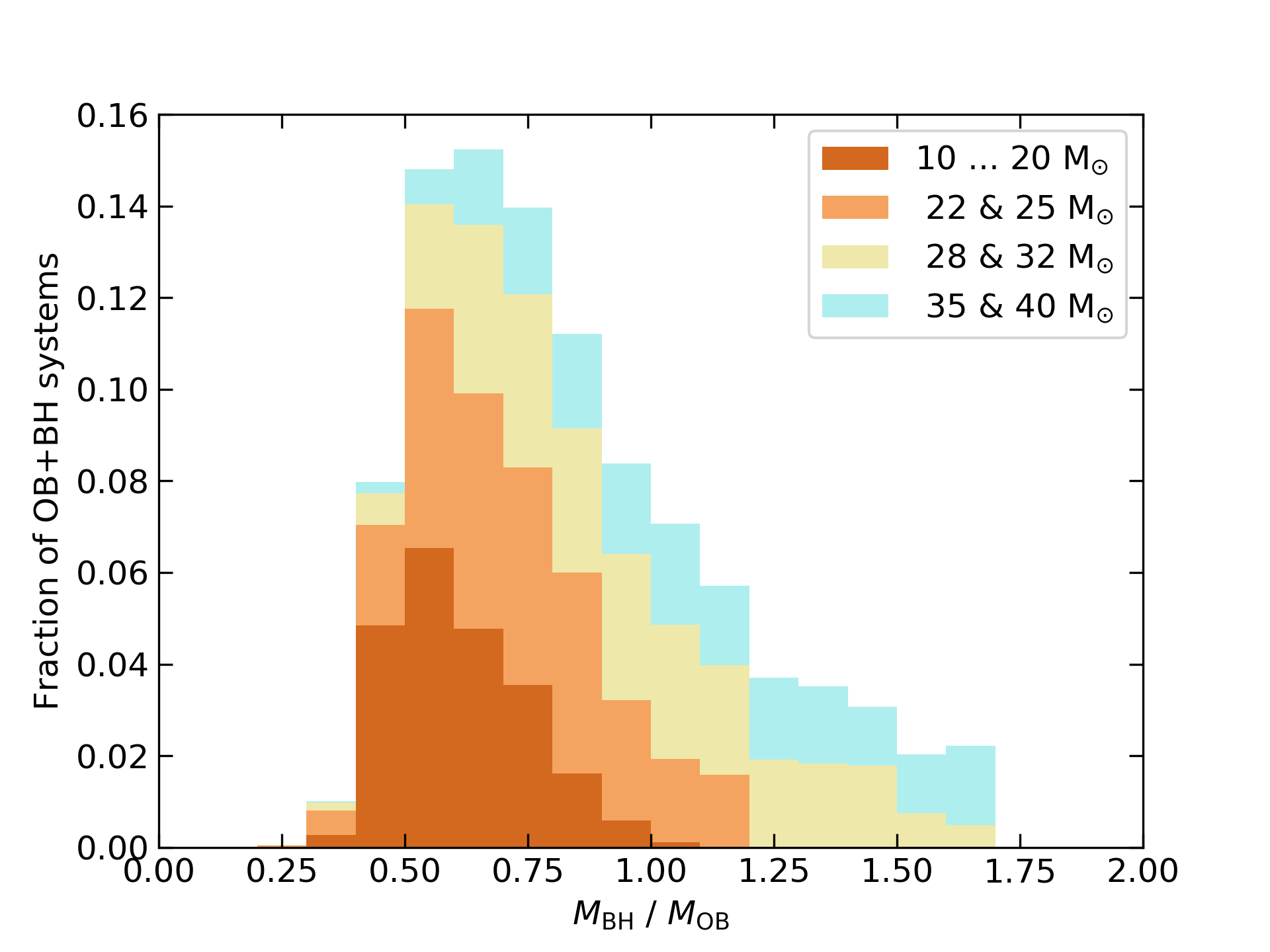
Figure 4: Top: As Fig. 3, here showing the distribution of the BH/OB-star mass ratios in our predicted OB+BH binaries. Bottom: the same distribution as in the top plot, but discriminating between different initial masses of the BH progenitors (see legend).

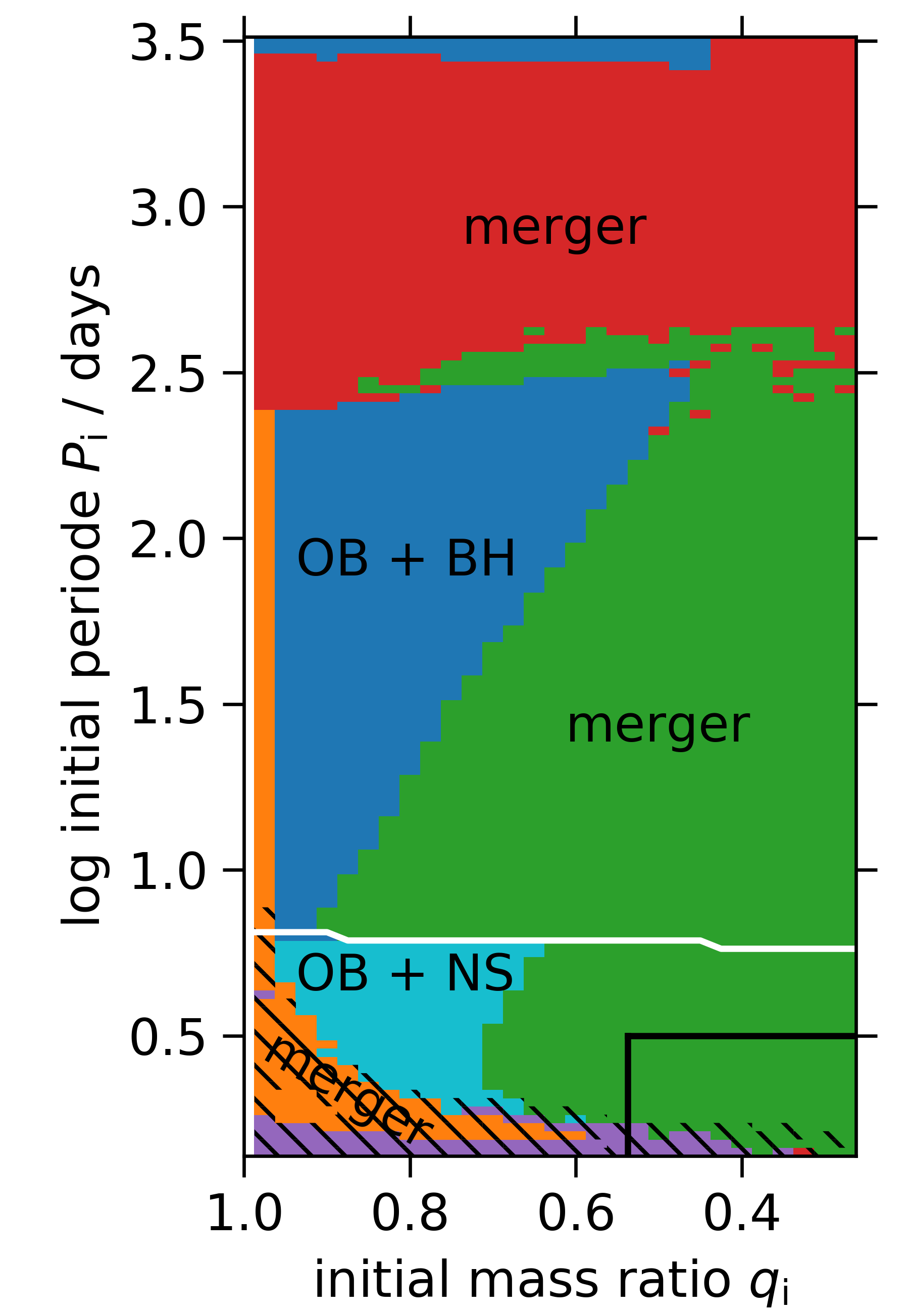
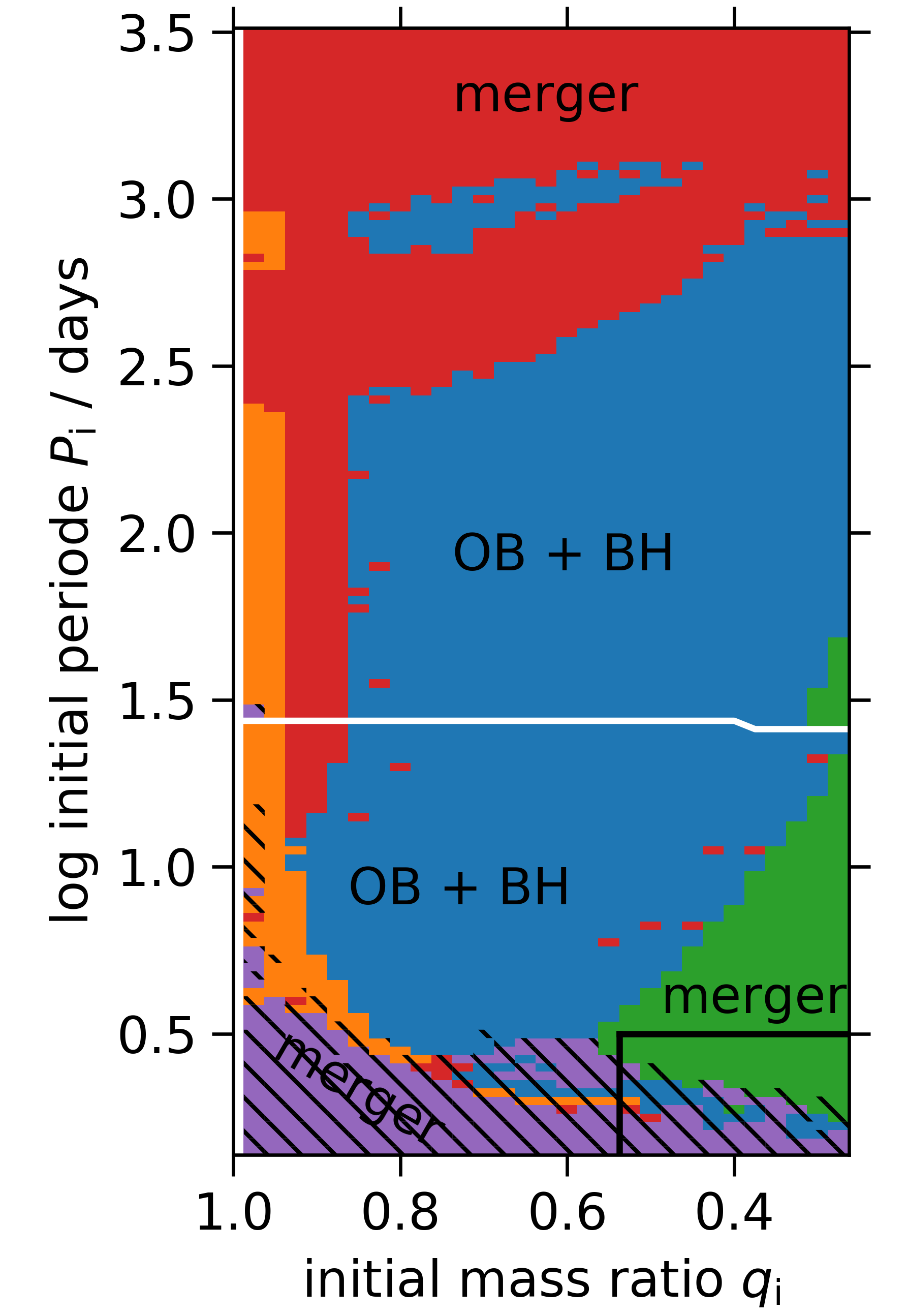
Figure 14: As Fig. 2, but for initial primary masses of $15.85\,\mathrm{M}_{\odot}$ (top left), $17,17\,\mathrm{M}_{\odot}$ (top right), 19.19$\,\mathrm{M}_{\odot}$ (bottom left) and 39.81$\,\mathrm{M}_{\odot}$ (bottom right). The color coding indicates fates as in Fig. 2 (purple: L2-overflow, yellow: inverse mass transfer, green: mass loss limit violation, red: common envelope evolution; all assumed to lead to a merger). Black hatching marks contact evolution, and the dark blue systems evolve to the OB+BH stage. Here, the light blue color marks systems where the mass donor is assumed to form a neutron star rather than a black hole. The white line separates Case A and Case B evolution, and the area framed by the black line in the lower right corner marks the part of the parameter space which is disregarded in our results (see Sect. 2).

As found in previous binary evolution calculations (e.g., Yoon et al., 2010), the mass donors of our model binaries are stripped of nearly their entire hydrogen envelope as consequence of Roche-lobe overflow. Whereas small amounts of hydrogen may remain in the lower-mass primaries (Gilkis et al., 2019), it is reasonable to consider them as helium stars after the mass transfer phase. Whereas the initial helium star mass emerging from Case B binaries is very similar to the initial helium core mass (i.e., at core helium ignition) of single stars, we emphasise that, due to larger amounts of mass being transferd during the MS stage, Case A binaries produce significantly smaller mass helium stars (cf., fig. 14 of Wellstein et al., 2001), an effect which is mostly not accounted for in simplified binary evolution models.

Figure 3 evaluates the distribution of the masses of the OB stars in our OB+BH models at the time of the formation of the first compact object. Besides the Case A and B systems, it distinguishes for completeness, the systems in our grid which never interact. The results shown in Fig. 3 are weighted by the initial mass and binary parameter distribution functions (see Sect. 2), and by the duration of the OB+BH phase of the individual binary models. As such, Fig. 3 predicts the measured distribution of the OB star masses in idealised and unbiased observations of OB+BH binaries.

The distribution of the masses of the OB stars in our OB+BH binaries shown in Fig. 3 has a peak near $14\,\mathrm{M}_{\odot}$. Towards lower OB masses, the chance that the final helium core mass of the mass donor falls below our threshold mass for BH formation is increasing. Whereas for the donor star initial masses, there is a cut-off near $18\,\mathrm{M}_{\odot}$ below which no BHs are produced, the distribution of the masses of their companions leads to a spread of the lower mass threshold of the secondaries, i.e., the OB stars in BH+OB systems, leading to the lowest masses of the BH companions of about $8\,\mathrm{M}_{\odot}$. The drop of the number of systems for OB star masses above $14\,\mathrm{M}_{\odot}$ is mainly produced by the initial mass function, and by the shorter lifetime of more massive OB stars. Due to the limits of our model grid to initial primary masses below $40\,\mathrm{M}_{\odot}$, we may be missing stars in the distribution shown in Fig. 3 above $\sim 20\,\mathrm{M}_{\odot}$. However, their contribution is expected to be small, and it is very uncertain since the corresponding stars show envelope inflation (cf., Sect. 4).

The upper panel of Fig. 3 shows that the majority of OB+BH systems is produced via Case B evolution, as expected from Fig. 2 when the areas covered by Case A and Case B in the $q_{\rm i}-P_{\rm i}$-plane are compared (though note that our initial distributions are not exactly flat in $\log P_{\rm i}$ and $q_{\rm i}$). The peak in the OB mass distribution of the Case A models is shifted to higher masses ($\sim 16\,\mathrm{M}_{\odot}$), compared to the Case B distribution due to the higher accretion efficiency in Case A. For the same reason, the most massive OB stars in the OB+BH systems produced by our grid, with masses of up to $47\,\mathrm{M}_{\odot}$, evolved via Case A (cf., Sect. 7). The Case B binaries produce only OB star companions to BHs with masses below $\sim 34\,\mathrm{M}_{\odot}$, notably since the most massive Case B systems with mass ratios above $\sim 0.9$ lead to mergers before the BH is formed.

The bottom panel of Fig. 3 provides some insight into the mass dependence of the production of OB+BH binaries (see also bottom panel of Fig. 4), by comparing the contributions from binary systems with four different initial primary mass ranges. We see that systems with successively more massive primaries produce more massive OB stars in OB+BH binaries. We also see that the range of OB star masses in OB+BH binaries originating from systems with more massive primaries is larger. This reflects our criterion for mergers in Case B systems (Sect. 2), which implies that it is easier for more massive binaries to drive the excess mass which the spun-up mass gainer can not accrete any more out of the system.

Figure 4 shows the resulting distribution of mass ratios of our OB+BH binary models, produced with the same assumptions as Fig. 3. Remarkably, the distribution drops sharply for BH/OB star mass ratios below 0.5. The main reason is that the BH is produced by the initially more massive star in the binary. This means that binaries with a small initial mass ratio (say $M_{\rm 2,i}/M_{\rm 1,i}\simeq 1/3$; cf., Fig. 2) easily produce black holes as massive as their companion or more, such that their BH/OB mass ratios is one or higher. Since the accretion efficiency in our models is mostly quite low, binaries starting with a mass ratio near one, on the other hand, obtain BH/OB mass ratios larger than 0.3 since more than one third of the primaries’ initial mass ends up in the BH. Since the corresponding fraction is larger in more massive primaries, we find that more massive primaries lead to larger BH/OB mass ratios, where those with initial primary masses below 20$\,\mathrm{M}_{\odot}$ produce only OB+BH binaries with $M_{\rm BH}/M_{\rm OB}<1$ (Fig. 4, bottom panel).

Figure 5: As Fig. 3, here showing the distribution of the BH masses at the time of BH formation in our predicted OB+BH binaries.

The distribution of the BH masses produced in our binaries shows a broad peak near 10$\,\mathrm{M}_{\odot}$ (Fig. 5), with a sharp lower limit of $6.6\,\mathrm{M}_{\odot}$ as introduced by our assumptions on BH formation (Sect. 2). While the drop in the IMF towards higher masses leads to a decrease of the number of BHs for increasing BH mass, this effect is less drastic than for the OB star mass (Fig. 3). This can be understood by considering the systems with the most massive primaries in our grid, which form the most massive BHs. These systems produce OB+BH binaries with a broad range of OB star masses (blue part in bottom panel of Fig. 3), such that their contribution to Fig. 5 will benefit from a broad range of durations of the OB+BH phase. The masses of the produced BHs in our grid are limited to about $22\,\mathrm{M}_{\odot}$, in agreement with earlier predictions (Belczynski et al. 2010). This is due to the heavy wind mass loss of the BH progenitors during their phase as Wolf-Rayet star and may therefore be strongly metallicity dependent.

3.2 Orbital periods and velocities

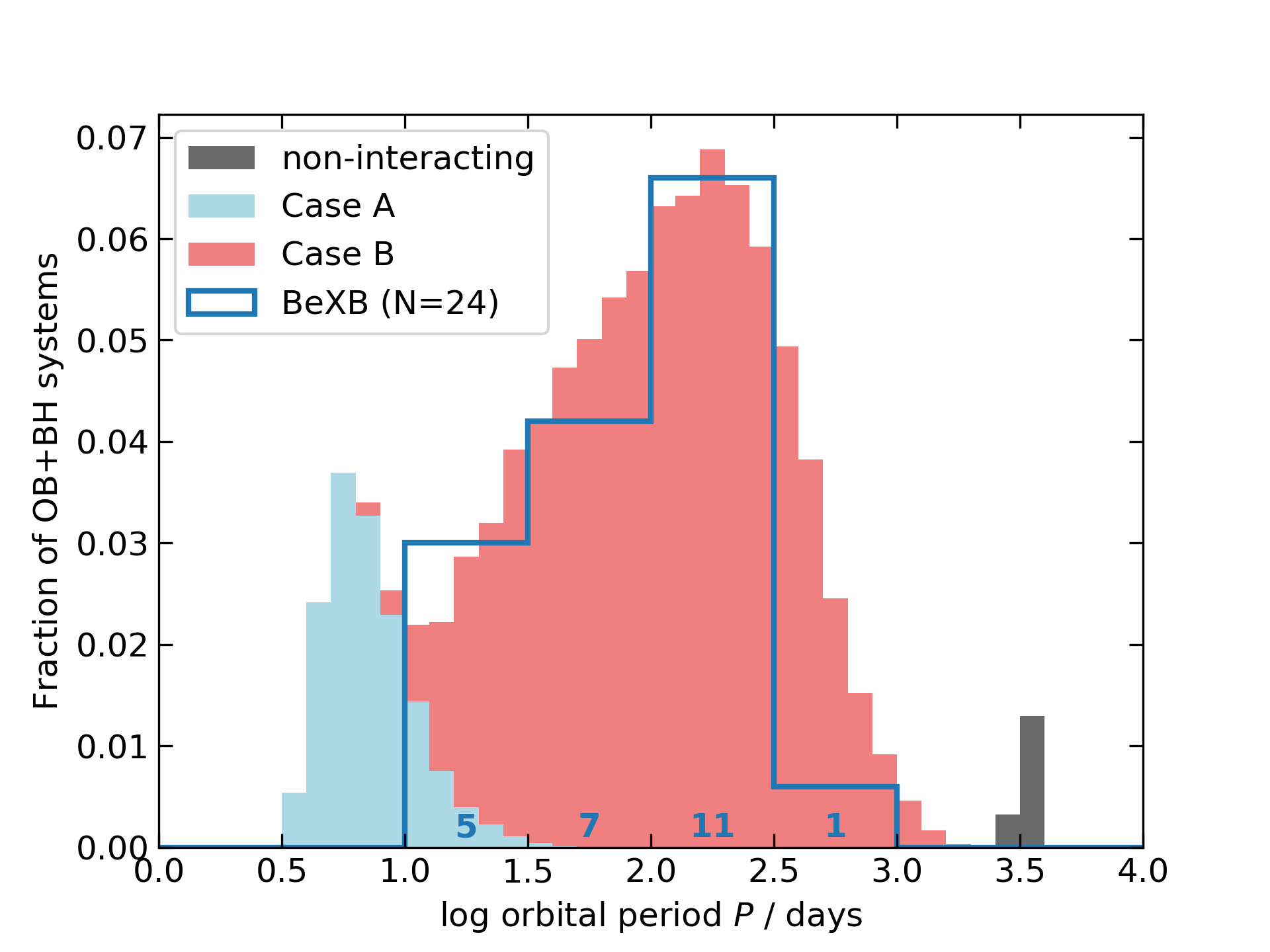
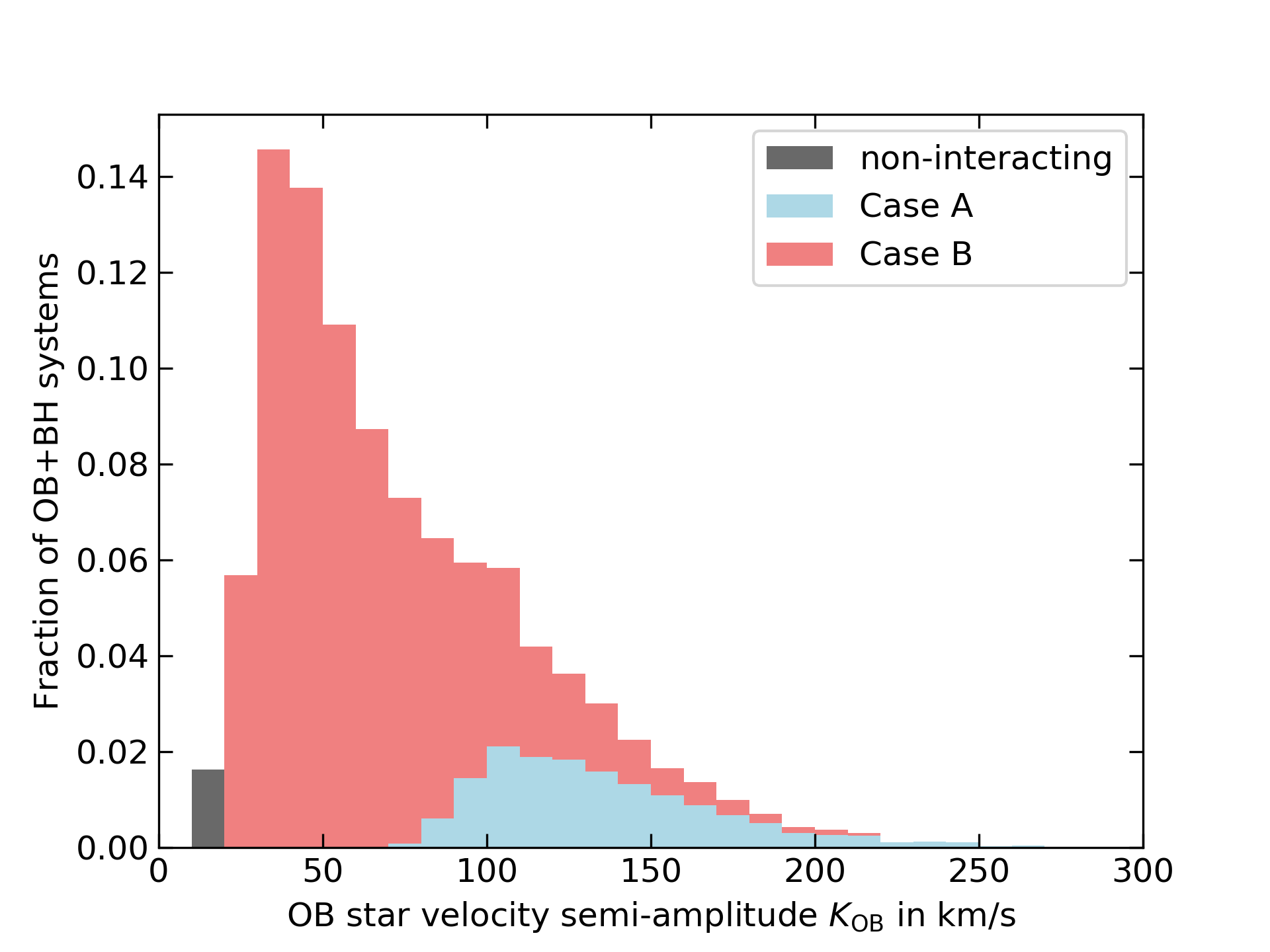
Figure 6: As Fig. 3, here showing the distribution of the orbital periods at the time of BH formation (top), and of the orbital velocity amplitudes (bottom) of our OB+BH binaries. The blue line in the top plot shows the distribution of the orbital periods of the Galactic Be/X-ray binaries (Walter et al. 2015).

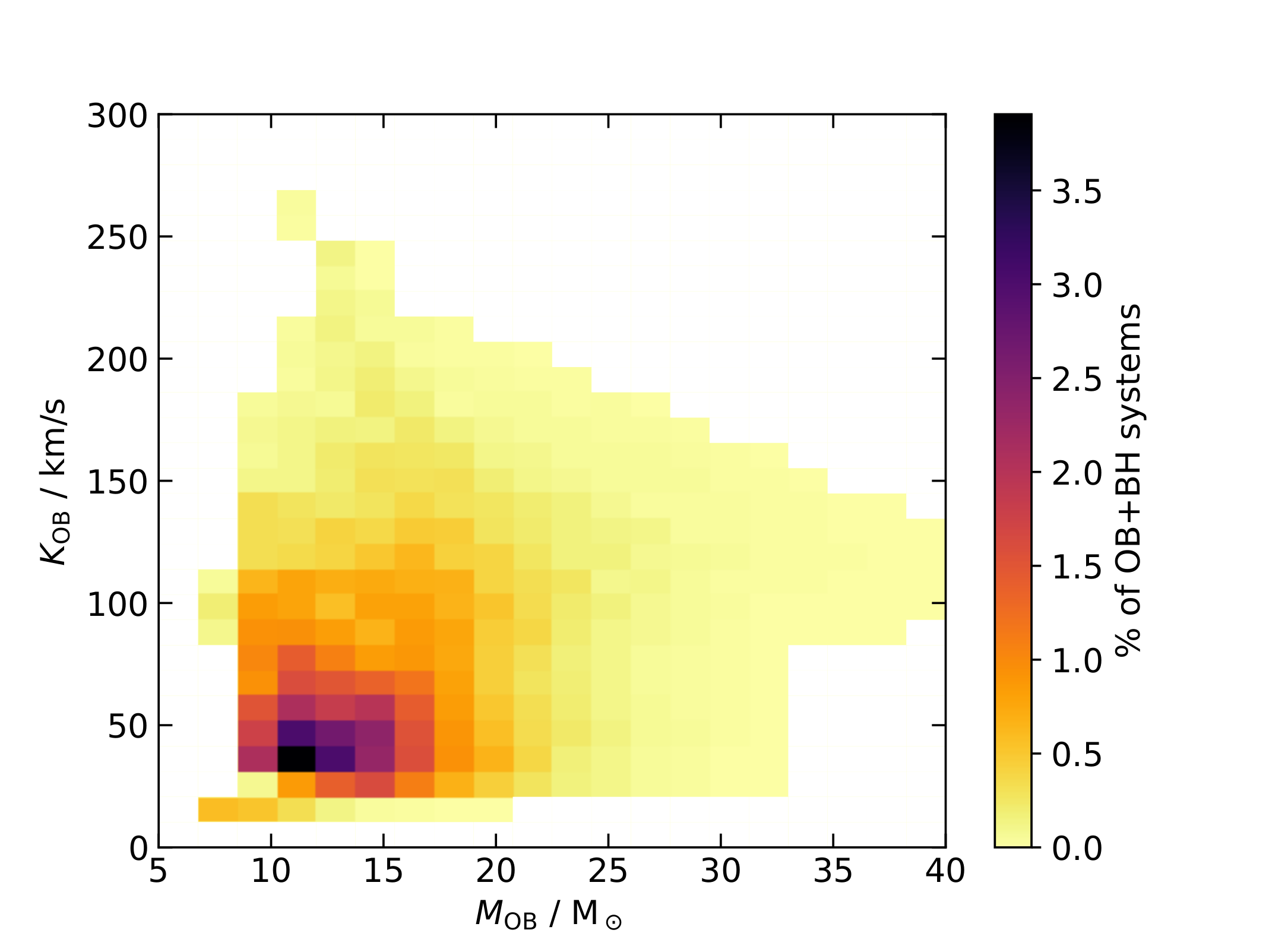
Figure 7: Predicted number distribution of OB+BH systems in the parameter space OB star mass$-$orbital velocity (top panel) and OB star mass$-$black hole mass (bottom panel). The expected numbers in each pixel are colour-coded and normalised such that the sum over all pixels is 100%.

The top panel of Fig. 6 shows the predicted distribution of orbital periods of the OB-BH binaries found in our model grid. We find that non-interacting binaries may produce OB+BH binaries with orbital periods in excess of about 3 yr. In Fig. 6 we can show only the shortest-period ones due to the upper initial period bound of our binary grid. Perhaps, many more such binaries may form, even small black hole formation kicks could break them up, the easier the larger the period. As these systems would also be the hardest to observed, we focus here on OB-BH binaries which emerge after mass transfer due to Roche-lobe overflow.

As seen in Fig. 6, the distribution of these post-interaction OB+BH binaries shows two distinct peaks, which we can attribute to the two distinguished modes of mass transfer. Not surprisingly, the Case A systems are found at smaller periods and remain below $\sim 30\,$d, while the Case B systems spread between about 10 d and 1000 d, with a pronounced maximum near 150 d. Overplotted in Fig. 6 is the observed orbital period distribution of 24 Galactic Be/X-ray binaries. We discuss the striking similarity with the period distribution of our OB+BH models in Sect. 6).

Through Kepler’s laws, we can convert the period distribution into a distribution of orbital velocities of the OB star components in OB+BH systems, which we show in the bottom panel of Fig. 6. As expected, the orbital velocities are largest in Case A binaries, and smallest in the Case B systems. These values are all so large that they are easily measurable spectroscopically (cf., Sect. 7).

Figure 7 illustrates the 2D-distributions of both component masses and the orbital velocity. In accordance with Fig. 3, we see that the OB masses are strongly concentrated to the mass range $8\,\mathrm{M}_{\odot}\dots 25\,\mathrm{M}_{\odot}$. The top figure shows that the OB+BH binaries are most abundant in a small area of the orbital velocity vs. OB mass plane, i.e., near $M_{\rm OB}\simeq 13\,\mathrm{M}_{\odot}$ and $K_{\rm OB}\simeq 50\,$km/s. More than half of all systems are expected to have OB masses below $17\,\mathrm{M}_{\odot}$ with orbital velocities of $K_{\rm OB}<70\,$km/s. At the same time, the bottom plot of Fig. 7 shows that the expected BH companions to $\simeq 13\,\mathrm{M}_{\odot}$ B stars have a rather flat distribution between $7\,\mathrm{M}_{\odot}$ and $20\,\mathrm{M}_{\odot}$ (see also Fig. 5).

3.3 OB star rotation and surface abundances

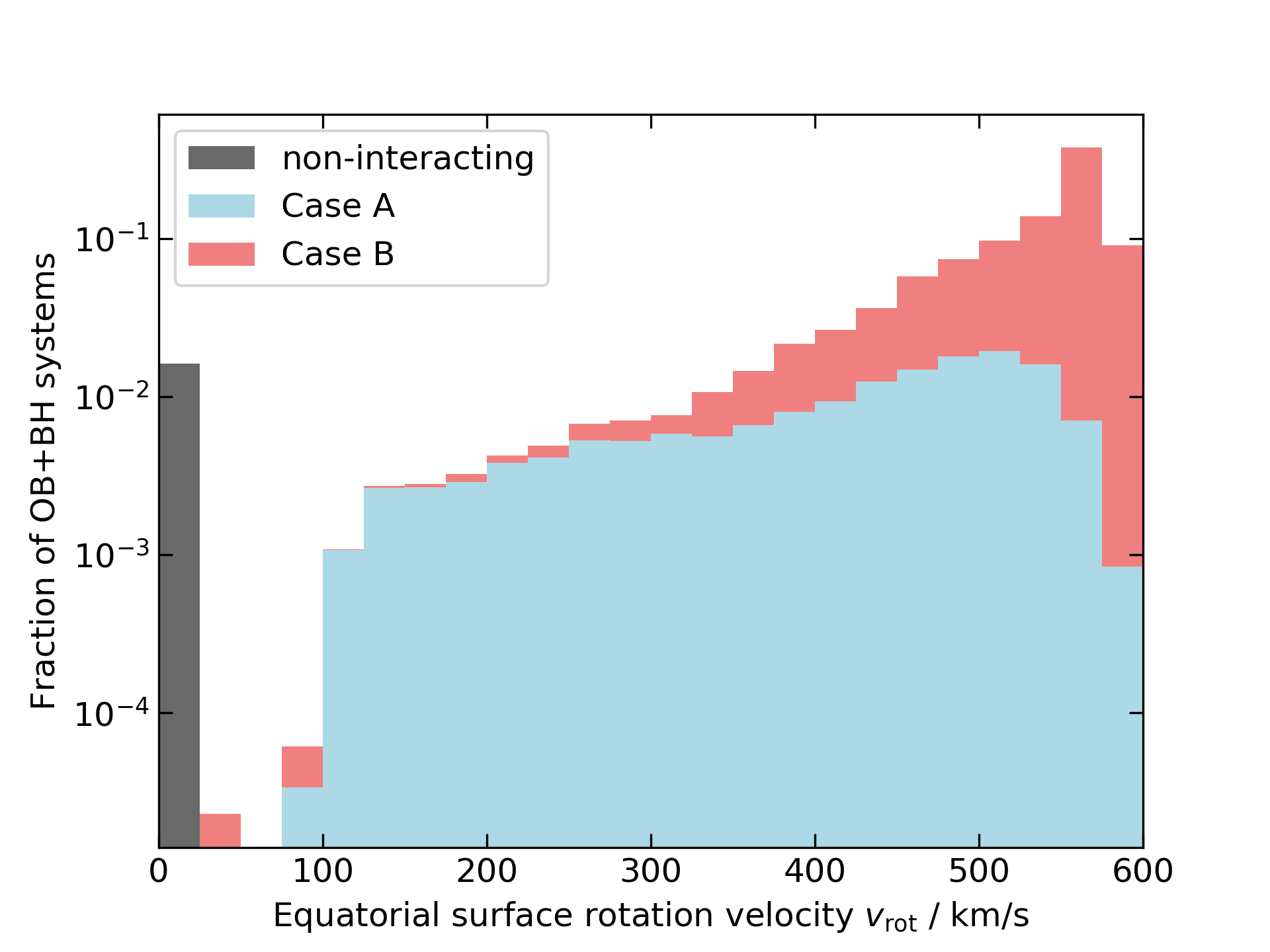
Figure 8: Distribution of the ratio of equatorial surface rotation velocity to critical rotation velocity for the OB stars in OB+BH binaries, at the moment of BH formation, as predicted by our population synthesis model (top panel). The bottom panel shows the corresponding distribution of the absolute equatorial surface rotation velocities of the OB stars as obtained in the indicated mass bins. In both plots, the small peak near zero rotation is due to the widest, non-interacting binaries; it is non-physical and should be disregarded.

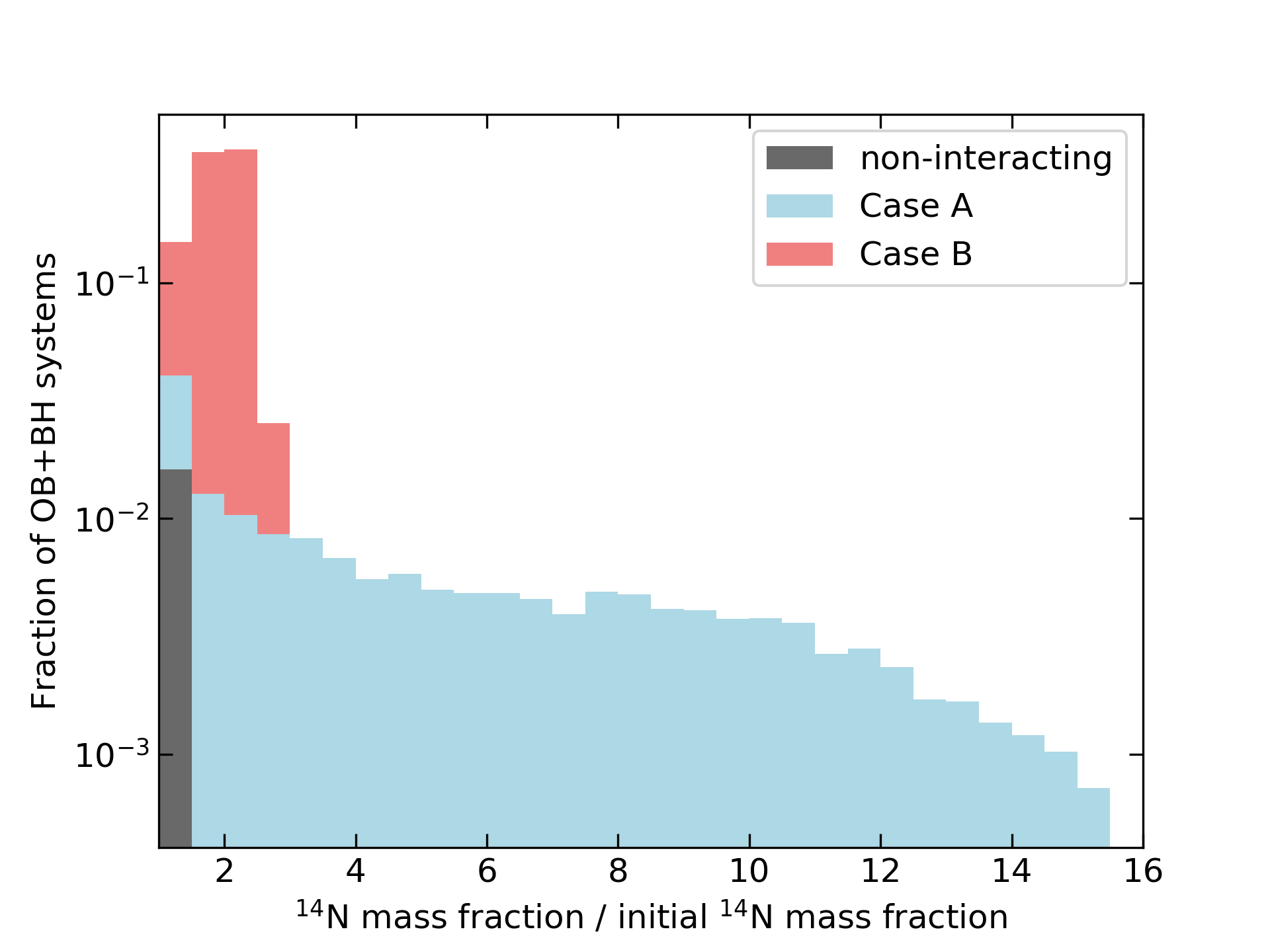
Figure 9: Result of our population synthesis calculations for the probability distribution of the surface helium (top) and nitrogen (bottom) surface abundances of the OB stars in OB+BH binaries.

As pointed out in Sect. 2, our detailed binary stellar evolution models accurately keep track of the angular momentum budget of both stars. They consider internal angular momentum transfer due to differential rotation, angular momentum loss by winds, angular momentum gain by accretion, and spin-orbit angular momentum exchange due to tides.

Figure 8 shows that most of the OB components in our OB+BH binary models are rapid rotators. At the time of BH formation, as many as half of them rotate very close to critical rotation. In particular, a high fraction of those systems which originate from Case B mass transfer, where tidal breaking is unimportant, rotate very close to critical. The Case A systems have a much broader distribution in Fig. 8. The minimum value of $\varv_{\rm rot}/\varv_{\rm crit}=0.2$ corresponds to the widest systems where tidal breaking still works, i.e., where the synchronisation timescale becomes comparable to the nuclear timescale of the OB star.

Looking at the absolute values of the rotational velocities, the bottom panel of Fig. 8 reveals a broader distribution. This is mostly an effect of the mass and time dependence of the critical rotational velocity. However, we see that even the Case A binaries stretch out to high rotation velocities, such that on average their rotation rate is much higher than that of an average O star (i.e., $\sim 150\,{\rm km}\,{\rm s}^{-1}$, Ramirez-Agudelo et al., 2013).

We point out that Fig. 8 depicts the rotation of the OB stars when the BH forms. In the time span between the end of the mass-transfer induced spin-up process and the BH formation, which corresponds to the core helium burning time of the BH progenitor in most cases, the OB star spin may have changed. The same is true for the lifetime of the OB star with a BH companion. Here, in particular the O stars are expected to lose some angular momentum due to their (non-magnetic) wind (Langer 1998, Renzo et al. 2017). On the other hand, single B stars are expected to spin-up as a consequence of their core hydrogen burning evolution (Ekstrom et al. 2008, Brott et al. 2011, Hastings et al. 2020). This explains that the B stars in our OB+BH binaries (i.e., the OB components with a mass below $\sim 15\,\mathrm{M}_{\odot}$), which are brought to critical rotation due to accretion, remain at critical rotation for their remaining hydrogen burning lifetime.

A second signature of accretion in the OB component of OB+BH binaries may be the presence of hydrogen burning products at the surface of the OB star. We note that in our models, rotationally induced mixing, semiconvection, and thermohaline mixing are included in detail. We find that the main enrichment effect is produced by the accretion of processed matter from the companion, and the subsequent dilution through thermohaline mixing. Despite the fast rotation of the OB components, rotational mixing plays no major role. The reason is that in contrast to rapidly rotating single star models, the spun-up mass gainers did not have an extreme rotation before the onset of mass transfer. During that stage, they could establish a steep H/He-gradient in their interior, which provides an unpenetrable barrier to rotational mixing after accretion and spin-up have happened.

To quantify the obtained enrichment, we show the distribution of the surface helium and nitrogen abundances of our OB stars with BHs in Fig. 9. We can see that the OB stars in Case B binaries remain essentially unenriched. The reason for this is that our Case B mass gainers accrete only small amounts of mass (about 10% of their initial mass). Furthermore, this accretion happens early during the mass transfer process, since the accretion efficiency drops once the stars are spun-up. Therefore, only material from the outer envelope of the donor star is accreted, which is generally not enriched in hydrogen burning products. We expect the near-critically rotating OB stars in our Case B systems to be Be stars. Given that Be stars are often not or only weakly enriched in nitrogen (Lennon et al. 2005, Dunstall et al. 2011), in contrast to predictions from rotating single star models, the population of Be stars may be dominated by binary-interaction products.

In Case A binaries, on the other hand, much more mass is accreted, also matter from the deeper layers of the mass donor, which have been part of the convective core in the earlier stages of hydrogen burning. As we see, the surface helium mass fraction goes up to $\sim 35$%. This is accompanied by a strong nitrogen enhancement by up to a factor of 12.

4 Key uncertainties

4.1 Envelope inflation

The largest considered initial primary mass in the LMC binary evolution model grid of Marchant (2016) is $39.8\,\mathrm{M}_{\odot}$. In a sense, this mass limit is an experimental result, since it was found that for the next higher initial primary mass to be considered ($44.7\,\mathrm{M}_{\odot}$), the MESA code could not compute through the mass transfer evolution of most systems. This is not surprising, since single star models computed with very similar physics assumptions (Brott et al. 2011) predict that such stars with LMC metallicity expand so strongly that they become red supergiants during core hydrogen burning. From an analysis of the internal structure of these models, Sanyal et al. (2015, 2017) found that this drastic expansion is a consequence of the corresponding models reaching the Eddington limit in their outer envelopes, when all opacity sources (i.e., not only electron scattering) are considered in the Eddington limit.

This so-called envelope inflation can be easily prevented to occur in stellar models. The corresponding envelope layers are convective, and an enhancement of the convective energy transport efficiency leads to a deflation of the envelope (fig. B.1 of Sanyal et al., 2015). However, there is no reason to doubt the energy transport efficiency of the classical Mixing Length Theory (Böhm-Vitense 1958) in this context. On the contrary, due to the low densities in the inflated envelope, it is evident that vertically moving convective eddies radiate away their heat surplus faster than they move, implying a small energy transport efficiency as computed by the standard Mixing Length Theory (Gräfener et al. 2012), which is also verified by corresponding 3D-hydrodynamic model calculations (Jiang et al. 2015). The inflation effect has been connected with observations of so-called Luminous Blue Variables (Gräfener et al. 2012, Sanyal et al. 2015, Grassitelli et al. 2020), which are hydrogen-rich stars; however, inflation is also predicted to occur in hydrogen-free stars (Ishii et al. 1999, Petrovic et al. 2006, Gräfener et al. 2012, Grassitelli et al. 2016).

Hydrogen-rich massive stars generally increase their luminosity and expand during their evolution. As a consequence, stars above a threshold mass reach the Eddington limit the earlier in their evolution the higher their mass (cf., fig. 5 of Sanyal et al. 2017). For the metallicity of the LMC, inflation occurs in stellar models above $\sim 40\,\mathrm{M}_{\odot}$ during late stages of hydrogen burning, and it occurs already at the zero age main sequence for masses above $\sim 100\,\mathrm{M}_{\odot}$. The implication for binary evolution above $\sim 40\,\mathrm{M}_{\odot}$ is that all models evolve into Case A mass transfer, i.e., Case B does not occur any more. Furthermore, the mass donors above $\sim 40\,\mathrm{M}_{\odot}$ have an inflated envelope at the onset of Roche-lobe overflow beyond a limiting initial orbital period which is smaller for higher donor mass. For hydrogen-free stars with a metallicity of the LMC, inflation occurs above a threshold mass of about $24\,\mathrm{M}_{\odot}$ (Ishii et al., 1999, Köhler et al. 2015, Ro 2019).

The inflated envelope of massive star models is fully convective (Sanyal et al. 2015). Furthermore, any mass loss increases the luminosity-to-mass ratio, thus increasing the Eddington factor. It is therefore not surprising that Quast et al. (2019) found the mass-radius exponent in such models to be negative (unless steep H/He-gradients are present in the outermost envelope). They showed that correspondingly, mass transfer due to Roche-lobe overflow is unstable, like in the case of red supergiant donors. In the absence of more detailed predictions, we therefore assume that mass transfer with an inflated mass donor leads to a common envelop evolution, and successively to the merging of both stars, in most cases.

In the mass-period diagram (Fig. 10), we have drawn the line beyond which a hydrogen-rich donor star (assuming here a hydrogen mass fraction of $X=0.4$) would exceed its Eddington limit. To construct this line, we have used the positions of single star models in the HR diagram in which inflation has increased the stellar radius by a factor of two, which coincides roughly (fig. 22 of Sanyal et al., 2015) with the hot edge of the LBV instability strip (Smith et al. 2004). For a given luminosity on this line, we obtained a corresponding stellar mass from the mass-luminosity relation of Gräfener et al. (2011) for a hydrogen mass fraction of $X=0.4$, and used the corresponding radius to obtain a binary orbital period for which stars on this line would fill their Roche-lobe radius for a mass ratio of 0.7. Considering that the orbital period change during Case A mass transfer is small (Qin et al. 2019), we would not expect to find WR+OB post-mass transfer binaries with H-rich WR stars above this line if binaries with significantly inflated donor stars would merge. For hydrogen-free Wolf-Rayet stars, the Eddingtion limit translates into a simple mass limit, which is also included in Fig. 10.

In Fig. 10, we plot the masses and orbital periods of the WN-type binaries in the LMC (Shenar et al. 2019). We note a group of five massive H-rich short-period WN+O binaries, for which it is unclear whether they did undergo mass transfer (cf., Shenar et al. 2019). In any case, they are indeed found below the Eddington limit, and are thus not in contradiction to having had mass transfer. The two very massive long-period binaries in Fig. 10, on the other hand, are clearly pre-interaction systems. Even though for lower hydrogen abundances, the line for the H-rich Eddington limit is expected to come down to lower masses, the two systems with WN masses just above 30$\,\mathrm{M}_{\odot}$ ($\log M_{\rm WN}\mathrel{\hbox{\hbox to0.0pt{\hbox{\lower 4.0pt\hbox{$\sim$}}\hss}\hbox{$>$}}}1.5$) show a hydrogen mass fraction of $\sim 0.2$ in the WN star, for which they would still not violate the Eddington limit. Furthermore, we see that all hydrogen-free WN stars are located below the corresponding horizontal line. We conclude that the properties of the LMC WN binaries are in agreement with the assumption that inflated donors lead to mergers.

Since H-free Wolf-Rayet stars may be very close to collapsing to a BH, we add the massive black hole binaries to Fig. 10 for which the black hole mass is well constrained. Note that we do not include the low- and intermediate mass black hole binaries here (cf., Casares & Jonker 2014); their progenitor evolution is not well understood (Wang et al., 2016). Figure 10 shows that the massive black hole binaries occupy a similar parameter space as the hydrogen-free WN stars. Figure 10 can not resolve whether binaries with initial primary masses above 40$\,\mathrm{M}_{\odot}$ contribute to the massive BH-binary population. However, the properties of M33-X7 argue for such a contribution, since in this binary the BH companion is an O star of $\sim 70\,\mathrm{M}_{\odot}$. This is not in conflict with the Eddington limit due to the short orbital period, which implies a progenitor evolution via Case A mass transfer (Valsecchi et al. 2010, Qin et al. 2019).

Nevertheless, Fig. 10 suggests that the contribution of stars above 40$\,\mathrm{M}_{\odot}$ to the population of massive BH-binaries is mostly constrained to orbital periods below $\sim 10\,$d. Therefore, we can consider the predictions for the number of OB+BH binaries from our Case A binary evolution models as a lower limit, and the corresponding OB star mass distribution for Case A (Fig. 3) to stretch out to higher OB masses. Our predictions for larger period OB+BH binaries, which are mostly due to Case B evolution, might not be affected much by this uncertainty.

4.2 Mass transfer efficiency

Observations of massive post-mass transfer binaries suggest that the mass transfer efficiency, i.e., the ratio of the amount of mass accreted by the mass gainer to the amount of mass lost by the mass donor due to Roche-lobe overflow, is not the same in different binaries. Whereas some can be better understood with a high mass transfer efficiency, others require highly non-conservative mass transfer (e.g., Wellstein & Langer 1999, Langer et al. 2003). Petrovic et al. (2005) argue for lower efficiency in systems with more extreme mass ratios, and de Mink et al. (2007) derive evidence for a lower efficiency in wider binary systems.

Our mass transfer model (cf., Sect. 2), which assumes that the mass transfer efficiency drops when the mass gainer is spinning rapidly, does in principle account for these variations. However, it requires that sufficient mass is removed from the binary to prevent the mass gainer from exceeding critical rotation. We apply the condition that the photon energy emitted by the stars in a binary is larger than the gravitational energy needed to remove the excess material. Otherwise, we stop the model and assume the binary to merge. Figure 2 shows the dividing line between the surviving and merging for our models with an initial primary mass of 25.12$\,\mathrm{M}_{\odot}$. The predicted number of OB+BH binaries is roughly proportional to the area of surviving binaries in this figure.

This condition for distinguishing stable mass transfer from mergers is rudimentary and will need to be replaced by a physical model eventually. Correspondingly uncertain is the number of predicted OB+BH binaries. However, Wang et al. (2020) have shown that the distribution of the sizable Be population of NGC 330 (Milone et al. 2018) in the colour-magnitude diagram is well reproduced by detailed binary evolution models. In order to explain their number, however, the condition for stable mass transfer would have to be relaxed such that merging is prevented in more systems. A corresponding measure would increase the predicted number of OB+BH binaries, such that, again, our current numbers could be considered as a lower limit.

4.3 Black hole formation

As discussed in Sect. 2, our BH formation model is very simple. By applying the single star helium core mass limit according to simple criteria based on one-dimensional pre-collapse models, and by neglecting small mass ranges above that limit which may lead to neutron stars rather than black holes, we may overpredict the number of OB+BH systems. However, the anticipated BH mass distribution is rather flat (Fig. 5), such that this overprediction is likely rather small. Our assumption that the black hole mass equals the final helium core mass is perhaps not very critical, since it does not affect the predicted number of OB+BH systems.

The neglect of a BH birth kick may again lead to an overprediction of OB+BH binaries. However, due to the much larger mass of the BHs compared to neutron stars, birth kicks with similar momenta as those given to neutron stars upon their formation would still leave most of the OB+BH binaries intact. While Janka (2013) suggests that NS and BH kick velocities can be comparable in BHs which are produced by asymmetric fallback, Chan et al. (2018) find only modest BH kicks in their simulations. By considering the galactic distribution of low-mass BH binaries, Repetto & Nelemans (2015) find 2 out of 7 systems were consisted with a relatively high BH formation kick. This result is confirmed by Repetto et al. (2017), who find, on the other hand, that the galactic scale hight of the low mass BH binaries is smaller than that of the low mass NS binaries. Mirabel (2017) provides evidence for the BHs of $\sim 10\,\mathrm{M}_{\odot}$ and $\sim 15\,\mathrm{M}_{\odot}$ in the high mass black hole binaries GRS 1915+105 and Cygnus X-1 formed with essentially no kick. Furthermore, the systems which may correspond closest to the our predicted OB+BH distribution, the galactic Be+BH binary MCW 656 (Casares et al. 2014) and the potential B+BH binary LB1 (Liu et al. 2019; see our discussion on this in Sect. 6), appear to have low eccentricities. We consider the systematics of BH kicks to be still open and return to a discussion of their effect on OB+BH systems in Sect. 5.

5 Comparison with earlier work

The computation of large and dense grids of binary evolution models has so far been performed mostly by using so-called rapid binary evolution codes (e..g., Hurley et al. 2002, Voss & Tauris 2003, Izzard et al 2004, Vanbeveren et al. 2012 , de Mink et al. 2013, Lipunov & Pruzhinskaya 2014, Stevenson et al 2017, Kruckow et al. 2018). On the one hand, such calculations can comprehensively cover the initial binary parameter space, and they allow an efficient exploration of uncertain physics ingredients. On the other hand, stars are spatially resolved by only two grid points, binary interaction products are often described by interpolating in single star models. Therefore, many genuine binary evolution effects are difficult to include, which is true for the uncertainties discussed in Sect. 4.

The computation of dense grids of detailed binary evolution models has become feasible in the last decade or so (Nelson & Eggleton 2001, de Mink et al. 2007, Eldridge et al. 2008, Eldridge & Stanway 2016, Marchant et al. 2016, 2017; see also van Bever & Vanbeveren 1997). Whereas the computational effort is much larger, detailed calculations are preferable over rapid binary evolution calculations whenever feasible. Detailed binary model grids have been used to explore various stages and effects of binary evolution, including the production of runaway stars (Eldridge et al. 2011), double black hole mergers (Eldridge & Stanway 2016, Marchant et al. 2016) long-duration gamma-ray bursts (Chrimes et al. 2020), ultraluminous X-ray sources (Marchant et al. 2017), and galaxy spectra (Stanway & Eldridge 2019). However, a detailed prediction of the OB+BH binary population has not yet been performed.

Many rapid binary evolution calculations exist. Here, papers predicting OB+BH populations often aim at reproducing the observed X-ray binary populations (e.g., Dalton & Sarazin 1995, Tauris & van den Heuvel 2006, Van Bever & Vanbeveren 2000, Andrews et al. 2018). For example, based on the apparent lack of B+BH binaries in the population of the Galactic X-ray binaries, Belczynski & Ziolkowski (2009) predicted a very small number of such systems, using rapid binary evolution models. Since the discovery of the massive black hole mergers through gravitational waves, many predictions for the expected number of double compact mergers have been computed based on rapid binary evolution models (e.g., Chruslinska et al. 2018, Kruckow et al. 2018, Vigna-Gomez et al. 2018, Spera et al. 2019). However, whereas the binary evolution considered in these papers includes the OB+compact object stage, their predictions are focused on the double compact mergers.

In the last few years, based on an analytic considerations, Mashian & Loeb (2017), Breivik et al. (2017), Yamaguchi et al. (2018), Yalinewich et al. (2018) and Masuda & Hotokezaka (2019) developed predictions for the BH-binary population in the Galaxy. Much of this work concentrates on low-mass MS+BH binaries, in view of the currently known 17 low-mass black hole X-ray binaries (McClintock & Remillard 2006, Arur & Maccarone 2018). Shao & Li (2019) have recently simulated the Galactic BH-binary population through rapid binary evolution models, with detailed predictions for OB+BH binaries. As they are largely consistent with the outcome of the quoted earlier papers, we compare our results with theirs.

As shown in Sect.6, our results imply that the LMC should currently contain about 120 OB+BH binaries. Assuming a ten times higher star-formation rate in the Milky Way (Diehl et al. 2006, Robitaille & Whitney 2010) would lead to 1200 Galactic OB+BH binaries. Here we neglect the metallicity difference between both systems, which, indeed, for stars below $40\,\mathrm{M}_{\odot}$, is not expected to cause big differences (e.g., Brott et al. 2011), at the level of the accuracy of our consideration. Shao & Li exploit the advantage of rapid binary calculations by producing four population models for Galactic MS+BH binaries, which differ in the assumptions made for the BH kick distribution (see also Renzo et al. 2019). They find that essentially no low-mass BH-binaries are produced if efficient BH kicks are assumed. Given the observed number of low-mass black hole X-ray binaries, Shao & Li discard the possibility of efficient BH kicks. For the other cases, they predict between 4 000 and 12 000 Galactic OB+BH binaries. This number exceeds our estimate for the number of Galactic OB+BH binaries by a factor of 3 to 10.

We find three potential reasons for this. First, Shao & Li adopt a very small accretion efficiency. As in our detailed models, they assume that the spin-up of the mass gainer limits the mass accretion. However, in our models, we check whether the energy in the radiation field of both stars is sufficient to remove the excess material from the binary system is sufficient, and assume the binary merges if not. No such check is applied by Shao & Li, with the consequence that binaries with initial mass ratios as small as 0.17 undergo stable mass transfer. Comparing this with our Fig. 2 shows that this might easily lead to a factor of two more OB+BH binaries. Furthermore, Shao & Li assume that BH can form from stripped progenitors with masses above 5$\,\mathrm{M}_{\odot}$ (we adopted a limit of 6.8$\,\mathrm{M}_{\odot}$; see Sect. 2), and do not discard progenitors with initial primary masses above 40$\,\mathrm{M}_{\odot}$ as envelope inflation (see Sect. 4) is not considered in their models. While both effects lead to more OB+BH binaries, they may not be as important as the first one.

The distribution of the properties of the OB+BH binaries found by Shao & Li is similar to those predicted by our models. The OB stars show a peak in their mass distribution near 10$\,\mathrm{M}_{\odot}$, and the BH masses fall in the range 5$\dots$15$\,\mathrm{M}_{\odot}$ with a peak near 8$\,\mathrm{M}_{\odot}$. The orbital periods span from 1 to 1000 days, with a peak near $\sim$100 days, and is similar to that found by Shao & Li (2014) for Be+BH binaries. Naturally, the peak produced by our Case A systems (Fig. 6) is not reproduced by the rapid binary evolution models.

6 Comparison with observations

The global H$\alpha$-derived star formation rate of the LMC is about $\sim 0.2\,\,\mathrm{M}_{\odot}\leavevmode\nobreak\ {\rm yr}^{-1}$ (Harris & Zaritsky, 2009). About a quarter of that is associated with the Tarantula region, for which the number of O stars is approximately 570 (Doran et al., 2013, Crother 2019). We therefore expect about 2000 O stars to be present in the LMC. About 370 of them have been in the spectroscopic VLT Flames Tarantula survey (Evans et al. 2011). Adopting a 3% probability for a BH companion as suggested by our results (cf., Sect. 7), we expect about 60 O+BH binaries currently in the LMC. About 10 of them may have been picked up by the Tarantula Massive Binary Monitoring survey (Almeida et al. 2017).

At the same time, we also predict about 1.5% of the B stars above $\sim 10\,\mathrm{M}_{\odot}$ to have a BH companion, most of which would likely be Be stars. As they live roughly twice as long as O stars, and accounting for a Salpeter mass function, we expect about 60 B+BH binaries amongst the $\sim 4000$ B stars above $10\,\mathrm{M}_{\odot}$ expected in the LMC. This means that our models predict more than 100 OB+BH systems in the LMC, while we know only LMC-X1. The implication is either that our model predictions are off by some two orders of magnitude, or that the majority of OB+BH binaries are X-ray quiet.

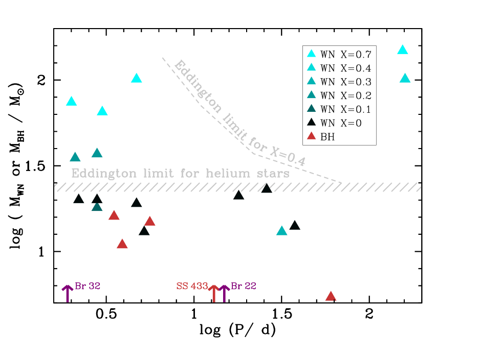
Figure 10: Masses and orbital periods of LMC WN binaries with an O or early B star companion (Shenar et al. 2019). The orbital periods of the two LMC WC binaries Br 22 (right) and Br 32 (left; Boisvert et al. 2008) and of SS 433 (Hillwig & Gies 2008) are indicated by arrows. Also plotted are the masses and orbital periods of the well characterised black holes with O or early B companion, which are, in order of increasing orbital period, M33-X7 (Orosz et al. 2007), LMC-X1 (Orosz et al. 2011), Cyg-X1 (Orosz et al. 2011), and MCW 656 (Casares et al. 2014). Above $\sim 24\,\mathrm{M}_{\odot}$ (or a corresponding luminosity of $\log\,L/{\rm L}_{\odot}\,=5.8$; Gräfener et al. 2011), no H-free Wolf-Rayet stars are known in the LMC, potentially because this corresponds to their Eddington limit (see text).

One way to decide which of these two answers is right is to consider the Wolf-Rayet binaries in the LMC. Shenar et al. (2019) have provided the properties of 31 known or suspected WN-type LMC binaries. Of those, an orbital period is known for 16, which we show in Fig. 10. Of these 16 WN binaries, seven are hydrogen-rich (with hydrogen mass fractions in the range $0.7\dots 0.2$), very massive, and likely still undergoing core hydrogen burning. The other nine are very hot, and most of them hydrogen-free, such that they are likely undergoing core helium burning. As this implies a short remaining lifetime, they are likely close to core collapse. In fact, taking their measured mass-loss rates and adopting an average remaining Wolf-Rayet lifetime of 250 000 yr would leave most of them at the end of their lives well above $10\,\mathrm{M}_{\odot}$. We can thus assume here that these nine OB+WN binaries will form OB+BH systems. Once the Wolf-Rayet stars forms a BH, the OB stars will on average still live for a long time. A remaining OB star lifetime of 1 or 2 Myr leads to the expectation of 18$\dots$36 OB+BH binaries currently in the LMC, which is rather close to our model prediction. About 16% of the 154 Wolf-Rayet stars in the LMC are of type WC or WO (Breysacher et al. 1999, Neugent et al. 2018). Their properties are less well known; however, at least three of the 24 WC stars are binaries (the two with well determined orbital period are included in Fig. 10). Including the WC binaries will increase the expected number of OB+BH binaries (Sander et al. 2019).

When we look at the properties of the observed WR+OB binaries, we find that the OB star masses in the mentioned nine binaries ($13\dots 44\,\mathrm{M}_{\odot}$) are well within the range predicted by our models (Fig. 3). However, the average observed OB mass of the nine WR+OB binaries is $\sim 26\,\mathrm{M}_{\odot}$, while the average OB mass of our OB+BH models is about $15\,\mathrm{M}_{\odot}$ (Fig. 3). In fact, amongst the nine considered LMC systems, only one has a B dwarf component (Bat 29). Of the other potential WR-binaries listed by Shenar et al. (2019), one more has a B dwarf companion but no measured orbital period, and three more apparently have rather faint B supergiant companions (which is difficult to understand in evolutionary terms). We note that our models predict that the B stars in such binaries could be rapidly rotating, and that it is unclear whether a Be disk can be present next to a WR star with a powerful wind. Potentially, the spectral appearance of B stars in this situation may be unusual. Furthermore, O dwarfs are perhaps easier identified as WR star companions than the fainter B dwarfs, such that more of the latter could still be discovered. Another aspect to consider is that a considerable fraction of the He-star companions of B dwarfs might not have a WR-type spectral appearance. Their luminosity-to-mass ratio might simply be too low to yield a sufficient mass-loss for an emission-line spectrum (Sander et al. 2020, Shenar et al. 2020), eliminating them from being found in WR surveys

Concerning the orbital periods, a comparison of Fig. 6 with Fig. 10 shows that five of the nine considered WN+OB binaries are found in the period range predicted by our Case A binary models, whereas the other four fall into the Case B regime. Notably, the gap in the observed periods ($7\dots 15\,$d) coincides with the minimum in the predicted period distribution produced between the Case A and Case B peaks in the top panel of Fig. 6. On the other hand, our Case B models predict a broad distribution of orbital periods with a peak near 100 d, whereas the largest measured period is 38 d (Bat 64). Again, this could mean two things. Either our models largely overpredict long-period OB+WN binaries (with core helium burning WN stars), or many long-period systems have not yet been identified. In this respect, we note that Shenar et al. (2019) list nine more binaries in which the WR star is likely undergoing core helium burning but for which no period has been determined. Since longer periods are harder to measure, there could be a bias against finding long period systems.

This idea is fostered by considering the Be/X-ray binaries. This may be meaningful as their evolutionary stage is directly comparable to the OB+BH stage, only that the primary star collapsed into a NS, rather than a BH. Because of the larger mass loss and the expected larger kick during neutron star formation, in particular the longest period OB+NS systems may break-up at this stage, whereas comparable OB+BH systems might survive. However, otherwise, we would expect their properties to be quite similar to those of OB+BH systems. The orbital period distribution of the Galactic Be/X-ray binaries is quite flat and stretches between 10 d and 500 d (Reig 2011, Knigge et al. 2011, Walter et al. 2015). Overplotted in Fig. 6 is the observed orbital period distribution of 24 Galactic Be/X-ray binaries following Walter et al. Figure 6 shows that the orbital period distribution of the Be/X-ray binaries matches the prediction of our Case B OB+BH binaries very closely. Since the pre-collapse binary evolution does not know about whether a NS or BH will be produced by the mass donor, the observed Be/X-ray binary period distribution argues for the existence of long-period OB+BH binaries as predicted by our models.

Looking at the location of the four massive black hole binaries in the mass-orbital period plot in comparison to the OB+WR binaries in Fig. 10, we find that three of them coincide well with the short-period helium burning WR binaries within the Case A range of our models (see also Qin et al., 2019). Only the Be-BH binary MCW 656 has a rather large orbital period of 60 d. Our conjecture of the existence of many more long-period OB+BH binaries agrees with the anticipation of Casares et al. (2014), who consider MCW 656 only as the tip of the iceberg. The reason is that MCW 656, in contrast to the short-period OB+BH systems, is X-ray silent, which is likely due to the fact that the wind material falling onto the BH does not form an accretion disk but an advection-dominated inflow (Shakura & Sunyaev 1973, Karpov & Lipunov 2001, Narayan & McClintock 2008, Quast & Langer 2020). We note that also the recently detected B star$-$BH binary system LB-1 (Liu et al. 2019) might fall into this class. While it was first proposed that the BH in this system is very massive, it has been shown subsequently that its mass is consistent with being quite ordinary (Abdul-Masih et al. 2019b, El-Badry & Quataert 2020, Simon-Dias et al. 2020), if it is a BH at all (Irrgang et al. 2020).

Remarkably, it is the long-period OB+BH binaries which have the highest chance to produce a double-compact binary which may merge within one Hubble time.

7 OB+BH binary detection strategies

We have seen above that our binary evolution models predict that about 100 OB+BH binaries remain to be discovered in the LMC. Scaling this with the respective star-formation rates would lead to something like 500 to several thousand OB+BH binaries in the MW. Simplified binary population synthesis models predict similar numbers, and show that the order of magnitude of the expected number of OB+BH binaries is only weakly dependent on the major uncertainties in the models (Yamaguchi et al. 2018, Yalinewich et al. 2018, Shao & Li 2019). At the same time, as discussed in Sect. 6, the observations of Wolf-Rayet binaries and of Be/X-ray binaries, lend strong support to these numbers. Finding these OB+BH binaries, and measuring their properties, would provide invaluable boundary conditions for the evolution and explosions of massive stars.

One possibility is to monitor the sky position of OB stars and determine the presence of dark companions from detecting periodic astrometric variations. It has been demonstrated recently that the Gaia satellite offers excellent prospects for identifying OB+BH binaries this way (Breivik et al. 2017; Mashian & Loeb 2017; Yalinewich et al. 2018; Yamaguchi et al. 2018, Andrews et al. 2019). Furthermore, a BH companion induces a photometric variability to an OB star in several ways (Zucker, et al. 2007, Masuda & Hotokezaka 2019). In the closest OB+BH binaries, the OB star will be deformed which leads to ellipsoidal variability. In wide binaries seen edge-on, gravitational lensing of the BH can lead to significant signals (App. A). Additionally, relativistic beaming due to the orbital motion affects the light curve of OB+BH binaries. Masuda & Hotokezaka find that the TESS satellite may help to identify OB+BH binaries, in particular short-period ones. Finally, OB+BH binaries can be identified spectroscopically, through the periodic radial velocity shift of the OB component in so-called SB1 systems, in which only one star contributes to the optical signal. Spectacular examples are provided by the discovery of the first known Be-BH binary (Casares et al. 2014), the potentially similar B[e]-BH binary candidate found by Khokhlov et al. (2018) and the recently found potential B-BH binary LB-1 (Liu et al 2019; see Sect. 6). Existing surveys include the TMBM survey in the LMC (Almeida et al., 2017), and the Galactic LAMOST survey (Yi et al. 2019).

Whichever way the BHs in binary systems affect the signal we are observing from the companion star, the BH per se will remain unobservable. This means that the conclusion of having a BH in a given binary will always remain indirect, and — as physics can never deliver proofs — somewhat tentative. This is the more so as, obviously, the technique with which BH detections are generally associated, namely X-ray observations, appears to fail for the vast majority of OB+BH binaries (cf., Sect. 6). For that reason, it will be beneficial if, firstly, OB+BH binaries are detected in more than one ways, and secondly, if the properties of the OB component are measured spectroscopically, to see whether e.g. its surface abundances and its rotation rate fall within expectations.

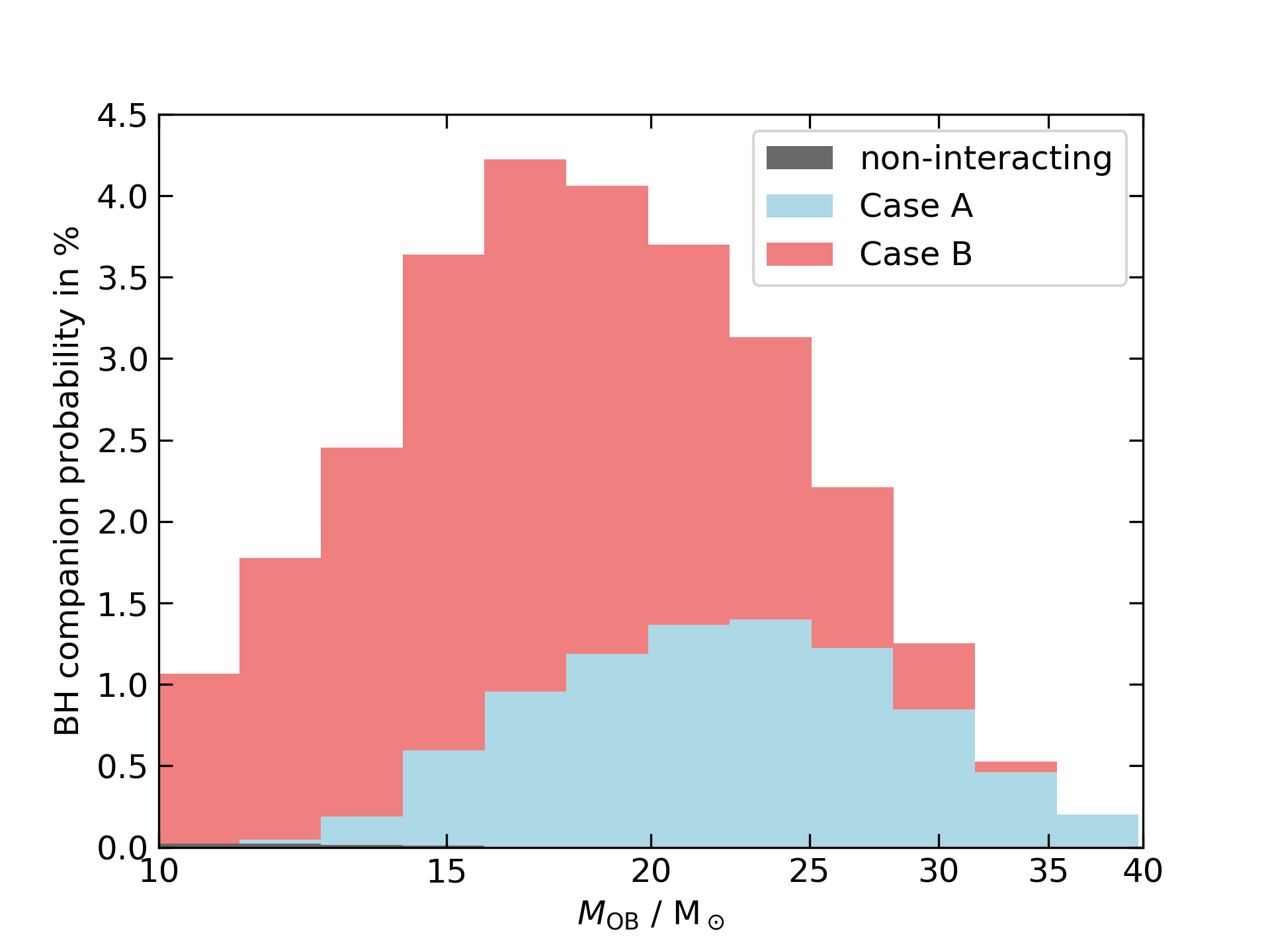
Figure 11: Probability of OB stars of a given mass to have a BH companion, as function of the mass of the OB star, according to our population synthesis model. The initial mass function, initial binary parameter distributions, and the lifetimes of the OB+BH systems have been considered. A initial binary fraction of 100% has been assumed.

In our grid of binary evolution models, we produce (potential) OB+BH binaries, but the model systems spend their largest amount of time as OB+OB binaries. In order to evaluate the probability that a randomly picked OB star has a BH companion, we divide the number of systems in the mass bin of our OB star to the corresponding number of OB binaries with any type of companion. The result is plotted in Fig. 11. Here, OB single stars are neglected. Considering them does reduce the probabilities obtained in Fig. 11 by the assumed binary fraction.

Figure 11 resembles the overall OB star mass distribution derived in Fig. 3. However, its ordinate values represent actual BH companion probabilities. Therefore, we find that the fraction of OB stars with BH companions is highest in the OB star mass range $14\dots 22\,\mathrm{M}_{\odot}$, with the probability to have an accompanying BH of about 4%. For B stars near $10\,\mathrm{M}_{\odot}$, the BH companion probability is still about 1%. For more massive OB stars, we expect BH companions in at least 1% of the stars up to about 32$\,\mathrm{M}_{\odot}$, where an additional contribution from binaries with initial primary masses above $40\,\mathrm{M}_{\odot}$ is possible (see Sect. 4).

In the upper panel of Fig. 12, we show the probability of a randomly picked OB binary to have a BH companion, as function of its orbital period. For example, if our chosen binary has an orbital period of 10 d, then its chance to be accompanied by a BH is about 1.5%. For a period of 180 d, on the other hand, it is almost 8%. Figure 12 shows that the expected orbital periods in OB+BH binaries are somewhat ordered according to their initial orbital periods. The Case A systems have the smallest initial periods (cf., Fig. 2), and they produce the shortest period OB+BH binaries in our results. On the opposite side, the initial period range of the Case B binaries is mapped into a quite similar period range of the OB+BH binaries.

The lower panel of Fig. 12 shows the corresponding distribution of orbital velocities. Again, the ordinate value in this plot reflects the probability of a randomly picked OB binary to contain a BH, this time as function of its orbital velocity. The Case A systems, which have initial orbital periods as low as 1.4 d, provide the fastest moving OB stars, while the Case B binaries form many OB+BH systems with orbital velocities of just a few tens of km/s.

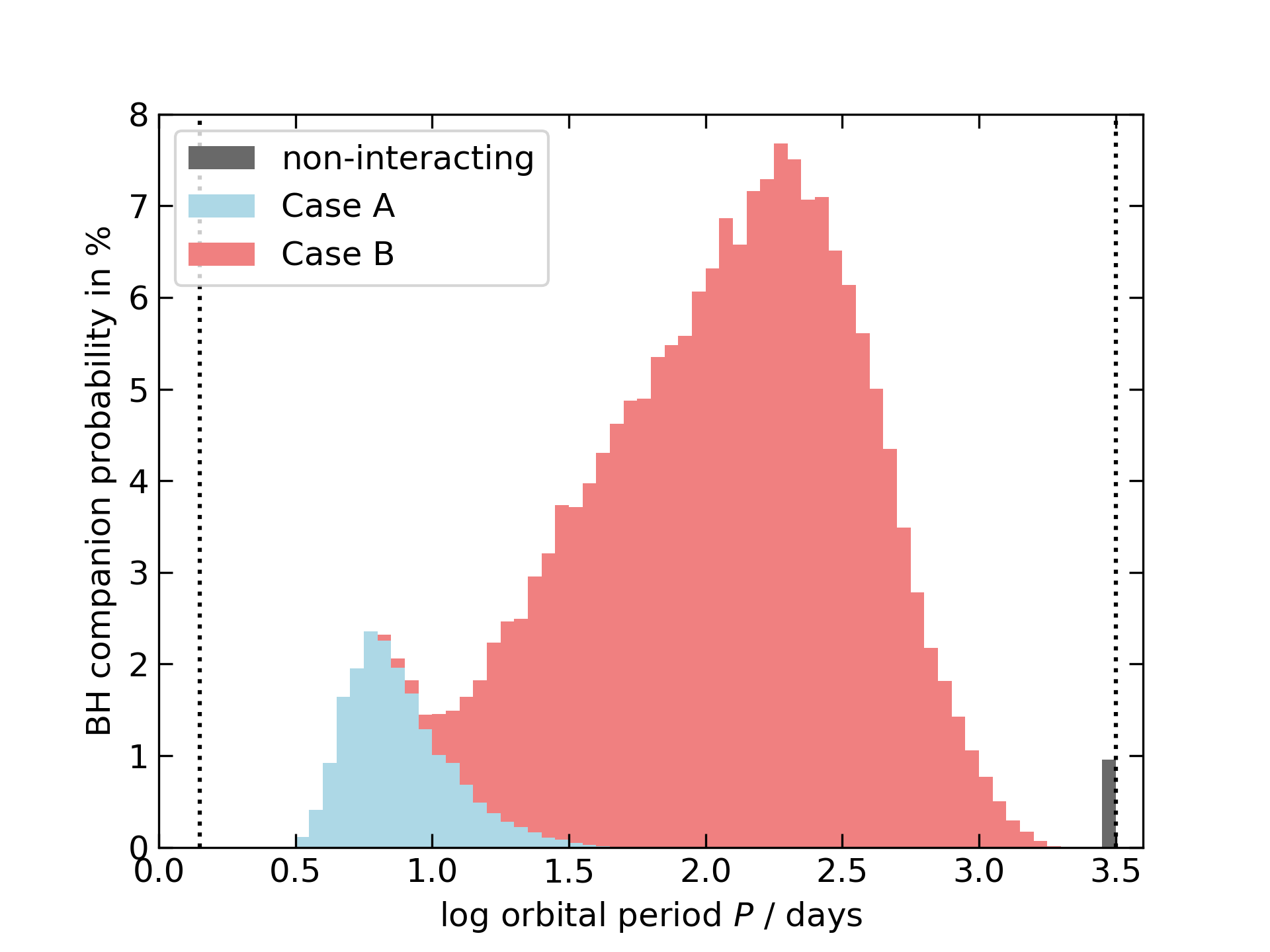
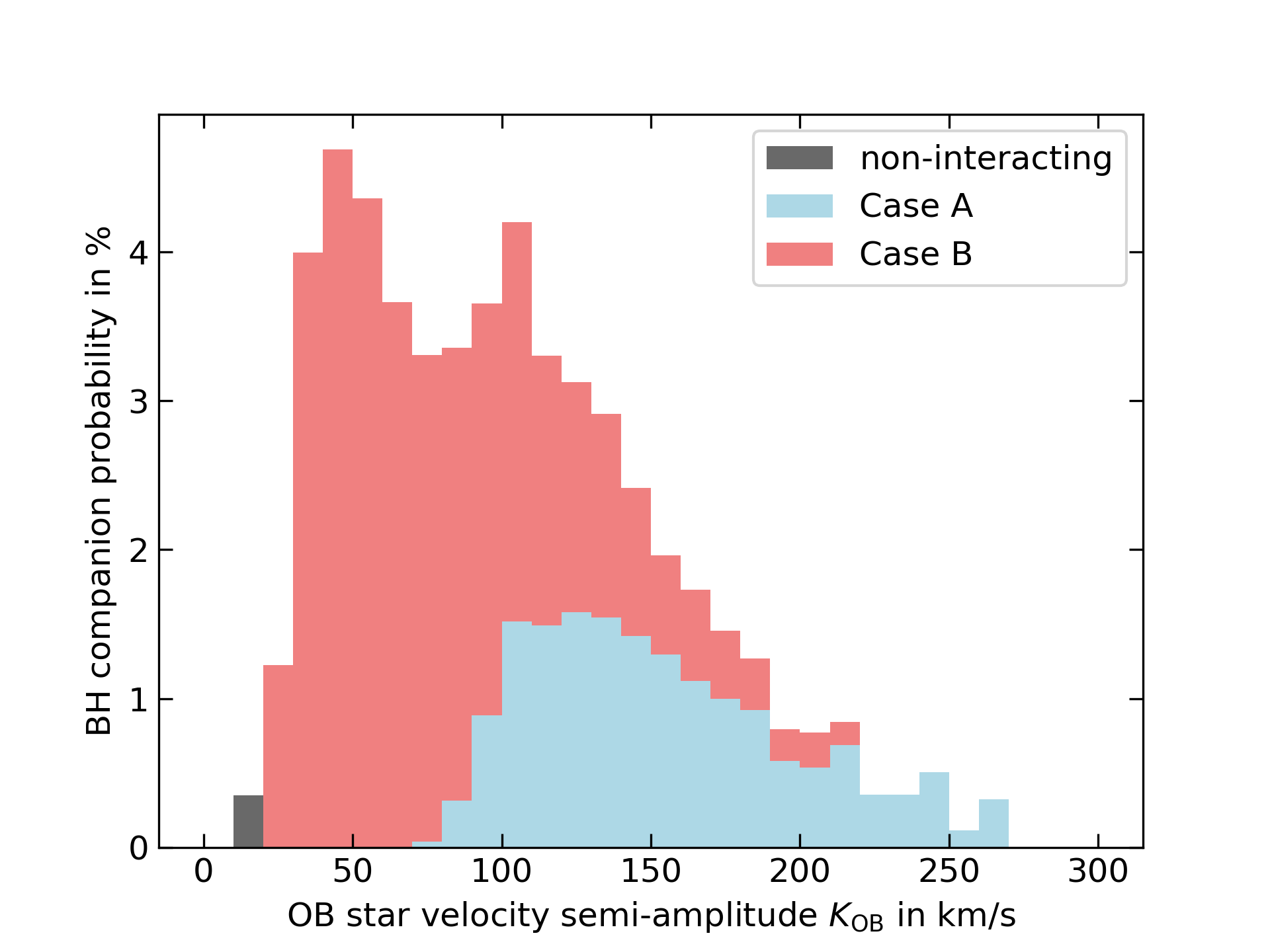
Figure 12: Prediction of our population synthesis model for the probability of OB stars to have a BH companion, as function of the observed orbital period (top), and the observed radial velocity semi-amplitude (bottom), respectively.

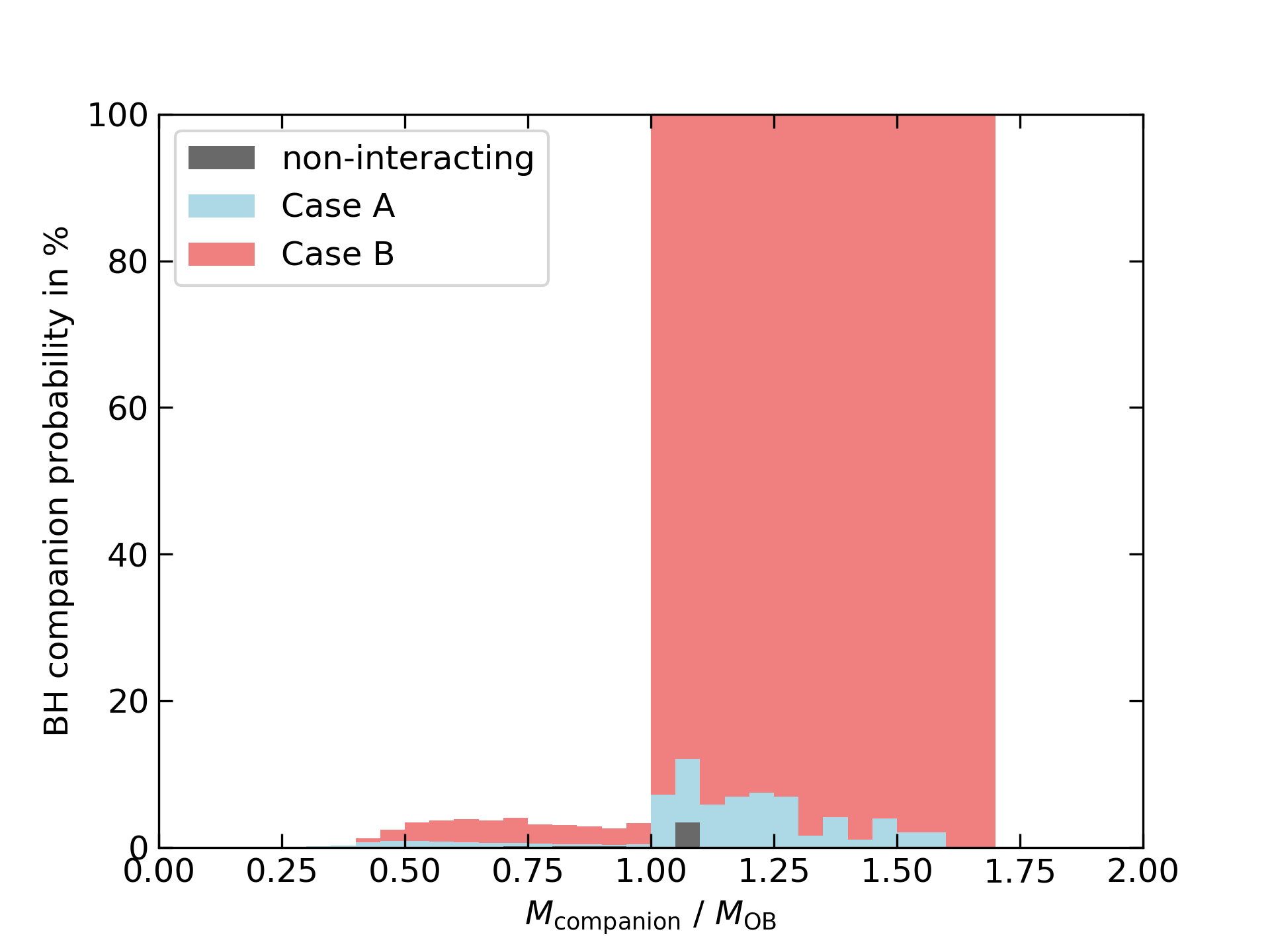
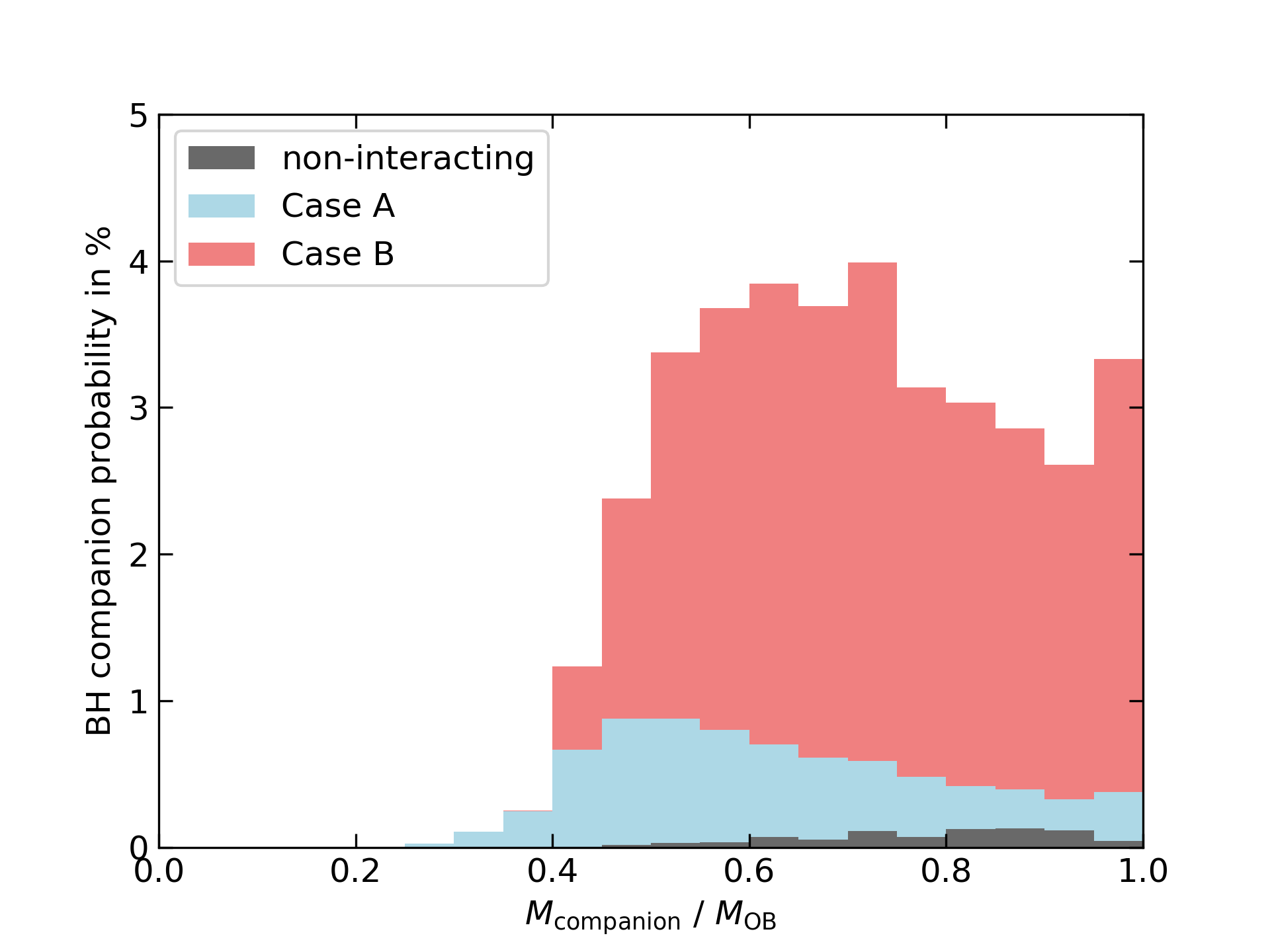
Figure 13: Prediction of our population synthesis model for the probability of a randomly picked OB binary to have a BH companion, as function of the mass ratio (top). Here, a mass ratio above one means the BH is heavier than the OB star; if such an OB binary is picked, its probability of having a BH companion is one. The bottom panel shows a zoom of the part with a mass ratio less than one.

Figure 13 gives the probability of a randomly picked OB binary to be accompanied by a BH as function of the mass ratio $q=M_{\rm companion}/M_{\rm OB}$. Note that for $q>1$, this probability is one. In this case the companion must be a BH and can not be an ordinary star, since otherwise the ordinary companion star would be the more luminous star of the two, and it would have been picked as the primary OB star.

We see that the smallest mass ratios are dominated by Case A systems, which is a consequence of the rather high accretion efficiency in those; i.e., the OB stars in such binaries did gain substantial amounts of mass. Combined with Fig. 12, this means that the OB+BH binaries with the lowest mass ratios have small orbital periods.

Finally, Fig. 13 shows that the largest mass ratios produced by our model binaries is about $q=1.7$. Binaries with such high mass ratios originate from OB+OB binaries with initially massive primaries and extreme mass ratio, e.g., $40\,\mathrm{M}_{\odot}+13\,\mathrm{M}_{\odot}$, in which the secondary accretes little material. The OB stars in such systems are therefore expected to be be early B or late O stars.

Above, we have discussed the BH companion probabilities of randomly picked OB stars, and found them to be of the order of a few percent. Considering observing campaigns to search for OB+BH binaries, an efficiency of a few percent is rather low. However, the OB stars in OB+BH binaries have had a turbulent life, and signs of that may still be visible. In particular, all OB stars in our OB+BH model binaries have accreted some amount of matter from their companion. As the accretion efficiency in our models drops once the mass gainer has reached critical rotation, and since a mass increase by about 10% is required to achieve this (Packet 1981, Petrovic et al. 2005), this is roughly the minimum mass increase of our OB mass gainers.

From the properties of the OB stars in OB+BH binaries as described in Sect. 3, we see most OB stars with a BH companion are expected to stand out amongst the ordinary OB stars. In Case A systems, the OB star rotation is expected to be relatively fast, but since only the projected rotation velocity can be easily measured, this is not an unambiguous selection criterion. However, in our models, the BH companion induces a radial velocity variation of 200$\,{\rm km}\,{\rm s}^{-1}$ or more ($K\mathrel{\hbox{\hbox to0.0pt{\hbox{\lower 4.0pt\hbox{$\sim$}}\hss}\hbox{$>$}}}100\,{\rm km}\,{\rm s}^{-1}$; Fig. 8), which should be easily seen even though the observed value will again be smaller due to projection (by 21% on average). In addition, our models predict a significant surface enrichment with products of hydrogen burning in the fast majority of all cases, the strongest signature being a clear nitrogen enrichment.

In the Case B binaries, surface enrichment of the OB components is predicted to be small. However, their rotation velocity is expected to exceed 300$\,{\rm km}\,{\rm s}^{-1}$, with values close to critical rotation in those with masses below $\sim 20\,\mathrm{M}_{\odot}$. And even in Case B, the expected radial velocity variations of the OB stars exceed $40\,{\rm km}\,{\rm s}^{-1}$, with an average well above $100\,{\rm km}\,{\rm s}^{-1}$.

We note that also the mass ratios of our OB+BH binaries are rather favourable. That means, if we assume that a MS companion would still be detected as such for mass ratios above 0.5, then such a companion could be excluded in potential observations of almost all of our OB+BH model binaries. Given the clues accumulated above, a corresponding search for BHs in SB1 spectroscopic binaries might thus be promising.

Finally, we want to emphasise that additional possibilities to identify potential OB+BH binaries exist when considering the population of young star clusters. In particular, many of the OB stars in our OB+BH model binaries which evolved via Case A mass transfer have gained a substantial amount of mass. The mass increase may lead the stars appear above the cluster turn-off, and the convective core mass increase will rejuvenate them such that they appear younger than most other cluster stars (van Bever & Vanbeveren 1997, Schneider et al. 2014, Wang et al. 2020).

8 Further evolution and connection to double compact mergers

As shown in Fig. 1, the OB+BH stage on which we focus here is the last evolutionary stage of massive binaries which, so far, can be reached with detailed calculations from the ZAMS. Therefore, predictions for later stages become more and more uncertain, and are not derived from our models. Nevertheless, it is interesting to speculate about the future evolution of the OB+BH.

First of all, due to the rather large orbital periods of our OB+BH systems (Fig. 6), in almost all of our model binaries the OB star would fill its Roche-volume only after core hydrogen exhaustion (Case B). We would therefore expect a thermal timescale mass transfer from the OB star to the BH, with a mass transfer rate of $\dot{M}\simeq LR/(GM)$. Since this stage is very short ($\sim 10^{4}\,$yr), we would expect to observe only very few systems in this stage, SS 433 perhaps being one of them (Hillwig & Gies 2008). It depends on the mass ejection rate from the mass transferring binary whether a common envelope evolution is initiated or avoided at this stage. For smaller periods and rather low mass donors, it can perhaps be avoided as estimated by King et al. (2000) for SS 433, which has an orbital period of $13.1\,$d and for which a mass ejection rate of the order of $10^{-4}\,\,\,\mathrm{M}_{\odot}\leavevmode\nobreak\ {\rm yr}^{-1}$ has been determined. For the bulk of our systems, the stellar radius and luminosity will be much larger, and the mass transfer rate would typically be $10^{-2}\,\,\,\mathrm{M}_{\odot}\leavevmode\nobreak\ {\rm yr}^{-1}$, such that common envelope evolution appears more likely. With the assumptions for the common envelope evolution as in Kruckow et al. (2016), except for possibly the widest systems, we would expect a merging of both stars.

In any case, the accretion of matter of BHs inside a stellar envelope, and the common envelope evolution of a BH and a non-degenerate star, can not yet be predicted with certainty. Therefore, whether there is a critical orbital period in our predicted OB+BH period distribution (Fig. 6) beyond which the systems survive the common envelope evolution as a binary, and what its value would be, remains open. The fact that the peak of the period distribution corresponds to a rather large value ($\sim 200\,$d) leaves room for the speculation that a significant fraction of the OB+BH binaries will lead to tight double BH systems.

9 Conclusions

In this paper, we have provided predictions for the properties of the OB+BH binary population in the LMC. These predictions are based on almost 50 000 detailed binary evolution models. These models include internal differential rotation, mass and angular momentum transfer due to Roche-lobe overflow, and no inhibition of envelope inflation due to the Eddington limit. Only models which undergo stable mass transfer are considered, implying that common envelope evolution may add additional OB+BH binaries to our synthetic population. Our results are subject to substantial uncertainties, which we discuss in detail in Sect. 4. However, they represent the last long-lived stage of massive binaries on their way to double compact binaries that can be modeled in detail without interruption starting from the double main sequence stage, which allows the prediction of their properties with a rather limited amount of assumptions (Sect. 2). This includes the initially closest binaries which undergo mass transfer during hydrogen burning (Case A), which can be treated only rudimentary in rapid binary evolution calculations.

We compare our predictions with the number and properties of the observed OB+WR binaries in the LMC, which may be the direct progenitors of OB+BH binaries. We find good agreement with the mass distribution and with the orbital period distribution up to $\sim 40\,$d. However, there is a lack of observed long period ($\sim 100\,$d) OB+WR binaries and of B+WR binaries, compared to our predictions. While the corresponding observational biases are not well understood, the similarity of the observed Be/X-ray binary period distribution to that predicted for the OB+BH binaries argues for the so far undetected presence of long-period unevolved binary companions in a significant fraction of the WR star population.

We derive the distribution of masses, mass ratios, and orbital periods of the expected OB+BH binary population, and show that OB stars with BH companions may be identified through their radial velocity variations, their rotation rate or their surface abundances. Our results imply that an average O or early B star in the LMC has a BH companion with a probability of a few percent, which argues for about 120 OB+BH binaries currently in the LMC. With an about five to ten times higher star-formation rate, the Milky Way may thus harbour around 1000 of such system. All together, only four such binaries have been found so far, with one of them in M33.

The vast majority of the predicted OB+BH binaries are expected to be X-ray quiet. The reason is that due to their rather large expected orbital periods (Fig. 12), wind material may be accreted in an advection-dominated flow rather than via an accretion disk. This picture is confirmed by the Be-BH binary MCW 656 which has an orbital period of 60 d. In any case, we have shown that the expected orbital velocities are sufficiently large to identify OB+BH binaries spectroscopically (Fig. 12) — which is easier here than in their OB+WR progenitors —, that the mass ratios are such that main sequence companions can easily be excluded, and that rapid rotation and/or chemical surface enrichment may help to identify candidate systems.

We find the accumulated evidence for a so far undetected large population of OB+BH binaries significant. Its discovery would largely help to reduce the uncertainty in massive binary evolutionary models, and pave the way to understand the contribution of close binary evolution to the BH-merger events observed through their gravitational wave emission.

Appendix A Self-lensing of OB+BH binaries

The presence of a black hole can potentially be verified by gravitational lensing magnification. Provided the OB star is sufficiently well aligned behind the observer–black hole sightline, the black hole can cause a magnification on the star’s flux (Masuda & Hotokezaka 2019, D’Orazio & Stefano 2020). This lensing magnification would show up as a symmetric peak in the light curve of the OB star once per orbit. The maximum magnification is obtained if star, black hole, and observer are perfectly aligned, and for star of radius $R_{*}$ with uniform surface brightness, its value is $\mu_{\rm max}=\rho^{-1}\sqrt{4+\rho^{2}}$, where $\rho=R_{\rm OB}/R_{\rm E}$ is the ratio of stellar radius and Einstein radius. Since the distance of the binary system is much larger than the orbital radius $a$ of the binary, the Einstein radius for a black hole of mass $M_{\rm BH}$ is

$$R_{\rm E}\approx\sqrt{{4GM_{\rm BH}\over c^{2}}\,a}\approx 7.7\times 10^{9}\,{\rm cm}\left({M_{\rm BH}\over 10\,{\rm M}_{\odot}}\right)^{1/2}\left({a\over 10^{13}\,{\rm cm}}\right)^{1/2}\;.$$

Therefore, the dimensionless stellar radius $\rho$ becomes

$$\rho\approx 65\left({R_{\rm OB}\over 5\times 10^{11}\,{\rm cm}}\right)\left({M_{\rm BH}\over 10\,{\rm M}_{\odot}}\right)^{-1/2}\left({a\over 10^{13}\,{\rm cm}}\right)^{-1/2}\;,$$

and is thus $\gg 1$. Hence, we can expand the maximum magnification to yield a maximum brightening of the star by

$$|\Delta m|_{\rm max} = 1.086\,\ln\mu_{\rm max}\approx{2.17\over\rho^{2}}$$ (1)

$$\approx 5.2\times 10^{-4}\left({R_{\rm OB}\over 5\times 10^{11}\,{\rm cm}}\right)^{-2}\left({M_{\rm BH}\over 10\,{\rm M}_{\odot}}\right)\left({a\over 10^{13}\,{\rm cm}}\right)\;.$$

Thus, the maximum brightness increase of the star is of the order of a milli-magnitude for the fiducial parameters, and scales linearly with the orbital radius and black hole mass. The magnification decreases with the misalignment of star, black hole and observer, such that it drops to about half the value given in Eq. (1) when the star is misaligned by approximately its own radius. Requiring that the star passes behind the black hole with a misalignment not larger than its own radius puts a constraint on the inclination angle $i$ of the orbital plane of the binary, $\sin(i)\lesssim R_{*}/a$, or

$$i\lesssim 2.85\,{\rm deg}\left({R_{\rm OB}\over 5\times 10^{11}\,{\rm cm}}\right)\left({a\over 10^{13}\,{\rm cm}}\right)^{-1}\;.$$

Thus, the orbital plane needs to be well aligned with the sightline to the binary system in order to yield a brightening larger than $\sim 0.5|\Delta m|_{\rm max}$.

The prospects for observing lensing magnification in such binary systems depends sensitively on the photometric accuracy with which the light curve can be recorded. The lensing nature of the magnification peaks can be further verified by spectroscopic studies: since the OB star is predicted to rotate rapidly, the shape of spectral lines will change during the magnification event, since stellar surface regions with approaching and receeding (rotational) velocity will be magnified consecutively. Hence, we expect to see a characteristic time variability of spectral shapes during the magnification event.

Verifying a lensing event places a strong constraint on the object causing the lensing – it has to be smaller than the Einstein radius.

Appendix B Outcome of the binary models for four additional primary masses