Initial Evaluation of SNEMO2 and SNEMO7 Standardization Derived From Current Light Curves of Type Ia Supernovae

Abstract

To determine if the SuperNova Empirical Model (SNEMO) can improve Type Ia supernova (SN Ia) standardization of several currently available photometric data sets, we perform an initial test, comparing results with the much-used SALT2 approach. We fit the SNEMO light-curve parameters and pass them to the Bayesian hierarchical model UNITY1.2 to estimate the Tripp-like standardization coefficients, including a host mass term as a proxy for astrophysical systematics. We find that, among the existing large data sets, only the Carnegie Supernova Project data set consistently provides the signal-to-noise and time sampling necessary to constrain the additional five parameters that SNEMO7 incorporates beyond SALT2. This is an important consideration for future SN Ia surveys like LSST and WFIRST. Although the SNEMO7 parameters are poorly constrained by most of the other available data sets of light curves, we find that the SNEMO2 parameters are just as well-constrained as the SALT2 parameters. In addition, SNEMO2 have comparable intrinsic scatter when fitting the same data. It is not then, the SNEMO methodology, but the interplay of data quality and the increased number of degrees of freedom that is behind these reduced constraints. With this in mind, we recommend further investigation into the possibility of fitting the poorer photometry data with intermediate SNEMO-like models with three to six components.

1 Introduction

Observations show that measurable properties of Type Ia supernovae (SNe Ia) are correlated with their peak brightnesses, making SNe Ia standardizable candles (Phillips, 1993; Hamuy et al., 1996; Riess et al., 1996; Perlmutter et al., 1997). Once their peak brightnesses are standardized, they can be used as distance indicators and aid in our understanding of the expansion history of universe. The precision with which cosmological parameters are constrained depends, in part, on how well SN Ia standardization reduces the dispersion in peak brightnesses. Beginning in the 1990s, standardization techniques were developed that reduced the dispersion to 0.15 mag, resulting in the discovery of the accelerating expansion of the universe (Riess et al., 1998; Perlmutter et al., 1999). Since then, improving techniques for SN Ia standardization has been a continuous topic of research. (e.g. Phillips et al., 1999; Guy et al., 2005; Jha et al., 2007; Guy et al., 2007; Burns et al., 2011). Further improvements may be needed in order to remove possible percent level systematics (e.g. Foley & Kasen, 2011; Kim et al., 2013; Fakhouri et al., 2015; Pierel et al., 2018; Burns et al., 2018; Hayden et al., 2019) that could affect measurement of Dark Energy by future missions like LSST (LSST Science Collaboration, 2009) and WFIRST (Spergel et al., 2015; Hounsell et al., 2018).

SNe Ia are typically observed photometrically in a few broadband optical filters with an observation every few days. The resulting light curves are then fit to one of several empirically-based models in order to extract SN Ia parameters that quantify properties like light-curve shape and color. These parameters are then used to standardize the absolute luminosity of the supernovae , measure distances, and eventually constrain cosmological parameters. The exact interpretation of these parameters differs for each light-curve fitting method.

Light-curve fitters like Hamuy et al. (1996), Riess et al. (1996), Phillips et al. (1999), and Jha et al. (2007) use a single light-curve shape parameter and separate the sources of SN Ia color variation by assuming a fixed Milky Way extinction curve to describe the dust and attributing the remaining color variation to intrinsic color differences in the SNe Ia. Tripp (1998) and Guy et al. (2007) also use a single light-curve shape parameter, but do not separate the sources of color variation. The popular SALT2 (Guy et al., 2007, 2010; Betoule et al., 2014; Mosher et al., 2014) uses a linear model of the SN Ia spectral energy distribution sequence fit from light curves and spectra. The model is parameterized by finding the coefficients that produce synthetic photometry most similar to the observed photometry. One parameter, $x_{1}$, captures the broader-brighter (or Phillips) relationship identified in Phillips (1993) and Pskovskii (1977). For normal SNe Ia, $x_{1}$ roughly follows a standard normal distribution. The second parameter, $c$, accounts for color variability both from dust and intrinsic diversity. For typical SNe Ia, $c$ is within a few tenths of a magnitude of zero.

The standardization method commonly referred to as Tripp standardization (Tripp, 1998), combines these light-curve shape and color parameters linearly to estimate the distance modulus, $\mu$. This is typically done for the rest-frame $B$-band magnitude ($m_{B}$). Using the parameters from the SALT2 SN Ia light-curve model, the Tripp standardization equation is:

$$\mu=m_{B}-(M_{B}-\alpha\;x_{1}+\beta\;c)$$ (1)

where $\mu$, $m_{B}$, $M_{B}$ are the distance modulus, apparent magnitude, and absolute magnitude respectively. The $\alpha$ and $\beta$ parameters are the linear standardization coefficients corresponding to the SN Ia light-curve shape ($x_{1}$) and intrinsic color ($c$). The parameters $m_{B}$, $x_{1}$, and $c$ are fit for each individual SN Ia, while $M_{B}$, $\alpha$, and $\beta$ are global parameters that are fit simultaneously, along with the cosmological parameters of interest, using the full data set.

There is evidence suggesting that SNe Ia show considerably more spectral diversity than the shape and color parameters capture (Branch et al., 2006; Kim et al., 2013; Fakhouri et al., 2015; Hayden et al., 2019; Rubin, 2019). This diversity may present itself as uncorrected systematic shifts in the peak luminosity of SN Ia. An example of such an unaccounted for systematic is seen in the host galaxy mass step (Kelly et al., 2010; Sullivan et al., 2010; Lampeitl et al., 2010). The mass step is a shift in average peak luminosity of $\sim 0.06~{}\text{mag}$ between SN Ia from low stellar mass host galaxies ($\lesssim 10^{10}~{}\text{M}_{*}/\text{M}_{\odot}$) to high mass hosts ($\gtrsim 10^{10}~{}\text{M}_{*}/\text{M}_{\odot}$). This result has been seen in multiple samples with a $>5\sigma$ significance (Childress et al., 2013; Uddin et al., 2017; Moreno-Raya et al., 2018).

1.1 SNEMO

In order to address the issue of unmodeled spectral diversity, Saunders et al. (2018) presented the Super-Nova Empirical MOdels (SNEMO), which applies expectation maximization factor analysis (EMFA, a dimensionality reduction algorithm similar to principal component analysis) to optical spectrophotometric time series obtained by the Nearby Supernova Factory (SNfactory, Aldering et al. 2002). EMFA reduces the dimensionality of the training data set to a predefined number of eigenvectors. In the case of SNEMO, these eigenvectors are time series of spectra (Saunders et al., 2018, Equations 7 & 10). Combined, these eigenvectors represent a linear basis from which one can reconstruct any optical SN Ia spectral time series. This method of defining the eigenvectors is similar to the method used to define SALT2’s $x_{1}$ (Guy et al., 2007, Section 5), however SNEMO handles missing and noisy data in a different manner and does not use any photometric data. SNEMO does not fit a variable color law and instead assumes a Fitzpatrick & Massa (2007) reddening law (Saunders et al., 2018, Section 3.2). Like SALT2, each of the best-fit model coefficients (or eigenvector projections) describe a certain light-curve shape and can be combined to standardize supernova magnitudes. Unlike some light-curve shape parameters (e.g. $\Delta m_{15}$), these EMFA eigenvectors are pure mathematical constructs and do not necessarily connect to anything physical or intuitive.

SNEMO is a family of models trained on the same data. Saunders et al. (2018) released three variants: SNEMO2, SNEMO7, and SNEMO15 . SNEMO2 is named for its two spectral-temporal eigenvectors; SNEMO7 and SNEMO15 have seven and fifteen eigenvectors respectively. In addition, each SNEMO model has a color correction curve that is identical to the Fitzpatrick & Massa (2007) reddening law. The “zeroth” eigenvector, describing the mean spectral-temporal evolution, is related to $m_{B}$ in Equation 1, and its corresponding coefficient used only as an overall scaling factor. The other spectral-temporal and color parameters are combined linearly to standardize SNe Ia.

SNEMO2, which consists of a mean vector, one spectral-temporal component of variation, and a color law, is directly analogous to SALT2, differing only in the training data and methodology . SNEMO2 allows a direct comparison between the SNEMO and SALT2 training methodologies without introducing any more degrees of freedom . The other SNEMO models introduce more parameters to allow the model to capture more of the spectral variation. In the initial release of SNEMO, Saunders et al. (2018) showed that these extra parameters do improve the quality of the model in fitting the diversity of SN Ia behavior.

Using the SNfactory training and a separate SNfactory validation set, SNEMO15 was found to be the model able to capture the most spectral diversity while avoiding overfitting. SNEMO7 was considered to be a model that well-sampled multi-band light curves should be able to constrain, while capturing more SN Ia variation than SNEMO2 (or SALT2). In addition, SNEMO7 was determined to be the point of diminishing returns when using Tripp-like linear standardization. It is worth noting that there is evidence for non-linear behavior that may require the more descriptive spectral fits obtained with SNEMO15.

Figure 1:

In this work, we perform the initial test of how well SNEMO7 standardizes SNe Ia using only publicly available photometric light-curve data. This goes beyond the spectrophotometric time series data set used in the development and initial testing . We include a host stellar mass term as a proxy for any uncorrected SN Ia astrophysical systematics. It is these possible unknown systematics that stand as the largest threat to precision Dark Energy measurements. Host stellar mass has become a standard proxy . However more recent research by Gupta et al. (2011), Hayden et al. (2013), Rigault et al. (2013), Childress et al. (2013), Childress et al. (2014), Moreno-Raya et al. (2018), Rigault et al. (2018), Rose et al. (2019), and others show that alternative astrophysical measurements may better match the true physical mechanism.

We use the following criteria to evaluate SNEMO7’s ability to standardize current data sets:

1. When applying the model to current light-curve-only data, are the standardization coefficients consistent with those derived from the training data set?

2. How many standardization coefficients are distinguishable from zero?

3. What are the correlations between the coefficients? Strong correlations imply that a projection needs to be fit even if the standardization coefficient is consistent with zero.

4. Given current data sets, does SNEMO7 reduce the need for unexplained intrinsic scatter in SN Ia ($\sigma_{\rm unexplained}$) in the Hubble-Lemaître diagram?

5. Does SNEMO7 reduce the correlations with host-galaxy properties, such as the one with stellar mass ($\gamma$)? A reduction of these correlations would imply a reduced systematic floor for SN Ia standardization.

These tests do not attempt to validate or characterize SNEMO’s ability to fit light curves, but rather focus on questions concerning cosmological measurements. Characterizing light curve fits will be done thoroughly in a forthcoming paper (Saunders et al. 2020). We will also not investigate the limits of Tripp-like standardization equations or methods. Finally, we are here only asking how SNEMO fares on these 5 criteria when given the current quality of SN Ia data sets, not how it performs when given the data quality expected from LSST or WFIRST. These are all important research topics and should be discussed independently.

In Section 2, we discuss the photometric data and the method we used to test SNEMO7, and in Section 3, we discuss our findings and present answers the five questions above.

2 The Data and UNITY

This work uses high-redshift ($z\gtrsim 0.5$) Hubble Space Telescope (HST) data from Riess et al. (2007), mid-redshift ($0.1\lesssim z\lesssim 0.4$) data from the rolling supernovae surveys of the Sloan Digital Sky Survey (SDSS, Sako et al. 2014) and the ($0.1\lesssim z\lesssim 1.0$) Supernova Legacy Survey (SNLS, Betoule et al. 2014), and nearby ($z<0.1$) SNe Ia observed with targeted followup from the Foundation survey (Foley et al., 2018), the Carnegie Supernova Project (CSP) third data release (Krisciunas et al., 2017), and the Center for Astrophysics Fred Lawrence Whipple Observatory Supernovae data releases (CfA, Riess et al., 1999; Jha et al., 2006; Hicken et al., 2009, 2012). Of these many data sets, CSP followed the SNe Ia at a faster cadence than most and obtained observations with higher-than-typical signal-to-noise. We use only objects with available host galaxy stellar mass measurements (Gupta et al. 2020). The number of SNe Ia from each survey are in Table 1. The total size of the sample with host galaxy stellar mass measurements is 914.

Table 1: Number of SN Ia passing quality cuts from various SNEMO models.

	CSP	Foundation	CfA	SDSS	SNLS	HST	Total
Total SNe	134	223	97	371	239	9	1073
Host mass avail.	99	99	97	371	239	9	914
		SNEMO2
No Error Model
$\sigma_{i}\leq 2$	96	99	95	355	234	6	885
1% Error Model
$\sigma_{i}\leq 2$	96	98	96	355	234	7	886
2% Error Model
$\sigma_{i}\leq 2$	97	98	94	352	234	6	881
		SNEMO7
No Error Model
$\sigma_{i}\leq 1$	80	36	16	12	13	0	157
$\sigma_{i}\leq 2$	83	62	45	24	26	0	240
1% Error Model
$\sigma_{i}\leq 1$	66	9	4	11	0	0	90
$\sigma_{i}\leq 2$	75	52	28	21	18	0	194
2% Error Model
$\sigma_{i}\leq 1$	36	0	1	2	0	0	39
$\sigma_{i}\leq 2$	73	22	9	15	7	0	126

Note. — $\sigma_{i}$ is the uncertainty on each fit eigenvector. When $\sigma_{i}=1$, the uncertainty is approximately the $1\sigma$ dispersion in the population. The data from the CfA, SDSS, SNLS, and HST surveys were obtained via the JLA compilation (Betoule et al., 2014).

2.1 SNEMO7 Light-Curve Fits

The SNEMO models are available in the sncosmo python package (version 1.7). We use the mcmc_lc function in that package to find the posterior distribution of the best-fit model coefficients (i.e. the eigenvector projections, $c_{i}$) and estimate their uncertainties ($\sigma_{i}$) from these posteriors. This function uses MCMC to sample from

$$\chi^{2}={(\mathbf{f}_{\mathrm{obs}}-\mathbf{f}_{\mathrm{mod}})^{\top}}(\Sigma_{\mathrm{obs}}+\Sigma_{\mathrm{mod}})^{-1}(\mathbf{f}_{\mathrm{obs}}-\mathbf{f}_{\mathrm{mod}})\;.$$ (2)

This is a function of the model coefficients $(z,t_{0},c_{i},A_{s})$, where $\mathbf{f}_{\mathrm{obs}}(b,p)$ is the flux observed in bandpass $b$ at phase $p$ and $\mathbf{f}_{\mathrm{mod}}(b,p;z,t_{0},c_{i},A_{s})$ is the flux predicted in bandpass $b$ at phase $p$ obtained by performing synthetic photometry on the spectral time series model with the given model coefficients. A diagonal covariance matrix whose entries represent the observational uncertainty ($\Sigma_{\mathrm{obs}}$) is added to the model covariance ($\Sigma_{\mathrm{mod}}$) . The population dispersion of a given component ($c_{i}$) is normalized to approximately 1, meaning $\sim$ 1,000 normal SNe Ia should have a $c_{i}$ range of $\sim$ $-3$ to $3$. Further details on the interpretation of SNEMO parameters can be found in Saunders et al. (2018). In addition to the SNEMO coefficients, the time of maximum brightness is fit along with the model coefficients with wide, uniform priors ($(-50,50)$ for each of the model coefficients, and $(\min(t_{\mathrm{obs}})-20,\max(t_{\mathrm{obs}}))$ for the time-of-max). When running the inference, we let the redshift in SNEMO vary within the uncertainty of the measurement ($\sim$ 0.0001). We also correct for Milky Way dust reddening using the Schlafly & Finkbeiner (2011) maps.

In a SALT2-like analysis, initial light-curve quality cuts based on phase sampling and signal-to-noise are usually applied. We do not yet have a similar heuristic for which light curves are high enough quality to fit with SNEMO7. Instead, we filter the SNe Ia on the SNEMO7 parameters and uncertainties directly, rather than any other measured properties of the light curves. We define an object to be well fit by SNEMO7 when its eigenvector coefficient values are less than a threshold ($|c_{i}|<5$) and the uncertainties on those coefficients are also smaller than another threshold ($\sigma_{i}\leq 2$). The cut on $|c_{i}|<5$ is intended to remove large outliers, and the cut on $\sigma_{i}>2$ removes SN Ia that have an uncertainty in the best-fit coefficients larger than twice the $1\sigma$ population dispersion. A high $\sigma_{i}$, e.g. $>2$, represents data that can be fit by a wide range of models, effectively putting no constraint on the true values of the model parameters. We investigate the effect of different $\sigma_{i}$ cutoff values on our results in Appendix A. These quality cuts remove unconstrained fits without excessively restricting our sample size. This results in a data set of $N=240$.

SNEMO7 does not yet have an uncertainty model (the $\Sigma_{\mathrm{mod}}$ in Equation 2). A formal uncertainty model describes the regions in parameter space where SNe Ia are more diverse than the model and reduces the impact these regions have on fitting data. This uncertainty model is under development (Saunders et al. 2020), but we need to look at the effect of treating the model as imperfect. For SALT2, the uncertainty model is partially determined by the statistical uncertainty from their training data set (Guy et al., 2007); the model is more certain in areas that had more training data. For SNEMO, the training data was selected to all have the same rest-frame wavelength coverage. As such, this part of the uncertainty model should be smooth. The other part of the SALT2 uncertainty model describes correlated residuals around the model. We expect this component to be reduced for SNEMO7, as it describes more of the intrinsic SN behavior. Using these assumptions, we investigate the effects of an imperfect model using a simplified uncertainty model. This naive uncertainty model consists of a diagonal covariance matrix with entries given by 1% or 2% of the peak flux value in each band. The formal uncertainty model in development, has more variation in phase than our naive model, but its scale is with in this range.

The addition of these uncertainties degrades the coefficient measurement precision , therefore reducing the number of SN Ia passing quality cuts. With a 1% naive uncertainty model, the number of SN Ia passing our quality cuts are $N=194$, and dropping to $N=126$ with the 2% uncertainty model. Ultimately, the data sets that survive these cuts are dominated by CSP SNe Ia.

Several factors contribute to the poor constraints on the model parameters. A large factor is wavelength coverage. The SNEMO model is defined from 3300–8600 Å, and any observations in bands with rest-frame wavelengths outside of this range are not used to constrain the model parameters. As an example, we find that all of the SNLS objects that pass our cuts are at redshifts below $\sim 0.7$, which is where the effective wavelength of the $r$-band falls below the lower bound of the SNEMO wavelength range. The signal-to-noise ratio of the observations or the temporal sampling of the light curves can also have an impact on our ability to constrain the model parameters in the light curve fits. A full study of these effects is left to future work.

2.2 UNITY1.2

We used the Unified Nonlinear Inference for Type Ia cosmologY (UNITY) framework to estimate the standardization equation. UNITY, a Bayesian hierarchical model implemented in Stan (Carpenter et al., 2017) using pystan (10.5281/zenodo.598257), was developed by Rubin et al. (2015) and further refined by Hayden et al. (2019). A more recent version (UNITY1.2) now includes the capability of modeling Tripp-like standardization equations with an arbitrary number of standardization parameters. Because our focus is on standardization and not cosmology directly, we assume a flat, $\Lambda$CDM cosmology with $\Omega_{M}=0.3$.

Using the SNEMO7 model with UNITY requires a total of eight standardization coefficients: six for the light-curve-shape eigenvectors, one for the color law, and finally a coefficient describing the effect (if any) of host galaxy stellar mass. These can be combined into a standardized distance modulus equation, following the Tripp convention:

$$\mu=m_{B}-\Big{(}M_{B}+\beta A_{s}+\gamma m+\sum_{i=1}^{N}\alpha_{i}c_{i}\Big{)}$$ (3)

where $\mu$, $m_{B}$, $M_{B}$ are the distance modulus, apparent and absolute magnitude respectively, the same as Equation 1. For SALT2 and SNEMO2, $N=1$, but for SNEMO7, $N=6$. $A_{s}$ and $\beta$ are the color term and color standardization coefficient respectively. $A_{s}$ is a spectral variant of the traditional $A_{\rm V}$ extinction. For comparison to SALT2, $A_{s}$ should be approximately $(R_{V}+1)c$, meaning that $\beta$ should be $\sim 1$. Finally, $\gamma$ is the standardization coefficient applied to the logarithm of the stellar host galaxy stellar mass ($m$). The zero point of $m$ is shifted such that the data set’s average is zero, partially decorrelating $\gamma$ and the absolute magnitude $M_{B}$. As this standardization equation uses the same sign for all of the coefficients, these $\alpha$ coefficients have the opposite signs as the one in Equation 1. Due to the small sample sizes, we ran UNITY1.2 without estimating selection effects or calibration offsets between data sets.

2.3 SALT2 Fit as a Reference

In order to test if SNEMO can improve the Hubble-Lemaître diagram unexplained dispersion or reduce the correlations with host-galaxy properties, we first need a baseline for our comparison. As such, we use the SALT2.4 version of SALT2 to fit the SNe Ia that passed basic quality cuts for SNEMO2 and SNEMO7. The results were then put into UNITY1.2 to estimate the standardization coefficients of Equation 3. The nominal value for a SALT2 Tripp-like mass standardization parameter, with the data set that can constrain SNEMO7, was found to be $\gamma=-0.01\pm 0.02$. The full fit can be seen in Figure 2 with the numerical values presented in Tables 2 and 3.

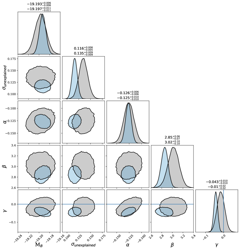
Figure 2: A corner plot of the posterior distribution for the SALT2 standardization parameters: the peak luminosity of SN Ia (${\rm M}_{B}$), the unexplained scatter in magnitudes ($\sigma_{\rm unexplained}$), and the standardization coefficients ($\alpha$, $\beta$, and $\gamma$ from Equation 3). Grey contours are for the data set that passed the $\sigma_{i}\leq 2$ quality cuts with SNEMO7 ($N=240$) whereas the blue contours are for the SN Ia that passed the same cuts when fit with SNEMO2 ($N=867$). Each marginalized distribution’s median, along with $1\sigma$ uncertainties, are numerically represented above the corresponding histogram; top and bottom numbers are for the blue and grey distributions, respectively. The location of a null host galaxy standardization is shown via the blue line. All two-dimensional contours show 2$\sigma$ confidence regions. This posterior distribution is consistent with previously published estimates (Sullivan et al., 2010; Betoule et al., 2014; Scolnic et al., 2018).

3 Results & Discussion

3.1 SNEMO2

Our first objective was to test the modeling methodology used by SNEMO . With only two model parameters to fit, SNEMO2 allows for a direct comparison between SALT2 and SNEMO. Figure 3 shows the resulting posterior, as inferred by UNITY1.2, for the SNEMO2 standardization equation. Numerical values are presented in Table 2.

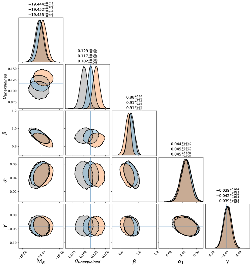
Figure 3: Same as Figure 2, but using the SNEMO2 light curve fitter. Three different uncertainty models are shown: no uncertainty model (orange), 1% of peak uncertainty floor (blue), and a 2% uncertainty (gray). Each parameter is well constrained independent of the assumed uncertainty model. As expected, the intrinsic scatter ($\sigma_{\rm unexplained}$) depends directly on the uncertainty model. When the uncertainty model decreases to zero (orange contours) the unexplained scatter increases to compensate. The stellar mass dependence is very consistent with what is seen when using SALT2. The blue lines for the $\sigma_{\rm unexplained}$ and $\gamma$ are the medians of the SALT2 analysis of the same data set. Like Figure 2, the median and $1\sigma$ uncertainties for the marginalized distributions are numerically presented above the associated histograms, first for the no uncertainty model (orange), then for the 1% of peak uncertainty floor (blue), and finally for the 2% uncertainty floor (gray).

SNEMO2’s standardization parameters are well constrained and independent of the uncertainty model. Each data set analyzed corresponds to one of the three different uncertainty models, uses our default quality cuts of $\sigma_{i}\leq 2$ and $|c_{i}|<5$, and includes more than 800 SN Ia. There are no previous measurements for the SNEMO2 $\alpha_{1}$ or $\beta$, but $\sigma_{\rm unexplained}$ and $\gamma$ can be compared to the values from SALT2. In addition, the correlation with stellar mass is not statistically different. Finally, 2–3% of the SN Ia were flagged as cosmological outliers.

Since SNEMO2 is comparable to SALT2 when standardizing SNe Ia, we claim that the modeling details in the SNEMO family of models, e.g. wavelength coverage, use of factor analysis, etc, are well-behaved. Following the idea that SNe Ia exhibit more diversity than can be captured by two parameters (Branch et al., 2006; Kim et al., 2014; Fakhouri et al., 2015; Hayden et al., 2019; Rubin, 2019), we proceed to test the seven parameter SNEMO7 model.

3.2 SNEMO7

The results of the analysis of SNEMO7 and UNITY1.2 are shown in Figure 4. This figure shows the posterior distributions when using the published version of SNEMO7 (with no uncertainty model), as well as with the addition of a 1%, and a 2% peak luminosity uncertainty model. A 3% uncertainty model was also tested, but resulted in an exaggeration of the trends already observed when increasing the uncertainty from 1% to 2%, and as such is not presented.

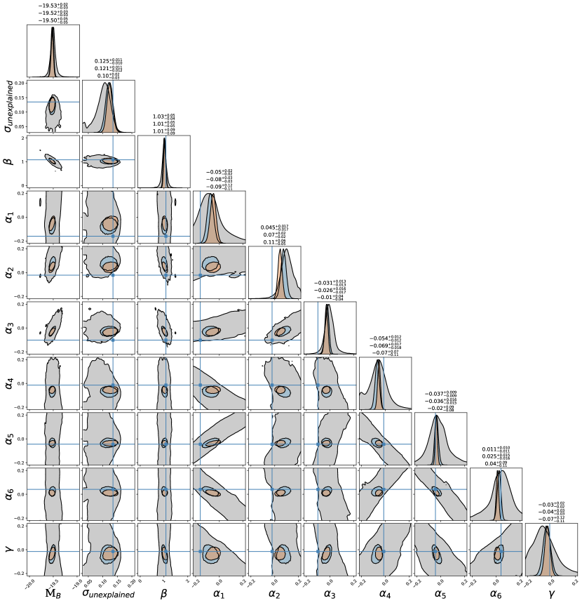
Figure 4: Same as Figure 3, but using SNEMO7 to fit the light curves. Three different uncertainty models are shown: no uncertainty model (orange, top numbers), 1% of peak uncertainty floor (blue, middle numbers), and a 2% uncertainty (gray, bottom numbers). For several parameters, there is not enough statistical significance to distinguish the standardization parameters ($\alpha_{i}$, $\gamma$) from zero with any significance, this is especially true for the 2% uncertainty floor. Nevertheless, the 2% uncertainty floor does reveal many tight correlations between the parameters (e.g. $\alpha_{1}$–$\alpha_{5}$ & $\alpha_{4}$–$\alpha_{6}$) implying that with a reduction of one or two parameters, the others would likely be determinable. The blue lines for $\sigma_{\rm unexplained}$ and $\gamma$ are from the SALT2 fits of the same data set. Whereas, the other lines, $\alpha_{i}$ and $\beta$, are the values presented in Saunders et al. (2018).

There are a few things that stand out from these results. First, in Table 3, we see that the outlier percentage typically ranges from 1.5% to 3.2%. UNITY1.2 probabilistically separates these into an outlier population, where they do not affect the inlier population variables: ${\rm M}_{\rm B}$, $\sigma_{\rm unexplained}$, $\alpha_{i}$, $\beta$, and $\gamma$. Next, the intrinsic scatter starts at $0.125\pm 0.011~{}\text{mag}$, slightly smaller than that of SALT2, and decreases if we raise the uncertainty floor to 2%. Finally, as the size of the uncertainty model increases, the sample size decreases and as expected the uncertainty in the standardization parameters increase.

Table 2: Parameter estimation results from UNITY1.2 for SN Ia that passed SNEMO2 quality cuts.

	SALT2	SNEMO2
% Error Model		0	1	2
Data set size	867	885	886	881
MB	$-19.193^{+0.006}_{-0.006}$	$-19.444^{+0.011}_{-0.010}$	$-19.452^{+0.011}_{-0.011}$	$-19.455^{+0.011}_{-0.011}$
$\sigma_{\rm unexplained}$	$0.116^{+0.006}_{-0.005}$	$0.129^{+0.007}_{-0.007}$	$0.117^{+0.007}_{-0.007}$	$0.102^{+0.008}_{-0.008}$
$\beta$	$2.85^{+0.06}_{-0.07}$	$0.88^{+0.03}_{-0.04}$	$0.91^{+0.03}_{-0.04}$	$0.91^{+0.04}_{-0.03}$
$\alpha_{1}$	$-0.126^{+0.006}_{-0.006}$	$0.044^{+0.007}_{-0.007}$	$0.045^{+0.007}_{-0.007}$	$0.045^{+0.008}_{-0.008}$
$\gamma$	$-0.043^{+0.010}_{-0.010}$	$-0.039^{+0.014}_{-0.014}$	$-0.042^{+0.014}_{-0.014}$	$-0.039^{+0.014}_{-0.015}$
No. of outliers	15 (1.7%)	21 (2.4%)	20 (2.3%)	26 (3.0%)

Note. — The SN Ia used in the SALT2 analysis are the ones that passed the $\sigma_{i}\leq 2$ for SNEMO2 with no error model and were successfully fit with SALT2. The “No. of outliers” is reported both as an absolute number and a percentage of the data set.

Table 3: Parameter estimation results from UNITY1.2 for SN Ia that passed SNEMO7 quality cuts.

	SALT2			Saunders et al. (2018)	SNEMO7
% Error Model					0	1	2
Data set size	240	194	126	133	240	194	126
MB	$-19.197^{+0.011}_{-0.011}$	$-19.196^{+0.012}_{-0.012}$	$-19.188^{+0.017}_{-0.017}$	$\cdots$	$-19.53^{+0.02}_{-0.03}$	$-19.52^{+0.03}_{-0.03}$	$-19.50^{+0.05}_{-0.05}$
$\sigma_{\rm unexplained}$	$0.135^{+0.009}_{-0.009}$	$0.131^{+0.011}_{-0.011}$	$0.141^{+0.015}_{-0.015}$	$\cdots$	$0.125^{+0.011}_{-0.010}$	$0.121^{+0.011}_{-0.012}$	$0.10^{+0.02}_{-0.03}$
$\beta$	$3.02^{+0.10}_{-0.10}$	$2.84^{+0.10}_{-0.10}$	$2.96^{+0.14}_{-0.14}$	$1.08\pm 0.04$	$1.03^{+0.05}_{-0.04}$	$1.01^{+0.05}_{-0.05}$	$1.01^{+0.09}_{-0.09}$
$\alpha_{1}$	$-0.125^{+0.010}_{-0.010}$	$-0.129^{+0.012}_{-0.012}$	$-0.122^{+0.017}_{-0.017}$	$0.16\pm 0.03$	$-0.05^{+0.02}_{-0.02}$	$-0.08^{+0.03}_{-0.03}$	$-0.09^{+0.12}_{-0.11}$
$\alpha_{2}$	$\cdots$	$\cdots$	$\cdots$	$0.02\pm 0.03$	$0.045^{+0.017}_{-0.017}$	$0.07^{+0.02}_{-0.02}$	$0.11^{+0.06}_{-0.05}$
$\alpha_{3}$	$\cdots$	$\cdots$	$\cdots$	$0.103\pm 0.017$	$-0.031^{+0.013}_{-0.013}$	$-0.026^{+0.016}_{-0.017}$	$-0.01^{+0.04}_{-0.04}$
$\alpha_{4}$	$\cdots$	$\cdots$	$\cdots$	$0.01\pm 0.02$	$-0.054^{+0.012}_{-0.012}$	$-0.069^{+0.017}_{-0.018}$	$-0.07^{+0.07}_{-0.11}$
$\alpha_{5}$	$\cdots$	$\cdots$	$\cdots$	$0.045\pm 0.009$	$-0.037^{+0.009}_{-0.009}$	$-0.036^{+0.016}_{-0.015}$	$-0.02^{+0.09}_{-0.08}$
$\alpha_{6}$	$\cdots$	$\cdots$	$\cdots$	$-0.041\pm 0.017$	$0.011^{+0.010}_{-0.011}$	$0.025^{+0.015}_{-0.016}$	$0.04^{+0.09}_{-0.11}$
$\gamma$	$-0.01^{+0.02}_{-0.02}$	$-0.03^{+0.03}_{-0.03}$	$-0.04^{+0.05}_{-0.05}$	$\cdots$	$-0.03^{+0.02}_{-0.02}$	$-0.04^{+0.03}_{-0.03}$	$-0.07^{+0.12}_{-0.11}$
No. of outliers	4 (1.7%)	4 (2.1%)	4 (3.2%)	$\cdots$	7 (2.9%)	3 (1.5%)	4 (3.2%)

Note. — The SN Ia used in the SALT2 analysis are the ones that passed each of the SNEMO7 analyses, respectively. The “No. of outliers” is reported both as an absolute number and a percent of the data set.

3.2.1 Are the standardization coefficients consistent between data sets?

Table 3 shows the estimated standardization coefficients after applying various data quality cuts. Taking the data with no uncertainty model added, we determine that they differ at $\sim 2\sigma$ with the original estimates produced when using the SNfactory data set (Saunders et al., 2018, and forthcoming erratum). When evaluating seven parameters, it is expected to see some variability. In this analysis, $\alpha_{3}$ differs at $>3\sigma$ from the SNfactory numbers. Having only one parameter reach this level of disagreement is expected in about 2% of analysis, or $\gtrsim 2\sigma$. Including a non-zero mass standardization does slightly shift the central values of the other standardization coefficients, but not by the scale of the variation described above. The correlations between $\gamma$ and each $\alpha$, seen in Figure 4, are not large enough to cause a drastic shift in any of the standardization coefficients. Furthermore, these values can shift by over $1\sigma$ (e.g. $\alpha_{1}$) with the addition of a 1% uncertainty model. Our results show that the standardization coefficients for SNEMO7 show only mild variation between data sets.

3.2.2 How many standardization coefficients are distinguishable from zero?

Using SNEMO7 with no model uncertainties, most coefficients can be distinguished from zero at $>2\sigma$, with $\alpha_{4}$ distinguishable from 0 at greater than $4\sigma$. A 1% uncertainty model has similar results. However with a 2% uncertainty model, UNITY1.2 is unable to distinguish the SNEMO7 standardization components from zero (except for $\alpha_{2}$). This is likely due to a combination of data set size and the quality of the light curves themselves. Assuming SNEMO7 has an uncertainty model below $\sim$ 2%, each light-curve parameter will have a non-zero standardization coefficient.

3.2.3 What are the correlations between the coefficients?

The 2% uncertainty model does reveal strong correlations between the parameters. These strong correlations the constrainability of the standardization parameters would dramatically improve if one or two of these parameters were fixed or known. A lower dimensional model (like SNEMO6 or SNEMO5) would have an effect similar to “fixing” one or two of these parameters to zero. However, since a five parameter EMFA model is not simply the first five parameters of a seven parameter EMFA model, SNEMO5 would require a full retraining rather than truncation of SNEMO7.

When looking at spectral time series data, SNEMO7 appears to be a viable photometric light-curve fitter, but these strong correlations imply that not all of the eigenvectors are constrainable with today’s light curves. Since a much higher percentage of the higher cadence CSP SN Ia passed quality cuts, we know that the quality of the observed light curves plays a role in the ability of SNEMO7 to be used with photometric data. Additionally, the eigenvectors that could be obtained from light curves are not necessarily the same, nor in the same order, as those obtained from spectral time series (like the SNEMO eigenvectors). Similar to the work of Kim et al. (2013), the SNEMO eigenvectors manifested in light curves should be investigated and perhaps a new model generated that prioritizes the information available in the light curves.

3.2.4 Does SNEMO7 reduce unexplained and systematic variations in standardization?

The final two questions deal with the uniformity of the standardization. Using the light curves with no additional error model, the unexplained intrinsic scatter ($\sigma_{\rm unexplained}$) moderately decreased from $0.135\pm 0.009~{}\text{mag}$ with SALT2 to $0.125\pm 0.011~{}\text{mag}$, . We found that with a 2% uncertainty model, the unexplained intrinsic scatter decreased from $0.141\pm 0.015~{}\text{mag}$ for SALT2 to $0.10\pm 0.03~{}\text{mag}$. Because this is a more direct comparison to the $\sigma_{\rm unexplained}$ of SALT2, as both methods use some uncertainty model, we conclude that SNEMO7 is capable of decreasing the unexplained intrinsic scatter on the Hubble-Lemaître diagram. With regard to the reduction of unexplained variation or systematic limits of standardization, SNEMO7 shows only slightly significant deviations from SNEMO2 or SALT2.

We also found that there was no apparent decrease in the host galaxy stellar mass dependence. For the SNEMO7 data set, SALT2 only sees a non-zero mass dependence at $0.5\sigma$, whereas, with no uncertainty model the mass dependence of SNEMO7 was measured to have a $1.5\sigma$ non-zero statistical significance. As discussed in Section 2.3, this is not a removal of a host galaxy mass correlation, but more likely an inflation of its uncertainty due to the small sample size.

4 Impacts on Systematics Dominated Cosmology

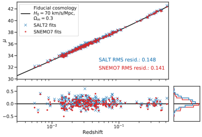
Figure 5:

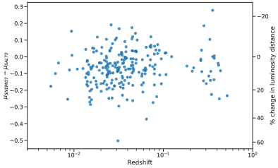
Figure 6:

5 Conclusion

SNEMO is a family of SN Ia models trained on the spectrophotometric time series data of SNfactory. One of the many potential uses of these models is to standardise SNe Ia for cosmological measurements. In testing that use case with current data sets, we are able to consistently determine the standardisation parameters for SNEMO7, but tight correlations between the parameters implies that with a reduction of one or two , the other parameters should be much easier to constrain. This means that SNEMO5 or SNEMO6 would be good candidates for a new light-curve fitter with a goal of cosmological standardisation of current data sets.

Once we add a modest uncertainty model — similar to the one present in SALT2 — SNEMO2 and SNEMO7 have a reduction in $\sigma_{\rm unexplained}$ indicating that SNEMO explains more of the natural variation of SN Ia. On the other hand, there is no statistically significant reduction in a stellar mass dependence, implying that adding more linearly standardized light-curve parameters, with SNEMO7, would be susceptible to a similar systematic uncertainty floor as SALT2 and that we may be approaching the limits of Tripp-standardization. This perhaps motivates consideration of non-linear relationships.

SNEMO7 describes more of the intrinsic variation of SN Ia as seen in the reduction of the RMS in Figure 5. These unaccounted for variations have been shown to be responsible for a significant fraction of the unexplained intrinsic dispersion seen in SALT2 analyses (Fakhouri et al., 2015). Therefore, there is a danger that if one leaves these differences unaccounted for, SN Ia sets at different redshifts could systematically favor one side or the other of this unexplained intrinsic dispersion, thus introducing a systematic in any cosmological measurement. If we cannot constrain models that explain more of this intrinsic dispersion, we risk being unable to reach the level of precision planned for future cosmological surveys.

The family of SNEMO models are not intrinsically unconstrainable, as SNEMO2 can easily be constrained with present data. On the other hand, only the highest quality among currently available light curves could be fit by SNEMO7, and the resulting data set is dominated by SN Ia observed by CSP. Therefore, it is likely that upcoming large surveys, such as LSST and WFIRST, will want to specify CSP-like signal-to-noise, time sampling, and rest-frame wavelength coverage for a reasonable fraction of their supernova photometry. Such light curves could be fit by SNEMO7 and gain the benefit of better constraints on the SN Ia differences. It is also possible that one or more spectra might be needed. Further work is essential in order to properly understand the data requirements needed for high quality and cosmologically useful fits of light curves with SNEMO7. Part of this work is already in preparation but additional SNEMO models with fewer light-curve shape parameters should also be investigated. This would include an investigation into possible information loss or reordering of eigenvectors by going from the spectrophotmetric time series data to light-curve data.

We have presented a first look at SNEMO7’s ability to be a replacement for SALT2 in cosmological analyses. since neither the philosophy behind SNEMO nor photometry-only data sets are roadblocks to its future use.

Appendix A Effect of Signal to Noise Cuts

The $\sigma_{i}\leq 2$ cut is a subjective choice and therefore could have a noticeable effect on the results presented. As such, we reran UNITY1.2 on data sets with cuts applied at $\sigma_{i}\leq 1$. These results are listed in Table LABEL:tab:snemo7sigma1results. While using the 1% uncertainty model, Figure 7 shows the effects of changing the value of the $\sigma_{i}$ cut.

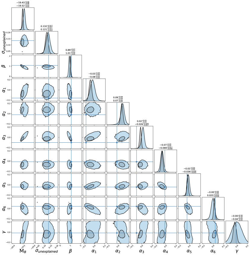
Figure 7: The same as Figure 4 but showing the effect of changing $\sigma_{i}$. These data sets use a 1% uncertainty model and use quality cuts of $\sigma_{i}\leq 1$ (blue) and $\sigma_{i}\leq 2$ (gray, blue in Figure 4). Changing the signal to noise cut has no significant ($<2\sigma$) effect on the UNITY1.2 parameter estimation. This increase in uncertainty is expected for the decrease in sample size.

As expected, the effect of changing from a quality cut of $\sigma_{i}\leq 2$ are slight and statistically insignificant. The uncertainty on the parameters are inflated when moving from $\sigma_{i}\leq 2$ to $\sigma_{i}\leq 1$ but this is largely due to the decrease in sample size, from 194 SN Ia to 90 respectively, rather than the actual value of $\sigma_{i}$. Ultimately, the ability to standardize SNEMO7 light-curve fits shows no significant dependence on reasonable light-curve fit quality cuts.

Table 4:

	SNEMO7
% Error Model	0	1	2
Data set size	157	90	39
MB	$-19.52^{+0.04}_{-0.05}$	$-19.43^{+0.06}_{-0.06}$	$-19.4^{+0.2}_{-0.3}$
$\sigma_{\rm unexplained}$	$0.135^{+0.015}_{-0.014}$	$0.132^{+0.017}_{-0.017}$	$0.06^{+0.04}_{-0.03}$
$\beta$	$1.05^{+0.07}_{-0.06}$	$0.89^{+0.07}_{-0.07}$	$0.71^{+0.17}_{-0.17}$
$\alpha_{1}$	$-0.05^{+0.03}_{-0.04}$	$-0.03^{+0.05}_{-0.05}$	$0.18^{+0.07}_{-0.07}$
$\alpha_{2}$	$0.04^{+0.02}_{-0.03}$	$0.09^{+0.04}_{-0.04}$	$0.18^{+0.05}_{-0.05}$
$\alpha_{3}$	$-0.03^{+0.02}_{-0.02}$	$0.02^{+0.03}_{-0.03}$	$0.08^{+0.05}_{-0.05}$
$\alpha_{4}$	$-0.055^{+0.017}_{-0.017}$	$-0.07^{+0.03}_{-0.03}$	$-0.17^{+0.05}_{-0.06}$
$\alpha_{5}$	$-0.040^{+0.014}_{-0.013}$	$-0.02^{+0.03}_{-0.03}$	$0.07^{+0.04}_{-0.04}$
$\alpha_{6}$	$0.014^{+0.016}_{-0.017}$	$-0.004^{+0.03}_{-0.04}$	$-0.10^{+0.06}_{-0.06}$
$\gamma$	$-0.06^{+0.05}_{-0.05}$	$-0.001^{+0.10}_{-0.10}$	$-0.02^{+0.9}_{-1.1}$
No. of outliers	6 (3.8%)	1 (1.1%)	8 (21%)

Note. — The “No. of outliers” is reported both as an absolute number and a percent of the data set.

References

- Aldering et al. (2002) Aldering, G., Adam, G., Antilogus, P., et al. 2002, in (International Society for Optics and Photonics), 61
- Astropy Collaboration (2013) Astropy Collaboration. 2013, A&A, 558, 33
- Betoule et al. (2014) Betoule, M., Kessler, R., Guy, J., et al. 2014, Astronomy & Astrophysics, 568, A22
- Bohlin et al. (2014) Bohlin, R. C., Gordon, K. D., & Tremblay, P.-E. 2014, Publications of the Astronomical Society of the Pacific, 000
- Branch et al. (2006) Branch, D., Dang, L. C., Hall, N., et al. 2006, Publications of the Astronomical Society of the Pacific, 118, 560
- Burns et al. (2011) Burns, C. R., Stritzinger, M., Phillips, M. M., et al. 2011, The Astronomical Journal, 141, 19
- Burns et al. (2018) Burns, C. R., Parent, E., Phillips, M. M., et al. 2018, ApJ, 869, 56
- Carpenter et al. (2017) Carpenter, B., Gelman, A., Hoffman, M. D., et al. 2017, Journal of Statistical Software, 76, 1
- Childress et al. (2013) Childress, M., Aldering, G., Antilogus, P., et al. 2013, ApJ, 770, 108
- Childress et al. (2014) Childress, M. J., Wolf, C., & Zahid, H. J. 2014, MNRAS, 445, 1898
- DES Collaboration et al. (2019) DES Collaboration, Abbott, T. M. C., Allam, S., et al. 2019, ApJ, 872, L30
- Fakhouri et al. (2015) Fakhouri, H. K., Boone, K., Aldering, G., et al. 2015, ApJ, 815, 58
- Fitzpatrick & Massa (2007) Fitzpatrick, E. L., & Massa, D. 2007, ApJ, 663, 320
- Foley & Kasen (2011) Foley, R. J., & Kasen, D. 2011, ApJ, 729, 55
- Foley et al. (2018) Foley, R. J., Scolnic, D., Rest, A., et al. 2018, MNRAS, 475, 193
- Foreman-Mackey (2016) Foreman-Mackey, D. 2016, The Journal of Open Source Software, 24, doi:10.21105/joss.00024
- Foreman-Mackey et al. (2012) Foreman-Mackey, D., Hogg, D. W., Lang, D., & Goodman, J. 2012, arXiv:1202.3665
- Gupta et al. (2011) Gupta, R. R., D’Andrea, C. B., Sako, M., et al. 2011, ApJ, 740, 92
- Guy et al. (2005) Guy, J., Astier, P., Nobili, S., Regnault, N., & Pain, R. 2005, Astronomy & Astrophysics, 443, 781
- Guy et al. (2007) Guy, J., Astier, P., Baumont, S., et al. 2007, A&A, 466, 11
- Guy et al. (2010) Guy, J., Sullivan, M., Conley, A., et al. 2010, A&A, 523, A7
- Hamuy et al. (1996) Hamuy, M., Phillips, M. M., Suntzeff, N. B., et al. 1996, AJ, 112, 2408
- Hayden et al. (2019) Hayden, B., Rubin, D., & Strovink, M. 2019, ApJ, 871, 219
- Hayden et al. (2013) Hayden, B. T., Gupta, R. R., Garnavich, P. M., et al. 2013, ApJ, 764, 191
- Hicken et al. (2009) Hicken, M., Wood-Vasey, W. M., Blondin, S., et al. 2009, ApJ, 700, 1097
- Hicken et al. (2012) Hicken, M., Challis, P., Kirshner, R. P., et al. 2012, astro-ph.C
- Hounsell et al. (2018) Hounsell, R., Scolnic, D., Foley, R. J., et al. 2018, ApJ, 867, 23
- Hunter (2007) Hunter, J. D. 2007, Computing in Science & Engineering, 9, 90
- Jha et al. (2007) Jha, S., Riess, A. G., & Kirshner, R. P. 2007, ApJ, 659, 122
- Jha et al. (2006) Jha, S., Kirshner, R. P., Challis, P., et al. 2006, ApJ, 131, 527
- Jones et al. (2001) Jones, E., Oliphant, T., Peterson, P., et al. 2001, SciPy: Open Source Scientific Tools for Python
- Kelly et al. (2010) Kelly, P. L., Hicken, M., Burke, D. L., Mandel, K. S., & Kirshner, R. P. 2010, ApJ, 715, 743
- Kessler & Scolnic (2017) Kessler, R., & Scolnic, D. 2017, ApJ, 836, 56
- Kessler et al. (2009) Kessler, R., Bernstein, J. P., Cinabro, D., et al. 2009, PASP, 121, 1028
- Kim et al. (2013) Kim, A. G., Thomas, R. C., Aldering, G., et al. 2013, ApJ, 766, 84
- Kim et al. (2014) Kim, A. G., Aldering, G., Antilogus, P., et al. 2014, The Astrophysical Journal, 784, 51
- Krisciunas et al. (2017) Krisciunas, K., Contreras, C., Burns, C. R., et al. 2017, ApJ, 154, 211
- Kunz et al. (2007) Kunz, M., Bassett, B. A., & Hlozek, R. A. 2007, Phys. Rev. D, 75, 103508
- Lampeitl et al. (2010) Lampeitl, H., Smith, M., Nichol, R. C., et al. 2010, ApJ, 722, 566
- LSST Science Collaboration (2009) LSST Science Collaboration. 2009, arXiv:0912.0201
- McKinney (2010) McKinney, W. 2010, Data Structures for Statistical Computing in Python
- Moreno-Raya et al. (2018) Moreno-Raya, M. E., Galbany, L., López-Sánchez, Á. R., et al. 2018, Monthly Notices of the Royal Astronomical Society, 476, 307
- Mosher et al. (2014) Mosher, J., Guy, J., Kessler, R., et al. 2014, The Astrophysical Journal, 793, 16
- Perlmutter et al. (1997) Perlmutter, S., Gabi, S., Goldhaber, G., et al. 1997, ApJ, 483, 565
- Perlmutter et al. (1999) Perlmutter, S., Aldering, G., Goldhaber, G., et al. 1999, ApJ, 517, 565
- Phillips (1993) Phillips, M. M. 1993, ApJ, 413, L105
- Phillips et al. (1999) Phillips, M. M., Lira, P., Suntzeff, N. B., et al. 1999, The Astronomical Journal, 118, 1766
- Pierel et al. (2018) Pierel, J. D. R., Rodney, S., Avelino, A., et al. 2018, PASP, 130, 114504
- Pskovskii (1977) Pskovskii, Y. P. 1977, Soviet Astronomy, 675
- Riess et al. (1999) Riess, A. G., Kirshner, R. P., Schmidt, B. P., et al. 1999, ApJ, 117, 707
- Riess et al. (1996) Riess, A. G., Press, W. H., & Kirshner, R. P. 1996, ApJ, 473, 88
- Riess et al. (1998) Riess, A. G., Filippenko, A. V., Challis, P., et al. 1998, ApJ, 116, 1009
- Riess et al. (2007) Riess, A. G., Strolger, L.-G., Casertano, S., et al. 2007, The Astrophysical Journal, 659, 98
- Rigault et al. (2013) Rigault, M., Copin, Y., Aldering, G., et al. 2013, A&A, 560, A66
- Rigault et al. (2015) Rigault, M., Aldering, G., Kowalski, M., et al. 2015, ApJ, 802, 20
- Rigault et al. (2018) Rigault, M., Brinnel, V., Aldering, G., et al. 2018, arXiv:1806.03849
- Rose et al. (2019) Rose, B. M., Garnavich, P. M., & Berg, M. A. 2019, ApJ, 874, 32
- Rubin (2019) Rubin, D. 2019, ApJ in press, arXiv:1903.10518
- Rubin et al. (2015) Rubin, D., Aldering, G., Barbary, K., et al. 2015, ApJ, 813, 137
- Sako et al. (2014) Sako, M., Bassett, B., Becker, A. C., et al. 2014, arXiv, 1401.3317, arXiv:1401.3317
- Saunders et al. (2018) Saunders, C., Aldering, G., Antilogus, P., et al. 2018, ApJ, 569, 167
- Schlafly & Finkbeiner (2011) Schlafly, E. F., & Finkbeiner, D. P. 2011, The Astrophysical Journal, 737, 103
- Scolnic et al. (2018) Scolnic, D. M., Jones, D. O., Rest, A., et al. 2018, ApJ, 859, 101
- Spergel et al. (2015) Spergel, D., Gehrels, N., Baltay, C., et al. 2015, arXiv:1503.03757
- Sullivan et al. (2010) Sullivan, M., Conley, A., Howell, D. A., et al. 2010, MNRAS, 406, 782
- Tripp (1998) Tripp, R. 1998, A&A, 331, 815
- Uddin et al. (2017) Uddin, S. A., Mould, J., Lidman, C., Ruhlmann-Kleider, V., & Zhang, B. R. 2017, ApJ, 848, 56
- van der Walt et al. (2011) van der Walt, S., Colbert, S. C., & Varoquaux, G. 2011, Computing in Science & Engineering, 13, 22