Proca tubes with the flux of the longitudinal chromoelectric field
and the energy flux/momentum density

Abstract

We consider non-Abelian SU(3) Proca theory with a Higgs scalar field included. Cylindrically symmetric solutions describing classical tubes either with the flux of a longitudinal electric field or with the energy flux (and hence with nonzero momentum density) are obtained. It is shown that, in quantum Proca theory, there can exist tubes both with the flux of the longitudinal electric field and with the energy flux/momentum density simultaneously. An imaginary particle – Proca proton – in which ‘quarks’ are connected by tubes with nonzero momentum density is considered. It is shown that this results in the appearance of the angular momentum related to the presence of the non-Abelian electric and magnetic fields in the tube, and this angular momentum is a part of the Proca proton spin.

I Introduction

In recent years there is a growing interest in modelling systems containing various massive vector fields. Such fields are described within gauge Proca theories (both Abelian and non-Abelian ones) where the gauge invariance is violated explicitly by introducing a mass term. Being the generalization of Maxwell’s theory, Proca theory permits one to take into account various effects related to the possible presence of the mass of vector particles. At the present time, Proca fields are used in different aspects: in constructing models of black holes Heisenberg:2017xda , hypothetical Proca stars Brito:2015pxa ; Herdeiro:2017fhv ; Dzhunushaliev:2019kiy ; Herdeiro:2019mbz , in studying the generalized Proca theories Heisenberg:2014rta ; Allys:2015sht ; Heisenberg:2016eld and solitons Babichev:2017rti , in describing the massive spin-1 $Z^{0}$ and $W^{\pm}$ bosons in the standard model Lawrie2002 , in considering various effects related to the possible presence of the rest mass of a photon Tu:2005ge , and within dark matter physics Pospelov:2008jd .

When considering configurations containing Proca fields, the main efforts have been focused on studying spherically symmetric solutions. However, a consideration of cylindrically symmetric systems seems to be of interest as well. In particular, cylindrically symmetric localized regular solutions (the so-called ‘Proca Q tubes’) have been found in Ref. Brihaye:2016pld .

The next natural step in this direction is to generalize systems containing Proca fields by including extra fields in them. For example, for a spherically symmetric case, in Proca theories involving some extra fields, there can occur topologically trivial monopoles with an exponentially decaying radial magnetic field Dzhunushaliev:2019ham . In the present paper we show that, in non-Abelian Proca theories containing a Higgs scalar field, there exist cylindrically symmetric solutions describing tubes filled with color electric and magnetic fields. The distinctive feature of these tubes is that they can contain either the flux of the longitudinal electric field sourced by ‘quarks’ located at $\pm\infty$ or the energy flux associated with the presence of nonzero Poynting vector (and hence a nonzero momentum density). [Henceforth, by ‘quarks’ (in quotation marks) we mean the sources of non-Abelian Proca fields, analogous to what is done in quantum chromodynamics for Yang-Mills fields and real quarks.]

The paper is organized as follows. In Sec. II, we write down the general field equations for the non-Abelian-Proca-Higgs theory. In Sec. III, we obtain cylindrically symmetric solutions to the equations of Sec. II describing tubes which contain either the flux of the electric field or the energy flux (and hence the momentum density). In Sec. IV, we present some qualitative arguments in favor of the fact that, in quantum Proca theory, there can exist tubes containing simultaneously both the flux of the longitudinal electric field and the energy flux/momemtum density. In Sec. V, we show that tubes with nonzero momentum density connecting three ‘quarks’ in a Proca proton do create the angular momentum that is a part of the Proca proton spin. Finally, in Sec. VI, we summarize the results obtained in the present paper.

II Non-Abelian-Proca-Higgs theory

The Lagrangian describing a system consisting of a non-Abelian SU(3) Proca field $A^{a}_{\mu}$ interacting with nonlinear scalar field $\phi$ can be taken in the form (hereafter, we work in units such that $c=\hbar=1$)

$$\mathcal{L}=-\frac{1}{4}F^{a}_{\mu\nu}F^{a\mu\nu}-\frac{\left(\mu^{2}\right)^{ab,\mu}_{\phantom{ab,}\nu}}{2}A^{a}_{\mu}A^{b\nu}+\frac{1}{2}\partial_{\mu}\phi\partial^{\mu}\phi+\frac{\lambda}{2}\phi^{2}A^{a}_{\mu}A^{a\mu}-\frac{\Lambda}{4}\left(\phi^{2}-M^{2}\right)^{2}.$$ (1)

Here $F^{a}_{\mu\nu}=\partial_{\mu}A^{a}_{\nu}-\partial_{\nu}A^{a}_{\mu}+gf_{abc}A^{b}_{\mu}A^{c}_{\nu}$ is the field strength tensor for the Proca field, where $f_{abc}$ are the SU(3) structure constants, $g$ is the coupling constant, $a,b,c=1,2,\dots,8$ are color indices, $\mu,\nu=0,1,2,3$ are spacetime indices. The Lagrangian (1) also contains the arbitrary constants $M,\lambda,\Lambda$ and the Proca field mass matrix $\left(\mu^{2}\right)^{ab,\mu}_{\phantom{ab,}\nu}$.

Using (1), the corresponding field equations can be written in the form

$$D_{\nu}F^{a\mu\nu}-\lambda\phi^{2}A^{a\mu} = -\left(\mu^{2}\right)^{ab,\mu}_{\phantom{ab,}\nu}A^{b\nu},$$ (2)

$$\Box\phi = \lambda A^{a}_{\mu}A^{a\mu}\phi+\Lambda\phi\left(M^{2}-\phi^{2}\right),$$ (3)

and the energy density is

$$\begin{split}\varepsilon=&\frac{1}{2}\left(E^{a}_{i}\right)^{2}+\frac{1}{2}\left(H^{a}_{i}\right)^{2}-\left[\left(\mu^{2}\right)^{ab,\alpha}_{\phantom{ab,}0}A^{a}_{\alpha}A^{b}_{0}-\frac{1}{2}\left(\mu^{2}\right)^{ab,\alpha}_{\phantom{ab,}\beta}A^{a}_{\alpha}A^{b\beta}\right]+\frac{1}{2}\left(\partial_{t}\phi\right)^{2}+\frac{1}{2}\left(\nabla\phi\right)^{2}\\ &+\lambda\phi^{2}\left[\left(A^{a}_{0}\right)^{2}-\frac{1}{2}A^{a}_{\alpha}A^{a\alpha}\right]+\frac{\Lambda}{4}\left(\phi^{2}-M^{2}\right)^{2},\end{split}$$ (4)

where $i=1,2,3$ and $E^{a}_{i}$ and $H^{a}_{i}$ are the components of the electric and magnetic field strengths, respectively.

III Proca flux tubes with the energy flux (momentum density) and the flux of the electric field

The focus of this section is on obtaining and solving equations for two different types of flux tubes containing either the flux of the electric field or the energy flux (and hence the momentum density).

III.1 Proca tube with the flux of the longitudinal electric field

To obtain a tube filled with a longitudinal color electric field, we choose the Ansätze

$$A^{2}_{t}=\frac{h(\rho)}{g},\;A^{5}_{z}=\frac{v(\rho)}{g},\;A^{7}_{\varphi}=\frac{\rho w(\rho)}{g},\;\phi=\phi(\rho),$$ (5)

where $\rho,z,$ and $\varphi$ are cylindrical coordinates. These Ansätze follow from the general cylindrically symmetric Ansatz of Ref. Singleton:1995xc ; Obukhov:1996ry , where it is shown that it is consistent with Yang-Mills-Higgs theory. For such a choice of the SU(3) Proca field potentials, we have the following electric and magnetic field intensities:

$$E^{2}_{\rho} = -\frac{h^{\prime}}{g},\quad E^{5}_{\varphi}=-\frac{\rho hw}{2g},\quad E^{7}_{z}=\frac{hv}{2g},$$

$$H^{2}_{\rho} = -\frac{vw}{2g},\quad H^{5}_{\varphi}=-\frac{\rho v^{\prime}}{g},\quad H^{7}_{z}=\frac{1}{g}\left(w^{\prime}+\frac{w}{\rho}\right).$$

In this case the energy flux is absent, since the Poynting vector is zero,

$$S^{i}=\frac{\epsilon^{ijk}}{\sqrt{\gamma}}E^{a}_{j}H^{a}_{k}=0.$$ (6)

Here, $\epsilon^{ijk}$ is the completely antisymmetric Levi-Civita symbol and $\gamma$ is the determinant of the space metric. For such a tube, the energy density (4) yields

$$\begin{split}g^{2}\varepsilon=&\frac{\left(h^{\prime}\right)^{2}}{2}+\frac{\left(v^{\prime}\right)^{2}}{2}+\frac{1}{2}\left(w^{\prime}+\frac{w}{\rho}\right)^{2}+g^{2}\frac{\left(\phi^{\prime}\right)^{2}}{2}+\frac{1}{8}\left(w^{2}h^{2}+w^{2}v^{2}+h^{2}v^{2}\right)-\frac{\mu_{1}^{2}}{2}h^{2}-\frac{\mu_{2}^{2}}{2}v^{2}-\frac{\mu_{3}^{2}}{2}w^{2}\\ +&\frac{\lambda}{2}\phi^{2}\left(h^{2}+v^{2}+w^{2}\right)+\frac{g^{2}\Lambda}{4}\left(\phi^{2}-M^{2}\right)^{2}\end{split}$$ (7)

with the following components of the Proca field mass matrix: $\mu_{1}^{2}=\left(\mu^{2}\right)^{22,t}_{\phantom{ab,}t}$, $\mu_{2}^{2}=\left(\mu^{2}\right)^{55,z}_{\phantom{ab,}z}$, and $\mu_{3}^{2}=\left(\mu^{2}\right)^{77,\varphi}_{\phantom{ab,}\varphi}$.

Substituting the potentials (5) in Eqs. (2) and (3) and introducing the dimensionless variables $\tilde{\phi}=\phi\sqrt{\lambda}/\phi(0)$, $\tilde{h}=h/\phi(0)$, $\tilde{v}=v/\phi(0)$, $\tilde{w}=w/\phi(0)$, $\tilde{M}=M\sqrt{\lambda}/\phi(0)$, $\tilde{\lambda}=\lambda/g^{2}$, $\tilde{\Lambda}=\Lambda/\lambda$, $\tilde{\mu}_{1,2,3}=\mu_{1,2,3}/\phi(0)$, and $x=\rho\phi(0)$ [here $\phi(0)$ is the central value of the scalar field], we get the following set of equations:

$$\tilde{h}^{\prime\prime}+\frac{\tilde{h}^{\prime}}{x} = h\left(\frac{{\tilde{v}}^{2}}{4}+\frac{\tilde{w}^{2}}{4}+{\tilde{\phi}}^{2}-\tilde{\mu}_{1}^{2}\right),$$ (8)

$$\tilde{v}^{\prime\prime}+\frac{\tilde{v}^{\prime}}{x} = v\left(-\frac{\tilde{h}^{2}}{4}+\frac{\tilde{w}^{2}}{4}+{\tilde{\phi}}^{2}-\tilde{\mu}_{2}^{2}\right),$$ (9)

$$\tilde{w}^{\prime\prime}+\frac{\tilde{w}^{\prime}}{x}-\frac{\tilde{w}}{x^{2}} = \tilde{w}\left(-\frac{\tilde{h}^{2}}{4}+\frac{\tilde{v}^{2}}{4}+{\tilde{\phi}}^{2}-\tilde{\mu}_{3}^{2}\right),$$ (10)

$$\tilde{\phi}^{\prime\prime}+\frac{\tilde{\phi}^{\prime}}{x} = \tilde{\phi}\left[\tilde{\lambda}\left(-\tilde{h}^{2}+\tilde{v}^{2}+\tilde{w}^{2}\right)+\tilde{\Lambda}\left({\tilde{\phi}}^{2}-{\tilde{M}}^{2}\right)\right].$$ (11)

Here, the prime denotes differentiation with respect to the dimensionless radius $x$. We seek a solution to Eqs. (8)-(11) in the vicinity of the origin of coordinates in the form

$$\tilde{h}(x) = \tilde{h}_{0}+\tilde{h}_{2}\frac{x^{2}}{2}+\dots\quad\text{with}\quad\tilde{h}_{2}=\frac{\tilde{h}_{0}}{2}\left(\frac{\tilde{v}_{0}^{2}}{4}+\tilde{\phi}_{0}^{2}-\tilde{\mu}^{2}_{1}\right),$$

$$\tilde{v}(x) = \tilde{v}_{0}+\tilde{v}_{2}\frac{x^{2}}{2}+\dots\quad\text{with}\quad\tilde{v}_{2}=\frac{\tilde{v}_{0}}{2}\left(-\frac{\tilde{h}_{0}^{2}}{4}+\tilde{\phi}_{0}^{2}-\tilde{\mu}^{2}_{2}\right),$$

$$\tilde{w}(x) = \tilde{w}_{1}x+\tilde{w}_{3}\frac{x^{3}}{3!}+\dots\quad\text{with}\quad\tilde{w}_{3}=\frac{3}{4}\tilde{w}_{1}\left(-\frac{\tilde{h}_{0}^{2}}{4}+\frac{\tilde{v}_{0}^{2}}{4}+\tilde{\phi}_{0}^{2}-\tilde{\mu}^{2}_{3}\right),$$

$$\tilde{\phi}(x) = \tilde{\phi}_{0}+\tilde{\phi}_{2}\frac{x^{2}}{2}+\dots\quad\text{with}\quad\tilde{\phi}_{2}=\frac{\tilde{\phi}_{0}}{2}\left[\tilde{\lambda}\left(-\tilde{h}_{0}^{2}+\tilde{v}_{0}^{2}\right)+\tilde{\Lambda}\left({\tilde{\phi}}_{0}^{2}-{\tilde{M}}^{2}\right)\right],$$

where the expansion coefficients $\tilde{h}_{0},\tilde{v}_{0},\tilde{\phi}_{0}$, and $\tilde{w}_{1}$ are arbitrary.

The derivation of solutions to the set of equations (8)-(11) is an eigenvalue problem for the parameters $\tilde{\mu}_{1},\tilde{\mu}_{2},\tilde{\mu}_{3}$, and $\tilde{M}$. The numerical solution describing the behavior of the Proca field potentials and of the corresponding electric and magnetic fields is given in Figs. 4-4.

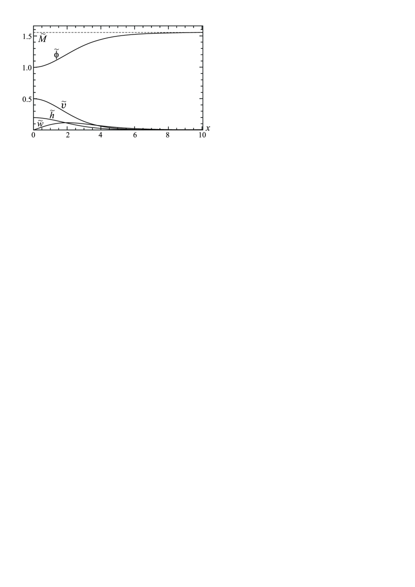
Figure 1: The graphs of the Proca field potentials $\tilde{h}\equiv gA^{2}_{t}/\phi(0)$, $\tilde{v}\equiv gA^{5}_{z}/\phi(0)$, $\tilde{w}\equiv gA^{7}_{\varphi}/x$ and of the scalar field $\tilde{\phi}$ for the following values of the system parameters: $\tilde{\lambda}=2,\tilde{\Lambda}=0.1,\tilde{h}_{0}=0.2,\tilde{v}_{0}=0.5,\tilde{\phi}_{0}=1,\tilde{w}_{1}=0.1,\tilde{M}=1.5520735,\tilde{\mu}_{1}=1.29428281,\tilde{\mu}_{2}=1.28105328,\tilde{\mu}_{3}=1.469883.$

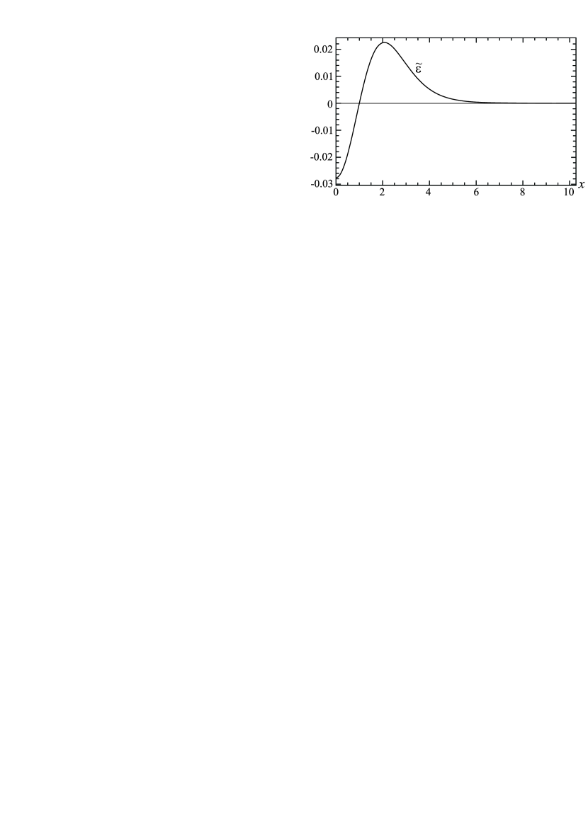
Figure 2: The profile of the dimensionless flux tube energy density $\tilde{\varepsilon}\equiv g^{2}\varepsilon/\phi^{4}(0)$ from Eq. (7) rewritten in terms of the dimensionless variables given before Eq. (8).

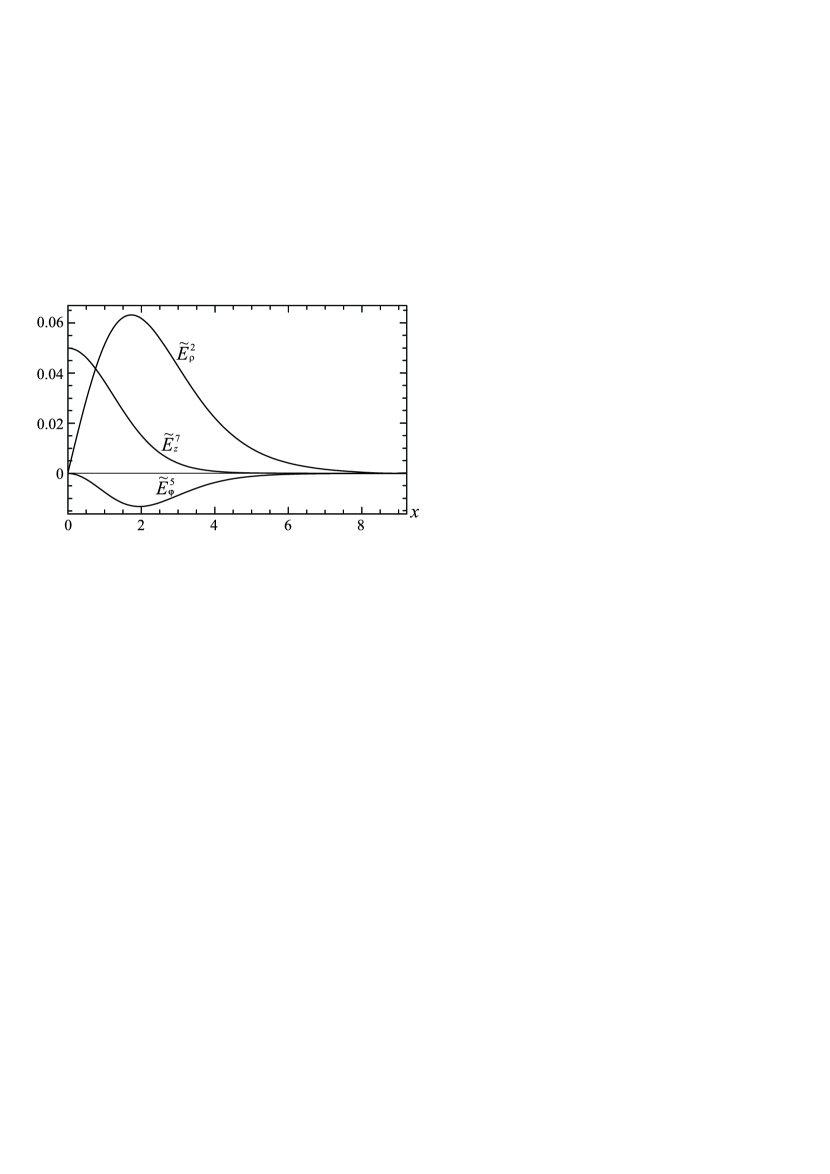
Figure 3: The profiles of the color electric fields $\tilde{E}^{2}_{\rho}\equiv gE^{2}_{\rho}/\phi^{2}(0),\tilde{E}^{5}_{\varphi}\equiv gE^{5}_{\varphi}/\phi(0)$, and $\tilde{E}^{7}_{z}\equiv gE^{7}_{z}/\phi^{2}(0)$.

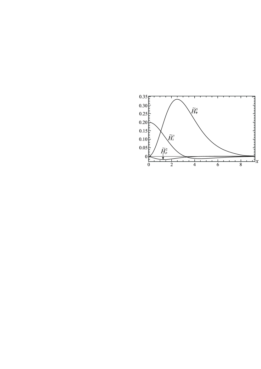
Figure 4: The profiles of the color magnetic fields $\tilde{H}^{2}_{\rho}\equiv gH^{2}_{\rho}/\phi^{2}(0),\tilde{H}^{5}_{\varphi}\equiv gH^{5}_{\varphi}/\phi(0)$, and $\tilde{H}^{7}_{z}\equiv gH^{7}_{z}/\phi^{2}(0)$.

The asymptotic behavior of the functions $\tilde{h},\tilde{v},\tilde{w}$, and $\tilde{\phi}$, which follows from Eqs. (8)-(11), is

$$\tilde{h}(x)\approx\tilde{h}_{\infty}\frac{e^{-x\sqrt{\tilde{M}^{2}-\tilde{\mu}^{2}_{1}}}}{\sqrt{x}},\,\,\tilde{v}(\rho)\approx\tilde{v}_{\infty}\frac{e^{-x\sqrt{\tilde{M}^{2}-\tilde{\mu}^{2}_{2}}}}{\sqrt{x}},\,\,\tilde{w}(\rho)\approx\tilde{w}_{\infty}\frac{e^{-x\sqrt{\tilde{M}^{2}-\tilde{\mu}^{2}_{3}}}}{\sqrt{x}},\,\,\tilde{\phi}\approx\tilde{M}-\tilde{\phi}_{\infty}\frac{e^{-x\sqrt{2\tilde{\Lambda}\tilde{M}^{2}}}}{\sqrt{x}},$$

where $\tilde{h}_{\infty},\tilde{v}_{\infty},\tilde{w}_{\infty}$, and $\tilde{\phi}_{\infty}$ are integration constants.

This flux tube solution has the following characteristics:

• All physical quantities, such as the Proca field potentials, the electric and magnetic field intensities, and the energy density, are finite.

• The tube contains the finite flux of the longitudinal color electric field $E^{7}_{z}$,

  $$\Phi_{z}=2\pi\int\limits_{0}^{\infty}\rho E^{7}_{z}d\rho<\infty.$$

• The tube possesses the finite linear energy density,

  $$\mathcal{E}=2\pi\int\limits_{0}^{\infty}\rho\,\varepsilon(\rho)d\rho<\infty.$$

Thus in this section we have demonstrated that there are cylindrically symmetric solutions within the non-Abelian-Proca-Higgs theory. These solutions describe a tube with the flux of the longitudinal color electric field, and this field is sourced by ‘quarks’/‘antiquarks’ located at $z=\pm\infty$.

III.2 Proca tube with the energy flux/momentum density

Here, we choose the Ansätze

$$A^{5}_{t}=\frac{f(\rho)}{g},\;A^{5}_{z}=\frac{v(\rho)}{g},\;A^{7}_{\varphi}=\frac{\rho w(\rho)}{g},\;\phi=\phi(\rho),$$ (12)

which give the following components of the electric and magnetic field intensities:

$$E^{2}_{\varphi} = \frac{\rho fw}{2g},\quad E^{5}_{\rho}=-\frac{f^{\prime}}{g},\quad$$ (13)

$$H^{2}_{\rho} = -\frac{vw}{2g},\quad H^{5}_{\varphi}=-\frac{\rho v^{\prime}}{g},\quad H^{7}_{z}=\frac{1}{g}\left(w^{\prime}+\frac{w}{\rho}\right).$$ (14)

In this case the Poynting vector (6) is already nonzero [see Eq. (25) below].

Substituting the potentials (12) in Eqs. (2) and (3) and using the dimensionless variables given before Eq. (8), we derive the following equations:

$$\tilde{f}^{\prime\prime}+\frac{\tilde{f}^{\prime}}{x} = \tilde{f}\left(\frac{\tilde{w}^{2}}{4}+{\tilde{\phi}}^{2}-\tilde{\mu}_{1}^{2}\right),$$ (15)

$$\tilde{v}^{\prime\prime}+\frac{\tilde{v}^{\prime}}{x} = \tilde{v}\left(\frac{\tilde{w}^{2}}{4}+{\tilde{\phi}}^{2}-\tilde{\mu}_{2}^{2}\right),$$ (16)

$$\tilde{w}^{\prime\prime}+\frac{\tilde{w}^{\prime}}{x}-\frac{\tilde{w}}{x^{2}} = \tilde{w}\left(-\frac{\tilde{f}^{2}}{4}+\frac{\tilde{v}^{2}}{4}+{\tilde{\phi}}^{2}-\tilde{\mu}_{3}^{2}\right),$$ (17)

$$\tilde{\phi}^{\prime\prime}+\frac{\tilde{\phi}^{\prime}}{x} = \tilde{\phi}\left[\tilde{\lambda}\left(-\tilde{f}^{2}+\tilde{v}^{2}+\tilde{w}^{2}\right)+\tilde{\Lambda}\left({\tilde{\phi}}^{2}-{\tilde{M}}^{2}\right)\right],$$ (18)

where $\tilde{f}=f/\phi(0)$.

This set of equations has a cylindrically symmetric solution describing a tube with nonzero momentum density and energy flux (the Poynting vector). To demonstrate this, let us consider the simplest particular case where $\tilde{f}=\tilde{v}$ and $\tilde{\mu}_{1}=\tilde{\mu}_{2}=\tilde{\mu}$. In this case the set of equations (15)-(18) is split as follows. Eq. (15) takes the form of the Schrödinger equation,

$$-\tilde{f}^{\prime\prime}-\frac{\tilde{f}^{\prime}}{x}+\tilde{f}U_{\tilde{f},\text{eff}}=\tilde{\mu}^{2}\tilde{f},$$ (19)

where the effective potential for the “wave function” $\tilde{f}$ is

$$U_{\tilde{f},\text{eff}}=\frac{\tilde{w}^{2}}{4}+{\tilde{\phi}}^{2}.$$ (20)

In order to ensure a regular solution of this equation, it is necessary that the effective potential would possess a well. In this case Eq. (19) must be solved as an eigenvalue problem for the parameter $\tilde{\mu}^{2}$ with the eigenfunction $\tilde{f}$.

The remaining equations (17) and (18) for the functions $\tilde{w}$ and $\tilde{\phi}$ are then

$$-\tilde{w}^{\prime\prime}-\frac{\tilde{w}^{\prime}}{x}+\tilde{w}U_{\tilde{w},\text{eff}} = \tilde{\mu}_{3}^{2}\tilde{w},$$ (21)

$$\tilde{\phi}^{\prime\prime}+\frac{\tilde{\phi}^{\prime}}{x} = \tilde{\phi}\left[\tilde{\lambda}\tilde{w}^{2}+\tilde{\Lambda}\left({\tilde{\phi}}^{2}-{\tilde{M}}^{2}\right)\right],$$ (22)

and they do not already contain the function $\tilde{f}$. The effective potential, which appears in Eq. (21), is

$$U_{\tilde{w},\text{eff}}=\frac{1}{x^{2}}+{\tilde{\phi}}^{2}.$$ (23)

The equation (21) has the form of the Schrödinger equation with the “wave function” $\tilde{w}$ and with the “energy” $\tilde{\mu}_{3}^{2}$. This means that it will have a regular solution only if the effective potential $U_{\tilde{w},\text{eff}}$ possesses a well. Note also that in the limit $x\to 0$ the effective potential $U_{\tilde{w},\text{eff}}\to 1/x^{2}$, i.e., it is repulsive and hence the “fall of a particle to the centre” is certainly absent.

We will seek regular solutions possessing a finite linear energy density. This means that asymptotically (as $x\rightarrow\infty$) the functions behave as $\tilde{f}(x),\tilde{v}(x),\tilde{w}(x)\rightarrow 0$. Then, taking into account the positiveness of the effective potentials (20) and (23), one can conclude that the function $\tilde{\phi}$ must go to a constant, and Eq. (22) implies that this constant is $\tilde{M}$, i.e., $\tilde{\phi}\rightarrow\tilde{M}\text{ as }x\rightarrow\infty$.

We seek solutions of Eqs. (19), (21), and (22) in the vicinity of the origin of coordinates in the form

$$\tilde{f}(x) = \tilde{f}_{0}+\tilde{f}_{2}\frac{x^{2}}{2}+\dots\quad\text{with}\quad\tilde{f}_{2}=\frac{\tilde{f}_{0}}{2}\left(\tilde{\phi}_{0}^{2}-\tilde{\mu}^{2}\right),$$

$$\tilde{w}(x) = \tilde{w}_{1}x+\tilde{w}_{3}\frac{x^{3}}{3!}+\dots\quad\text{with}\quad\tilde{w}_{3}=\frac{2}{3}\tilde{w}_{1}\left(\tilde{\phi}_{0}^{2}-\tilde{\mu}_{3}^{2}\right),$$

$$\tilde{\phi}(x) = \tilde{\phi}_{0}+\tilde{\phi}_{2}\frac{x^{2}}{2}+\dots\quad\text{with}\quad\tilde{\phi}_{2}=\frac{\tilde{\phi}_{0}}{2}\tilde{\Lambda}\left({\tilde{\phi}}_{0}^{2}-{\tilde{M}}^{2}\right),$$

where the expansion coefficients $\tilde{f}_{0},\tilde{\phi}_{0}$, and $\tilde{w}_{1}$ are arbitrary.

In turn, the asymptotic behavior of the functions is

$$\tilde{f}(x)=\tilde{v}(x)\approx f_{\infty}\frac{e^{-x\sqrt{\tilde{M}^{2}-\tilde{\mu}^{2}}}}{\sqrt{x}},\quad\tilde{w}(x)\approx\tilde{w}_{\infty}\frac{e^{-x\sqrt{\tilde{M}^{2}-\tilde{\mu}^{2}_{3}}}}{\sqrt{x}},\quad\tilde{\phi}\approx\tilde{M}-\tilde{\phi}_{\infty}\frac{e^{-x\sqrt{2\tilde{\Lambda}\tilde{M}^{2}}}}{\sqrt{x}},$$

where $f_{\infty},\tilde{w}_{\infty}$, and $\tilde{\phi}_{\infty}$ are integration constants.

The results of numerical calculations are shown in Figs. 8-8, including the graph for the dimensionless energy density

$$\begin{split}\tilde{\varepsilon}\equiv\frac{g^{2}}{\phi^{4}(0)}\varepsilon=&\frac{\left(\tilde{f}^{\prime}\right)^{2}}{2}+\frac{\left(\tilde{v}^{\prime}\right)^{2}}{2}+\frac{1}{2}\left(\tilde{w}^{\prime}+\frac{\tilde{w}}{x}\right)^{2}+\frac{1}{\tilde{\lambda}}\frac{\left(\tilde{\phi}^{\prime}\right)^{2}}{2}+\frac{\tilde{w}^{2}}{8}\left(\tilde{f}^{2}+\tilde{v}^{2}\right)-\frac{\tilde{\mu}_{1}^{2}}{2}\tilde{f}^{2}-\frac{\tilde{\mu}_{2}^{2}}{2}\tilde{v}^{2}-\frac{\tilde{\mu}_{3}^{2}}{2}\tilde{w}^{2}\\ &+\frac{{\tilde{\phi}}^{2}}{2}\left(\tilde{f}^{2}+\tilde{v}^{2}+\tilde{w}^{2}\right)+\frac{\tilde{\Lambda}}{4\tilde{\lambda}}\left(\tilde{\phi}^{2}-\tilde{M}^{2}\right)^{2}\end{split}$$ (24)

given in Fig. 8.

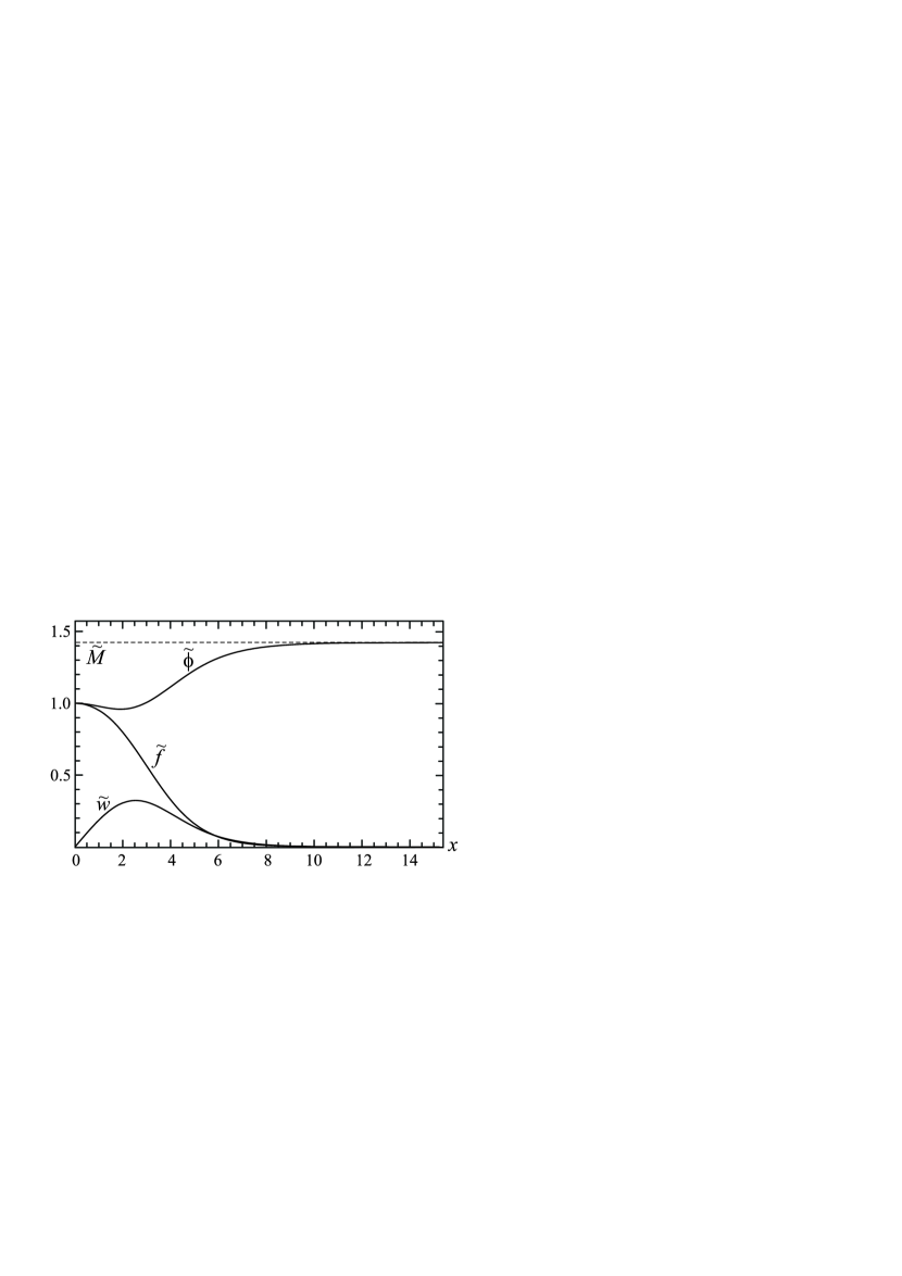
Figure 5: The graphs of the functions $\tilde{w},\tilde{\phi}$, and $\tilde{f}$ for the following values of the system parameters: $\tilde{\lambda}=2,\tilde{\Lambda}=0.1,\tilde{\phi}_{0}=1,\tilde{w}_{1}=0.2,\tilde{f}_{0}=1,\tilde{M}=1.42141,\tilde{\mu}=1.0876563,\tilde{\mu}_{3}=1.206829.$

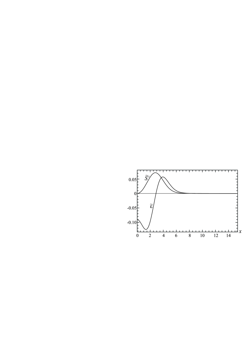
Figure 6: The profiles of the $z$-component of the Poynting vector $\tilde{S}^{z}$ from Eq. (25) and of the energy density $\tilde{\varepsilon}$ from Eq. (24).

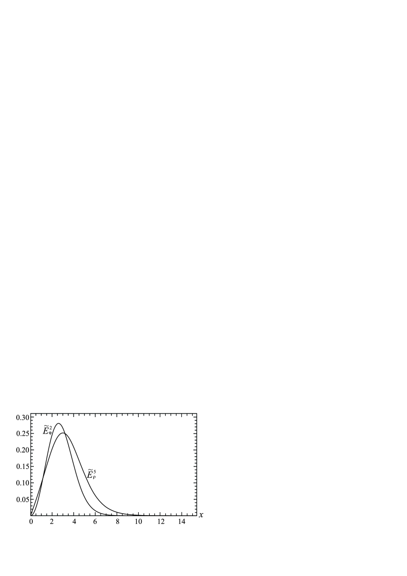
Figure 7: The profiles of the color electric fields $\tilde{E}^{2}_{\varphi}\equiv gE^{2}_{\varphi}/\phi(0)$ and $\tilde{E}^{5}_{\rho}\equiv gE^{5}_{\rho}/\phi^{2}(0)$.

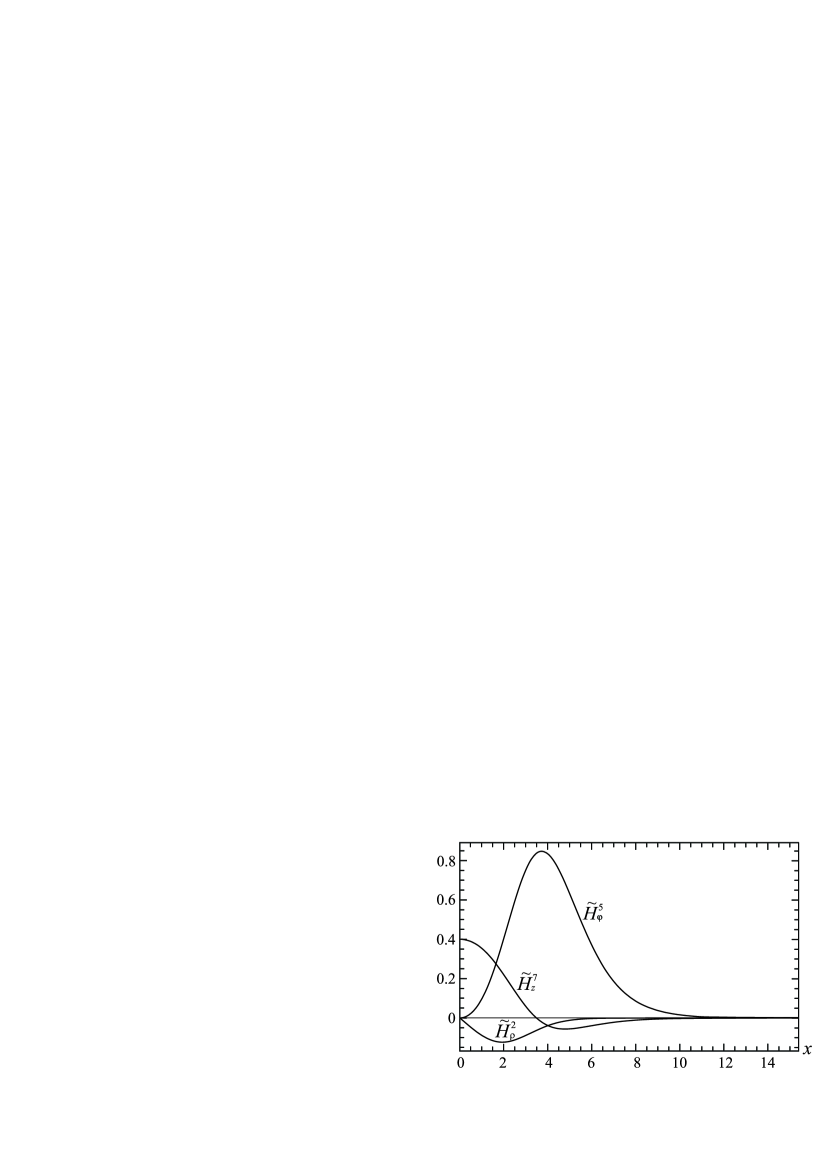
Figure 8: The profiles of the color magnetic fields $\tilde{H}^{2}_{\rho}\equiv gH^{2}_{\rho}/\phi^{2}(0),\tilde{H}^{5}_{\varphi}\equiv gH^{5}_{\varphi}/\phi(0)$, and $\tilde{H}^{7}_{z}\equiv gH^{7}_{z}/\phi^{2}(0)$.

Substitution of the components of electric and magnetic fields (13) and (14) in Eq. (6) yields the following expression for the Poynting vector:

$$S^{z}=\frac{1}{g^{2}}\left(\frac{df}{d\rho}\frac{dv}{d\rho}+\frac{1}{4}fvw^{2}\right)=\frac{\phi^{4}(0)}{g^{2}}\left(\tilde{f}^{\prime}\tilde{v}^{\prime}+\frac{1}{4}\tilde{f}\tilde{v}\tilde{w}^{2}\right)=\frac{\phi^{4}(0)}{g^{2}}\tilde{S}^{z}.$$ (25)

Note the presence of the gradient term $\tilde{f}^{\prime}\tilde{v}^{\prime}$, which is the same as that in Maxwell’s electrodynamics, and of the nonlinear term $\tilde{f}\tilde{v}\tilde{w}^{2}/4$, which appears because the Proca field is non-Abelian.

The flux tube solution obtained in this section has the following characteristics:

• All physical quantities (the Proca electric and magnetic field potentials and intensities, the energy density, the momentum density, and the energy flux) are finite.

• The tube contains a finite linear energy flux directed along the tube and computed as

  $$\Pi^{z}=2\pi\int\limits_{0}^{\infty}\rho S^{z}(\rho)d\rho<\infty.$$

• Since the linear momentum density $\vec{\mathcal{P}}$ is proportional to the linear energy flux, $\vec{\mathcal{P}}=\vec{\Pi}$, the tube also contains the $z$-component of the linear momentum density ${\mathcal{P}}^{z}=\Pi^{z}$.

• In the tube, there is the finite flux of the longitudinal color magnetic field $H^{7}_{z}$,

  $$\Phi_{z}=2\pi\int\limits_{0}^{\infty}\rho H^{7}_{z}d\rho<\infty.$$

• The tube possesses the finite linear energy density,

  $$\mathcal{E}=2\pi\int\limits_{0}^{\infty}\rho\varepsilon(\rho)d\rho<\infty.$$

Thus in this section we have shown that, in the non-Abelian-Proca-Higgs theory, there exist cylindrically symmetric solutions describing a tube possessing the energy flux (and hence the momentum density) between ‘quark’ and ’antiquark’ located at $z=\pm\infty$.

IV Proca flux tubes with a classical (quantum) flux of the electric field and quantum (classical) energy flux/momentum density

In Sec. III, we have shown that, within the non-Abelian-Proca-Higgs theory, there are two different types of tubes. The tubes of the first type contain the flux of the longitudinal color electric field between ‘quarks’ located at $\pm\infty$, but there is no energy flux (and hence the momentum density). The tubes of the second type contain the energy flux/momentum density, but a flux of the longitudinal color electric field is absent.

In this connection, the natural question arises as to whether a tube possessing simultaneously both the flux of the longitudinal electric field and the energy flux/momentum density does exist within classical non-Abelian-Proca-Higgs theory? It seems to us that solutions describing such tubes are absent in classical theory, but apparently they might exist in quantum non-Abelian-Proca-Higgs theory. In this section we give arguments in favor of such a point of view.

In Sec. III.1, we have shown that, in having the Proca field potentials $A^{2}_{t},A^{5}_{z}$, and $A^{7}_{\varphi}$ given in the form (5), one can obtain the longitudinal electric field $E^{7}_{z}$ (and hence the flux of this field between ‘quarks’ which is needed to ensure confinement) that occurs due to the nonlinearity of the field intensity tensor. Similarly, in Sec. III.2, we have shown that, in having the Proca field potentials $A^{5}_{t},A^{5}_{z},$ and $A^{7}_{\varphi}$ given in the form (12), the energy flux/momentum density is present due to the appearance of the electric and magnetic fields $E^{2}_{\varphi},H^{2}_{\rho}$ and $E^{5}_{\rho},H^{5}_{\varphi}$ which are perpendicular to each other. A comparison of these two Ansätze leads to the conclusion that for the simultaneous existence of the flux of the longitudinal electric field and of the energy flux/momentum density one needs the potentials $A^{2}_{t},A^{5}_{t},A^{5}_{z},$ and $A^{7}_{\varphi}$.

We suppose that this can be done in two different ways, but only in quantum Proca theory.

IV.1 Tube with a classical flux of the longitudinal electric field and quantum energy flux/momentum density

Here, the potentials are

$$\left\langle\hat{A}^{2}_{t}\right\rangle\neq 0,\quad\left\langle\hat{A}^{5}_{z}\right\rangle\neq 0,\quad\left\langle\hat{A}^{7}_{\varphi}\right\rangle\neq 0,\quad\left\langle\hat{A}^{5}_{t}\right\rangle=0,$$

where $\left\langle\ldots\right\rangle$ denotes the quantum average. In this case, to describe the behavior of the quantum average of $\hat{A}^{2}_{t},\hat{A}^{5}_{z}$, and $\hat{A}^{7}_{\varphi}$, one can approximately use Eqs. (8)-(11).

Then, according to the definition of the Poynting vector (6), there is the following quantum average:

$$\left\langle\widehat{S}^{z}\right\rangle=\frac{1}{\sqrt{\gamma}}\left(\left\langle\widehat{E}^{2}_{\varphi}\widehat{H}^{2}_{\rho}\right\rangle+\left\langle\widehat{E}^{5}_{\rho}\widehat{H}^{5}_{\varphi}\right\rangle\right)=\left\langle\widehat{f^{\prime}}\widehat{v^{\prime}}\right\rangle+\frac{1}{4}\left\langle\hat{f}\hat{v}{\hat{w}}^{2}\right\rangle.$$ (26)

Here, for brevity, we use the same designations as those given in (5) and (12):

$$\hat{A}^{2}_{t} = \frac{\hat{h}}{g},\quad\hat{h}=\left\langle\hat{h}\right\rangle+\widehat{\delta h},\quad\left\langle\widehat{\delta h}\right\rangle=0,$$ (27)

$$\hat{A}^{5}_{z} = \frac{\hat{v}}{g},\quad\hat{v}=\left\langle\hat{v}\right\rangle+\widehat{\delta v},\quad\left\langle\widehat{\delta v}\right\rangle=0,$$ (28)

$$\hat{A}^{7}_{\varphi} = \frac{\rho\hat{w}}{g},\quad\hat{w}=\left\langle\hat{w}\right\rangle+\widehat{\delta w},\quad\left\langle\widehat{\delta w}\right\rangle=0,$$ (29)

$$\hat{A}^{5}_{t} = \frac{\hat{f}}{g},\quad\left\langle\hat{f}\right\rangle=0.$$ (30)

According to (28)-(30), the quantum average in (26) can be written in the form

$$\left\langle\widehat{f^{\prime}}\widehat{v^{\prime}}\right\rangle = \left\langle\widehat{f^{\prime}}\,\widehat{\delta v^{\prime}}\right\rangle,$$ (31)

$$\left\langle\hat{f}\hat{v}{\hat{w}}^{2}\right\rangle \approx \left\langle\hat{f}\,\widehat{\delta v}\right\rangle\left\langle\hat{w}\right\rangle^{2}.$$ (32)

In classical Proca theory, according to Sec. III.2 and Eqs. (15)-(18), the functions $f$ and $v$ are interrelated. It is evident that, in quantum theory, this interrelation persists in the sense that the correlation of quantum fluctuations of the operators $\hat{f}$ and $\widehat{\delta v}$ [the Green function $G_{f,\delta v}(x_{1},x_{2})=\left\langle\hat{f}(x_{1})\widehat{\delta v}(x_{2})\right\rangle$] will be nonzero,

$$G_{f,\delta v}(\rho,\rho)=\left\langle\hat{f}(\rho)\,\widehat{\delta v}(\rho)\right\rangle\neq 0.$$

Correspondingly, the Green function (31) will then also be nonzero. Using Eq. (26), the momentum density takes the form

$$\left\langle\widehat{P}^{z}\right\rangle\approx\left\langle\widehat{f^{\prime}}\,\widehat{\delta v^{\prime}}\right\rangle+\frac{1}{4}\left\langle\hat{f}\,\widehat{\delta v}\right\rangle\left\langle\hat{w}\right\rangle^{2},$$ (33)

and it is nonzero. Notice that the energy flux (26) and the momentum density (33) are of a purely quantum nature.

Thus in this section we have shown that, in quantum Proca theory, there exists a tube with the classical flux of the longitudinal electric field, sourced by ‘quarks’ located at $\pm\infty$, and with the quantum energy flux/momentum density.

IV.2 Tube with classical energy flux/momentum density and a quantum flux of the longitudinal electric field

For this case, we need the following potentials:

$$\left\langle\hat{A}^{2}_{t}\right\rangle=0,\quad\left\langle\hat{A}^{5}_{z}\right\rangle\neq 0,\quad\left\langle\hat{A}^{7}_{\varphi}\right\rangle\neq 0,\quad\left\langle\hat{A}^{5}_{t}\right\rangle\neq 0.$$

Then, to describe the behavior of the quantum average of the potentials $\hat{A}^{5}_{t},\hat{A}^{5}_{z},$ and $\hat{A}^{7}_{\varphi}$ , one can approximately use Eqs. (15)-(18).

In having these potentials, we can obtain the operator of longitudinal electric field needed for the existence of confinement in the form

$$\hat{E}^{7}_{z}=\frac{1}{2}\hat{A}^{2}_{t}\hat{A}^{5}_{z}=\frac{1}{2g}\hat{h}\hat{v}.$$ (34)

Here, analogous to what was done in Sec. IV.1, we employ the following designations:

$$\hat{A}^{2}_{t} = \frac{\hat{h}}{g},\quad\left\langle\hat{h}\right\rangle=0,$$ (35)

$$\hat{A}^{5}_{t} = \frac{\hat{f}}{g},\quad\hat{f}=\left\langle\hat{f}\right\rangle+\widehat{\delta f},\quad\left\langle\widehat{\delta f}\right\rangle=0,$$ (36)

$$\hat{A}^{5}_{z} = \frac{\hat{v}}{g},\quad\hat{v}=\left\langle\hat{v}\right\rangle+\widehat{\delta v},\quad\left\langle\widehat{\delta v}\right\rangle=0,$$ (37)

$$\hat{A}^{7}_{\varphi} = \frac{\rho\hat{w}}{g},\quad\hat{w}=\left\langle\hat{w}\right\rangle+\widehat{\delta w},\quad\left\langle\widehat{\delta w}\right\rangle=0.$$ (38)

According to Eqs. (35) and (36), the quantum average in (34) can be written in the form

$$\left\langle\hat{E}^{7}_{z}\right\rangle=\frac{1}{2g}\left\langle\hat{h}\,\widehat{\delta v}\right\rangle.$$

Arguments similar to those given in Sec. IV.1 concerning the relationship between the operators of the potentials $\hat{A}^{2}_{t}=\hat{h}/g$ and $\hat{A}^{5}_{z}=\hat{v}/g$ which follow from Eqs. (15)-(18) can be applied to obtain a Green function describing the quantum correlation between the operators $\hat{A}^{2}_{t}$ and $\hat{A}^{5}_{z}$,

$$G_{h,\delta v}(\rho,\rho)=\left\langle\hat{h}(\rho)\,\widehat{\delta v}(\rho)\right\rangle\neq 0.$$

Thus the expression for the quantum average of the flux of the longitudinal electric field (34) takes the form

$$\left\langle\hat{\Phi}_{z}\right\rangle=2\pi\int\limits_{0}^{\infty}\rho\left\langle\hat{E}^{7}_{z}\right\rangle d\rho=\frac{\pi}{g}\int\limits_{0}^{\infty}\rho\left\langle\hat{h}\,\widehat{\delta v}\right\rangle d\rho<\infty,$$

and it is nonzero. Note that this flux between ‘quarks’ located at $\pm\infty$ is of a purely quantum nature.

Thus in this section we have shown that

• In quantum Proca theory, there can exist tubes possessing simultaneously both the energy flux/momentum density and the flux of the longitudinal electric field.

• There are two types of such tubes:

  • Tubes with (almost) classical flux of the longitudinal electric field and quantum energy flux/momentum density.

  • Tubes with (almost) classical energy flux/momentum density and a quantum flux of the longitudinal electric field.

In the next section, we will show that the presence of tubes between ‘quarks’ in a Proca proton results in the fact that the Proca proton spin includes a contribution from the momentum density of the Proca field containing inside such tubes. Note that by the Proca proton we mean a hadron in which the interaction between ‘quarks’ is caused by a Proca gluon field.

V Angular momentum of flux tubes in the Proca proton

Proca proton is an imaginary particle in which a SU(3) gauge field is replaced by a SU(3) Proca field. Analogously to an ordinary proton, we assume that there is a tube between ‘quarks’ filled with the Proca field, which we have considered in Secs. IV.1 and IV.2.

Consider a flux tube connecting two ‘quarks’ (or ‘quark’ and ‘antiquark’) in the Proca proton. We will model such a finite-size tube by cutting it from one of infinite tubes obtained in Sec. IV.1 or in Sec. IV.2.

In each tube, there is the following linear momentum density (for clarity, in this section we resurrect $c$ and $\hbar$ in the equations):

$$\mathcal{P}^{i}=\frac{2\pi}{c}\int\limits_{0}^{\infty}\rho\frac{\epsilon^{ijk}}{\sqrt{\gamma}}E^{a}_{j}H^{a}_{k}d\rho,$$

and this momentum is directed along the axis of each tube.

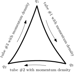
Figure 9: The schematic sketch of the Proca proton and tubes with the momentum densities whose directions are shown by the arrows.

The schematic sketch of the ‘quarks’, tubes, and directions of momenta is shown in Fig. 9. It is evident that in this case there is an angular momentum caused by the presence of the flux of the non-Abelian Proca field. Let us estimate this angular momentum as follows. Each tube has a momentum $\Pi=\mathcal{P}^{z}l_{\text{tb}}$, where $\mathcal{P}^{z}$ is the linear momentum density directed along the tube of the length $l_{\text{tb}}$, and it is calculated either using the formula (25) for the tube with classical energy flux/momentum density and a quantum flux of the longitudinal electric field or using the formula (33) for the tube with a classical flux of the longitudinal electric field and quantum energy flux/momentum density.

Let us consider the first case. Then the total angular momentum of the non-Abelian Proca field contained in the tubes can be estimated as

$$L_{g}=3\Pi r_{0}=3\mathcal{P}^{z}l_{\text{tb}}r_{0}=6\pi\frac{l_{\text{tb}}r_{0}\phi^{2}(0)}{c{g^{\prime}}^{2}}\int\limits_{0}^{\infty}x\left(\tilde{f}^{\prime}\tilde{v}^{\prime}+\frac{1}{4}\tilde{f}\tilde{v}\tilde{w}^{2}\right)dx=6\pi\frac{l_{\text{tb}}r_{0}\phi^{2}(0)}{c{g^{\prime}}^{2}}\tilde{\Pi}=12\pi\frac{\tilde{l}_{\text{tb}}\tilde{r}_{0}}{{g^{\prime}}^{2}}\frac{\hbar}{2}\tilde{\Pi},$$

where $r_{0}$ is an estimated value of the distance from the tube to the center of the Proca proton and $\tilde{l}_{\text{tb}}=l_{\text{tb}}\phi(0)/\sqrt{\hbar c},\tilde{r}_{0}=r_{0}\phi(0)/\sqrt{\hbar c}$, and ${g^{\prime}}^{2}=\hbar cg^{2}$ are dimensionless quantities.

Thus the fraction of the $\hbar/2$ Proca proton spin created by the non-Abelian Proca field contained in the tubes carrying the momentum is

$$\frac{L_{g}}{\hbar/2}=12\pi\frac{\tilde{l}_{\text{tb}}\tilde{r}_{0}}{{g^{\prime}}^{2}}\tilde{\Pi}\approx 7.2\,\pi\frac{\tilde{l}_{\text{tb}}\tilde{r}_{0}}{{g^{\prime}}^{2}}.$$

Here, we have employed the value $\tilde{\Pi}\approx 0.6$ which has been computed using the solution obtained in Sec. III.2 and shown in Fig. 8.

One can estimate the magnitude of $L_{g}/\left(\hbar/2\right)$ using natural assumptions about the values of the quantities $\tilde{l}_{\text{tb}}$ and $\tilde{r}_{0}$. Suppose that, in analogy with quantum chromodynamics, the non-Abelian-Proca-Higgs theory contains the dimensional parameter $\Lambda_{\text{nAPH}}\approx 1~{}\text{fm}^{-1}$. It is therefore natural to assume that $\phi(0)\approx\sqrt{\hbar c}\,\Lambda_{\text{nAPH}}$. The length of the tube and the distance from the tube to the center can be estimated as $l_{\text{tb}}\approx r_{0}\approx\Lambda_{\text{nAPH}}^{-1}$. As in quantum chromodynamics, let us also introduce the dimensionless coupling constant $g^{\prime}>1$; then, if one takes, say, $g^{\prime}=8.65$, the fraction of the angular momentum created by the Proca gluon field in the Proca proton spin is

$$\frac{L_{g}}{\hbar/2}\approx 30\%.$$

Thus in this section we have shown that the Proca theory permits one to explain how the Proca gluon field contributes to the Proca proton spin.

VI Summary

In the present work we have shown that there exist different types of tubes within non-Abelian Proca theory: (a) the tubes with the flux of the color electric field between ‘quarks’ located at $\pm\infty$; (b) the tubes with nonzero momentum density directed along the tube; (c) the tubes with the classical flux of the electric field and the quantum momentum density; (d) the tubes with the classical momentum density and the quantum flux of the electric field.

We have considered an imaginary particle – Proca proton – in which ‘quarks’ are connected by the tubes obtained here. Using the fact that such tubes may possess a momentum density, we have shown that in this case the angular momentum created by the tubes contributes to the Proca proton spin.

The results can be summarized as follows:

• We have obtained cylindrically symmetric solutions describing classical tubes possessing either the flux of the longitudinal electric field or the energy flux and the momentum density.

• At the qualitative level, we have shown that there can exist tubes filled simultaneously both with the flux of the longitudinal electric field and with the energy flux and the momentum density. But in this case either the flux of the longitudinal electric field or the energy flux/momentum density must be of a purely quantum nature.

• We have estimated the contribution of the Proca gluon field, contained in the tubes and creating there the momentum density, to the Proca proton spin.

References

• (1) L. Heisenberg, R. Kase, M. Minamitsuji, and S. Tsujikawa, “Hairy black-hole solutions in generalized Proca theories,” Phys. Rev. D 96, no. 8, 084049 (2017).
• (2) R. Brito, V. Cardoso, C. A. R. Herdeiro, and E. Radu, “Proca stars: Gravitating Bose-Einstein condensates of massive spin 1 particles,” Phys. Lett. B 752, 291 (2016).
• (3) C. A. R. Herdeiro, A. M. Pombo, and E. Radu, “Asymptotically flat scalar, Dirac and Proca stars: discrete vs. continuous families of solutions,” Phys. Lett. B 773, 654 (2017).
• (4) V. Dzhunushaliev and V. Folomeev, “Dirac star in the presence of Maxwell and Proca fields,” Phys. Rev. D 99, no. 10, 104066 (2019).
• (5) C. Herdeiro, I. Perapechka, E. Radu, and Y. Shnir, “Asymptotically flat spinning scalar, Dirac and Proca stars,” Phys. Lett. B 797, 134845 (2019).
• (6) L. Heisenberg, “Generalization of the Proca Action,” JCAP 1405 (2014) 015.
• (7) E. Allys, P. Peter, and Y. Rodriguez, “Generalized Proca action for an Abelian vector field,” JCAP 1602 (2016) no.02, 004.
• (8) L. Heisenberg, R. Kase, and S. Tsujikawa, “Beyond generalized Proca theories,” Phys. Lett. B 760, 617 (2016).
• (9) E. Babichev, C. Charmousis, and M. Hassaine, “Black holes and solitons in an extended Proca theory,” JHEP 1705, 114 (2017).
• (10) I. Lawrie, A Unified Grand Tour of Theoretical Physics (Institute of Physics Publishing, Bristol, 2002).
• (11) L. C. Tu, J. Luo, and G. T. Gillies, “The mass of the photon,” Rep. Prog. Phys.  68, 77 (2005).
• (12) M. Pospelov and A. Ritz, “Astrophysical Signatures of Secluded Dark Matter,” Phys. Lett. B 671, 391 (2009).
• (13) Y. Brihaye and Y. Verbin, “Proca Q Tubes and their Coupling to Gravity,” Phys. Rev. D 95, no. 4, 044027 (2017).
• (14) V. Dzhunushaliev, V. Folomeev, and A. Makhmudov, “Non-Abelian Proca-Dirac-Higgs theory: Particlelike solutions and their energy spectrum,” Phys. Rev. D 99, no. 7, 076009 (2019).
• (15) D. Singleton, “Axially symmetric solutions for SU(2) Yang-Mills theory,” J. Math. Phys. 37 (1996), 4574-4583.
• (16) Y. N. Obukhov, “Analog of black string in the Yang-Mills gauge theory,” Int. J. Theor. Phys.  37, 1455 (1998).