Majorana-mediated spin transport without spin polarization in Kitaev quantum spin liquids
Abstract
We study the spin transport through the quantum spin liquid (QSL) by investigating the real-time and real-space dynamics of the Kitaev spin system with a zigzag structure in terms of the time-dependent Majorana mean-field theory. After the magnetic field pulse is introduced to one of the edges, the spin moments are excited in the opposite edge region although no spin moments are induced in the Kitaev QSL region. This unusual spin transport originates from the fact that the spins are fractionalized into the itinerant and localized Majorana fermions in the Kitaev system. Although both Majorana fermions are excited by the magnetic pulse, only the itinerant Majorana fermions flow through the bulk regime without the spin excitation, resulting in the spin transport in the Kitaev system. We also demonstrate that this phenomenon can be observed even in the system with the Heisenberg interactions using the exact diagonalization.
Spin transport without an electric current has attracted not only practical interest in spintronics but also considerable attention in modern condensed matter physics. In insulating magnets, the carriers of the spin current are conventionally considered to be magnons, which are elementary excitations in a magnetically ordered state Uchida et al. (2010a, b); Xiao et al. (2010); Rezende et al. (2014). By contrast, the possibility of the spin transport in the quantum spin liquid (QSL) has been discussed recently. One of the typical examples is an antiferromagnetic Heisenberg spin-1/2 chain, where elementary excitations are described by the spinon with an spin. The spin Seebeck experiments for the cuprate have clarified that the spin current arises even in the QSL Hirobe et al. (2017). Therefore, the spinons, instead of the magnons, can be responsible for the spin transport in the nonmagnetic system.
Another interesting playground of the QSL is the Kitaev model Kitaev (2006), which has been studied intensively in this decade Dusuel et al. (2008); Jackeli and Khaliullin (2009); Chaloupka et al. (2010); Dhochak et al. (2010); Pedrocchi et al. (2011); Chaloupka et al. (2013); Yamaji et al. (2014); Nasu et al. (2015); Nussinov and van den Brink (2015); Suzuki et al. (2015); Schmitt and Kehrein (2015); Rousochatzakis et al. (2015); Yamaji et al. (2016); Janssen et al. (2016); Song et al. (2016); Yadav et al. (2016); Trebst (shed); Winter et al. (2017); Gohlke et al. (2017); Nasu et al. (2017); Hermanns et al. (2018); Tomishige et al. (2018); Koga et al. (2018a); Nasu et al. (2018); Knolle and Moessner (2019); Takagi et al. (2019); Lee et al. (2019); Motome and Nasu (shed). The Kitaev model consists of bond-dependent Ising interactions between spin-1/2 moments on a honeycomb lattice, and its ground state is exactly shown to be a QSL. One of the interesting features is the spin fractionalization. Namely, the spins are fractionalized into itinerant and localized Majorana fermions. Since both quasiparticles are charge neutral, the thermal transport is one of the most promising phenomena to grasp the presence of the Majorana fermions. Particularly, a half quantized plateau in the thermal quantum Hall effects has been successfully observed in the Kitaev candidate material -RuCl3 Plumb et al. (2014); Kubota et al. (2015); Sears et al. (2015); Majumder et al. (2015), which is a direct evidence of a topologically protected chiral Majorana edge mode Kasahara et al. (2018). On the other hand, less is known about the Majorana-mediated spin transport in the Kitaev QSL although it has recently been discussed in the related systems Yao and Lee (2011); de Carvalho et al. (2018); Aftergood and Takei (2019).
In the Kitaev model, spin correlations are extremely short-ranged due to the existence of the local symmetry, in contrast to the Heisenberg chain with power-low spin correlations. However, it does not necessarily mean the absence of the spin transport in the Kitaev model. When small local perturbations are present in the system, eg. the magnetic field, edges, defects, etc. the symmetry is lost in certain regions Mizoguchi and Koma (2019). Therefore, intriguing phenomena are expected to be induced in these regions. For example, the spin excitation could flow through the Kitaev QSL region without spin polarization. Thus, it is highly desired to examine the spin transport in the nonequilibrium dynamics, which should be important to observe the itinerant nature of the Majorana fermions in the bulk.
In this Letter, to address the spin transport through the Kitaev QSL, we investigate the real-time dynamics triggered by an impulse magnetic field on one of the edges. Using the time-dependent mean-field (MF) theory, we examine the time evolution of the magnetization and dynamics of the fractionalized Majorana quasiparticles. We demonstrate that a spin-polarized wavepacket created at the edge propagates to the other edge even when the two edges are separated by the QSL region without spin polarization. We also address how robust this anomalous phenomenon is against the Heisenberg interactions by means of the exact diagonalization (ED). Finally, we propose the ways to extract the results intrinsic to the Kitaev QSL with the fractionalized quasiparticles in experiments.
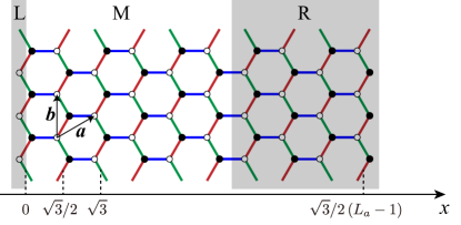
We consider the Kitaev model in the cluster of the honeycomb lattice with zigzag edges, which is schematically shown in Fig. 1. The norms of the primitive translational vectors and are assumed to be unity. The periodic boundary condition is imposed along the -direction. The system we consider here is composed of three regions. In the middle (M) region, no magnetic field is applied and the Kitaev QSL is realized without spin polarization. In the right (R) region, the static magnetic field is applied. We introduce , which is defined as the number of bonds included in this region with respect to the direction (see Fig. 1). Moreover, we term the L region composed of the left-edge sites. In this region, we introduce the time-dependent magnetic field . The corresponding Hamiltonian is
| (1) |
where is the component of an spin operator at the th site. The ferromagnetic exchange is defined on three different types of the nearest-neighbor bonds, (red), (blue), and (green) bonds (see Fig. 1).
It is known that, in the uniform lattice, the magnetic field induces the phase transition to the spin-polarized state around Nasu et al. (2018) within the MF theory. Therefore, we restrict ourselves to the case with to discuss the spin transport inherent in the Kitaev QSL.
We study the time evolution of the system upon stimuli of the magnetic pulse in the L region (see Fig. 1) Misawa et al. (2019); Misawa and Nomura (shed). To this end, we introduce the time-dependent Majorana MF theory. The details of the formulations are shown in Ref. Nasu and Motome (2019). The Hamiltonian Eq. (1) is obtained as a fermion model by applying the Jordan-Wigner transformation to the spin operators Chen and Hu (2007); Feng et al. (2007); Chen and Nussinov (2008). Furthermore, by introducing two kinds of Majorana fermions, and , from a complex fermion at each site, Eq. (1) is rewritten as
| (2) | |||||
where indicates the position of the bond (the center of the bond; see Fig. 1). and ( and ) are the Majorana fermion operators connected with the bond in the sublattice (), as shown in Fig. 1. When , at each , and is the local conserved quantity. In the case, the model is solvable as the Hamiltonian is bilinear in terms of , and its low-energy dispersion is given as around the K point with the velocity . This indicates that and are regarded as the itinerant and localized Majorana fermions, respectively.
Since the magnetic field hybridizes two kinds of the Majorana fermions, the Hamiltonian is no longer exactly solvable. Here, we apply the Hartree-Fock type decoupling to the interaction on the bond as , where we have introduced the six kinds of - and -dependent MFs as , , , , , , where is the horizontal coordinate of and . This MF theory is exact when . Therefore, we believe that our MF results are reliable as far as the small fields are applied. In the MF theory, the many-body wave function is expressed as a direct product of one-body states, whose time-evolution is described by the MF Hamiltonian. Determining the MFs at each time from the many-body wave function, we compute the time-evolution of the one-body states with the extended Euler method Terai and Ono (1993); Hirano and Ono (2000); Tanaka and Yonemitsu (2010); Ohara and Yamamoto (2017); Tanaka et al. (2018); Seo et al. (2018). The time-dependent magnetic field is explicitly given as, , where and are constants for the Gaussian pulse. In the following, we fix the system size as and , the static field as , and pulse parameters as and .
Before discussing the spin transport through the M region, we examine the system without this region, namely, the static magnetic field is applied to the sites in the R region with . In this case, there are no local conserved quantities, leading to nonzero local spin moments. Figure 2(a) shows the contour plot of the changes in the spin moments , where . As expected, we find that the wavepacket created by the magnetic-field pulse flows to the right edge. Note that its velocity almost coincides with the Majorana velocity of the genuine Kitaev model, , which is shown as the dashed line in Fig. 2(a). This indicates that the propagation is attributed to the gapless Majorana excitation in the bulk within a small static field.
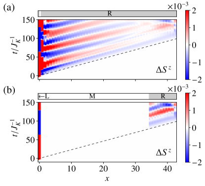
Now, we consider the real-time dynamics of the nonmagnetic Kitaev spin system triggered by the magnetic-field pulse at the left edge to discuss how the wavepacket flows through the M region (the Kitaev QSL without spin polarization). In this region, the local conserved quantity is present in each hexagon, and spin correlations are extremely short-ranged Baskaran et al. (2007). Figure 2(b) shows the time evolution of in the system with . We find that the magnetic moment is always zero in the M region and no proximity effect is found around the interface between L and M regions. Nevertheless, in the R region, is induced and the wavepacket flows with the Majorana velocity . This result indicates that the spin excitations propagate in the nonmagnetic region via the itinerant Majorana fermions, which cannot be explained by classical pictures such as the spin wave theory.
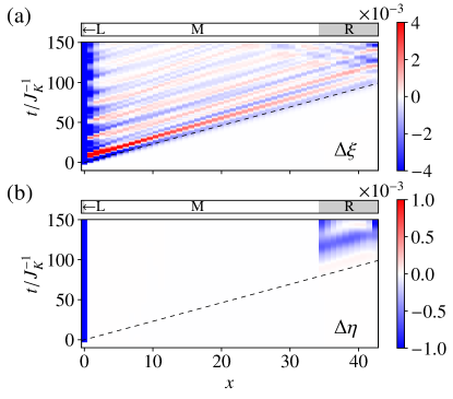
To discuss the propagation of the spin excitation through the QSL region in more detail, we examine the time evolutions of and , which correspond to the dynamics of itinerant and localized Majorana fermions, as shown in Figs. 3(a) and 3(b). We find in Fig. 3(a) that the excitation created in the left edge at propagates in the whole region, which results from the motion of the itinerant Majorana fermions. By contrast, Fig. 3(b) shows that vanishes in the M region owing to the existence of the local symmetry, while it appears in the R region. This is the similar behavior as in . These suggest that, after the excitation at the left edge, only the itinerant Majorana fermions propagate in the bulk, where no oscillation appears in the magnetization, and finally reach the R region. The weak magnetic field in the R region yields the hybridization between the itinerant Majorana fermions and the localized fermions, resulting in time-dependent nonzero spin moments there. Thus, in the Kitaev QSL, the spin transport is mediated by the Majorana fermions although the spin moments never appear. Moreover, we have confirmed that the magnitude of the spin moment induced in the R region exhibits a power-low decay as a function of the length of the M region. This is ascribed to the gapless dispersion of the Majorana fermions, in contrast to the existence of the gap in the spin excitation in the Kitaev model.
The pulse-amplitude dependence in this phenomenon is also remarkable. In the R region, turns out to be proportional to . This can be explained by considering the local symmetry at the left edge pro . This non-linear feature is intrinsic in the Kitaev model, in contrast to the conventional systems with . To study how visible anomalous behavior is in the system with the Heisenberg interaction, we apply the ED method to the Hamiltonian with the antiferromagnetic Heisenberg coupling . It is known that, when , the Kitaev QSL is stable against small Chaloupka et al. (2010, 2013); Yamaji et al. (2016); Gohlke et al. (2017). In our calculations, the initial ground state is obtained with the Lanczos method and the time evolution is simply evaluated by the Runge-Kutta method.
The obtained results for the 24-site cluster with , , and are shown in Fig. 3. In the calculations, we have confirmed that the induced moment is always parallel to the direction.
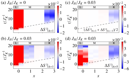
First, we show the results for the genuine Kitaev model with in Fig. 4(a). One can find the propagation of the magnetic excitation from one edge to the other through the QSL region without spin polarization, which is consistent with the Majorana MF result discussed above. In the presence of the Heisenberg term (), takes nonzero values in the M region, as shown in Fig. 4(b), suggesting that the Heisenberg interaction affects the flow of the spin excitation. In particular, the spin modulation in the M region is more prominent compared to that in the R region. This difference from the genuine Kitaev model originates from the fact that the Heisenberg interaction yields the interaction between itinerant and localized Majorana fermions. Therefore, the spin moments appear in the M region near the interface to the L region as a proximity effect, as shown in Fig. 4(b).
We note that in the R region is similar to the case without the Heisenberg interactions. This implies that the spin transport inherent in the Kitaev model still survives. It is naively expected that in the M and R region, the Heisenberg and Kitaev interactions mainly give and contributions in the spin oscillation, as discussed above. Therefore, the unique feature for the Kitaev system is extracted by examining the average of the magnetic responses after the magnetic pulses with and . In Fig. 4(c), this quantity is hardly seen in the M region but clearly observed in the R region, which is a consequence of the Kitaev QSL with itinerant Majorana fermions.
When the pulse amplitude is relatively large, the Kitaev interaction plays a dominant role for the spin propagation and the spin transport without spin polarization becomes practically prominent. Figure 4(d) presents the results with the large . The spin moments induced in the M region are relatively small, but the spin excitation propagates to the right edge, at which the spin moments induced are much larger than those in the M region. This phenomenon is essentially the same as that in the genuine Kitaev case shown in Fig. 4(a). The above two results suggest that the spin transport mediated by the fractionalized itinerant quasiparticles without spin excitations can be observed even in the presence of additional interactions.
Finally, we discuss the relevance of the present results to real materials. The setup of our study could be implemented by considering a Kitaev candidate material sandwiched by ferromagnetic insulators. The candidate materials have been proposed as IrO3 (A=Na, Li) Singh and Gegenwart (2010); Singh et al. (2012); Comin et al. (2012); Choi et al. (2012); Takayama et al. (2015); Kitagawa et al. (2018) and -RuCl3 Plumb et al. (2014); Kubota et al. (2015); Sears et al. (2015); Majumder et al. (2015). The stimuli of the magnetic field pulse can be injected from a ferromagnetic insulator by the spin pumping Kajiwara et al. (2010); Sandweg et al. (2011); Heinrich et al. (2011); Hahn et al. (2013) or circular polarized light irradiation Kimel et al. (2005); Stanciu et al. (2007). Our results suggest that the spin-excited flow propagates to the other edge even if the magnetic polarization is absent in the Kitaev magnet, and therefore, we expect that the time-dependent magnetic moment is observed in the ferromagnetic insulator connected to the other side of the Kitaev magnet with a small overlapping. This time evolution can be experimentally measured by the Kerr or Faraday rotations Hiebert et al. (1997); Kimel et al. (2005), which will provide convincing evidence of the fractionalized itinerant quasiparticles in the bulk of the Kitaev magnet.
Note that in the real system, a magnetic order hinders the appearance of the Kitaev QSL Liu et al. (2011); Ye et al. (2012); Johnson et al. (2015); Cao et al. (2016); Freund et al. (2016); Williams et al. (2016). This effect can be avoided by the finite temperature measurement above the Néel temperature, where the itinerant quasiparticles are active, and/or the recent progress of the thin film Yamaji et al. (2014); Winter et al. (2016); Weber et al. (2016); Ziatdinov et al. (2016); Grönke et al. (2018); Zhou et al. (2019a, b); Mashhadi et al. (2019); Gerber et al. (shed); Biswas et al. (shed), which suppresses the magnetic ordering due to the suppression of the interlayer coupling. Moreover, by changing the intensity of the injection of the spin excitation, one could estimate the magnitude of the additional interactions such the Heisenberg one. The effect of the off-diagonal interactions, so called term, is not addressed in the present study but we expect that this gives a similar effect to the Heisenberg one Rau et al. (2014); Rusnačko et al. (2019); Gordon et al. (2019).
In summary, we have demonstrated that, after the magnetic excitation at one of the edges in the Kitaev spin system, the spin moments never appear in the bulk, but are fluctuated in the opposite edge. We have revealed that this unusual spin transport is governed by the fractionalized itinerant Majorana fermions. The spin transport without spin polarization should be visible even in the system with the Heisenberg coupling by using the pulse field dependence in .
We also note that it might be possible to control the motion of the localized Majorana fermions (vison) in the bulk, by switching on/off the magnetic field. This should be important for realizing the vison transport in the experiments. It is also interesting to study the spin transport in the generalized Kitaev models Baskaran et al. (2008); Koga et al. (2018b); Minakawa et al. (2019), where the existence of spin fractionalization has also been suggested Koga et al. (2018b); Oitmaa et al. (2018); Koga and Nasu (2019). The real-time spin dynamics should be one of the possible candidates to clarify the presence of the quasiparticles.
Acknowledgements.
The authors thank T. Mizoguchi and M. Udagawa for fruitful discussions. Parts of the numerical calculations were performed in the supercomputing systems in ISSP, the University of Tokyo. This work was supported by Grant-in-Aid for Scientific Research from JSPS, KAKENHI Grant Nos. JP19K23425 (Y.M.), JP19H05821, JP18K04678, JP17K05536 (A.K.), JP16H02206, JP18H04223, JP19K03742 (J.N.), by JST CREST Grant No. JPMJCR1901 (Y.M.) and by JST PREST (JPMJPR19L5) (J.N.).References
- Uchida et al. (2010a) K.-i. Uchida, H. Adachi, T. Ota, H. Nakayama, S. Maekawa, and E. Saitoh, Appl. Phys. Lett. 97, 172505 (2010a).
- Uchida et al. (2010b) K.-i. Uchida, J. Xiao, H. Adachi, J.-i. Ohe, S. Takahashi, J. Ieda, T. Ota, Y. Kajiwara, H. Umezawa, H. Kawai, et al., Nat. Mater. 9, 894 (2010b).
- Xiao et al. (2010) J. Xiao, G. E. W. Bauer, K.-c. Uchida, E. Saitoh, and S. Maekawa, Phys. Rev. B 81, 214418 (2010).
- Rezende et al. (2014) S. M. Rezende, R. L. Rodríguez-Suárez, R. O. Cunha, A. R. Rodrigues, F. L. A. Machado, G. A. Fonseca Guerra, J. C. Lopez Ortiz, and A. Azevedo, Phys. Rev. B 89, 014416 (2014).
- Hirobe et al. (2017) D. Hirobe, M. Sato, T. Kawamata, Y. Shiomi, K.-i. Uchida, R. Iguchi, Y. Koike, S. Maekawa, and E. Saitoh, Nat. Phys. 13, 30 (2017).
- Kitaev (2006) A. Kitaev, Ann, Phys. 321, 2 (2006).
- Dusuel et al. (2008) S. Dusuel, K. P. Schmidt, and J. Vidal, Phys. Rev. Lett. 100, 177204 (2008).
- Jackeli and Khaliullin (2009) G. Jackeli and G. Khaliullin, Phys. Rev. Lett. 102, 017205 (2009).
- Chaloupka et al. (2010) J. Chaloupka, G. Jackeli, and G. Khaliullin, Phys. Rev. Lett. 105, 027204 (2010).
- Dhochak et al. (2010) K. Dhochak, R. Shankar, and V. Tripathi, Phys. Rev. Lett. 105, 117201 (2010).
- Pedrocchi et al. (2011) F. L. Pedrocchi, S. Chesi, and D. Loss, Phys. Rev. B 84, 165414 (2011).
- Chaloupka et al. (2013) J. Chaloupka, G. Jackeli, and G. Khaliullin, Phys. Rev. Lett. 110, 097204 (2013).
- Yamaji et al. (2014) Y. Yamaji, Y. Nomura, M. Kurita, R. Arita, and M. Imada, Phys. Rev. Lett. 113, 107201 (2014).
- Nasu et al. (2015) J. Nasu, M. Udagawa, and Y. Motome, Phys. Rev. B 92, 115122 (2015).
- Nussinov and van den Brink (2015) Z. Nussinov and J. van den Brink, Rev. Mod. Phys. 87, 1 (2015).
- Suzuki et al. (2015) T. Suzuki, T. Yamada, Y. Yamaji, and S.-i. Suga, Phys. Rev. B 92, 184411 (2015).
- Schmitt and Kehrein (2015) M. Schmitt and S. Kehrein, Phys. Rev. B 92, 075114 (2015).
- Rousochatzakis et al. (2015) I. Rousochatzakis, J. Reuther, R. Thomale, S. Rachel, and N. B. Perkins, Phys. Rev. X 5, 041035 (2015).
- Yamaji et al. (2016) Y. Yamaji, T. Suzuki, T. Yamada, S.-i. Suga, N. Kawashima, and M. Imada, Phys. Rev. B 93, 174425 (2016).
- Janssen et al. (2016) L. Janssen, E. C. Andrade, and M. Vojta, Phys. Rev. Lett. 117, 277202 (2016).
- Song et al. (2016) X.-Y. Song, Y.-Z. You, and L. Balents, Phys. Rev. Lett. 117, 037209 (2016).
- Yadav et al. (2016) R. Yadav, N. A. Bogdanov, V. M. Katukuri, S. Nishimoto, J. Van Den Brink, and L. Hozoi, Sci. Rep. 6, 37925 (2016).
- Trebst (shed) S. Trebst, preprint , arXiv:1701.07056 (unpublished).
- Winter et al. (2017) S. M. Winter, A. A. Tsirlin, M. Daghofer, J. van den Brink, Y. Singh, P. Gegenwart, and R. Valentí, J. Phys. Condens. Matter 29, 493002 (2017).
- Gohlke et al. (2017) M. Gohlke, R. Verresen, R. Moessner, and F. Pollmann, Phys. Rev. Lett. 119, 157203 (2017).
- Nasu et al. (2017) J. Nasu, J. Yoshitake, and Y. Motome, Phys. Rev. Lett. 119, 127204 (2017).
- Hermanns et al. (2018) M. Hermanns, I. Kimchi, and J. Knolle, Ann. Rev. Condens. Matter Phys. 9, 17 (2018).
- Tomishige et al. (2018) H. Tomishige, J. Nasu, and A. Koga, Phys. Rev. B 97, 094403 (2018).
- Koga et al. (2018a) A. Koga, S. Nakauchi, and J. Nasu, Phys. Rev. B 97, 094427 (2018a).
- Nasu et al. (2018) J. Nasu, Y. Kato, Y. Kamiya, and Y. Motome, Phys. Rev. B 98, 060416(R) (2018).
- Knolle and Moessner (2019) J. Knolle and R. Moessner, Ann. Rev. Condens. Matter Phys. 10, 451 (2019).
- Takagi et al. (2019) H. Takagi, T. Takayama, G. Jackelli, G. Khaliullin, and S. Nagler, Nat. Rev. Phys. 1, 264 (2019).
- Lee et al. (2019) H.-Y. Lee, R. Kaneko, T. Okubo, and N. Kawashima, Phys. Rev. Lett. 123, 087203 (2019).
- Motome and Nasu (shed) Y. Motome and J. Nasu, preprint , arXiv:1909.02234 (unpublished).
- Plumb et al. (2014) K. W. Plumb, J. P. Clancy, L. J. Sandilands, V. V. Shankar, Y. F. Hu, K. S. Burch, H.-Y. Kee, and Y.-J. Kim, Phys. Rev. B 90, 041112(R) (2014).
- Kubota et al. (2015) Y. Kubota, H. Tanaka, T. Ono, Y. Narumi, and K. Kindo, Phys. Rev. B 91, 094422 (2015).
- Sears et al. (2015) J. A. Sears, M. Songvilay, K. W. Plumb, J. P. Clancy, Y. Qiu, Y. Zhao, D. Parshall, and Y.-J. Kim, Phys. Rev. B 91, 144420 (2015).
- Majumder et al. (2015) M. Majumder, M. Schmidt, H. Rosner, A. A. Tsirlin, H. Yasuoka, and M. Baenitz, Phys. Rev. B 91, 180401(R) (2015).
- Kasahara et al. (2018) Y. Kasahara, T. Ohnishi, Y. Mizukami, O. Tanaka, S. Ma, K. Sugii, N. Kurita, H. Tanaka, J. Nasu, Y. Motome, T. Shibauchi, and Y. Matsuda, Nature 559, 227 (2018).
- Yao and Lee (2011) H. Yao and D.-H. Lee, Phys. Rev. Lett. 107, 087205 (2011).
- de Carvalho et al. (2018) V. S. de Carvalho, H. Freire, E. Miranda, and R. G. Pereira, Phys. Rev. B 98, 155105 (2018).
- Aftergood and Takei (2019) J. Aftergood and S. Takei, preprint , arXiv:1910.08610 (2019).
- Mizoguchi and Koma (2019) T. Mizoguchi and T. Koma, Phys. Rev. B 99, 184418 (2019).
- Misawa et al. (2019) T. Misawa, R. Nakai, and K. Nomura, Phys. Rev. B 100, 155123 (2019).
- Misawa and Nomura (shed) T. Misawa and K. Nomura, preprint , arXiv:1907.10459 (unpublished).
- Nasu and Motome (2019) J. Nasu and Y. Motome, Phys. Rev. Research 1, 033007 (2019).
- Chen and Hu (2007) H.-D. Chen and J. Hu, Phys. Rev. B 76, 193101 (2007).
- Feng et al. (2007) X.-Y. Feng, G.-M. Zhang, and T. Xiang, Phys. Rev. Lett. 98, 087204 (2007).
- Chen and Nussinov (2008) H.-D. Chen and Z. Nussinov, J. Phys. A 41, 075001 (2008).
- Terai and Ono (1993) A. Terai and Y. Ono, Progress of Theoretical Physics Supplement 113, 177 (1993).
- Hirano and Ono (2000) Y. Hirano and Y. Ono, J. Phys. Soc. Jpn. 69, 2131 (2000).
- Tanaka and Yonemitsu (2010) Y. Tanaka and K. Yonemitsu, J. Phys. Soc. Jpn. 79, 024712 (2010).
- Ohara and Yamamoto (2017) J. Ohara and S. Yamamoto, J. Phys.: Conf. Ser. 868, 012013 (2017).
- Tanaka et al. (2018) Y. Tanaka, M. Daira, and K. Yonemitsu, Phys. Rev. B 97, 115105 (2018).
- Seo et al. (2018) H. Seo, Y. Tanaka, and S. Ishihara, Phys. Rev. B 98, 235150 (2018).
- Baskaran et al. (2007) G. Baskaran, S. Mandal, and R. Shankar, Phys. Rev. Lett. 98, 247201 (2007).
- (57) This can be explained as follows. Since the system has the local symmetry before and after the introduction of the pulsed field, each eigenstate is specified by a set of the eigenvalues of in the L region. Let us start with the initial state given as . After the pulse at the left-edge, the final state should be given within the first-order perturbation as , where is some constant and and belong to the distinct subspaces specified by different sets of eigenvalues of at the left edge. On the other hand, when some operator commutes with at the left edge, belongs to the same subspace as . (For example, is ,or in the M and R regimes.) Therefore, the first order component of in vanishes.
- Singh and Gegenwart (2010) Y. Singh and P. Gegenwart, Phys. Rev. B 82, 064412 (2010).
- Singh et al. (2012) Y. Singh, S. Manni, J. Reuther, T. Berlijn, R. Thomale, W. Ku, S. Trebst, and P. Gegenwart, Phys. Rev. Lett. 108, 127203 (2012).
- Comin et al. (2012) R. Comin, G. Levy, B. Ludbrook, Z.-H. Zhu, C. N. Veenstra, J. A. Rosen, Y. Singh, P. Gegenwart, D. Stricker, J. N. Hancock, D. van der Marel, I. S. Elfimov, and A. Damascelli, Phys. Rev. Lett. 109, 266406 (2012).
- Choi et al. (2012) S. K. Choi, R. Coldea, A. N. Kolmogorov, T. Lancaster, I. I. Mazin, S. J. Blundell, P. G. Radaelli, Y. Singh, P. Gegenwart, K. R. Choi, S.-W. Cheong, P. J. Baker, C. Stock, and J. Taylor, Phys. Rev. Lett. 108, 127204 (2012).
- Takayama et al. (2015) T. Takayama, A. Kato, R. Dinnebier, J. Nuss, H. Kono, L. S. I. Veiga, G. Fabbris, D. Haskel, and H. Takagi, Phys. Rev. Lett. 114, 077202 (2015).
- Kitagawa et al. (2018) K. Kitagawa, T. Takayama, Y. Matsumoto, A. Kato, R. Takano, Y. Kishimoto, S. Bette, R. Dinnebier, G. Jackeli, and H. Takagi, Nature 554, 341 (2018).
- Kajiwara et al. (2010) Y. Kajiwara, K. Harii, S. Takahashi, J.-i. Ohe, K. Uchida, M. Mizuguchi, H. Umezawa, H. Kawai, K. Ando, K. Takanashi, et al., Nature 464, 262 (2010).
- Sandweg et al. (2011) C. W. Sandweg, Y. Kajiwara, A. V. Chumak, A. A. Serga, V. I. Vasyuchka, M. B. Jungfleisch, E. Saitoh, and B. Hillebrands, Phys. Rev. Lett. 106, 216601 (2011).
- Heinrich et al. (2011) B. Heinrich, C. Burrowes, E. Montoya, B. Kardasz, E. Girt, Y.-Y. Song, Y. Sun, and M. Wu, Phys. Rev. Lett. 107, 066604 (2011).
- Hahn et al. (2013) C. Hahn, G. de Loubens, O. Klein, M. Viret, V. V. Naletov, and J. Ben Youssef, Phys. Rev. B 87, 174417 (2013).
- Kimel et al. (2005) A. Kimel, A. Kirilyuk, P. Usachev, R. Pisarev, A. Balbashov, and T. Rasing, Nature 435, 655 (2005).
- Stanciu et al. (2007) C. D. Stanciu, F. Hansteen, A. V. Kimel, A. Kirilyuk, A. Tsukamoto, A. Itoh, and T. Rasing, Phys. Rev. Lett. 99, 047601 (2007).
- Hiebert et al. (1997) W. K. Hiebert, A. Stankiewicz, and M. R. Freeman, Phys. Rev. Lett. 79, 1134 (1997).
- Liu et al. (2011) X. Liu, T. Berlijn, W.-G. Yin, W. Ku, A. Tsvelik, Y.-J. Kim, H. Gretarsson, Y. Singh, P. Gegenwart, and J. P. Hill, Phys. Rev. B 83, 220403(R) (2011).
- Ye et al. (2012) F. Ye, S. Chi, H. Cao, B. C. Chakoumakos, J. A. Fernandez-Baca, R. Custelcean, T. F. Qi, O. B. Korneta, and G. Cao, Phys. Rev. B 85, 180403(R) (2012).
- Johnson et al. (2015) R. D. Johnson, S. C. Williams, A. A. Haghighirad, J. Singleton, V. Zapf, P. Manuel, I. I. Mazin, Y. Li, H. O. Jeschke, R. Valentí, and R. Coldea, Phys. Rev. B 92, 235119 (2015).
- Cao et al. (2016) H. B. Cao, A. Banerjee, J.-Q. Yan, C. A. Bridges, M. D. Lumsden, D. G. Mandrus, D. A. Tennant, B. C. Chakoumakos, and S. E. Nagler, Phys. Rev. B 93, 134423 (2016).
- Freund et al. (2016) F. Freund, S. Williams, R. Johnson, R. Coldea, P. Gegenwart, and A. Jesche, Sci. Rep. 6, 35362 (2016).
- Williams et al. (2016) S. C. Williams, R. D. Johnson, F. Freund, S. Choi, A. Jesche, I. Kimchi, S. Manni, A. Bombardi, P. Manuel, P. Gegenwart, and R. Coldea, Phys. Rev. B 93, 195158 (2016).
- Winter et al. (2016) S. M. Winter, Y. Li, H. O. Jeschke, and R. Valentí, Phys. Rev. B 93, 214431 (2016).
- Weber et al. (2016) D. Weber, L. M. Schoop, V. Duppel, J. M. Lippmann, J. Nuss, and B. V. Lotsch, Nano Letters 16, 3578 (2016).
- Ziatdinov et al. (2016) M. Ziatdinov, A. Banerjee, A. Maksov, T. Berlijn, W. Zhou, H. Cao, J.-Q. Yan, C. A. Bridges, D. Mandrus, S. E. Nagler, et al., Nat. Commun. 7, 13774 (2016).
- Grönke et al. (2018) M. Grönke, P. Schmidt, M. Valldor, S. Oswald, D. Wolf, A. Lubk, B. Büchner, and S. Hampel, Nanoscale 10, 19014 (2018).
- Zhou et al. (2019a) B. Zhou, Y. Wang, G. B. Osterhoudt, P. Lampen-Kelley, D. Mandrus, R. He, K. S. Burch, and E. A. Henriksen, J. Phys. Chem. Solids 128, 291 (2019a).
- Zhou et al. (2019b) B. Zhou, J. Balgley, P. Lampen-Kelley, J.-Q. Yan, D. G. Mandrus, and E. A. Henriksen, Phys. Rev. B 100, 165426 (2019b).
- Mashhadi et al. (2019) S. Mashhadi, Y. Kim, J. Kim, D. Weber, T. Taniguchi, K. Watanabe, N. Park, B. V. Lotsch, J. H. Smet, M. Burghard, et al., Nano Letters (2019).
- Gerber et al. (shed) E. Gerber, Y. Yao, T. A. Arias, and E.-A. Kim, preprint , arXiv:1902.09550 (unpublished).
- Biswas et al. (shed) S. Biswas, Y. Li, S. M. Winter, J. Knolle, and R. Valentí, preprint , arXiv:1902.09550 (unpublished).
- Rau et al. (2014) J. G. Rau, E. K.-H. Lee, and H.-Y. Kee, Phys. Rev. Lett. 112, 077204 (2014).
- Rusnačko et al. (2019) J. Rusnačko, D. Gotfryd, and J. Chaloupka, Phys. Rev. B 99, 064425 (2019).
- Gordon et al. (2019) J. S. Gordon, A. Catuneanu, E. S. Sørensen, and H.-Y. Kee, Nat. Commun. 10, 2470 (2019).
- Baskaran et al. (2008) G. Baskaran, D. Sen, and R. Shankar, Phys. Rev. B 78, 115116 (2008).
- Koga et al. (2018b) A. Koga, H. Tomishige, and J. Nasu, J. Phys. Soc. Jpn. 87, 063703 (2018b).
- Minakawa et al. (2019) T. Minakawa, J. Nasu, and A. Koga, Phys. Rev. B 99, 104408 (2019).
- Oitmaa et al. (2018) J. Oitmaa, A. Koga, and R. R. P. Singh, Phys. Rev. B 98, 214404 (2018).
- Koga and Nasu (2019) A. Koga and J. Nasu, Phys. Rev. B 100, 100404(R) (2019).