Adaptive flow-level scheduling for the IoT MAC

Abstract

Over the past decade, distributed CSMA, which forms the basis for WiFi, has been deployed ubiquitously to provide seamless and high-speed mobile internet access. However, distributed CSMA might not be ideal for future IoT/M2M applications, where the density of connected devices/sensors/controllers is expected to be orders of magnitude higher than that in present wireless networks. In such high-density networks, the overhead associated with completely distributed MAC protocols will become a bottleneck. Moreover, IoT communications are likely to have strict QoS requirements, for which the ‘best-effort’ scheduling by present WiFi networks may be unsuitable. This calls for a clean-slate redesign of the wireless MAC taking into account the requirements for future IoT/M2M networks. In this paper, we propose a reservation-based (for minimal overhead) wireless MAC designed specifically with IoT/M2M applications in mind. The key features include: (i) flow-level, rather than packet level contention to minimize overhead, (ii) deadline aware, reservation based scheduling, and (iii) the ability to dynamically adapt the MAC parameters with changing workload.

I Introduction

Over the past decade, WiFi has become the mainstay of non-cellular wireless communication. It has been deployed widely across residential as well as enterprise settings to provide seamless and high-speed mobile internet access. It is estimated that over 94 million WiFi hotspots were deployed worldwide as of 2016.

WiFi is based on CSMA/CA (Carrier Sense Multiple Access/Collision Avoidance) — an entirely distributed medium access mechanism based on channel sensing and collision avoidance using randomized backoff [1]. The protocol operates at the link layer, providing a best-effort delivery of packets from transmitter to receiver. In line with the layered approach to networking, WiFi is oblivious to the end-to-end flows that generate the packets it delivers, and is therefore also blind to their Quality of Service (QoS) requirements. However, WiFi works remarkably well in the settings in which it is predominantly deployed: a moderate number of end-nodes requiring high data-rate connected to each access point.

However, several upcoming application scenarios differ considerably from the settings in which WiFi is presently deployed. The explosion of interest in the Internet of Things (IoT) and Machine to Machine (M2M) communication points to scenarios where the density of connected devices is projected to grow manifold in the coming years. These IoT devices, which include household appliances, healthcare devices, smart cars, sensors and actuators, will require reliable, but not necessarily very high-speed internet access. In other words, in contrast to current WiFi deployments, we should expect a considerable growth in the number of wireless end-devices, each of which will generate moderate, intermittent, but time-bound traffic. In such a setting, the overhead associated with the entirely distributed and packet-level WiFi MAC is likely to become a bottleneck. Moreover, this overhead, due to frequent collisions between end-nodes attempting to access the channel, would also be energy inefficient, which is a concern given that many IoT devices are likely to be power constrained.

This paper proposes an alternative framework for MAC design, particularly suited for upcoming IoT/M2M application settings: A large number of wireless nodes connected to the internet via a single access point, each generating moderate, occasional, but QoS sensitive traffic. The proposed framework is based on Time Slotted Channel Hopping (TSCH), which is supported under the IEEE 802.15.4e specification [2]. The key features of the proposed framework are:

1. The scheduling (specifically, admission control) is flow-aware, where a flow refers to a single burst of data generated by an IoT device.

2. Packet-level scheduling is performed centrally in an entirely reservation-based, QoS-aware manner, using ideas from the deadline scheduling literature for real-time systems.

3. Contention only takes place when the end-nodes attempt to register their flows with the access point. This reduces protocol overhead (relative to a MAC where contention takes place for the transmission of each packet). Once a flow is admitted, it is centrally scheduled by the access point such that it meets its deadline.

4. The MAC parameters are dynamically adapted to the (possibly time-varying) traffic characteristics.

5. The framework supports highly heterogeneous end-devices, with widely ranging traffic patterns and energy constraints.

As we demonstrate, the combination of flow-level, QoS-aware admission control, and centralized reservation-based packet scheduling results in a considerable gain in throughput as well as energy efficiency relative to CSMA/CA.

It should be noted that while the primary intent of this paper is to propose an alternative framework for MAC design for IoT/M2M applications, we describe an example protocol based on this framework with sufficient algorithmic and implementation detail to enable a comparison with CSMA/CA.

The remainder of this paper is organised as follows. We describe the setting for our MAC framework in Section II, the admission control and scheduling aspects of the proposed framework in Section III, and the parameter adaptation aspects in Section IV. Finally, we evaluate the performance of the proposed framework alongside CSMA/CA in Section V.

State of the art

Several papers have explored reservation-based wireless MAC designs. The paper closest to the present one is [3], which also proposes a flow-level, deadline scheduling based MAC design. However, in contrast with this work, [3] only considers a single channel. Indeed, the possibility of scheduling over multiple channels considerably complicates the deadline scheduling problem [4]. Another related work is [5], which considers the problem of real-time scheduling of periodic flows (as opposed to the ‘burst’ flows considered here) in a multi-hop, single channel setting.

The papers [6] and [7] consider the problem of decentralized slot reservation in a multi-hop environment. While [6] considers only a single channel, [7] considers the multi-channel TSCH model as in the present paper. However, both these papers consider packet-level reservation, as opposed to the flow-level reservation considered here. Moreover, neither of the above papers consider deadline-aware scheduling.

We are unaware of any work that considers the problem of deadline constrained flow-level reservation in a multi-channel setting. Moreover, none of the above papers consider online MAC parameter adaptation, which is one of the key features of the present work.

Finally, we note that several standards have been proposed for IoT/M2M applications. While a comprehensive survey of these is beyond the scope of the present paper due to space constraints, we note here that 802.11ah and 802.15.4e are among the prominent standards in this space. 802.15.4e supports TSCH, upon which the proposed framework is based.

II Setting for MAC design

In this section, we describe the setting for the proposed MAC design.

II-A Topology

We consider a single-hop (star) topology, with a large number of IoT nodes connected wirelessly to a central master node (a.k.a. hub, access point). The master node has broadband access to the internet (either wired or wireless), and is responsible for routing the traffic generated by the IoT nodes to the intended destinations over the internet. The IoT nodes may be heterogeneous in the nature of traffic generated, their QoS requirements, as well as their power constraints.

The above may capture a residential setting, where all IoT devices in a household including appliances and healthcare sensors communicate with a single access point, or an industrial setting, where all the different sensors and actuators on a factory floor communicate with a central controller.

II-B Traffic model

The IoT nodes generate flows (transmission requests) sporadically, which need to be transmitted to the master node. Each flow $i$ is characterized by a load $l_{i},$ which denotes the number of packets that comprise the flow, and a deadline $d_{i},$ which is the maximum delay that can be incurred in transmitting all the $l_{i}$ packets to the master node. A flow is considered to be successful if its load is served (i.e., all its packets are transmitted to the master) within its deadline.

The setting of interest is one where the number of IoT nodes connected to the master is large, but each node generates flows only occasionally. This is analogous to the case of telephone networks, where a single switch (in the wireline setting) or base station (in the wireless setting) serves a large number of subscribers, who generate call requests occasionally. Thus, borrowing the modelling framework from telephone networks, we assume that the generation of flows (by all the IoT nodes connected to the master) follows a Poisson process of rate $\lambda.$ We note that the assumption of Poisson arrivals is well backed by both theoretical justification as well as empirical evidence [8, Chapter 11].

II-C Frame Structure

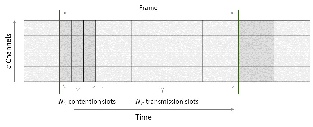
Figure 1: Structure of a frame in proposed MAC design

The proposed MAC design is based on Time Slotted Channel Hopping (TSCH). Let $c$ denote the number of channels the protocol operates on. These channels are assumed to be identical in capacity. It is further assumed that an IoT node can transmit/receive on only a single channel at a time, whereas the master node can receive on all $c$ channels simultaneously. Time is divided into frames, each frame consisting of a contention phase (for new flows to get admitted with the master) and a transmission phase (when the actual packet transmissions take place); see Figure 1.

Specifically, the contention phase consists of $N_{C}$ contention slots, each one time unit long. The transmission phase consists of $N_{T}$ transmission slots, each $k$ time units long, where $k>1$ is an integer. Each transmission slot can support a single packet transmission. Thus, the length of the frame equals $T=N_{C}+kN_{T}$ time units.

Note that there are $cN_{C}$ contention blocks in each frame (a block referring to a time slot on a particular channel); these are used by newly arrived flows to register with the master, as described in Section III. The master performs admission control, and schedules the accepted flows in the transmission phase, taking into account the deadlines of the different accepted flows (details in Section III). Note that there are $cN_{T}$ transmission blocks in each frame.

III Admission Control and Scheduling

In this section, we present the details of the proposed MAC design, including the contention process for newly generated flows, admission control, and scheduling of admitted flows. The adaptation of the MAC parameters based on the observed traffic characteristics is described in Section IV.

III-A Contention

As noted in Section II, we assume that flows are generated by the IoT nodes according to a Poisson process of rate $\lambda.$ Each generated flow $i$ is associated with the tuple $(t_{i},l_{i},d_{i}),$ where $t_{i}$ denotes the generation time, $l_{i}$ denotes the load measured in number of packets (i.e., number of transmission blocks required by the flow), and $d_{i}$ denotes the deadline (i.e., the flow must complete all $l_{i}$ transmissions until time $t_{i}+d_{i}$ in order to be considered successful).

The proposed contention mechanism works as follows. Each flow that is generated over the duration of any frame has the chance to contend for admission during the contention phase of the following frame. Specifically, each flow contends for admission with probability $p,$ where $p,$ which we refer to as the contention probability, is a protocol parameter whose value is determined (and broadcast periodically) by the master node. Each contending flow $i$ picks a contention block (out of the $cN_{C}$ possibilities) uniformly at random, and transmits an admission request in that block, which contains all relevant flow information, including the tuple $(t_{i},l_{i},d_{i}).$ If multiple contending nodes pick the same contention block, their admission requests collide and are not received by the master. On the other hand, if a certain contention block is selected by exactly one contending flow, its admission request is received by the master, and is included for consideration in the admission control process (described in Section III-B).

The contention probability $p$ is set so as to maximize the number of admission requests that are successfully received by the master. It is instructive at this point to characterize the optimal value of $p.$ Note that the number of generated flows over a frame is $\mathrm{Poisson}(\lambda T).$ Thus, the number of contending flows that transmit in any particular contention block is $\mathrm{Poisson}(\frac{\lambda Tp}{cN_{C}}).$ As a result, the probability of a successful admission request from any particular contention block equals

$$\mathbb{P}\left(\mathrm{Poisson}(\frac{\lambda Tp}{cN_{C}})=1\right)=\frac{\lambda Tp}{cN_{C}}e^{-\frac{\lambda Tp}{cN_{C}}}.$$

We conclude that the expected number of admission requests received during one contention phase equals

$$\lambda Tpe^{-\frac{\lambda Tp}{cN_{C}}}.$$

It is now easy to see that the value of $p$ that maximizes the expected number of successful admission requests is given by

$$p^{*}=\min(1,\frac{cN_{C}}{\lambda T}).$$ (1)

As expected, the optimal contention probability is inversely proportional to $\lambda$ (for $\lambda>\frac{cN_{C}}{T}$). This is analogous to the optimal transmission probability under slotted Aloha being inversely proportional to the number of transmitting nodes [9].

Of course, since the master node does not know the value of $\lambda,$ it cannot directly set the contention probability to its optimal value. In Section IV, we describe an iterative mechanism for the master to learn $p^{*}$ based on the observed collision statistics.

III-B Admission Control

We now describe the mechanism by which the master node selects which admission requests to admit, based on the loads and deadlines associated with the requests.

Given the (say $n$) admission requests received at the end of the contention phase, the master constructs a list of these admission requests as follows:

$$\mathit{NewRequests}=((l_{1},\hat{d}_{1}),(l_{2},\hat{d}_{2}),\cdots,(l_{n},\hat{d}_{n}))$$

Here, $l_{i}$ is the number of transmission blocks requested by Flow $i$, and $\hat{d}_{i}$ is the deadline of the flow from the present time, also measured in number of transmission slots. Specifically, $\hat{d}_{i}$ is the number of transmission slots in the future by when Flow $i$ needs to be scheduled $l_{i}$ times in order to be successful.

Additionally, the master maintains a list of (say $m$) active flows, which have been previously admitted, but not yet completed. This list is defined as follows:

$$\mathit{ActiveFlows}=((l_{1},\hat{d}_{1}),(l_{2},\hat{d}_{2}),\cdots,(l_{m},\hat{d}_{m}))$$

In the above list, $l_{i}$ denotes the residual load of Flow $i,$ i.e., the number of packets remaining to be transmitted, and $\hat{d}_{i}$ denotes the remaining deadline, i.e., the remaining number of future transmission slots in which the flow needs to be completed.

Given these two lists, the master seeks to admit the largest number of admission requests, given the residual service requirements of the existing flows. It is well known that when $c>1,$ it is impossible to optimally admit and schedule the largest number of admission requests in an online fashion [4], so it is necessary to employ a reasonable heuristic. The proposed algorithm for selecting which of the admission requests to accept is the following.

Algorithm 1 Admission Control

1:  Sort $\mathit{NewRequests}$ in increasing order of $l_{i}$

2:  $n\leftarrow\mathnormal{length}(\mathit{NewRequests})$

3:  for $i=1$ to $i=n$ do

4:     $\mathit{Flows}\leftarrow\mathit{ActiveFlows}$

5:     Append $\mathit{NewRequests}[i]$ to $\mathit{Flows}$

6:     if $\mathnormal{FeasibilityCheck}(\mathit{Flows})$ then

7:        Append $\mathit{NewRequests}[i]$ to $\mathit{ActiveFlows}$

8:     end if

9:  end for

Note that the algorithm first sorts the new admission requests in order of increasing load, and sequentially admits each admission request in the list if it can be feasibly scheduled along with the already admitted flows. The basis of this admission control algorithm is a boolean function $\mathnormal{FeasibilityCheck}(S),$ which returns true if the set $S$ of flows can be feasibly scheduled, i.e., if there exists a schedule that allows each flow in $S$ to be completed before its deadline.

There are several ways of implementing the above feasibility check. One is based on the classical Least Laxity First (LLF) scheduling algorithm (see, for example, [4]). The laxity of a flow $i$ is defined as the difference between the remaining deadline and the remaining load, i.e., $\hat{d}_{i}-l_{i}.$ Note that laxity is an indicator of the urgency of the flow; a flow with laxity zero must be scheduled in order to be successful. The Least Laxity First algorithm, as the name suggests, schedules in each transmission slot the $c$ flows with the least laxity (with ties broken arbitrarily). If all flows complete before their deadline (i.e., the laxity remains non-negative until completion) under LLF scheduling, then the corresponding set of flows is deemed feasible. The correctness of this feasibility check is guaranteed by the following result.

Lemma 1 ([4]).

If a given set of concurrent flows $\{(l_{1},\hat{d}_{1}),(l_{2},\hat{d}_{2},\cdots\}$ can be successfully scheduled by any algorithm, then they can be scheduled successfully using LLF.

Another approach is to pose the feasibility check as a max flow problem on an edge-capacitated directed acyclic graph (see Chapter 5 in [10]). We omit the details here.

III-C Scheduling

Once the master node decides which of the admission requests to accept (right after the contention phase), it schedules the active flows in the present transmission phase. (Note that the admission control process ensures that all the accepted flows can indeed be scheduled before their deadlines.) This schedule is constructed by applying the LLF algorithm for the $N_{T}$ transmission slots in the transmission phase of the current frame.

IV MAC parameter adaptation

The MAC design described in Section III has two key parameters: (i) the contention probability $p,$ and (ii) the fraction of time in each frame dedicated to the contention phase (as determined by $N_{C}$ and $N_{T}$). Note that a larger contention phase allows more flow requests to be received by the master, but leaves less time for the actual data transmissions. These parameters need to be optimized based on the (apriori unknown) statistics of the traffic generated by the IoT nodes. In this section, we describe online adaptation approaches for optimally setting both the above parameters.

We begin with the contention probability adaptation.

IV-A Estimating $p^{*}$ online

Note that the optimal value of the contention probability $p^{*}$ is given by (1). One approach to estimating $p^{*}$ would be to estimate the flow arrival rate $\lambda$ based on the observed number of idle, collision, and successful contention blocks during the contention phase of successive frame, and to set the contention probability as a function of the estimated $\lambda.$ This would be in line with the proposals to perform node cardinality estimation in wireless networks to enable optimization of MAC parameters [11, 12].

However, we propose a simpler, direct method for estimating $p^{*}.$ Consider Fig. 2, where we plot as a function of $x=\frac{\lambda Tp}{cN_{C}},$ the probability that a contention block is idle ($\mathbb{P}\left(\mathrm{Poisson}(x)=0\right)$), and the probability that a contention block results in a successful admission request generation ($\mathbb{P}\left(\mathrm{Poisson}(x)=1\right)$). Note that the optimal choice of $x$ equals $\min(1,\frac{\lambda T}{cN_{C}}).$ Thus, the optimal contention probability corresponds to setting the probability of an idle contention block as close to $1/e$ as possible, subject to the constraint $p\in[0,1].$

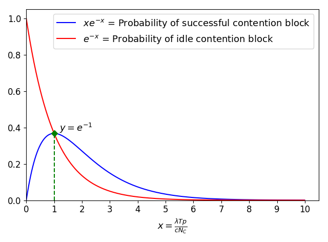
Figure 2: Probability of number of successful and idle blocks

The monotonicity of the probability of an idle block as a function of $p$ then suggests a simple stochastic approximation scheme for adapting $p.$ Let $N_{I}(t)$ denote the number of idle contention blocks observed during the contention phase of frame $t.$ We adapt $p$ as follows.

$$p_{t+1}=\left[p_{t}+\delta_{t}\left(\frac{N_{I}(t)}{cN_{C}}-\frac{1}{e}\right)\right]_{[0,1]}$$ (2)

Here $\delta_{t}$ is the step size, and $[x]_{[0,1]}=\min(1,\max(x,0))$ denotes the projection of $x$ on the interval $[0,1].$ Mathematically, the convergence of $p_{t}$ to $p^{*}$ can be proved under a suitably diminishing step size sequence by standard techniques [13]. However, to make the adaptation robust to (slow) changes in the arrival rate, we take a fixed step size, i.e., $\delta_{t}\equiv\delta.$

Finally, we note that the optimal contention probability depends on the value of $N_{C},$ which the preceding presentation assumes is a constant. Once we describe our adaptation algorithm for $(N_{C},N_{T})$ below, it will be clear how to adjust (2) to account for the dynamic adaptation of $N_{C}.$

IV-B Optimizing the duration of the contention and transmission phases

In this section, we focus on the adaptation of $(N_{C},N_{T})$ based on observed traffic statistics. This is to ensure the optimal balance between the width of the contention phase and the transmission phase so as to maximize the throughput of the system.

We assume that the frame duration $T$ is fixed, and the optimization of $(N_{C},N_{T})$ is to be performed over a pre-defined set $\mathcal{C},$ where

$$\mathcal{C}\subseteq\{(N_{C},N_{T})\in\mathbb{N}\times\mathbb{N}:\ N_{C}+kN_{T}=T\}.$$

Note that $\mathcal{C}$ is a finite set. Our approach is to treat the optimization of $(N_{C},N_{T})$ over $\mathcal{C}$ as a multi-armed bandit (MAB) problem, where the arms correspond to the possible choices of $(N_{C},N_{T}).$

Note that a MAB problem is characterized by a finite set of arms, each arm $i$ being associated with an unknown reward distribution $F_{i}.$ Each time an arm $j$ is played, an independent reward drawn from $F_{j}$ is obtained. The goal is to choose which arm to play in each time slot, seeking to maximize the aggregate reward obtained in the long run. Of course, an oracle that knows the reward distributions of the different arms would simply always play the arm with the highest mean reward. However, since the reward distributions are unknown, MAB algorithms have to estimate the mean reward of each arm by playing it repeatedly. The MAB problem thus captures the classic trade-off between exploration (i.e, playing each arm a large number of times to obtain an accurate estimate of the mean reward), and exploitation (i.e., playing the arm that has so far provided the best mean reward). One classical algorithm for the MAB problem is the Upper Confidence Bound (UCB) algorithm [14]. The regret associated with this algorithm, which is defined as the (average) difference between the aggregate reward obtained by always playing the ‘best’ arm, and the aggregate reward obtained by the algorithm, is known to be $O(\log{N})$ over a horizon of $N$ plays. Note that the UCB plays any suboptimal arm only $O(1/\log{N})$ fraction of the time (over $n$ plays). Moreover, the regret under UCB is near optimal — it can be shown that no online algorithm can have $o(\log{N})$ regret [15].

We apply the UCB algorithm for $(N_{C},N_{T})$ adaptation as follows. The set of arms is $\mathcal{C}.$ Each play of an arm corresponds to operating the corresponding $(N_{C},N_{T})$ setting for $r$ successive frames. The reward is proportional to the number of flows accepted during the play. Specifically, we take the reward to be $\frac{N_{acc}}{cTr},$ where $N_{acc}$ is the total number of accepted flows over the $r$ frames in the play; note that the reward has been normalized to lie in $[0,1].$

To ensure that the rewards are independent across plays, we complete all flows that are active at the end of the $r$ frames in a short sequence of flush frames. No new flows are admitted during these flush frames, which operate with $T/k$ transmission slots. Once all active flows at the end of the play have been completed, the flush frames stop and the next arm is selected.

The UCB algorithm operates as follows. In the beginning, all arms are played once to create an initial estimate. In each subsequent round, we pull the arm that has the highest estimated empirical reward up to that point plus another term that is a decreasing function of the number of times the arm has been played (for example, see [14], [16]). Specifically, let $m_{i,n}$ be the number of times arm $i$ has been played over $n$ plays. Let $r_{n}\in[0,1]$ be the reward we observe at play $n.$ Define $P_{n}\in\mathcal{C}$ be the choice of arm on the $n$th play. The empirical reward estimate of arm $i$ after play $n$ is

$$\hat{\mu}_{i,n}=\frac{\sum_{s=1}^{n}\boldsymbol{1}_{P_{s}=i}r_{s}}{m_{i,n}}.$$

UCB then assigns the following upper confidence bound value to each arm $i$ at each time $n$:

$$\text{UCB}_{i,n}=\hat{\mu}_{i,n}+\sqrt{\frac{2\ln{n}}{m_{i,n}}}.$$

UCB algorithm selects, for play $n+1,$ the arm with the largest upper confidence bound, i.e.,

$$P_{n+1}=\operatornamewithlimits{argmax}\limits_{i\in\mathcal{C}}\text{UCB}_{i,n}.$$

Finally, we note that the contention probability adaptation described earlier is specific to a particular arm. Thus, the $p$-adaptation is performed independently for each arm, when it is played.

V Evaluation

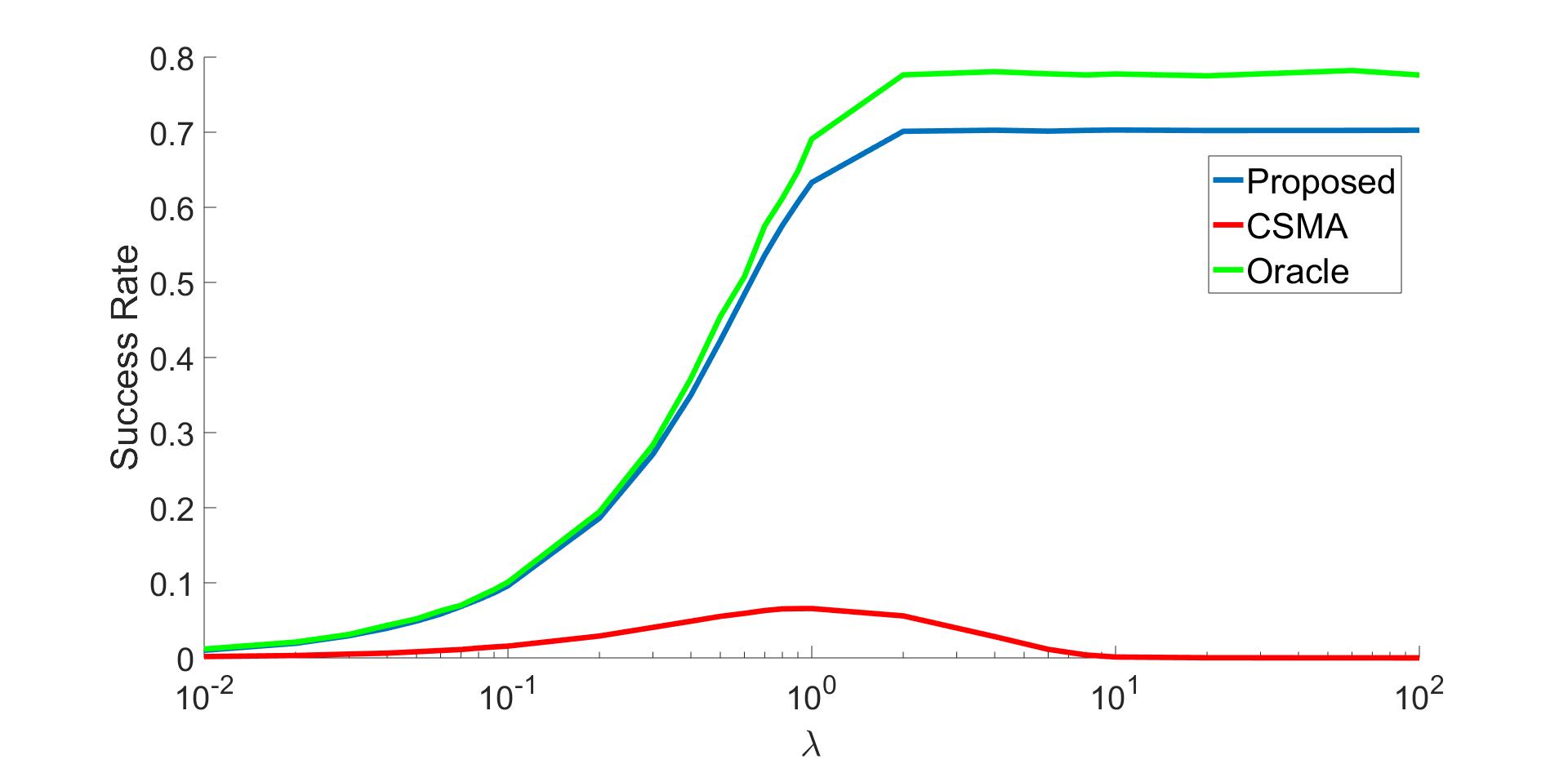
Figure 3: Deterministic load: Throughput v.s. $\lambda$

Figure 4: Deterministic load: Energy v.s. $\lambda$

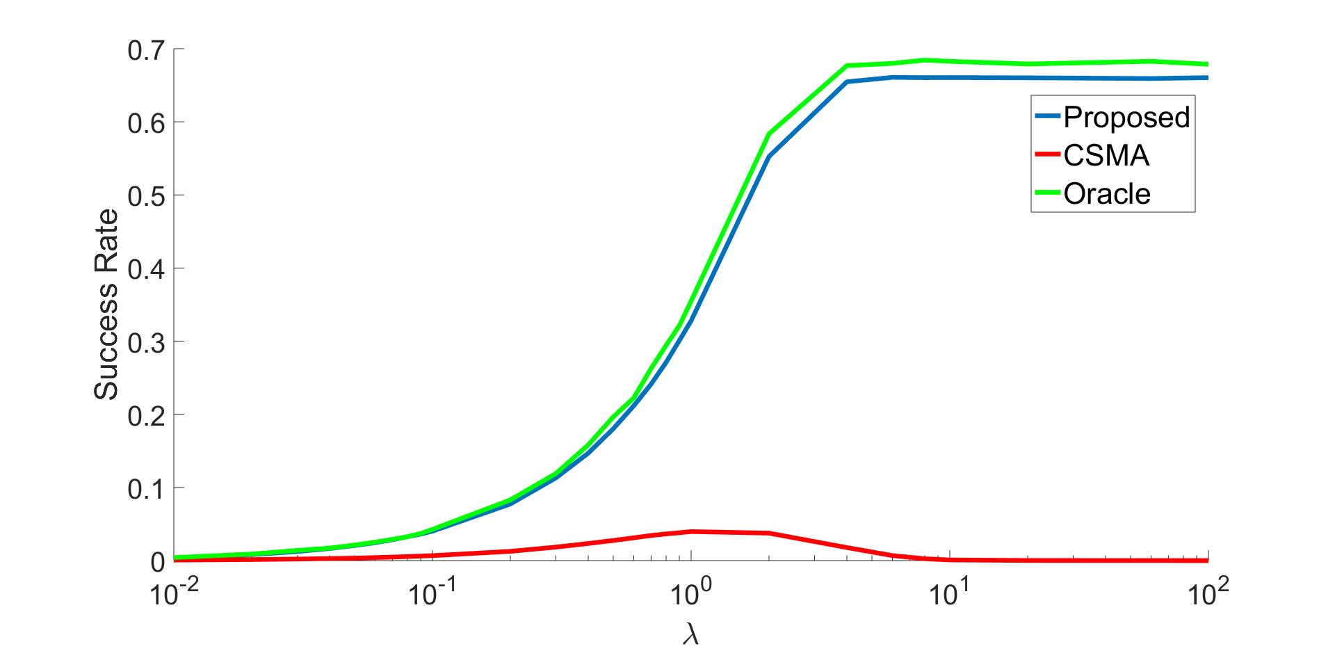
Figure 5: Geometric load: Throughput v.s. $\lambda$

Figure 6: Geometric load: Energy v.s. $\lambda$

The goal of this section is to evaluate the performance of the protocol proposed in the previous sections alongside CSMA/CA via Monte Carlo simulations.

The setting we used for these simulations is the following. We consider 3 channels, i.e., $c=3.$ A single frame is taken to be 50 time units long, with each transmission slot being five times the duration of a contention slot. Thus, the number of transmission slots and contention slots in a frame are constrained by $N_{C}+5N_{T}=50.$ For parameter adaptation, we consider the following possibilities for $(N_{C},N_{T}):$

$$\mathcal{C}=\{(20,6),(15,7),(10,8),(5,9)\}.$$

Each $(N_{C},N_{T})$ configuration is run for $r=50$ frames at a time (as part of a single play of an arm under our MAB formulation).

For the comparison against CSMA/CA, we disregard channel hopping and instead consider a single channel with a flow arrival rate of $\lambda/c.$ (Equivalently, this may be viewed as CSMA/CA running in parallel on $c$ channels, each experiencing $1/c$ fraction of the traffic experienced by the proposed protocol.) We use the exponential backoff model used in WiFi, with initial contention window set to $CW_{\min}=2$ and the maximum contention window set to $CW_{\max}=16.$ Specifically, when a packet experiences a collision, it doubles its contention window $CW$, and picks a uniformly distributed backoff duration $b$ in $\{0,1,\cdots,CW-1\}.$ The next transmission is attempted after the channel has been sensed idle for $b$ time units (recall that one time unit is also the duration of a contention slot in the proposed protocol). The duration of each packet transmission under CSMA/CA is matched to the duration of a transmission slot under the proposed protocol. If a packet suffers three successive collisions, we abort the corresponding flow to maintain stability. Moreover, once a flow misses its deadline under CSMA/CA, it attempts no further transmissions (this limits the overhead on the active flows in the system).

Finally, we evaluate the energy consumption of both protocols by measuring the total transmission time across all flows over the simulation horizon (including transmission during contention slots and transmitted flows in the proposed protocol, and successful as well as collision slots under CSMA/CA), normalized by the number of successful flows. This yields a measure of the energy consumed per successful flow by the system.

We consider two stochastic models for the flow parameters.

Scenario 1: Deterministic load

Here, the load of each flow is deterministic and equal to 3. The slack is taken to be uniformly distributed in the interval $[2,20]$ (the deadline is thus the deterministic load plus the randomly generated slack). Figure 3 depicts the variation of the throughput of the system defined as the rate of successful flows (i.e., number of successful flows over the simulation divided by the simulation time) versus the arrival rate $\lambda$ for (i) the proposed protocol, (ii) an oracle variant of the proposed protocol that always operates the optimal $(p,N_{C},N_{T})$ values, (iii) CSMA/CA. As expected, the throughput of the proposed protocol saturates as the arrival rate grows, given the limited capacity of the system. Moreover, the proposed scheme has a slightly lower saturation throughput compared to the oracle version because of the imperfections in the $p$ adaptation (note that we use a constant step-size), the exploration cost of UCB, as well as the overhead involved in adapting the $(N_{C},N_{T})$ values (the flush frames). In comparison, note that the saturation throughput of CSMA/CA approaches zero as $\lambda$ increases. This is because as the rate of flow arrivals grows, collisions become so prevalent that barely any flows succeed in completing their transmissions before their deadline.

Figure 4 shows the energy consumption per successful flow for all protocols as a function of $\lambda,$ on a log-log scale. As we see, the energy efficiency of the proposed protocol remains steady with increasing $\lambda,$ since our reservation-based MAC only ‘wastes’ energy during the contention phase. Moreover, note that the energy efficiency closely matches the oracle-based benchmark. In contrast, CSMA/CA has an energy per successful flow that grows unboundedly with the arrival rate, due to the steady energy consumption but dwindling throughput.

Scenario 2: Random load

Next, we consider the case where the load of each flow is geometrically distributed with a mean value of 1.25, with the slack distribution unchanged. Figures 5 and 6 depict, respectively, the throughput and energy (on a log scale) per successful flow for the same protocols. We see the same patterns as the deterministic load case.

We conclude this section by noting that the proposed protocol outperforms CSMA/CA with respect to throughput (equivalently, QoS-compliance) as well as energy efficiency. This is particularly true in heavy traffic, where the number of nodes attempting to access the channel at any time is large (different from the settings in which WiFi is presently deployed), when the overhead associated with the completely distributed scheduling by CSMA/CA becomes prohibitive.

VI Concluding remarks

In this paper, we propose a reservation-based MAC framework for IoT/M2M applications, where flows are scheduled centrally in a deadline-aware manner by a central master node, and MAC parameters are adapted dynamically based on the statistics of the observed traffic. We demonstrate that such a MAC outperforms CSMA/CA when the number of connected devices becomes large, as is projected in the IoT regime.

Note that the proposed framework can co-exist alongside conventional WiFi — WiFi being used to connect a few user-operated (high-bandwidth) devices, and the proposed reservation-based MAC being used to connect the (large number of) IoT devices.

Future work will focus on (i) proving the throughput optimality of the proposed schemes, (ii) extending to flows that are periodic in nature, and (iii) generalizing to the case of multiple interfering networks, each with their own master node, where the masters dynamically allocate channels among themselves based on their observed congestion as well as interference constraints.

References

- [1] J. F. Kurose and K. W. Ross, Computer Networking: A top-down approach: international edition. Pearson Higher Ed, 2013.
- [2] D. De Guglielmo, S. Brienza, and G. Anastasi, “IEEE 802.15.4e: A survey,” Computer Communications, vol. 88, pp. 1–24, 2016.
- [3] M. M. Mohiuddin, I. Adithyan, and P. Rajalakshmi, “EEDF-MAC: An energy efficient mac protocol for wireless sensor networks,” in 2013 International Conference on Advances in Computing, Communications and Informatics (ICACCI), 2013.
- [4] M. L. Dertouzos and A. K. Mok, “Multiprocessor online scheduling of hard-real-time tasks,” IEEE Transactions on software engineering, vol. 15, no. 12, pp. 1497–1506, 1989.
- [5] O. Chipara, C. Wu, C. Lu, and W. Griswold, “Interference-aware real-time flow scheduling for wireless sensor networks,” in 2011 23rd Euromicro Conference on Real-Time Systems, 2011.
- [6] C. Zhu and M. S. Corson, “A five-phase reservation protocol (FPRP) for mobile ad hoc networks,” in Proceedings. IEEE INFOCOM ’98, 1998.
- [7] A. Tinka, T. Watteyne, K. S. Pister, and A. M. Bayen, “A decentralized scheduling algorithm for time synchronized channel hopping,” EAI Endorsed Transactions on Mobile Communications and Applications, vol. 1, no. 1, pp. 1–13, 2011.
- [8] M. Harchol-Balter, Performance modeling and design of computer systems: queueing theory in action. Cambridge University Press, 2013.
- [9] D. P. Bertsekas and R. G. Gallager, Data networks. Prentice-Hall International New Jersey, 1992.
- [10] P. Brucker, Scheduling algorithms. Springer, 2007.
- [11] C. Qian, H. Ngan, Y. Liu, and L. M. Ni, “Cardinality estimation for large-scale rfid systems,” IEEE Transactions on parallel and distributed systems, vol. 22, no. 9, pp. 1441–1454, 2011.
- [12] S. Kadam, C. S. Raut, and G. S. Kasbekar, “Fast node cardinality estimation and cognitive mac protocol design for heterogeneous m2m networks,” in IEEE GLOBECOM, 2017.
- [13] V. S. Borkar, Stochastic approximation: A dynamical systems viewpoint. Cambridge University Press, 2009.
- [14] G. Burtini, J. Loeppky, and R. Lawrence, “A survey of online experiment design with the stochastic multi-armed bandit,” arXiv preprint arXiv:1510.00757, 2015.
- [15] T. L. Lai and H. Robbins, “Asymptotically efficient adaptive allocation rules,” Advances in applied mathematics, vol. 6, no. 1, pp. 4–22, 1985.
- [16] P. Auer, N. Cesa-Bianchi, and P. Fischer, “Finite-time analysis of the multiarmed bandit problem,” Machine learning, vol. 47, no. 2-3, pp. 235–256, 2002.