Photonic topological insulators induced by non-Hermitian disorders in a coupled-cavity array

Abstract

Recent studies of disorder or non-Hermiticity induced topological insulators inject new ingredients for engineering topological matter. Here we consider the effect of purely non-Hermitian disorders, a combination of these two ingredients, in a 1D coupled-cavity array with disordered gain and loss. Topological photonic states can be induced by increasing gain-loss disorder strength with topological invariants carried by localized states in the complex bulk spectra. The system showcases rich phase diagrams and distinct topological states from Hermitian disorders. The non-Hermitian critical behavior is characterized by the biorthogonal localization length of zero-energy edge modes, which diverges at the critical transition point and establishes the bulk-edge correspondence. Furthermore, we show that the bulk topology may be experimentally accessed by measuring the biorthogonal chiral displacement, which can be extracted from a proper Ramsey interferometer that works in both clean and disordered regions. The proposed coupled-cavity photonic setup relies on techniques that have been experimentally demonstrated, and thus provides a feasible route towards exploring such non-Hermitian disorder driven topological insulators.

I Introduction

Topological insulators (TIs), exotic states of matter exhibiting gapless edge modes determined by quantized features of their bulk xiao2010berry ; hasan2010colloquium ; qi2011topological ; RevModPhys.88.035005 , have been widely studied in various systems PhysRevLett.95.146802 ; Bernevig2006quantum ; Konig2007quantum ; PhysRevLett.111.185301 ; PhysRevLett.111.185302 ; Jotzu2014Experimental ; Goldman2016topological ; Cooper2018topological ; haldane2008possible ; hafezi2011robust ; fang2012realizing ; lu2014topological ; kraus2012topological ; Hafezi2013imaging ; Ozawa2018Topological ; Ma2019Topological . Recently, the concept of TIs has been generalized to open quantum systems characterized by non-Hermitian Hamiltonians Rept.Prog.Phys.70.947 , which may exhibit unique properties without Hermitian counterparts Eur.Phys.J.Spec.Top227 . The experimental advances in controlling gain and loss in photonic systems  PhysRevLett.100.103904 ; PhysRevLett.115.200402 ; PhysRevLett.115.040402 ; NatMater16433 ; Photon.Rev.6.A51 ; Nature488.167 ; PhysRevLett.113.053604 ; Science346Loss ; Zhao2018topological ; PhysRevLett.120.113901 ; Bandres2018Topological ; St-Jean2017Lasing , as well as other systems such as atomic and electric circuit systems Muller2012Engineered ; Ashida2017Parity ; PhysRevLett.121.026403 ; arXiv1802.00443 ; PhysRevB.98.035141 ; PhysRevLett.118.045701 ; arXiv1608.05061 ; arXiv1811.06046 ; arXiv1907.11562 provide powerful tools for studying non-Hermitian topological phases. Beside new topological invariants PhysRevB.84.205128 ; PhysRevA.93.062101 ; PhysRevLett.121.026808 ; PhysRevLett.116.133903 ; PhysRevLett.121.136802 ; PhysRevLett.121.213902 ; PhysRevLett.121.086803 ; PhysRevX.8.031079 , the unique features (e.g., complex eigenvalues, eigenstate biorthonormality, exceptional points, etc.) of non-Hermitian systems can lead to novel topological phenomena, such as the non-Hermitian skin effects, exceptional rings and bulk Fermi arcs, with bulk-edge correspondence very different from the Hermitian systems PhysRevLett.116.133903 ; PhysRevLett.121.136802 ; PhysRevLett.121.213902 ; PhysRevLett.121.086803 ; PhysRevX.8.031079 ; PhysRevLett.121.026808 ; arXiv1808.09541 ; PhysRevB.97.045106 ; PhysRevLett.118.040401 ; PhysRevLett.120.146402 ; Xiong2018why ; Science359Observation ; arXiv1804.04676 ; PhysRevB.99.081103 ; arXiv1812.02011 ; arXiv1809.02125 ; arXiv1902.07217 ; PhysRevB.100.075403 ; arXiv1905.07109 ; PhysRevLett.123.170401 ; PhysRevLett.123.246801 ; PhysRevB.100.045141 ; arXiv1912.04024 ; arXiv1910.03229 ; PhysRevB.97.075128 ; arXiv1806.10268 ; ncommss41467 ; arXiv1907.12566 .

A key property of TIs (either Hermitian or non-Hermitian) is their robustness against weak disorders through the topological protection xiao2010berry ; hasan2010colloquium ; qi2011topological . For sufficiently strong disorders, the system becomes topologically trivial through Anderson localization PhysRev.109.1492 , accompanied by the unwinding of the bulk topology PhysRevB.50.3799 ; PhysRevLett.98.076802 ; PhysRevLett.97.036808 ; PhysRevLett.105.115501 . In this context, the prediction of the reverse process that non-trivial topology can be induced, rather than inhibited, by the addition of disorder to a trivial insulator was surprising PhysRevLett.102.136806 . The disorder-induced topological states, known as topological Anderson insulators (TAIs), can support robust topological invariants carried entirely by localized states. They have attracted many theoretical studies PhysRevB.80.165316 ; PhysRevLett.103.196805 ; PhysRevLett.105.216601 ; PhysRevLett.112.206602 ; PhysRevLett.114.056801 ; PhysRevLett.119.183901 ; PhysRevLett.113.046802 ; PhysRevB.89.224203 and been experimentally demonstrated in 1D synthetic atomic wires science.aat3406 and 2D photonic lattices Nature560.461 .

So far the studies of TAIs have been mainly focused on Hermitian disorders, where a major challenge for their implementation is the average of large numbers of disorder configurations due to the non-tunability of the fabricated devices. In contrast, non-Hermitian disorders through gain and loss can be tuned through additional pumping in photonic system and different disorder configurations can be realized on a single optical device. Therefore, two natural questions arise: Can novel topological states be induced by purely non-Hermitian disorders? If so, what are the criticality and bulk-edge correspondence for general non-Hermitian TAIs? Furthermore, experimental schemes for probing non-Hermitian bulk topology are highly desirable, but still lacked even for clean systems.

In this paper, we address these important issues by considering a 1D chiral symmetric lattice in the presence of purely non-Hermitian disorders (e.g., disordered gain and loss), and develop feasible experimental implementations based on photons in coupled cavity arrays. Our main results are: (i) Photonic topological insulators can be induced solely by gain-loss disorders with topological winding number carried by localized states in the (complex) bulk spectra. Such non-Hermitian TAIs reveal richer phase diagrams and distinct topological states compared to the Hermitian one. (ii) We examine the general critical behaviors of non-Hermitian TAIs by deriving the biorthogonal localization length of the zero edge mode, which diverges at the critical transition point, establishing the bulk-edge correspondence. (iii) We propose to experimentally probe the bulk topology by measuring the biorthogonal chiral displacement $\mathcal{C}$, which converges to the winding number under time-averaging [in the parity-time (PT) symmetric region]. We show how $\mathcal{C}$ can be extracted using a proper Ramsey interferometer, which provides the first realistic method to measure the topological invariants of non-Hermitian systems and works for both disorder and clean regions.

II Model

We consider a disordered non-Hermitian Su-Schrieffer-Heeger (SSH) PhysRevLett.42.1698 model with a chiral or sublattice symmetry, as shown in Fig. 1a. The tight-binding Hamiltonian reads

$$H = \sum_{n}\big{[}c_{n}^{\dagger}(m_{n}\sigma^{x}-i\gamma_{n}\sigma^{y})c_{n}$$ (1)

$$+J^{+}_{n}c_{n}^{\dagger}\sigma^{+}c_{n+1}+J^{-}_{n}c_{n+1}^{\dagger}\sigma^{-}c_{n}\big{]}$$

with $c_{n}^{\dagger}=(c_{n,A}^{\dagger},c_{n,B}^{\dagger})$ the particle creation operator of sites $A$ and $B$ in the unit cell $n$ ($n\in[-N,N-1]$), and $\sigma^{\pm}=\frac{1}{2}(\sigma^{x}\pm i\sigma^{y})$, $J^{\pm}_{n}=J_{n}\pm\kappa_{n}$. $m_{n}$ and $J_{n}$ are the Hermitian parts of the intra- and inter-cell tunnelings, which are set to be uniform $m_{n}=m$ and $J_{n}=J$. The purely non-Hermitian disorders are given by the anti-Hermitian parts $\gamma_{n}$ and $\kappa_{n}$ (corresponding to gain and loss during tunnelings), which are independently and randomly generated numbers drawn from the uniform distributions $[\gamma_{\text{b}}-\frac{W_{\gamma}}{2},\gamma_{\text{b}}+\frac{W_{\gamma}}{2}]$ and $[\kappa_{\text{b}}-\frac{W_{\kappa}}{2},\kappa_{\text{b}}+\frac{W_{\kappa}}{2}]$, respectively. The biases $\gamma_{\text{b}}$ and $\kappa_{\text{b}}$ correspond to the periodic non-Hermiticities. The model preserves the chiral symmetry $\Gamma H\Gamma^{-1}=-H$ ($\Gamma$ flips the sign of particles on sites $B$), and thus the eigenvalues appear in pairs $(E,-E)$. The system also preserves a hidden PT symmetry (see Appendix A), which may be broken by strong non-Hermitian disorders. Hereafter, we will set $J=1$ as the energy unit and focus on $\gamma_{\text{b}}=0$ unless otherwise noted.

The above disordered non-Hermitian SSH model can be realized using photons in coupled optical cavities PhysRevLett.120.113901 ; St-Jean2017Lasing ; Bandres2018Topological ; Zhao2018topological ; Sci.Rep.5.13376 ; science.aba8996 . Shown in Fig. 1b is the proposed photonic circuit, where site micro-ring cavities are evanescently coupled to their nearest neighbors using a set of auxiliary micro-rings, each of which can be controlled independently. The non-Hermitian (asymmetric) tunnelings can be realized by adding gain and loss to the two arms of the auxiliary micro-rings, respectively Bandres2018Topological ; Zhao2018topological ; Sci.Rep.5.13376 ; science.aba8996 . We first consider the clockwise modes only, for either leftward or rightward tunnelings, photons in the micro-ring cavities use different arms of the auxiliary micro-rings with opposite non-Hermiticities, leading to exactly the Hamiltonian $H$ in Eq. 1 (see Appendix B for more details). Similarly, the counterclockwise modes are characterized by Hamiltonian $H^{{\dagger}}$ which will be used to probe the bulk topology, as we discussed later.

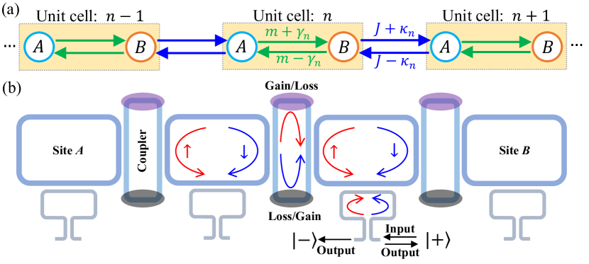
Figure 1: (a) Lattice representation of the generalized SSH Hamiltonian in Eq. 1, with purely non-Hermitian disorders $\gamma_{n}$, $\kappa_{n}$. (b) Experimental implementation of the lattice model shown in (a) using coupled arrays of cavities.

III Results

Phase diagrams. For disordered systems, the topological invariant should be defined in real space. Even in the clean limit, the real-space topological invariant would be a natural choice to characterize non-Hermitian systems due to their extreme sensitivity to boundary conditions (open-boundary spectra are very different from the periodic ones), and the topology is encoded in the spectra with open-boundary condition where protected edge states can exist.

We generalize the real-space winding number PhysRevLett.113.046802 for a non-Hermitian chiral-symmetric system as (see Appendix C)

$$\nu = \frac{1}{4}\mathcal{T}\{Q\Gamma[\hat{X},Q]+Q^{\dagger}\Gamma[\hat{X},Q^{\dagger}]\},$$ (2)

where $\hat{X}$ is the unit-cell position operator, $\mathcal{T}$ is the trace per volume and $Q=P_{+}-P_{-}$ is the flattened Hamiltonian with $P_{\pm}=\pm\sum_{j}|\Psi^{R}_{j,\pm}\rangle\langle\Psi^{L}_{j,\pm}|$. $|\Psi^{R,L}_{j,\pm}\rangle$ satisfy $H|\Psi^{R}_{j,\pm}\rangle=E_{j,\pm}|\Psi^{R}_{j,\pm}\rangle$ and $H^{\dagger}|\Psi^{L}_{j,\pm}\rangle=E^{*}_{j,\pm}|\Psi^{L}_{j,\pm}\rangle$, with chiral-symmetric pairs $E_{j,+}=-E_{j,-}$ and $|\Psi^{R,L}_{j,\mp}\rangle=\Gamma|\Psi^{R,L}_{j,\pm}\rangle$. The choice of occupied bands $E_{j,-}$ is very flexible and different choices lead to the same winding number. Different from Hermitian TAIs, here both $Q$ and $Q^{\dagger}$ ($Q\neq Q^{\dagger}$) are included in the definition of the winding number to guarantee a real-valued invariant.

We first consider stronger intra-cell disorders $W_{\gamma}=8W_{\kappa}=W$. Fig. 2a shows the phase diagram in the $W$-$m$ plane with $\kappa_{\text{b}}=0.1$. At $W=0$ (no disorder), the system is in topological phase with $\nu=1$ for $m^{2}<|1-\kappa_{\text{b}}^{2}|$ PhysRevLett.121.086803 . For a small $W$, the disorders tend to weaken the intra-cell couplings, leading to the enlargement of the topological region as $W$ increases. That is, trivial system becomes topological through the addition of non-Hermitian disorders, as shown in Fig. 2b with $m=1.1$. The winding number fluctuates strongly near the phase boundary and the fluctuations are more significant for stronger non-Hermiticities (see Appendix C). In the $W\rightarrow\infty$ limit, the intra-cell couplings become dominant and the system must become trivial ($\nu=0$) for all $m$ and $\kappa_{\text{b}}$. In Fig. 2c, we plot the phase diagram as a function of $\kappa_{\text{b}}$ for $m=1.1$. The area of disorder-induced topological phase shrinks to zero as $|\kappa_{\text{b}}|$ increases, leading to a topological island in the $W$-$\kappa_{\text{b}}$ plane. In the strong $|\kappa_{\text{b}}|$ limit, the system enters the topological phase again as the inter-cell couplings becomes dominant. Such phase diagrams are unique for non-Hermitian disorders, since the interplay between Hermitian and non-Hermitian tunnelings tends to weaken each other and the effective two-site coupling reaches its minimum when they are comparable.

As $W$ increases, the gap at $E=0$ closes prior to the phase transition to $\nu=0$ and $\nu=1$ for $m^{2}<|1-\kappa_{\text{b}}^{2}|$ and $m^{2}>|1-\kappa_{\text{b}}^{2}|$, respectively (see Appendix A). The stripped lines in Figs. 2a-c are the PT-symmetry breaking curves, indicating the topological phase is unaffected by the disorder-driven PT-symmetry breaking or band gap closing, and $\nu$ remains robust for much stronger disorders. For dominant inter-cell disorders $W_{\kappa}\gg W_{\gamma}$, the phase diagram can be obtained similarly, where the system becomes topological, rather than trivial, in the $W_{\kappa}\rightarrow\infty$ limit.

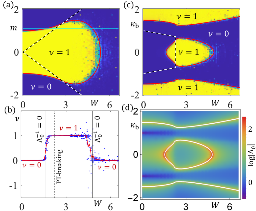
Figure 2: (a) Phase diagram in the $m$-$W$ plane with $\kappa_{\text{b}}=0.1$. The winding number (shown by color scale) is averaged over 10 disorder configurations for an extremely large $N=300$. Red solid line is the analytic critical boundary and stripped line is the PT-symmetry breaking curve. (b) The winding number along the horizontal line in (a) with $m=1.1$. The un-averaged data for 10 disorder configurations are shown by the scattered blue points and the average by the red solid line. (c) Phase diagram in the $\kappa_{\text{b}}$-$W$ plane with $m=1.1$. Other parameters are the same as in (a). (d) The analytic zero-mode Biorthogonal localization length corresponding to the phase diagram in (c). $W_{\gamma}=8W_{\kappa}=W$ in all plots.

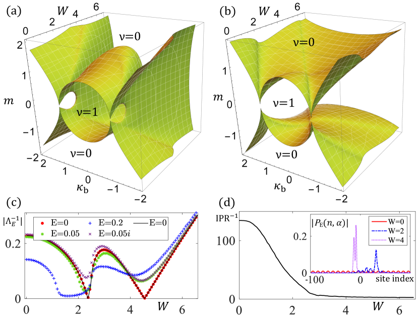
Figure 3: (a) and (b) Phase diagrams in the three-dimensional parameter space ($m$, $\kappa_{b}$, $W$) based on delocalized critical surface with $W=W_{\gamma}=8W_{\kappa}$ and $W=W_{\kappa}=8W_{\gamma}$, respectively. (c) The biorthogonal localization lengths versus disorder at different energies. Data points are obtained by numerical transfer matrix analysis and solid line is the analytic result for $E=0$. The transfer matrix was iterated $10^{6\sim 8}$ times. (d) Biorthogonal IPR averaged over all states and 100 disorder configurations with $N=50$. The inset shows the biorthogonal density distribution $P_{E}(n,\alpha)$ around $\text{Re}[E]=-1.5$. The site index is $2n+\alpha$. Other parameters in (c) and (d): $m=1.25$, $\kappa_{\text{b}}=0.1$ and $W=W_{\gamma}=8W_{\kappa}$.

Biorthogonal criticality. For both clean and disordered Hermitian systems PhysRevLett.113.046802 , the edge states (i.e., zero-energy modes) become delocalized at the topological critical point RevModPhys.88.035005 . Different from Hermitian systems, here the left and right eigenstates are inequivalent and may suffer skin effects, both of which need be taken into account to characterize the criticality (see Appendix D). We examine such biorthogonal criticality by deriving the analytic formula of the zero-mode localization length, which enables us to identify the topological phase boundary. The zero modes of the eigenequations $H|\Psi_{0}^{R}\rangle=0$ and $H^{{\dagger}}|\Psi_{0}^{L}\rangle=0$ can be solved exactly, from which we obtain the biorthogonal distributions $P(n,\alpha)=\langle\Psi_{0}^{L}(n,\alpha)|\Psi_{0}^{R}(n,\alpha)\rangle$ as

$$P(n,\alpha)=P(0,\alpha)\prod_{n^{\prime}=0}^{n-1}\left(\frac{m-\gamma_{n^{\prime}+\alpha}^{2}}{1-\kappa_{n^{\prime}}^{2}}\right)^{\eta_{\alpha}}.$$ (3)

Here $\alpha=0,1$ and $\eta_{\alpha}=\pm$ correspond to sublattice sites $A$ and $B$, respectively. The biorthogonal localization lengths are defined as $\Lambda_{\alpha}^{-1}=-\frac{1}{2}\lim_{n\rightarrow\infty}\frac{1}{n}\ln|\frac{P(n,\alpha)}{P(0,\alpha)}|$, which do not suffer skin effects and satisfy $\Lambda_{0}^{-1}=-\Lambda_{1}^{-1}$. $\Lambda_{0}$ as a function of $m$, $W_{\gamma}$, $W_{\kappa}$, $\gamma_{\text{b}}$ and $\kappa_{\text{b}}$ can be obtained after ensemble average (the explicit expression can be found in Appendix D), and the critical exponent is 1. Interestingly, $\Lambda_{0}$ at $\gamma_{\text{b}}=\kappa_{\text{b}}=0$ is exactly the same as that of the Hermitian system studied in PhysRevLett.113.046802 , though the characterization is different.

The bulk $\nu$ and edge $\Lambda_{0}$ quantities establish the generalized bulk-edge correspondence for the non-Hermitian TAIs. In the topological (trivial) phase with $\nu=1$ ($\nu=0$), we have $(-1)^{\alpha}\Lambda_{\alpha}>0$ [$(-1)^{\alpha}\Lambda_{\alpha}<0$]. Recall that the lattice starts (ends) by a site $A$ (B) at the left (right) boundary, $(-1)^{\alpha}\Lambda_{\alpha}>0$ indicates one zero mode at each boundary. The topological phase transition occurs at the delocalized critical surface where the biorthogonal localization length $\Lambda_{0}$ diverges (i.e., $\Lambda_{0}^{-1}$ crosses zero). Fig. 2d shows the corresponding $\Lambda_{0}$ of the phase diagram in Fig. 2c. In Figs. 3a and 3b, the exact phase diagrams in the whole parameter space $(m,\kappa_{\text{b}},W)$ are plotted for $\Lambda_{0}^{-1}=0$ with dominant intra-cell ($W=W_{\gamma}=8W_{\kappa}$) and inter-cell ($W=W_{\kappa}=8W_{\gamma}$) disorders, respectively (for other disorder configurations see Appendix D). The non-Hermitian TAIs support richer phase diagrams and topological phenomena going beyond Hermitian TAIs. In Fig. 3a, the topological regions at small and large $|\kappa_{\text{b}}|$ are connected by two holes, whose size is proportional to $W_{\kappa}$. In Fig. 3b, the two trivial regions at large $m$ are separated by the topological region around $m=0$. These results are in agreement with the phase diagrams predicted by $\nu$ (see Figs. 2a-c).

The critical behavior is characterized only by the zero modes, all states with $E\neq 0$ are localized in every instance with disorders. Using a numerical analysis of the transfer matrix Z.Phys.B.53 ; PhysRevB.29.3111 for both $H$ and $H^{\dagger}$ (see Appendix D), we calculate the biorthogonal localization lengths as functions of disorder strength and confirm the localization behavior of the bulk states (see Fig. 3c). Fig. 3d shows the disorder-averaged inverse participation ratio (IPR) RevModPhys.80.1355 obtained from the biorthogonal density distributions (see Appendix D), which also imply the localization of the entire bulk (larger IPR corresponds to stronger localization). We emphasize that, the biorthogonal density distributions and localization lengths do not suffer skin effects which may exist in the left/right eigenstates.

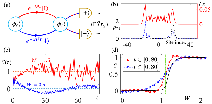
Figure 4: (a) Ramsey interferometer for measuring $\mathcal{C}$. (b) Density distributions of $|\phi_{t}\rangle$ at $t=10$ and $W=1.5$. $\rho_{x}$, $\rho_{\uparrow}$ and $\rho_{\downarrow}$ are shown by the solid, dashed and dotted lines respectively. (c) Dynamics of $\mathcal{C}(t)$ for topological and trivial phases at different $W$. The dashed lines are the time-averaged value $\bar{\mathcal{C}}$ in the interval $t\in[0,80]$. (d) Evolution of $\bar{\mathcal{C}}$ with disorder for different averaging time intervals. The black solid line is the corresponding winding number $\nu$. All results in (b)-(d) are averaged over 100 disorder configurations with $m=1.05$, $\gamma_{\text{b}}=0$, $W=W_{\gamma}=8W_{\kappa}$. $N$ is chosen such that the wave functions do not reach the boundary during the evolution.

Probing the topology. For disordered system, the zero edge modes, usually embedded in the gapless bulk spectra, are difficult to detect; not to mention that the non-Hermitian (left or right) bulk states may also be localized near the edges due to skin effects. Determining the bulk winding from Eq. 2 requires the measurement of all possible eigenstates, which is also hard to perform. Another way to access the topological invariant is to monitor the dynamical response of photons initially prepared on site $A$ of unit-cell $n=0$ (denoted as $|0_{A}\rangle$) and measure the mean chiral displacement science.aat3406 ; ncomms15516 . Different from Hermitian models, here the time evolution under $H$ is not unitary, and the usual scheme no longer works. To overcome this difficulty, we introduce the biorthogonal chiral displacement

$$\mathcal{C}(t)=\langle L(t)|\Gamma\hat{X}|R(t)\rangle+h.c.,$$ (4)

which includes the dynamics of both $H$ and $H^{\dagger}$, with $|R(t)\rangle=\exp(-iHt)|0_{A}\rangle$, $|L(t)\rangle=\exp(-iH^{\dagger}t)|0_{A}\rangle$ and $\langle L(t)|R(t)\rangle=1$. We find in the PT-symmetric region (i.e., real-spectrum region), $\mathcal{C}(t)$ converges to the winding number $\nu$ upon sufficient time- and disorder-averaging $\bar{\mathcal{C}}=\langle\mathcal{C}(t)\rangle$ (see Appendix E). In the clean limit, the disorder-averaging is unnecessary.

We now propose a method to measure the biorthogonal chiral displacement using proper Ramsey interferometer sequences as shown in Fig. 4a. First we introduce an additional pseudospin degree of freedom, and prepare the photons in state $|\phi_{0}\rangle=|+\rangle|0_{A}\rangle$ with pseudospin state $|\pm\rangle=\frac{1}{\sqrt{2}}(\left|\uparrow\right\rangle\pm\left|\uparrow\right\rangle)$. Then we engineer the dissipations such that the dynamics of photons in the two pseudospin states $\left|\uparrow\right\rangle$ and $\left|\downarrow\right\rangle$ are governed by $H$ and $H^{{\dagger}}$ respectively. The total Hamiltonian reads

$$H_{\text{probe}}=H\otimes\left|\uparrow\right\rangle\left\langle\uparrow\right|+H^{{\dagger}}\otimes\left|\downarrow\right\rangle\left\langle\downarrow\right|.$$ (5)

After an evolution interval $t$, we measure the chiral displacement in basis $|\pm\rangle$, and the outcome gives $\mathcal{C}(t)=\langle\phi_{t}|2\Gamma\hat{X}\tau^{x}|\phi_{t}\rangle,$ with $|\phi_{t}\rangle=\exp(-iH_{\text{probe}}t)|\phi_{0}\rangle$ and $\tau^{x}$ the Pauli matrix in the pseudospin basis.

The disorder driven topological phase transition may occur before the PT-symmetry breaking (see Fig. 2a), and thus can be probed by the dynamical response. In Fig. 4b, we plot the typical (disorder-averaged) photonic density distributions $\rho_{s}=\langle\phi_{t}(n,\alpha)|\tau^{s}|\phi_{t}(n,\alpha)\rangle$ in different pseudospin basis ($\tau^{\uparrow}=\left|\uparrow\right\rangle\left\langle\uparrow\right|$). The pseudospin up and pseudospin down densities may be amplified with strong asymmetric distributions away from $n=0$ due to the non-Hermitian (i.e., non-reciprocity) tunnelings. However, their interference density pattern $\rho_{x}$, almost symmetrically distributed around $n=0$, remains finite and normalized [$\sum_{n,\alpha}\rho_{x}(n,\alpha)=1$]. Fig. 4c shows the disorder-averaged dynamics of $\mathcal{C}(t)$ with different disorder strengths, which converge to $0$ and $1$ upon time-averaging for trivial and topological phases, respectively. The dependence of $\bar{\mathcal{C}}$ on the strength of applied disorder is shown in Fig. 4d, which changes from $\bar{\mathcal{C}}=0$ to $\bar{\mathcal{C}}=1$ across the disorder driven topological phase transition.

As shown in Fig. 1b, for either leftward or rightward tunnelings, the clockwise mode and counterclockwise mode in the micro-ring cavity use different arms of the coupler with opposite non-Hermiticities, leading to exactly the Hamiltonian $H_{\text{probe}}$ in Eq. 5 (see Appendix B), where clockwise and counterclockwise modes play the role of pseudospin degrees of freedom. To measure the Ramsey interference, we propose to couple each cavity with an input-output waveguide hafezi2011robust ; PhysRevLett.120.113901 , as shown in Fig. 1b. The waveguide is arranged as a Sagnac interferometer so that the initial state $|\phi_{0}\rangle$ can be prepared by a narrow optical input pulse applying to site $A$ at $n=0$, and the two output ports measure the photonic pseudospin states in the basis $|+\rangle$ and $|-\rangle$, respectively (see Appendix B).

IV Discussion and Conclusion

In summary, we proposed and characterized non-Hermitian photonic TAIs induced solely by gain/loss disorders which showcase richer phase diagrams and distinct topological states compared to Hermitian TAIs, and developed the first realistic method to probe their topological invariants. Though we focused on the photonic systems based on coupled-cavity arrays, it is possible to generalize our study to other systems such as cold atoms in optical lattices and microwaves in electric circuits, where the non-Hermitian tunnelings can be realized by Raman couplings with lossy atomic levels arXiv1608.05061 ; PhysRevX.8.031079 ; arXiv1810.04067 and circuit amplifiers/resistances as realized in recent experiment arXiv1907.11562 . Moreover, it will be exciting to study the interaction effects and its interplay with non-Hermitian disorders, where non-trivial many-body topological ground states or many-body localization may exist (Recent studies suggest even periodic non-Hermiticity could significantly alert the localization properties PhysRevLett.77.570 ; PhysRevB.92.195107 ; PhysRevA.91.033815 ; PhysRevA.95.062118 ; PhysRevLett.116.237203 ; PhysRevLett.123.090603 ).

Our biorthogonal topological characterizations may be useful for exploring other disordered non-Hermitian systems, and is possible to be generalized to interacting many-body topological states (see Appendix F). The proposed Ramsey interferometer allows the coherent extraction of information from both right and left eigenstates, which may have potential applications in probing the topology of various non-Hermitian systems. Previous studies on non-Hermitian TAIs mainly focused on strong Hermitian disorders in the PT-symmetric region arXiv1908.01172 , where topological characterization does not apply to general non-Hermitian TAIs like our model; in addition, the critical behavior (e.g., the biorthogonal localization length) for general non-Hermitian TAIs, the probing scheme based on chiral displacement and its Ramsey-interferometer implementation, the coupled-cavity experimental realization were not considered. Our work offers a new route towards exploring novel photonic topological insulators and rich phenomena going beyond Hermitian systems and paves the way for characterizing and probing non-Hermitian topological states.

V Appendix A: Hidden PT symmetry

As we mentioned in the main text, the system obeys a hidden PT symmetry. To see this, we first apply a unitary rotation in the sublattice space $c_{n}\rightarrow\widetilde{c}_{n}=\exp(i\frac{\pi}{4}\sigma^{x})c_{n}$, and rewrite the Hamiltonian as

$$H=\sum_{n}\big{[}\widetilde{c}_{n}^{\dagger}(m\sigma^{x}-i\gamma_{n}\sigma^{z})\widetilde{c}_{n}+(J+\kappa_{n})\widetilde{c}_{n}^{\dagger}\frac{\sigma_{x}+i\sigma_{z}}{2}\widetilde{c}_{n+1}+(J-\kappa_{n})\widetilde{c}_{n+1}^{\dagger}\frac{\sigma_{x}-i\sigma_{z}}{2}\widetilde{c}_{n}\big{]}.$$ (A1)

Then, we define the parity and time-reversal operators in the basis $\widetilde{c}_{n}$ as $\mathcal{P}=\sigma_{x}$ and $\mathcal{T}=\mathcal{K}$ (with $\mathcal{K}$ denoting complex conjugation), respectively. Therefore, the Hamiltonian preserves the PT symmetry as $\mathcal{PT}H(\mathcal{PT})^{-1}=H$. The lattice representation of Eq. A1 is shown in Fig. A1(a). The parity operator corresponds to the reflection with respect to the horizontal dashed line, which exchanges sublattice sites $A$ and $B$. We find that the system is PT-symmetric in the weak non-Hermitian region when both $|\gamma_{n}|<|m|$ and $|\kappa_{n}|<|J|$ are satisfied for all $n$ (i.e., $W_{\gamma}+|\gamma_{\text{b}}|<|m|$ and $W_{\kappa}+|\kappa_{\text{b}}|<|J|$). Otherwise, the PT-symmetry is spontaneously broken. The spectrum is real in the PT-symmetric region and becomes complex in the PT-symmetry breaking region. The typical band structure is shown in Figs. A1(b) and A1(c), where the spectrum becomes complex after the PT-symmetry breaking point. As $W$ increases, the gap at $E=0$ closes prior to the phase transition to $\nu=0$ ($\nu=1$) for $m^{2}<|1-\kappa_{\text{b}}^{2}|$ ($m^{2}>|1-\kappa_{\text{b}}^{2}|$), and the PT-symmetry breaking is not associated with the gap closing or topological phase transition.

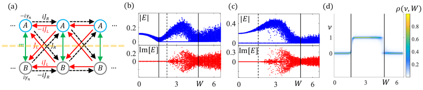
Figure A1: (a) Lattice representation of the Hamiltonian in Eq. A1, with on-site loss (gain) rate $\gamma_{n}$ for $A$ ($B$) sites. The tunneling gain (loss) $\kappa_{n}$ is encoded in $J_{L}=\frac{J-\kappa_{n}}{2}$ and $J_{R}=\frac{J+\kappa_{n}}{2}$. (b,c) The band structures around $E=0$ as a function of disorder strength for $m=1.1$ and $m=0.8$ respectively, with $W=W_{\gamma}=8W_{\kappa}$, $\kappa_{\text{b}}=0.1$. The scattered points show the first 20 energy levels around $E=0$ with 10 disorder configurations. The gap between the bulk and zero-energy edge states around $W=3$ is due to the low density of states, which will be filled if more disorder configurations are considered. (d) The winding number distribution $\rho(\nu,W)$ of 1000 disorder configurations. $\rho(\nu,W)=\frac{1}{D}\sum_{d=1}^{D}\frac{\varepsilon^{2}}{[\nu-\nu_{d}(W)]^{2}+\varepsilon^{2}}$, $\nu_{d}(W)$ is the winding number of the $d$-th disorder configuration with disorder strength $W$, $D=1000$ is the total number of disorder configurations, and each $\nu_{d}(W)$ is replaced by a narrow Lorentz function with width $\varepsilon=0.02$. In (b-d), the solid and dashed vertical lines are the phase boundary and PT-symmetry breaking point, respectively.

VI Appendix B: Experimental realization

In the main text, we have considered the realization of our model using coupled micro-ring cavities. As we discussed in the main text, the non-Hermiticity is induced by gain and loss in the coupler cavities. Here we give more details. Let us consider the coupling between two site cavities. In the presence of gain and loss in the coupler cavity, the tight-binding Hamiltonian for the clockwise modes can be written as Sci.Rep.5.13376

$$H_{\text{cw}}=re^{g}c_{B}^{{\dagger}}c_{A}+re^{-g}c_{A}^{{\dagger}}c_{B},$$ (A2)

where $r$ is determined by the coupling strength between the site and coupler cavities, and $g$ is determined by the gain and loss strength, leading to $m=r\cosh(g)$ and $\gamma_{n}=r\sinh(g)$. While for the counterclockwise modes, the Hamiltonian reads

$$H_{\text{ccw}}=re^{-g}c_{B}^{{\dagger}}c_{A}+re^{g}c_{A}^{{\dagger}}c_{B}=H_{\text{cw}}^{\dagger}.$$ (A3)

Therefore, we obtain the total Hamiltonian of Eq. 5 in the main text, with the clockwise and counterclockwise modes playing the role of pseudospin degrees of freedom.

In the single coupler case, the system always stays in the PT-symmetric region with $|\gamma_{n}|<m$. Though this does not prevent us from observing the non-Hermitian TAIs, the system has some other shortcomings. Once the photonic circuit is fabricated, the tunability of $m$ and $\gamma_{n}$ is very limited. Even though gain and loss can be controlled simply by varying the pumping strength, $m$ and $\gamma_{n}$ cannot be tuned independently. A different disorder configuration may require additional sample fabrication. Fortunately, all these shortcomings can be overcome by introducing a second coupler cavity, as shown in Fig. A2(b). By controlling the interference between two couplers Yariv.Photonics ; hafezi2011robust ; PhysRevLett.118.083603 ; PhysRevA.97.043841 , the Hermitian and non-Hermitian parts of the tunnelling become $m=r[\cosh(g_{1})-\cosh(g_{2})]$ and $\gamma_{n}=r[\sinh(g_{1})-\sinh(g_{2})]$, which can be tuned independently to arbitrary region (PT-symmetric or PT-breaking regions) by simply gain and loss control. This allows the study of various non-Hermitian disorder configurations using one sample.

Now we show how the input-output Sagnac waveguide allows the measurement in the spin basis $|\pm\rangle$. As shown in Fig. A2(a), the input-output waveguide is a ring interferometer with a $50:50$ beam splitter (BS). Let us denote the input-output field operators as $c_{1,\text{in}}$, $c_{1,\text{in}}$ and $c_{1,\text{out}}$ $c_{1,\text{out}}$, their relations with the field operators $c_{\uparrow}^{\prime}$ and $c_{\downarrow}^{\prime}$ inside the Sagnac interferometer are Yariv.Photonics ; hafezi2011robust

$$\left[\begin{array}[]{c}c_{\uparrow,\text{in}}^{\prime}\\ c_{\downarrow,\text{in}}^{\prime}\end{array}\right]=\left[\begin{array}[]{cc}\frac{1}{\sqrt{2}}&-\frac{1}{\sqrt{2}}\\ \frac{1}{\sqrt{2}}&\frac{1}{\sqrt{2}}\end{array}\right]\left[\begin{array}[]{c}c_{1,\text{in}}\\ c_{2,\text{in}}\end{array}\right],\text{ and }\left[\begin{array}[]{c}c_{1,\text{out}}\\ c_{2,\text{out}}\end{array}\right]=\left[\begin{array}[]{cc}\frac{1}{\sqrt{2}}&\frac{1}{\sqrt{2}}\\ \frac{1}{\sqrt{2}}&-\frac{1}{\sqrt{2}}\end{array}\right]\left[\begin{array}[]{c}c_{\uparrow,\text{out}}^{\prime}\\ c_{\downarrow,\text{out}}^{\prime}\end{array}\right].$$ (A16)

The Sagnac interferometer is weakly coupled with the cavity, thus we have

$$\left[\begin{array}[]{c}c_{\uparrow,\text{out}}^{\prime}\\ c_{\downarrow,\text{out}}^{\prime}\end{array}\right]=\left[\begin{array}[]{c}e^{i\varphi}\sqrt{1-\epsilon^{2}}c_{\uparrow,\text{in}}^{\prime}+\epsilon c_{\uparrow}\\ e^{i\varphi}\sqrt{1-\epsilon^{2}}c_{\downarrow,\text{in}}^{\prime}+\epsilon c_{\downarrow}\end{array}\right],$$ (A21)

where $\epsilon$ is the coupling rate and $\varphi$ is the phase delay of the Sagnac interferometer. We choose the gauge such that the phase for $c_{\uparrow}$ and $c_{\downarrow}$ in the above equation is zero. According to Eqs. A16 and A21, we obtain

$$\left[\begin{array}[]{c}c_{1,\text{out}}\\ c_{2,\text{out}}\end{array}\right]=\left[\begin{array}[]{c}e^{i\varphi}\sqrt{1-\epsilon^{2}}c_{1,\text{in}}+\epsilon c_{+}\\ e^{i\varphi}\sqrt{1-\epsilon^{2}}c_{2,\text{in}}+\epsilon c_{-}\end{array}\right],$$ (A26)

with $c_{\pm}=\frac{c_{\uparrow}\pm c_{\downarrow}}{\sqrt{2}}$. We see that the input-output port 1 and port 2 are coupled with the spin states $|\pm\rangle$ respectively, which allow us to excite and measure the photons in the $\tau^{x}$ basis. To measure the biorthogonal chiral displacement, we first prepare the initial state $|\phi_{0}\rangle$ by exciting the $|+\rangle$ state at A site of unit cell $n=0$ with a narrow pulse, then let the system evolve to $|\phi_{t}\rangle$ at time $t$. The output field intensities of the two ports at time $t$ are proportional to the photon field intensities in state $|\pm\rangle$, respectively. We can measure the output field intensities at each site and obtain $I_{1}(n,\alpha)$ for port 1, and $I_{2}(n,\alpha)$ for port 2, with $\alpha=0,1$ corresponding to $A,B$ sublattice sites respectively. Then, Eq. 6 in the main text can be written as: $\mathcal{C}(t)=\frac{2}{I_{\text{tot}}}\sum_{n}n[I_{1}(n,0)+I_{2}(n,1)-I_{2}(n,0)-I_{1}(n,1)]$, with total intensity $I_{\text{tot}}=\sum_{n}I_{1}(n,0)+I_{2}(n,0)+I_{1}(n,1)+I_{2}(n,1)$.

In realistic experiments, fabrication of large arrays of coupled micro-ring cavities is a mature technology and using auxiliary coupling waveguides with gain/loss arms to generate asymmetric tunneling has been demonstrated in a very recent experiment science.aba8996 . Moreover, the clean non-Hermitian SSH Hamiltonian has also been realized in electronic circuits with site addressability arXiv1907.11562 , where disorders can be introduced simply. With two SSH electronic circuits, we can probe the bulk topology (based on the Ramsey interferometer scheme) by measuring the interference between local resonators from the two circuits (i.e., in the $\tau^{x}$ basis), and this can be done since both amplitude and phase of the local resonators can be measured. Therefore, the experimental realization and detection of our non-Hermitian topological Anderson states should not represent a major difficulty.

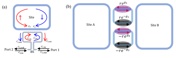
Figure A2: (a) Input-output waveguide for measuring photon distributions in the spin basis $|\pm\rangle$. (b) Site cavities coupled by two coupler cavities which allow the full tunability of the tunnelings through gain and loss control.

VII Appendix C: The winding number

As we defined in the main text, the winding number is

$$\nu = \frac{1}{4}\mathcal{T}\{Q\Gamma[\hat{X},Q]+Q^{\dagger}\Gamma[\hat{X},Q^{\dagger}]\}=\frac{1}{4}\mathcal{T}\{Q\Gamma[\hat{X},Q]\}+h.c.,$$ (A27)

where the first term $\mathcal{T}\{Q\Gamma[\hat{X},Q]\}$ corresponds to directly applying the Hermitian formula to the flattened non-Hermitian Hamiltonian $Q$, this term is not guaranteed to be real for a general non-Hermitian system since $Q\neq Q^{\dagger}$. In our model, we find that $\mathcal{T}\{Q\Gamma[\hat{X},Q]\}$ may have a small imaginary part in the PT-symmetry breaking region for each disorder configuration, and for parameters away from the phase transition points, its disorder average can be nearly real with imaginary part $\ll 1$.

We have considered the open boundary conditions in this paper, and a naive evaluation of the trace in calculating $\nu$ yields identical zero, since the contribution from the bulk states is canceled exactly by the boundary modes (we will discuss this in detail at the end of this section). Here we follow the idea in Ref. PhysRevLett.113.046802 ; PhysRevB.89.224203 ; science.aat3406 , and evaluate the trace per volume in Eq. A27 over the central part of the lattice chain (Here we exclude 100 lattice sites from each ends of the chain). Nevertheless, we find that, beside the strong fluctuations at the phase boundaries, the winding number also fluctuates more strongly in the PT-symmetry breaking region than the PT-symmetric region. The reasons are discussed in the following.

For a clean system, it is known that the PT-symmetry breaking is accompanied by the appearance of exceptional points where more than one right (left) eigenstates can coalesce and the Hamiltonian is defective. For the disorder driven PT-symmetry breaking studied here, it is also possible that the Hamiltonian becomes defective for certain specific disorder configurations (with fixed disorder strength). A defective Hamiltonian can not be flattened in the form of Eq. (1) in the main text. Fortunately, if we consider a finite lattice with finite disorder configurations, the probability for the random Hamiltonian to be defective is zero, as confirmed by our numerical simulations. On the other hand, in the thermodynamic limit (where the system is infinite), we can always get the specific disorder configuration at certain spatial interval such that the Hamiltonian is defective. In this case, we have infinite number of eigenstates (localized) and the probability for a state to coalesce with others is zero. As a result, we can safely exclude these defective disorder configurations in the calculation of the winding number as long as their occurrence probability is zero, which shares the same spirit as that one can exclude the exceptional points from the integral over the Brillouin zone when calculating the clean-system winding number PhysRevLett.121.213902 . In actual practice, we do not need to exclude any disorder configurations in the numerical simulations, as we adopt a finite lattice and consider finite number of disorder configurations, where the Hamiltonian is found to be always non-defective.

Though the Hamiltonian is always non-defective in the numerical simulations, we do find that there are more chances to obtain two nearly coalescing states (where the Hamiltonian is close to be defective) in the gapless PT-symmetry breaking region than other regions. Let us denote such two nearly identical states as $|\Psi_{1}^{R}\rangle$, $|\Psi_{2}^{R}\rangle$ and the corresponding left eigenstates as $|\Psi_{1}^{L}\rangle$, $|\Psi_{2}^{L}\rangle$, with energy given by $E_{d}$. The biorthonormality requires that $\langle\Psi_{1}^{L}|\Psi_{2}^{R}\rangle=0$ but $\langle\Psi_{1}^{L}|\Psi_{1}^{R}\rangle=1$. Recall that $|\Psi_{1}^{R}\rangle$ and $|\Psi_{2}^{R}\rangle$ are nearly identical, therefore, the distributions $P_{1}(n,\alpha)=\langle\Psi_{1}^{L}(n,\alpha)|\Psi_{1}^{R}(n,\alpha)\rangle$ must have amplitudes $|P_{1}(n,\alpha)|$ much larger than $1$ for some sites (the chiral symmetry $\sum_{n}P_{1}(n,0)=\sum_{n}P_{1}(n,1)=0.5$ is still satisfied). Similar analysis applies to state $|\Psi_{2}^{R}\rangle$. These properties of $|\Psi_{1,2}^{R}\rangle$ would lead to stronger fluctuations in the calculated winding number, especially when i) $P_{1}(n,\alpha)$ is occasionally distributed around the boundary of the central trace volume, or ii) $E_{d}\simeq 0$ since $|P_{1}(n,0)|$ would be much larger or smaller than $|P_{1}(n,1)|$, which is also the reason why the fluctuation becomes more significant after the band gap closing at $E=0$, or iii) the system size is too small. Though the fluctuations of the calculated winding numbers are stronger than the Hermitian models, clear phase boundaries can still be obtained, as shown in Fig. 2 in the main text. The calculated winding number is mainly distributed near the averaged value $\nu=1$ ($\nu=0$) in the topological (trivial) phase, as further confirmed in Fig. A1(d) where more disorder configurations ($\sim 1000$) are considered.

The existence of zero edge modes can be determined analytically using $\Lambda_{\alpha}$. While for the winding number $\nu$, it is hard to obtain an analytic formula as a function of system parameters (even for Hermitian disorders). To connect the existence of zero edge modes and non-trivial real-space winding, we define the biorthogonal chiral displacement of the two zero edge modes (one on each boundary), which reads

$$\mathcal{C}_{\text{edge}}=\frac{1}{4N}\sum_{\alpha}\langle\Psi_{0,\alpha}^{L}|\Gamma\hat{X}|\Psi_{0,\alpha}^{R}\rangle+h.c.$$ (A28)

with $\alpha=0,1$ the sublattice index and $2N$ the total number of unit cells. $|\Psi_{0,\alpha}^{L,R}\rangle$ corresponds to the zero edge mode occupying sublattice site $\alpha$, thus it is located at the boundary end with sublattice site $\alpha$. If there exist two zero edge modes, we have $\sum_{\alpha}\langle\Psi_{0,\alpha}^{L}|\Gamma\hat{X}|\Psi_{0,\alpha}^{R}\rangle=\langle\Psi_{0,0}^{L}|\hat{X}|\Psi_{0,0}^{R}\rangle-\langle\Psi_{0,1}^{L}|\hat{X}|\Psi_{0,1}^{R}\rangle\simeq-2N$, and thereby $\mathcal{C}_{\text{edge}}=-1$. If there is no zero edge mode, we simply have $\mathcal{C}_{\text{edge}}=0$.

On the other hand, the real-space winding number $\nu$ is encoded in the localized bulk states. Suppose we can separate the bulk states from the zero edge modes, so we can use the bulk states (i.e., the flattened Hamiltonian $Q$ only contains the bulk states) to calculate the real-space winding number defined in Eq. A27 with the trace per volume evaluated over the whole lattice chain. Then the winding number equals to the bulk biorthogonal chiral displacement,

$$\nu = \frac{1}{4}\mathcal{T}\{Q\Gamma[\hat{X},Q]\}+h.c.=\frac{1}{2}\mathcal{T}\{Q\Gamma\hat{X}Q\}+h.c.$$ (A29)

$$= \frac{1}{4N}\sum_{j,s}\langle\Psi_{j,s}^{L}|\Gamma\hat{X}|\Psi_{j,s}^{R}\rangle+h.c.,$$

where $j,s$ run over the bulk states in the summation, and we have used $Q\Gamma=-\Gamma Q$ in the derivation. We find that $\mathcal{C}_{\text{edge}}+\nu=0$ if the Hamiltonian is non-defective because $\mathcal{C}_{\text{edge}}+\nu=\frac{1}{2}\mathcal{T}\{\mathbb{I}\Gamma\hat{X}\}+h.c.$ and $\mathbb{I}=\sum_{j,s}|\Psi_{j,s}^{R}\rangle\langle\Psi_{j,s}^{L}|+\sum_{\alpha}|\Psi_{0,\alpha}^{R}\rangle\langle\Psi_{0,\alpha}^{L}|$ satisfies $\mathbb{I}|\phi\rangle=|\phi\rangle$ for arbitrary $|\phi\rangle$ if the Hamiltonian is non-defective. Fortunately, if we consider a finite lattice with finite disorder configurations, the probability for the random Hamiltonian to be defective is zero, as confirmed by our numerical simulations. Therefore, the existence of zero edge modes (i.e., $\mathcal{C}_{\text{edge}}=-1$) is connected to non-trivial real-space winding number $\nu=1$ encoded in the bulk states. We have numerically verified $\mathcal{C}_{\text{edge}}$ and bulk $\nu$ in the gapped region where the bulk states can be separated from zero edge modes.

We want to point out that, the non-Hermitian topology is encoded in the bulk states under open boundary condition supporting zero edge states. Numerically, it is hard to separate the zero edge states from bulk states in the strong disorder region with gapless bulk spectrum. Instead, we keep all the states and directly evaluate the trace per volume in Eq. A27 over the central part of the system to eliminate the effects of zero edge modes.

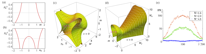
Figure A3: (a) (b) Zero-energy-mode biorthogonal localization length as functions of $m$ (with $\kappa_{\text{b}}=0.1$) and $\kappa_{\text{b}}$ (with $m=1.1$). $W=W_{\gamma}=8W_{\kappa}=2$. (c) (d) The delocalized critical surfaces on the parameter space ($m$, $\gamma_{\text{b}}$, $W$) and ($m$, $W_{\kappa}$, $W_{\gamma}$) with $W=W_{\gamma}=8W_{\kappa}$. (e) The IPR of all bulk eigenstates at different disorder strengths $W=W_{\gamma}=8W_{\kappa}$. $j$ is the eigenvalue index and the system contains 200 lattice sites ($N=50$). Other parameters are the same as Fig. 3c in the main text.

VIII Appendix D: Biorthogonal localization length

Different from Hermitian systems, here the eigenstates (both left and right ones) cannot be interpreted as the probability amplitude of particle’s distribution. In certain parameter regions (including certain phase transition points), we may even have all left/right eigenstates localized at the boundary due to non-Hermitian skin effects. It is a priori unclear how to characterize the localization-delocalization criticality for the non-Hermitian disorder systems. Given the fact that the left and right eigenstates are inequivalent, we need to take into account both of them to characterize the localization. For the zero-energy modes, the eigenequations $H|\Psi_{0}^{R}\rangle=0$ and $H^{{\dagger}}|\Psi_{0}^{L}\rangle=0$ are

$$0 = (J-\kappa_{n})|\Psi_{0}^{R}(n+1,0)\rangle+(m+\gamma_{n})|\Psi_{0}^{R}(n,0)\rangle$$

$$0 = (m-\gamma_{n+1})|\Psi_{0}^{R}(n+1,1)\rangle+(J+\kappa_{n})|\Psi_{0}^{R}(n,1)\rangle$$

$$0 = (J+\kappa_{n})|\Psi_{0}^{L}(n+1,0)\rangle+(m-\gamma_{n})|\Psi_{0}^{L}(n,0)\rangle$$

$$0 = (m+\gamma_{n+1})|\Psi_{0}^{L}(n+1,1)\rangle+(J-\kappa_{n})|\Psi_{0}^{L}(n,1)\rangle.$$ (A30)

The solutions are

$$|\Psi_{0}^{R}(n+1,\alpha)\rangle = -\left[\frac{m+(-1)^{\alpha}\gamma_{n+\alpha}}{J-(-1)^{\alpha}\kappa_{n}}\right]^{\eta_{\alpha}}|\Psi_{0}^{R}(n,\alpha)\rangle$$

$$|\Psi_{0}^{L}(n+1,\alpha)\rangle = -\left[\frac{m-(-1)^{\alpha}\gamma_{n+\alpha}}{J+(-1)^{\alpha}\kappa_{n}}\right]^{\eta_{\alpha}}|\Psi_{0}^{L}(n,\alpha)\rangle,$$ (A31)

with $\alpha=0,1$ and $\eta_{\alpha}=\pm 1$ corresponding to sublattice sites $A$ and $B$, respectively. We obtain the biorthogonal distributions $P(n,\alpha)=\langle\Psi_{0}^{L}(n,\alpha)|\Psi_{0}^{R}(n,\alpha)\rangle$ as given in the main text (by setting $J=1$ as the energy unit),

$$P(n,\alpha)=P(0,\alpha)\prod_{n^{\prime}=0}^{n-1}\left(\frac{m-\gamma_{n^{\prime}+\alpha}^{2}}{1-\kappa_{n^{\prime}}^{2}}\right)^{\eta_{\alpha}}.$$ (A32)

The zero-energy-mode biorthogonal localization lengths are

$$\Lambda_{\alpha}^{-1} = -\frac{1}{2}\lim_{n\rightarrow\infty}\frac{1}{n}\ln\left|\frac{P(n,\alpha)}{P(0,\alpha)}\right|$$ (A33)

$$= \lim_{n\rightarrow\infty}\frac{\eta_{\alpha}}{2n}\sum_{n^{\prime}=0}^{n-1}\left(\ln|1-\kappa_{n^{\prime}}^{2}|-\ln|m-\gamma_{n^{\prime}+\alpha}^{2}|\right).$$

According to Birkhoff’s ergodic theorem, we can use the ensemble average to evaluate $\Lambda_{\alpha}$

$$\Lambda_{0}^{-1}=-\Lambda_{1}^{-1} = \frac{1}{2}\int_{\gamma_{\text{b}}-W_{\gamma}/2}^{\gamma_{\text{b}}+W_{\gamma}/2}d\gamma\int_{\kappa_{\text{b}}-W_{\kappa}/2}^{\kappa_{\text{b}}+W_{\kappa}/2}d\kappa\left(\ln|1-\kappa^{2}|-\ln|m-\gamma^{2}|\right)$$ (A34)

$$= \sum_{s,s^{\prime}=\pm}\left[\ln\frac{|W_{\kappa}+2s+2ss^{\prime}\kappa_{\text{b}}|^{\frac{s+ss^{\prime}\kappa_{\text{b}}}{2W_{\kappa}}}|(W_{\kappa}+2s\kappa_{\text{b}})^{2}-4|^{1/8}}{|W_{\gamma}+2ms+2ss^{\prime}\gamma_{\text{b}}|^{\frac{ms+ss^{\prime}\gamma_{\text{b}}}{2W_{\gamma}}}|(W_{\gamma}+2s\gamma_{\text{b}})^{2}-4m^{2}|^{1/8}}\right].$$

Follow a similar analysis as in Ref. PhysRevLett.113.046802 ; PhysRevB.89.224203 ; science.aat3406 , we find that, except for some special cases $|W_{\kappa}\pm 2\kappa_{\text{b}}|=2$ and $|W_{\gamma}\pm 2\gamma_{\text{b}}|=2|m|$, $\Lambda_{\alpha}^{-1}$ is analytic at the critical phase boundary $\kappa_{\text{b}}^{c}$ and $m^{c}$ with expansion $\Lambda_{0}^{-1}(m,\kappa_{\text{b}})=a_{m}(m-m^{c})+a_{\kappa}(\kappa_{\text{b}}-\kappa_{\text{b}}^{c})+\cdots$ [as shown in Figs. A3(a) and A3(b)], leading to the critical exponent $1$. For the special critical cases, one has $\Lambda_{0}^{-1}(m)\sim(m-m^{c})\ln|m-m^{c}|$ with fixed $\kappa_{\text{b}}$, or $\Lambda_{0}^{-1}(\kappa_{\text{b}})\sim(\kappa_{\text{b}}-\kappa_{\text{b}}^{c})\ln|\kappa_{\text{b}}-\kappa_{\text{b}}^{c}|$ with fixed $m$.

In Figs. A3(c) and A3(d), we also plot the phase diagrams in the parameter space ($m$, $\gamma_{\text{b}}$, $W$) and ($m$, $W_{\kappa}$, $W_{\gamma}$) obtained from $\Lambda_{0}$. Here $W=W_{\gamma}=8W_{\kappa}$. We see that the system is topological (trivial) in the $W_{\kappa}\rightarrow\infty$ ($W_{\gamma}\rightarrow\infty$). Due to the competition between Hermitian ($m$) and non-Hermitian ($\gamma_{\text{b}}$) tunnelings which tend to weaken each other, the system stays in the topological phase up to very large $m$ and $\gamma_{\text{b}}$ along the directions $|m|=|\gamma_{\text{b}}|$.

When $E\neq 0$, it is difficult to obtain the analytic expression of the localization length. Here we numerically calculate the biorthogonal localization lengths using the transfer matrix method RevModPhys.80.1355 , where the transfer matrix for right (left) eigenstates can be obtained using $H$ ($H^{{\dagger}}$). The eigenequations $H|\Psi_{E}^{R}\rangle=E|\Psi_{E}^{R}\rangle$ and $H^{{\dagger}}|\Psi_{E}^{L}\rangle=E^{\ast}|\Psi_{E}^{L}\rangle$ can be written as

$$\left[\begin{array}[]{c}\Psi_{E}^{R}(\widetilde{n},0)\\ \Psi_{E}^{R}(\widetilde{n},1)\end{array}\right]=M_{\widetilde{n}}^{R}\left[\begin{array}[]{c}\Psi_{E}^{R}(0,0)\\ \Psi_{E}^{R}(0,1)\end{array}\right],\text{ with }M_{\widetilde{n}}^{R}=\prod_{n=0}^{\widetilde{n}-1}\left[\begin{array}[]{cc}-\frac{m+\gamma_{n}}{1-\kappa_{n}}&\frac{E}{1-\kappa_{n}}\\ -\frac{E(m+\gamma_{n})}{(1-\kappa_{n})(m-\gamma_{n+1})}&\frac{E^{2}-1+\kappa_{n}^{2}}{(1-\kappa_{n})(m-\gamma_{n+1})}\end{array}\right]$$

and similarly for $|\Psi_{E}^{L}\rangle$ with

$$M_{\widetilde{n}}^{L}=\prod_{n=0}^{\widetilde{n}-1}\left[\begin{array}[]{cc}-\frac{m-\gamma_{n}}{1+\kappa_{n}}&\frac{E^{\ast}}{1+\kappa_{n}}\\ -\frac{E^{\ast}(m-\gamma_{n})}{(1+\kappa_{n})(m+\gamma_{n+1})}&\frac{E^{\ast 2}-1+\kappa_{n}^{2}}{(1+\kappa_{n})(m+\gamma_{n+1})}\end{array}\right].$$

The biorthogonal localization length is defined as

$$\Lambda_{E}^{-1}=\lim_{\widetilde{n}\rightarrow\infty}\frac{\ln|\lambda_{\widetilde{n}}^{R}\lambda_{\widetilde{n}}^{L}|}{2\widetilde{n}},$$ (A35)

with $\lambda_{\widetilde{n}}^{R}$ ($\lambda_{\widetilde{n}}^{L}$) the larger eigenvalue of $M_{\widetilde{n}}^{R}$ ($M_{\widetilde{n}}^{L}$) Z.Phys.B.53 ; PhysRevB.29.3111 . Our numerical results are shown in Fig. 3(c) in the main text, which indicate that all states with $E\neq 0$ are localized in every instance with disorders. At $E=0$, $\Lambda_{E}^{-1}$ is consistent with the analytic zero-energy-mode biorthogonal localization length.

The localization properties can also be characterized by the inverse participation ratio (IPR) of the eigenstates, and larger IPR corresponds to stronger localization RevModPhys.80.1355 . Here we define the biorthogonal IPR as

$$\text{IPR}_{\widetilde{j}}=\frac{\sum_{n,\alpha}|\langle\Psi^{L}_{\widetilde{j}}(n,\alpha)|\Psi^{R}_{\widetilde{j}}(n,\alpha)\rangle|^{4}}{\sum_{n,\alpha}|\langle\Psi^{L}_{\widetilde{j}}(n,\alpha)|\Psi^{R}_{\widetilde{j}}(n,\alpha)\rangle|^{2}},$$ (A36)

with $\widetilde{j}=(j,\pm)$ the eigenvalue index. The averaged IPR is defined as $\text{IPR}=\frac{1}{L}\sum_{\widetilde{j}}\text{IPR}_{\widetilde{j}}$ with $L$ the total number of sites. In Fig. A3(e), we plot the IPR${}_{\widetilde{j}}$ near the phase boundaries for all bulk states with $E\neq 0$, which are well above $1/L$, indicating strong localization.

IX Appendix E: Biorthogonal chiral displacement

In this section, we prove that the averaged Biorthogonal chiral displacement converges to the winding number in the PT-symmetric region. In the presence of disorder, the trace over the whole system may be replaced by a disorder average over a single unit cell according to Birkhoff’s ergodic theorem PhysRevLett.113.046802 ; PhysRevB.89.224203 ; science.aat3406 . We can evaluate the winding number at unit cell $n=0$, which is

$$\nu(0) = \frac{1}{4}\sum_{\alpha=A,B}\langle 0_{\alpha}|Q\Gamma[\hat{X},Q]|0_{\alpha}\rangle+h.c.$$ (A37)

$$= \frac{1}{4}\sum_{\alpha}\langle 0_{\alpha}|Q\Gamma\hat{X}Q|0_{\alpha}\rangle+h.c.$$

$$= \frac{1}{4}\sum_{\alpha}\langle 0_{\alpha}|(\mathbb{I}-2P_{-})\Gamma\hat{X}(\mathbb{I}-2P_{-})|0_{\alpha}\rangle+h.c.,$$

with $\mathbb{I}=P_{+}+P_{-}$. In the PT-symmetric region (without eigenstates coalescing), the eigenstates form a complete biorthonormal basis, and an arbitrary state $|\phi\rangle$ can be expanded as $|\phi\rangle=\sum_{s=\pm,j}\phi_{j,s}|\Psi_{j,s}^{R}\rangle$ with $\phi_{j,s}=\langle\Psi_{j,s}^{L}|\phi\rangle$, and $\mathbb{I}|\phi\rangle=|\phi\rangle$. Therefore, we have

$$\nu(0) = \sum_{\alpha}\langle 0_{\alpha}|P_{-}\Gamma\hat{X}P_{-}|0_{\alpha}\rangle+h.c.$$ (A38)

$$= \sum_{\alpha}\left[\frac{1}{2}\sum_{s=\pm,j}a_{j,s}^{R}(\alpha)a_{j,s}^{L}(\alpha)\langle\Psi_{j,s}^{L}|\Gamma\hat{X}|\Psi_{j,s}^{R}\rangle+\sum_{j\neq j^{\prime}}a_{j,-}^{R}(\alpha)a_{j^{\prime},-}^{L}(\alpha)\langle\Psi_{j,-}^{L}|\Gamma\hat{X}|\Psi_{j^{\prime},-}^{R}\rangle\right]+h.c.,$$

with $a_{j,s}^{R}(\alpha)=\langle 0_{\alpha}|\Psi_{j,s}^{R}\rangle$ and $a_{j,s}^{L}(\alpha)=\langle\Psi_{j,s}^{L}|0_{\alpha}\rangle$. Similar to the Hermitian system, we find (numerically) that the off-diagonal part (the sum over $j\neq j^{\prime}$) in the above equation provides very small contributions, and

$$\nu(0)\simeq\frac{1}{2}\sum_{\alpha,s=\pm,j}a_{j,s}^{R}(\alpha)a_{j,s}^{L}(\alpha)\langle\Psi_{j,s}^{L}|\Gamma\hat{X}|\Psi_{j,s}^{R}\rangle+h.c.$$

The biorthogonal chiral displacement is defined as

$$\mathcal{C}_{A}(t)=\langle L(t)|\Gamma\hat{X}|R(t)\rangle+h.c.=\langle 0_{A}|\exp(iHt)\Gamma\hat{X}\exp(-iHt)|0_{A}\rangle+h.c.$$

$$=\sum_{j,s}a^{R}_{j,s}(A)a^{L}_{j,s}(A)\langle\Psi_{j,s}^{L}|\Gamma\hat{X}|\Psi_{j,s}^{R}\rangle+\sum_{(j,s)\neq(j^{\prime},s^{\prime})}a^{R}_{j,s}(A)a^{L}_{j^{\prime},s^{\prime}}(A)e^{i(E_{j,s}-E_{j^{\prime},s^{\prime}})t}\langle\Psi_{j,s}^{L}|\Gamma\hat{X}|\Psi_{j^{\prime},s^{\prime}}^{R}\rangle+h.c.$$ (A39)

In the PT-symmetric region, all eigenvalues $E_{j,s}$ are real. Therefore, the second term of Eq. A39 rapidly oscillates, which converges to zero when averaged over sufficiently long time sequences. The first term of Eq. A39 is time independent and gives the mean chiral displacement

$$\bar{\mathcal{C}}_{A}(\infty) = \sum_{j,s}a^{R}_{j,s}(A)a^{L}_{j,s}(A)\langle\Psi_{j,s}^{L}|\Gamma\hat{X}|\Psi_{j,s}^{R}\rangle+h.c.$$ (A40)

Similarly, we can calculate the chiral displacement $\bar{\mathcal{C}}_{B}(\infty)$ for initial state $|0_{B}\rangle$ and $\nu(0)=\bar{\mathcal{C}}(\infty)\equiv\frac{1}{2}[\bar{\mathcal{C}}_{A}(\infty)+\bar{\mathcal{C}}_{B}(\infty)]$. For Hermitian systems, one has $\bar{\mathcal{C}}_{A}(\infty)=\bar{\mathcal{C}}_{B}(\infty)$ science.aat3406 , and we find it also holds here. We can just use the chiral displacement $\mathcal{C}_{A}(t)$ to probe the topology and drop the subscript $A$.

X Appendix F: Effects of interaction

Generally, interaction is irrelevant for the photonic systems since photons do not interact with each other. While for atomic system, strong interaction is possible. If the bulk states have a gap around $E=0$, we expect that the topology and zero edge modes are not affected by interactions that are small compared to the gap. For the disordered system, the gap might be an averaged result (i.e., the probability to find bulk states vanishes within the gap around). On the other hand, the topology may be inhibited by interaction if the interaction is too strong or if the gap at $E=0$ disappears (which is typical for the topological states in strong disorder region). Further numerical simulations are needed to ascertain the interacting physics. One possible way is to calculate the topological invariant based on the many-body ground state (as defined in the following). Numerically, the many-body ground state can be obtained by exact diagonalization method, which may not be practicable since a large system is required to suppress the boundary effects. It is also possible to generalize the density matrix renormalization group method to non-Hermitian systems. We believe that the interaction effects in such non-Hermitian topological Anderson insulators are more subtle than that in the ordinary topological insulators, which is a very interesting direction worth to be addressed in future works.

Now we give a possible generalization of the winding number. We note that the non-interacting winding number equals to the biorthogonal chiral displacement averaged over occupied bulk states (i.e., $\nu=\frac{1}{2N}\sum_{j}\langle\Psi_{j,-}^{L}|\Gamma\hat{X}|\Psi_{j,-}^{R}\rangle+h.c.$ due to $\langle\Psi_{j,+}^{L}|\Gamma\hat{X}|\Psi_{j,+}^{R}\rangle=\langle\Psi_{j,-}^{L}|\Gamma\hat{X}|\Psi_{j,-}^{R}\rangle$). Therefore, we could define a many-body winding number as

$$\nu_{\text{int}}=\frac{1}{2N}\langle G^{L}|\Gamma X|G^{R}\rangle+h.c.,$$ (A41)

with $|G^{L,R}\rangle$ the left/right many-body ground state. The ground state has lowest real energy for a given particle number (which is still a good quantum number). If the lowest real level contains two or more states, we choose the one with lowest imaginary energy among them. For non-interacting particles, bosons and fermions share the same single-particle spectrum, zero edge modes and topological invariant. While for interacting many-body ground state, we need discuss bosons and fermions separately. It can be shown that, for fermions, the above many-body invariant with $2N-1$ interacting particles can be reduced to the non-interacting invariant if the non-interacting bulk states have a gap at $E=0$ (this is because, if we have $E=0$ bulk states, the particles in $|G^{L,R}\rangle$ may occupy zero edge modes instead of the zero bulk states). For the disordered system, this generalization is consistent with non-interacting invariant if the probability to find zero bulk states vanishes for a finite size lattice and a finite number of disorder configurations. While for bosons, if the interaction is weak, $|G^{L,R}\rangle$ may corresponds to occupation of all particles on a few low single-particle levels, which should be trivial. Interesting bosonic many-body topological states may emerge under strong interactions, for example, the many-body invariant of simple hardcore bosons (which can be mapped to non-interacting fermions that preserves density) is reduced to non-interacting fermion invariant.

In the following, we show how to reduce the many-body invariant in the non-interaction limit. The Hamiltonian can be written as

$$H=\sum_{j,s}E_{j,s}\beta_{R,j,s}^{{\dagger}}\beta_{L,j,s},$$

where $\beta_{L,j,s}=\sum_{n,\alpha}\mathcal{L}_{j,s;n,\alpha}c_{n,\alpha}$ and $\beta_{R,j,s}^{{\dagger}}=\sum_{n,\alpha}c_{n,\alpha}^{{\dagger}}\mathcal{R}_{n,\alpha;j,s}$, with $\mathcal{L}_{j,s;n,\alpha}=\langle\Psi_{j,s}^{L}|n,\alpha\rangle$ and $\mathcal{R}_{n,\alpha;j,s}=\langle n,\alpha|\Psi_{j,s}^{R}\rangle$. They satisfy $\beta_{L,j,s}\beta_{R,j^{\prime},s^{\prime}}^{{\dagger}}\pm\beta_{R,j^{\prime},s^{\prime}}^{{\dagger}}\beta_{L,j,s}=\delta_{j,j^{\prime}}\delta_{s,s^{\prime}}$, with $\pm$ corresponding to fermions and bosons, respectively.

Fermions: The non-interacting fermion ground state with $N_{p}$ (we assume $N_{p}\leq 2N$) particles is

$$|G^{R}\rangle=\prod_{j=1}^{N_{p}}\beta_{R,j,-}^{{\dagger}}|\text{vac}\rangle\text{ and }\langle G^{L}|=\langle\text{vac}|\prod_{j=1}^{N_{p}}\beta_{L,j,-}$$ (A42)

with ground state energy $\sum_{j}^{N_{p}}E_{j,-}$, here $|\text{vac}\rangle$ the vacuum state. If the Hamiltonian is non-defective, we have $\mathcal{R}_{n,\alpha;j,s}\beta_{L,j,s}=c_{n,\alpha}$ and $\beta_{R,j,s}^{{\dagger}}\mathcal{L}_{j,s;n,\alpha}=c_{n,\alpha}^{{\dagger}}$, thus the many-body invariant becomes

$$\nu_{\text{int}} = \frac{1}{2N}\langle G^{L}|\Gamma X|G^{R}\rangle+h.c.$$ (A43)

$$= \frac{1}{2N}\langle G^{L}|\sum_{n,\alpha}n(-1)^{\alpha}c_{n,\alpha}^{{\dagger}}c_{n,\alpha}|G^{R}\rangle+h.c.$$

$$= \frac{1}{2N}\sum_{n,\alpha,j,j^{\prime},s,s^{\prime}}n(-1)^{\alpha}\mathcal{L}_{j,s;n,\alpha}\mathcal{R}_{n,\alpha;j^{\prime},s^{\prime}}\langle G^{L}|\beta_{R,j,s}^{{\dagger}}\beta_{L,j^{\prime},s^{\prime}}|G^{R}\rangle+h.c.$$

$$= \frac{1}{2N}\sum_{j}^{N_{p}}\sum_{n,\alpha}n(-1)^{\alpha}\mathcal{L}_{j,-;n,\alpha}\mathcal{R}_{n,\alpha;j,-}+h.c.$$

$$= \frac{1}{2N}\sum_{j}^{N_{p}}\langle\Psi_{j,-}^{L}|\Gamma\hat{X}|\Psi_{j,-}^{R}\rangle+h.c.$$

$$= \frac{1}{4N}\sum_{j}^{N_{p}}\sum_{s=\pm}\langle\Psi_{j,s}^{L}|\Gamma\hat{X}|\Psi_{j,s}^{R}\rangle+h.c.$$

We have used $\langle\Psi_{j,+}^{L}|\Gamma\hat{X}|\Psi_{j,+}^{R}\rangle=\langle\Psi_{j,-}^{L}|\Gamma\hat{X}|\Psi_{j,-}^{R}\rangle$. If $N_{p}=2N-1$ and there is no zero bulk states, then $\nu_{\text{int}}$ is just the biorthogonal chiral displacement averaged over all single-particle bulk states, and thus $\nu_{\text{int}}=\nu$.

Bosons:The non-interacting boson ground state with $N_{p}$ particles is

$$|G^{R}\rangle=\frac{1}{\sqrt{N_{p}!}}(\beta_{R,1,-}^{{\dagger}})^{N_{p}}|\text{vac}\rangle\text{ and }\langle G^{L}|=\langle\text{vac}|\frac{1}{\sqrt{N_{p}!}}(\beta_{L,1,-})^{N_{p}}$$ (A44)

and the many-body invariant becomes

$$\nu_{\text{int}}\ =\frac{N_{p}}{2N}\langle\Psi_{1,-}^{L}|\Gamma\hat{X}|\Psi_{1,-}^{R}\rangle+h.c.,$$ (A45)

which is not quantized in general.

Acknowledgement. This work is supported by AFOSR (FA9550-16-1-0387, FA9550-20-1-0220), NSF (PHY-1806227), ARO (W911NF-17-1-0128), UTD internal seed grant. X.L. also acknowledges support from the USTC start-up funding.

Data Availability. The data that support the plots within this paper and other findings of this paper are available from the corresponding author upon reasonable request

References

- (1) D. Xiao, M.-C. Chang, and Q. Niu, Berry phase effects on electronic properties, Rev. Mod. Phys. 82, 1959 (2010).
- (2) M. Hasan and C. Kane, Colloquium: topological insulators, Rev. Mod. Phys. 82, 3045 (2010).
- (3) X.-L. Qi and S.-C. Zhang, Topological insulators and superconductors, Rev. Mod. Phys. 83, 1057 (2011).
- (4) C.-K. Chiu, J. C. Y. Teo, A. P. Schnyder, and S. Ryu, Classification of topological quantum matter with symmetries, Rev. Mod. Phys. 88, 035005 (2016).
- (5) C. L. Kane and E. J. Mele, Topological Order and the Quantum Spin Hall Effect, Phys. Rev. lett. 95, 146802 (2005).
- (6) B. A. Bernevig, T. L. Hughes, S.-C. Zhang, Quantum Spin Hall Effect and Topological Phase Transition in HgTe Quantum Wells, Science 314, 1757 (2006).
- (7) M. König, S. Wiedmann, C. Brüne, A. Roth, H. Buhmann, L. W. Molenkamp, X.-L. Qi, S.-C. Zhang, Quantum Spin Hall Insulator State in HgTe Quantum Wells, Science 318, 766 (2007).
- (8) M. Aidelsburger, M. Atala, M. Lohse, J. T. Barreiro, B. Paredes, and I. Bloch, Realization of the Hofstadter Hamiltonian with Ultracold Atoms in Optical Lattices, Phys. Rev. lett. 111, 185301 (2013).
- (9) H. Miyake, G. A. Siviloglou, C. J. Kennedy, W. C. Burton, and W. Ketterle, Realizing the Harper Hamiltonian with Laser-Assisted Tunneling in Optical Lattices, Phys. Rev. lett. 111, 185302 (2013).
- (10) G. Jotzu, M. Messer, R. Desbuquois, M. Lebrat, T. Uehlinger, D. Greif, and T. Esslinger, Experimental realization of the topological Haldane model with ultracold fermions, Nature 515, 237 (2014).
- (11) N. Goldman, J. C. Budich, and P. Zoller, Topological quantum matter with ultracold gases in optical lattices, Nat. Phys. 12, 639 (2016).
- (12) N. R. Cooper, J. Dalibard, I. B. Spielman, Topological Bands for Ultracold Atoms, Rev. Mod. Phys. 91, 015005 (2019).
- (13) F. D. M. Haldane, and S. Raghu, Possible Realization of Directional Optical Waveguides in Photonic Crystals with Broken Time-Reversal Symmetry, Phys. Rev. Lett. 100, 013904 (2008).
- (14) M. Hafezi, E. A. Demler, M. D. Lukin, and J. M. Taylor, Robust optical delay lines with topological protection, Nature Phys. 7, 907 (2011).
- (15) K. Fang, Z. Yu, and S. Fan, Realizing effective magnetic field for photons by controlling the phase of dynamic modulation, Nature Photon. 6, 782 (2012).
- (16) L. Lu, J. D. Joannopoulos, and M. Soljačić, Topological photonics, Nature Photon. 8, 821 (2014).
- (17) Y. E. Kraus, Y. Lahini, Z. Ringel, M. Verbin, and O. Zilberberg, Topological states and adiabatic pumping in quasicrystals, Phys. Rev. Lett. 109, 106402 (2012).
- (18) M. Hafezi, S. Mittal, J. Fan, A. Migdall and J. M. Taylor, Imaging topological edge states in silicon photonics, Nature Photon. 7, 1001 (2013).
- (19) T. Ozawa, H. M. Price, A. Amo, N. Goldman, M. Hafezi, L. Lu, M. Rechtsman, D. Schuster, J. Simon, O. Zilberberg, and I. Carusotto, Topological Photonics, Rev. Mod. Phys. 91, 015006 (2019).
- (20) G. Ma, M. Xiao and C. T. Chan, Topological phases in acoustic and mechanical systems, Nat. Rev. Phys. 1, 281 (2019).
- (21) C. M. Bender, Making Sense of Non-Hermitian Hamiltonians, Rep. Prog. Phys. 70, 947 (2007).
- (22) V. M. Martinez Alvarez, J. E. Barrios Vargas, M. Berdakin, and L. E. F. Foa Torres, Topological states of non-Hermitian systems, Eur. Phys. J. Spec. Top. 227, 1295 (2018).
- (23) K. G. Makris, R. El-Ganainy, D. N. Christodoulides, and Z. H. Musslimani, Beam Dynamics in Symmetric Optical Lattices, Phys. Rev. Lett. 100, 103904 (2008).
- (24) A. Regensburger, C. Bersch, M.-A. Miri, G. Onishchukov, D. N. Christodoulides, and U. Peschel, Parity-time synthetic photonic lattices, Nature 488, 167 (2012).
- (25) S. Malzard, C. Poli, and H. Schomerus, Topologically Protected Defect States in Open Photonic Systems with Non-Hermitian Charge-Conjugation and Parity-Time Symmetry, Phys. Rev. Lett. 115, 200402 (2015).
- (26) Y. N. Joglekar, and A. K. Harter, Passive parity-time-symmetry-breaking transitions without exceptional points in dissipative photonic systems, Photon. Res. 6, A51 (2018).
- (27) H. Jing, S. K. Özdemir, X.-Y. Lü, J. Zhang, L. Yang, and F. Nori, -Symmetric Phonon Laser, Phys. Rev. Lett. 113, 053604 (2014).
- (28) B. Peng, Ş. K. Özdemir, S. Rotter, H. Yilmaz, M. Liertzer, F. Monifi, C. M. Bender, F. Nori, and L. Yang, Loss-induced suppression and revival of lasing, Science 346, 328 (2014).
- (29) J. M. Zeuner, M. C. Rechtsman, Y. Plotnik, Y. Lumer, S. Nolte, M. S. Rudner, M. Segev, and A. Szameit, Observation of a Topological Transition in the Bulk of a Non-Hermitian System, Phys. Rev. Lett. 115, 040402 (2015).
- (30) S. Weimann, M. Kremer, Y. Plotnik, Y. Lumer, S. Nolte, K. G. Makris, M. Segev, M. C. Rechtsman, and A. Szameit, Topologically protected bound states in photonic parity-time-symmetric crystals, Nat. Mater. 16, 433 (2017).
- (31) H. Zhao, P. Miao, M. H. Teimourpour, S. Malzard, R. El-Ganainy, H. Schomerus, and L. Feng, Topological hybrid silicon microlasers, Nat. Commun. 9, 981 (2018).
- (32) M. Parto, S. Wittek, H. Hodaei, G. Harari, M. A. Bandres, J. Ren, M. C. Rechtsman, M. Segev, D. N. Christodoulides, and M. Khajavikhan, Edge-Mode Lasing in 1D Topological Active Arrays, Phys. Rev. Lett. 120, 113901 (2018).
- (33) P. St-Jean, V. Goblot, E. Galopin, A. Lemaître, T. Ozawa, L. Le Gratiet, I. Sagnes, J. Bloch, and A. Amo, Lasing in topological edge states of a one-dimensional lattice, Nat. Photon. 11, 651 (2017).
- (34) M. A. Bandres, S. Wittek, G. Harari, M. Parto, J. Ren, M. Segev, D. N. Christodoulides, and M. Khajavikhan, Topological insulator laser: Experiments, Science 359, eaar4005 (2018).
- (35) M. Müller, S. Diehl, G. Pupillo, and P. Zoller, Engineered open systems and quantum simulations with atoms and ions, Adv. At. Mol. Opt. Phys. 61, 1 (2012).
- (36) Y. Ashida, S. Furukawa, and M. Ueda, Parity-time-symmetric quantum critical phenomena, Nat. Commun. 8, 15791 (2017).
- (37) H. Shen, and L. Fu, Quantum Oscillation from In-Gap States and a Non-Hermitian Landau Level Problem, Phys. Rev. Lett. 121, 026403 (2018).
- (38) M. Papaj, H. Isobe, and L. Fu, Nodal arc of disordered Dirac fermions and non-Hermitian band theory, Phys. Rev. B 99, 201107 (2019).
- (39) T. Yoshida, R. Peters, and N. Kawakami, Non-Hermitian perspective of the band structure in heavy-fermion systems, Phys. Rev. B 98, 035141 (2018).
- (40) Y. Xu, S.-T. Wang, and L.-M. Duan, Weyl Exceptional Rings in a Three-Dimensional Dissipative Cold Atomic Gas, Phys. Rev. Lett. 118, 045701 (2017).
- (41) J. Li, A. K. Harter, J. Liu, L. de Melo, Y. N. Joglekar, and L. Luo, Observation of parity-time symmetry breaking transitions in a dissipative Floquet system of ultracold atoms, Nat. Commun. 10, 855 (2019).
- (42) S. Lapp, J. Ang’ong’a, F. A. An, and B. Gadway, Engineering tunable local loss in a synthetic lattice of momentum states, New J. Phys. 21, 045006 (2019).
- (43) T. Helbig, T. Hofmann, S. Imhof, M. Abdelghany, T. Kiessling, L. W. Molenkamp, C. H. Lee, A. Szameit, M. Greiter, and R. Thomale, Generalized bulk-boundary correspondence in non-Hermitian topolectrical circuits, Nat. Phys. 16, 747 (2020).
- (44) K. Esaki, M. Sato, K. Hasebe, and M. Kohmoto, Edge states and topological phases in non-Hermitian systems, Phys. Rev. B 84, 205128 (2011).
- (45) A. K. Harter, T. E. Lee, and Y. N. Joglekar, -breaking threshold in spatially asymmetric Aubry-André and Harper models: Hidden symmetry and topological states, Phys. Rev. A 93, 062101 (2016).
- (46) T. E. Lee, Anomalous Edge State in a Non-Hermitian Lattice, Phys. Rev. Lett. 116, 133903 (2016).
- (47) S. Yao, F. Song, and Z. Wang, Non-Hermitian Chern Bands, Phys. Rev. Lett. 121, 136802 (2018).
- (48) S. Yao and Z. Wang, Edge States and Topological Invariants of Non-Hermitian Systems, Phys. Rev. Lett. 121, 086803 (2018).
- (49) F. K. Kunst, E. Edvardsson, J. C. Budich, and E. J. Bergholtz, Biorthogonal Bulk-Boundary Correspondence in Non-Hermitian Systems, Phys. Rev. Lett. 121, 026808 (2018).
- (50) K. Takata and M. Notomi, Photonic Topological Insulating Phase Induced Solely by Gain and Loss, Phys. Rev. Lett. 121, 213902 (2018).
- (51) Z. Gong, Y. Ashida, K. Kawabata, K. Takasan, S. Higashikawa, and M. Ueda, Topological Phases of Non-Hermitian Systems, Phys. Rev. X 8, 031079 (2018).
- (52) Y. Xiong, Why does bulk boundary correspondence fail in some non-hermitian topological models, J. Phys. Commun. 2, 035043 (2018).
- (53) S. Lieu, Topological phases in the non-Hermitian Su-Schrieffer-Heeger model, Phys. Rev. B 97, 045106 (2018).
- (54) D. Leykam, K. Y. Bliokh, C. Huang, Y. D. Chong, and F. Nori, Edge Modes, Degeneracies, and Topological Numbers in Non-Hermitian Systems, Phys. Rev. Lett. 118, 040401 (2017).
- (55) H. Shen, B. Zhen, and L. Fu, Topological Band Theory for Non-Hermitian Hamiltonians, Phys. Rev. Lett. 120, 146402 (2018).
- (56) H. Zhou, C. Peng, Y. Yoon, C. W. Hsu, K. A. Nelson, L. Fu, J. D. Joannopoulos, M. Soljačić, and B. Zhen, Observation of bulk Fermi arc and polarization half charge from paired exceptional points, Science 359, 1009 (2018).
- (57) A. Cerjan, S. Huang, K. P. Chen, Y. Chong, M. C. Rechtsman, Experimental realization of a Weyl exceptional ring, arXiv:1808.09541 (2018).
- (58) K. Kawabata, S. Higashikawa, Z. Gong, Y. Ashida, and M. Ueda, Topological unification of time-reversal and particle-hole symmetries in non-Hermitian physics, Nat. Commun. 10, 297 (2019).
- (59) A. Cerjan, M. Xiao, L. Yuan, and S. Fan, Effects of non-Hermitian perturbations on Weyl Hamiltonians with arbitrary topological charges, Phys. Rev. B 97, 075128 (2018).
- (60) L. Jin and Z. Song, Bulk-boundary correspondence in a non-Hermitian system in one dimension with chiral inversion symmetry, Phys. Rev. B 99, 081103 (2019).
- (61) C. H. Lee, G. Li, Y. Liu, T. Tai, R. Thomale, and X. Zhang, Tidal surface states as fingerprints of non-Hermitian nodal knot metals, arXiv:1812.02011 (2018).
- (62) C. H. Lee, and R. Thomale, Anatomy of skin modes and topology in non-Hermitian systems, Phys. Rev. B 99, 201103 (2019).
- (63) D. S. Borgnia, A. J. Kruchkov, and R.-J. Slager, Non-Hermitian Boundary Modes, arXiv:1902.07217 (2019).
- (64) L. Li, C. H. Lee, and J. Gong, Geometric characterization of non-Hermitian topological systems through the singularity ring in pseudospin vector space, Phys. Rev. B 100, 075403 (2019).
- (65) X. M. Yang, P. Wang, L. Jin, Z. Song, Visualizing Topology of Real-Energy Gapless Phase Arising from Exceptional Point, arXiv:1905.07109 (2019).
- (66) F. Song, S. Yao, and Z. Wang, Non-Hermitian Skin Effect and Chiral Damping in Open Quantum Systems, Phys. Rev. Lett. 123, 170401 (2019).
- (67) F. Song, S. Yao, and Z. Wang, Non-Hermitian Topological Invariants in Real Space, Phys. Rev. Lett. 123, 246801 (2019).
- (68) K. L. Zhang, H. C. Wu, L. Jin, and Z. Song, Topological phase transition independent of system non-Hermiticity, Phys. Rev. B 100, 045141 (2019).
- (69) X. Qiu, T.-S. Deng, Y. Hu, P. Xue, and W. Yi, Fixed Points and Dynamic Topological Phenomena in a Parity-Time-Symmetric Quantum Quench, iScience 20, 392 (2019).
- (70) K. Wang, X. Qiu, L. Xiao, X. Zhan, Z. Bian, B. C. Sanders, W. Yi, and P. Xue, Observation of emergent momentum-time skyrmions in parity-time-symmetric non-unitary quench dynamics, Nat. Commun. 10, 2293 (2019).
- (71) L. Xiao, T. Deng, K. Wang, G. Zhu, Z. Wang, W. Yi, and P. Xue, Observation of non-Hermitian bulk-boundary correspondence in quantum dynamics, arXiv:1907.12566 (2019).
- (72) L. Li, C. H. Lee, J. Gong, Topology-Induced Spontaneous Non-reciprocal Pumping in Cold-Atom Systems with Loss, arXiv:1910.03229 (2019).
- (73) X.-R. Wang, C.-X. Guo, S.-P. Kou, Defective Edge States and Anomalous Bulk-Boundary Correspondence in non-Hermitian Topological Systems, arXiv:1912.04024 (2019).
- (74) P. W. Anderson, Absence of Diffusion in Certain Random Lattices, Phys. Rev. 109, 1492, (1958).
- (75) D. S. Fisher, Random antiferromagnetic quantum spin chains, Phys. Rev. B 50, 3799, (1994).
- (76) M. Onoda, Y. Avishai, and N. Nagaosa, Localization in a Quantum Spin Hall System, Phys. Rev. Lett. 98, 076802, (2007).
- (77) D. N. Sheng, Z. Y. Weng, L. Sheng, and F. D. M. Haldane, Quantum Spin-Hall Effect and Topologically Invariant Chern Numbers, Phys. Rev. Lett. 97, 036808, (2006).
- (78) E. Prodan, T. L. Hughes, and B. A. Bernevig, Entanglement Spectrum of a Disordered Topological Chern Insulator, Phys. Rev. Lett. 105, 115501, (2010).
- (79) J. Li, R.-L. Chu, J. K. Jain, and S.-Q. Shen, Topological Anderson Insulator, Phys. Rev. Lett. 102, 136806, (2009).
- (80) H. Jiang, L. Wang, Q.-F. Sun, and X. C. Xie, Numerical study of the topological Anderson insulator in HgTe/CdTe quantum wells, Phys. Rev. B 80, 165316, (2009).
- (81) C. W. Groth, M. Wimmer, A. R. Akhmerov, J. Tworzydło, and C. W. J. Beenakker, Theory of the Topological Anderson Insulator, Phys. Rev. Lett. 103, 196805, (2009).
- (82) H.-M. Guo, G. Rosenberg, G. Refael, and M. Franz, Topological Anderson Insulator in Three Dimensions, Phys. Rev. Lett. 105, 216601, (2010).
- (83) A. Altland, D. Bagrets, L. Fritz, A. Kamenev, and H. Schmiedt, Quantum Criticality of Quasi-One-Dimensional Topological Anderson Insulators, Phys. Rev. Lett. 112, 206602, (2014).
- (84) P. Titum, N. H. Lindner, M. C. Rechtsman, and G. Refael, Disorder-Induced Floquet Topological Insulators, Phys. Rev. Lett. 114, 056801, (2015).
- (85) C. Liu, W. Gao, B. Yang, and S. Zhang, Disorder-Induced Topological State Transition in Photonic Metamaterials, Phys. Rev. Lett. 119, 183901, (2017).
- (86) I. Mondragon-Shem, T. L. Hughes, J. Song, and E. Prodan, Topological Criticality in the Chiral-Symmetric AIII Class at Strong Disorder, Phys. Rev. Lett. 113, 046802, (2014).
- (87) J. Song, and E. Prodan, AIII and BDI topological systems at strong disorder, Phys. Rev. B 89, 224203, (2014).
- (88) E. J. Meier, F. A. An, A. Dauphin, M. Maffei, P. Massignan, T. L. Hughes, and B. Gadway, Observation of the topological Anderson insulator in disordered atomic wires, Science 362, 929 (2018).
- (89) S. Stützer, Y. Plotnik, Y. Lumer, P. Titum, N. H. Lindner, M. Segev, M. C. Rechtsman, and A. Szameit, Photonic topological Anderson insulators, Nature 560, 461 (2018).
- (90) W. P. Su, J. R. Schrieffer, and A. J. Heeger, Solitons in Polyacetylene, Phys. Rev. Lett. 42, 1698, (1979).
- (91) S. Longhi, D. Gatti, and G. D. Valle, Robust Light Transport in Non-Hermitian Photonic Lattices, Sci. Rep. 5, 13376 (2015).
- (92) Z. Zhang et. al., Tunable topological charge vortex microlaser, Science 368, 760 (2020).
- (93) A. MacKinnon and B. Kramer, The scaling theory of electrons in disordered solids: Additional numerical results, Z. Phys. B 53, 1 (1983).
- (94) A. M. Llois, N. V. Cohan, and M. Weissmann, Localization in different models for one-dimensional incommensurate systems, Phys. Rev. B 29, 3111 (1984).
- (95) F. Evers and A. D. Mirlin, Anderson transitions, Rev. Mod. Phys. 80, 1355 (2008).
- (96) F. Cardano, A. D’Errico, A. Dauphin, M. Maffei, B. Piccirillo, C. de Lisio, G. De Filippis, V. Cataudella, E. Santamato, L. Marrucci, M. Lewenstein, and P. Massignan, Detection of Zak phases and topological invariants in a chiral quantum walk of twisted photons, Nat. Commun. 8, 15516 (2017).
- (97) T. Liu, Y.-R. Zhang, Q. Ai, Z. Gong, K. Kawabata, M. Ueda, and F. Nori, Second-Order Topological Phases in Non-Hermitian Systems, Phys. Rev. Lett. 122, 076801 (2019).
- (98) N. Hatano and D. R. Nelson, Localization Transitions in Non-Hermitian Quantum Mechanics, Phys. Rev. Lett. 77, 570 (1996).
- (99) A. Carmele, M. Heyl, C. Kraus, and M. Dalmonte, Stretched exponential decay of Majorana edge modes in many-body localized Kitaev chains under dissipation, Phys. Rev. B 92, 195107 (2015).
- (100) C. Mejía-Cortés, and M. I. Molina, Interplay of disorder and symmetry in one-dimensional optical lattices, Phys. Rev. A 91, 033815 (2015).
- (101) Q.-B. Zeng, S. Chen, and R. Lü, Anderson localization in the non-Hermitian Aubry-André-Harper model with physical gain and loss, Phys. Rev. A 95, 062118 (2017).
- (102) E. Levi, M. Heyl, I. Lesanovsky, and J. P. Garrahan, Robustness of Many-Body Localization in the Presence of Dissipation, Phys. Rev. Lett. 116, 237203 (2016).
- (103) R. Hamazaki, K. Kawabata, and M. Ueda, Non-Hermitian Many-Body Localization, Phys. Rev. Lett. 123, 090603 (2019).
- (104) D.-W. Zhang, L.-Z. Tang, L.-J. Lang, H. Yan, S.-L. Zhu, Non-Hermitian Topological Anderson Insulators, Sci. China-Phys. Mech. Astron. 63, 267062 (2020).
- (105) A. Yariv and P. Yeh, Photonics: Optical Electronics in Modern Communications (Oxford University Press, Oxford, 2007)
- (106) X.-F. Zhou, X.-W. Luo, S. Wang, G.-C. Guo, X. Zhou, H. Pu, and Z.-W. Zhou, Dynamically Manipulating Topological Physics and Edge Modes in a Single Degenerate Optical Cavity, Phys. Rev. Lett. 118, 083603 (2017).
- (107) X.-W. Luo, C. Zhang, G.-C. Guo, and Z.-W. Zhou Topological photonic orbital-angular-momentum switch, Phys. Rev. A 97, 043841 (2018).