Model-Free Optimization for Reconfigurable Intelligent Surface with Statistical CSI

Abstract

In this paper, a single user multiple input single output downlink wireless communication system is investigated, in which multiple reconfigurable intelligent surfaces (RISs) are deployed to improve the propagation condition. Our objective is to optimize the phase shift matrices of all the RISs by exploiting the statistical channel state information (CSI). In particular, two model-free algorithms are proposed, which are applicable for any channel statistical assumptions. Numerical results show that the proposed algorithms significantly outperform the random phase shift scheme, especially when the channel randomness is low.

I Introduction

Reconfigurable intelligent surface (RIS) is a passive radio technique, which can intentionally tune the electromagnetic behavior of the wireless environment with meta-materials [1, 2, 3, 4, 5]. Recently, RIS has been considered as a promising technique to enhance the quality-of-service of users with low power consumption and deployment cost. Specifically, most existing works investigate the joint optimization of the transmitter at the access point (AP) and the phase matrix of the RIS, while assuming perfect channel state information (CSI) is available. In these works, the key design challenge is the non-convex unit-modulus constraint on the reflection coefficient of the RIS element. By using the similar mathematical tools for analog precoding problems in traditional massive multiple input multiple output systems, joint optimization algorithms have been developed for transmit power minimization problem [6, 7], energy efficiency problems [8, 9], weighted sum-rate maximization problems [10, 11], and secrecy rate maximization problems [12, 13] in RIS-aided systems.

However, the perfect CSI is generally unavailable in practice, since the passive RIS has no capability to sense the channel. For this reason, it is more reasonable to optimize the RIS with statistical CSI. In [14], the statistical CSI RIS setup is firstly investigated for the single user multiple input multiple output (MISO) system, and the phase matrix is optimized to maximize the average received signal power at the user. In [15], a multi-user system is investigated, where the AP-RIS channel is assumed known, and the max-min fairness algorithm is designed based on the random matrix theory. Nevertheless, the algorithms in [14] and [15] are designed for specific channel models. When the channel model changes, new algorithms are still required.

In this paper, a single-user MISO system with multiple RISs is investigated. We aim at designing model-free phase matrix optimization methods under the statistical CSI setup, which can work under any channel statistical assumptions. Based on the stochastic successive convex approximation (SSCA) technique in [16] and [17], a stationary-solution-achieved algorithm is designed to maximize the average achievable rate. To facilitate implementation, an online implementable algorithm is further designed based on the stochastic majorization-minimization (SMM) method [18] to optimize the average receive signal to noise ratio (SNR) instead of the average achievable rate. Simulation results verify that the online implementable algorithm can achieve a comparable performance in comparison with the stationary-solution-achieved algorithm. In addition, both proposed algorithms significantly outperform the random RIS phase scheme.

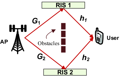
Figure 1: An RIS-aided multiuser MISO communication system.

II System Model

This paper investigates a RIS-aided MISO communication system as shown in Figure 1. The AP is equipped with $M$ antennas, and serves a single-antenna user. The direct transmission link between the AP and the user is blocked by the obstacles. In order to improve the propagation condition, $K$ RISs are deployed to provide high-quality virtual links from the AP to the user. Suppose each RIS has $N$ reflection elements. The baseband equivalent channels from the AP to the $k$-th RIS, and from the $k$-th RIS to the user at time slot $i$ are denoted by ${\bf G}_{k,i}\in{\mathbb{C}}^{N\times M}$ and ${\bf h}_{k,i}\in{\mathbb{C}}^{N\times 1}$, respectively. Then, the received signal at the user is expressed by

$${y_{i}}=\left(\sum_{k=1}^{K}{\bf h}_{k,i}^{\rm H}{\bf\Theta}_{k}{\bf G}_{k,i}\right){\bf w}_{i}s_{i}+u_{i},$$ (1)

where ${\bf\Theta}_{k}={\rm diag}(\vartheta_{1,k},\cdots,\vartheta_{n,k},\cdots,\vartheta_{N,k})$ is the diagonal phase-shift matrix of the $k$-th RIS with $\vartheta_{n,k}=e^{\jmath\varphi_{n,k}}$, $u_{i}\sim{\cal{CN}}(0,\sigma_{0}^{2})$ denotes the additive white Gaussian noise (AWGN) at the receiver, $s$ is the information-bearing signal at AP with unit power, and ${\bf w}_{i}\in{\mathbb{C}}^{M\times 1}$ is the corresponding transmit beamforming vector at the AP. We further define

$${{\bm{\theta}}}=\begin{bmatrix}{\rm diag}({\bf\Theta}_{1}^{\rm H})\\ \vdots\\ {\rm diag}({\bf\Theta}_{K}^{\rm H})\end{bmatrix},\;{{\bf H}_{i}}=\begin{bmatrix}{\rm diag}({\bf h}_{1,i}^{\rm H}){\bf G}_{1,i}\\ \vdots\\ {\rm diag}({\bf h}_{K,i}^{\rm H}){\bf G}_{K,i}\end{bmatrix}.$$

Then the received signal ${y_{i}}$ is equivalently represented by

$${y_{i}}={\bm{\theta}}^{\rm H}{\bf H}_{i}{\bf w}_{i}s_{i}+u_{i}.$$ (2)

According to [19], the optimal transmit beamforming can be expressed as the following function of ${\bf H}_{i}^{\rm H}{\bm{\theta}}$

$${\bf w}_{i}=\sqrt{P_{\rm T}}\frac{{\bm{\theta}}^{\rm H}{\bf H}_{i}}{\|{\bm{\theta}}^{\rm H}{\bf H}_{i}\|},$$ (3)

where $P_{\rm T}$ is the transmit power constraint. Therefore, the instantaneous achievable rate at time slot $i$ is

$$R_{i}({\bm{\theta}}) =\log\left(1+\frac{P_{\rm T}}{\sigma_{0}^{2}}{\left\|{\bm{\theta}}^{\rm H}{\bf H}_{i}\right\|^{2}}\right).$$ (4)

It is known that the passive RIS has no capability of channel estimation. In addition, the dimensions of ${\bf h}_{k,i}$ and ${\bf G}_{k,i}$ makes channel estimation very challenging, especially when $N$ is large. As a result, it is difficult to obtain the perfect knowledge of these channel coefficients in most practical cases. In this paper, we propose to design ${\bm{\theta}}$ only based on the statistical information of ${\bf h}_{k,i}$ and ${\bf G}_{k,i}$, and the optimization problem for the statistical CSI setup can be formulated as follows:

$${\mathcal{P}}{\text{(A)}}\quad\max_{\forall{\bm{\theta}}}\quad {\mathbb{E}}_{i}\left[R_{i}({\bm{\theta}})\right]$$

$${\bf s.t.}\quad |\theta_{n}|=1,\quad\forall n=1,\cdots,KN,$$

where ${\mathbb{E}}_{i}\left[R_{i}({\bm{\theta}})\right]$ is the expectation of $R_{i}({\bm{\theta}})$ over all time slot.

It should be noted that the above problem is independent of the statistical models of channels. Thus it is more general and practical than model-based studies in [14] and [15].

III Stochastic Successive Convex Approximation for Average Rate Maximization

Generally speaking, there are two main challenges to solve ${\mathcal{P}}{\text{(A)}}$. Firstly, similar to the perfect CSI-based studies in [6, 7, 8, 9, 10, 11, 12, 13], the non-convex unit-modulus constraint is intractable. Secondly, the objective function ${\mathbb{E}}_{i}\left[R_{i}({\bm{\theta}})\right]$ is non-convex, and usually cannot be denoted by closed-form expression.

To deal with these challenges, we design a stationary-solution-achieved algorithm for ${\mathcal{P}}{\text{(A)}}$ in this section. At first, we replace $\bm{\theta}$ by $\bm{\varphi}$ to make the unit-modulus constraint a convex form, where ${\theta}_{n}=e^{\jmath{\varphi}_{n}}$ and ${\bm{\varphi}}=[\varphi_{1},\cdots,\varphi_{NK}]^{\rm T}$. Then, the optimization for the non-convex objective function is addressed by the SSCA technique [16, 17].

III-A Optimization Variable Substitution

Replacing $\bm{\theta}$ by $\bm{\varphi}$, the rate expression becomes

$${\bar{R}}_{i}({\bm{\varphi}}) =\log\left(1+\frac{P_{\rm T}}{\sigma_{0}^{2}}{\left\|{\left(e^{\jmath{\bm{\varphi}}}\right)}^{\rm H}{\bf H}_{i}\right\|^{2}}\right).$$ (5)

Thus ${\mathcal{P}}{\text{(A)}}$ is translated to

$${\mathcal{P}}{\text{(A1)}}\quad\min_{\forall{\bm{\varphi}}}\quad f({\bm{\varphi}})=-{\mathbb{E}}_{i}\left[{\bar{R}}_{i}({\bm{\varphi}})\right]$$

$${\bf s.t.}\quad \varphi_{n}\in{\mathbb{R}},\quad\forall n=1,\cdots,KN.$$

Since the objective function is continuously differentiable with Lipschitz continuous gradient, ${\mathcal{P}}{\text{(A1)}}$ is the standard stochastic social optimization problem satisfying the applicable assumptions in [16].

III-B SSCA for ${\mathcal{P}}{\text{(A1)}}$

${\mathcal{P}}{\text{(A1)}}$ is still difficult to solve, since the objective function is non-convex with no closed-form expression. Fortunately, these issues can be dealt with SSCA technique. The key idea of the SSCA technique is first to approximate the gradient of $f({\bm{\varphi}})$ with a carefully-designed incremental sample estimate, and then linearize the non-convex part of $f({\bm{\varphi}})$ with the obtained gradient to render a convex surrogate objective function. Specifically, when the random realization ${\bf H}_{i}$ at time slot $i$ is obtained, ${\bm{\varphi}}$ is updated by the following three-step method:

• Firstly, we approximate the gradient of $f({\bm{\varphi}})$ with a incremental simple estimate. Define ${\bf f}^{(i)}$ and ${\bm{\varphi}}^{(i)}$ to be the approximated gradient and the obtained ${\bm{\varphi}}$ at time slot $i$, respectively. Then we have

  $${\bf f}^{(i)}=(1-\rho^{(i)}){\bf f}^{(i-1)}-\rho^{(i)}\nabla{R}_{i}({\bm{\varphi}}^{(i-1)}),$$ (6)

  where $\rho^{(i)}=i^{-\beta}$, $0.5\leq\beta\leq 1$, and $\nabla{R_{i}}({\bm{\varphi}})$ is the gradient of $R_{i}({\bm{\varphi}})$. According to the chain rule, we have

  $$\nabla{R}_{i}({\bm{\varphi}})={\rm Re}\left\{-\jmath{\bm{\theta}}^{\ast}\circ\nabla R_{i}({\bm{\theta}})\right\},$$ (7)

  where $\circ$ denotes the Hadamard product, ${\bm{\theta}}^{\ast}$ is the conjugate of ${\bm{\theta}}$, and define ${\bf A}_{i}=\frac{P_{\rm T}}{\sigma_{0}^{2}}{\bf H}(i){\bf H}(i)^{\rm H}$, we have

  $$\nabla R_{i}({\bm{\theta}})=\frac{2{\bf A}_{i}{\bm{\theta}}}{1+{\bm{\theta}}^{\rm H}{\bf A}_{i}{\bm{\theta}}}.$$ (8)

• Secondly, we find the incremental element of ${\bm{\varphi}}$ at time slot $i$. Based on the obtained ${\bf f}^{(i)}$, $f({\bm{\varphi}})$ is approximated by the following surrogate function:

  $${\hat{f}}_{i}({\bm{\varphi}},{\bm{\varphi}}^{(i-1)})=\langle{\bm{\varphi}}-{\bm{\varphi}}^{(i-1)},{\bf f}^{(i)}\rangle+\frac{\tau}{2}\|{\bm{\varphi}}-{\bm{\varphi}}^{(i-1)}\|^{2},$$

  where $\tau>0$, and $\langle{\bf x},{\bf y}\rangle$ is the inner product of vectors $\bf x$ and $\bf y$. Note that ${\hat{f}}_{i}({\bm{\varphi}},{\bm{\varphi}}^{(i-1)})$ is a convex function. Thus the incremental element can be obtained by solving the following convex optimization problem

  $${\hat{\bm{\varphi}}}=\arg\;\min_{\forall{\bm{\varphi}}}\; {\hat{f}}_{i}({\bm{\varphi}},{\bm{\varphi}}^{(i-1)}),$$

  and its closed-form expression is

  $${\hat{\bm{\varphi}}}={\bm{\varphi}}^{(i-1)}-\frac{{\bf f}^{(i)}}{\tau}.$$ (9)

• Finally, ${\bm{\varphi}}$ is updated by

  $${\bm{\varphi}}^{(i)}=(1-\gamma^{(i)}){\bm{\varphi}}^{(i-1)}+\gamma^{(i)}{\hat{\bm{\varphi}}},$$ (10)

  where $\gamma^{(i)}=i^{-\alpha}$, and we need $\beta<\alpha\leq 1$ to guarantee convergence [16].

We summarize the proposed algorithm in Algorithm 1. Despite the concise updating rules, the hyperparameter $\tau$ should be fine-tuned to realize a fast converge speed as well as a good performance, which requires extra off-line signal processing cost when the statistical CSI changes [16]. In the next section, we will proposed an online implementable method,which can obtain a sub-optimal solution.

Algorithm 1 SSCA for Average Rate Maximization.

1:  Initialize ${\bm{\varphi}}^{(0)}$ and $\epsilon$, and set ${\bf f}^{(0)}={\bf 0}$ and $i=0$.Repeat

2:  Obtain new channel realization ${\bf H}_{i}$;

3:  Update ${\bf f}^{(i)}$ according to (6);

4:  Solve ${\hat{\bm{\varphi}}}$ by (9);

5:  Let ${\bm{\varphi}}^{(i)}=(1-\gamma^{(i)}){\bm{\varphi}}^{(i-1)}+\gamma^{(i)}{\hat{\bm{\varphi}}}$;

6:  $i=i+1$; Until $\left|{\hat{f}}_{i}({\bm{\varphi}}^{(i)},{\bm{\varphi}}^{(i-1)})-{\hat{f}}_{i}({\bm{\varphi}}^{(i-1)},{\bm{\varphi}}^{(i-1)})\right|<\epsilon$.

IV Stochastic Majorization-Minimization for Average SNR Maximization

One can see that, the main design challenge to resolve ${\mathcal{P}}{\text{(A)}}$ is the logarithm function in $R_{i}({\bm{\theta}})$, which makes the objective function neither convex nor concave. In this section, a heuristic but implementation friendly algorithm is proposed, which approximates the average rate by the average received SNR. Specifically, we have following approximated problem:

$${\mathcal{P}}{\text{(B)}}\quad\min_{{\bm{\theta}}}\quad g({\bm{\theta}})\triangleq{\mathbb{E}}_{i}\left[g_{i}({\bm{\theta}})\right]$$

$${\bf s.t.}\quad |\theta_{n}|=1,\quad\forall n=1,\cdots,KN,$$

where $g_{i}({\bm{\theta}})={\bm{\theta}}^{\rm H}{\bf B}_{i}{\bm{\theta}}$, and ${\bf B}_{i}=-{\bf H}(i){\bf H}(i)^{\rm H}$. Although both the constraint set and the objective function of ${\mathcal{P}}{\text{(B)}}$ are still non-convex, we will show that the constraint set can be relaxed to the convex one equivalently, and then iterative algorithm with simple online-implementable updating rule for ${\mathcal{P}}{\text{(B)}}$ can be designed based on the SMM method [18].

IV-A Unit-Modulus Convex Relaxation

The objective function $g({\bm{\theta}})$ could be further written as

$$g({\bm{\theta}})={\bm{\theta}}^{\rm H}{\bar{\bf B}}{\bm{\theta}},$$ (11)

where ${\bar{\bf B}}={\mathbb{E}}_{i}\left[{\bf B}_{i}\right]$. Then, based on following proposition, the non-convex phase constraint can be relaxed.

Proposition 1

The optimization problem ${\mathcal{P}}{\text{(B)}}$ is equivalent to the following problem with convex constraint set:

$${\mathcal{P}}{\text{(B1)}}\quad\min_{{\bm{\theta}}}\quad g(\bm{\theta})$$

$${\bf s.t.}\quad |\theta_{n}|^{2}\leq 1,\quad\forall n=1,\cdots,KN.$$

Proof:

Since ${\bf B}_{i}=-{\bf H}(i){\bf H}(i)^{\rm H}$ is negative semidefinite, ${\bar{\bf B}}$ is also negative semidefinite, and $g(\bm{\theta})$ is concave. Therefore, in ${\mathcal{P}}{\text{(B1)}}$, the optimal $\theta_{n}$ is chosen at the boundary of the constraint set $|\theta_{n}|^{2}\leq 1$. ∎

Proposition 1 reveals the fact that, every element on the RIS should adopt the highest reflection strength to maximize the average (or instantaneous) SNR.

IV-B SMM for ${\mathcal{P}}{\text{(B1)}}$

SMM is an iterative algorithm to deal with the non-convex stochastic optimization problem like ${\mathcal{P}}{\text{(B1)}}$, which is the combination of the sample average approximation (SAA) method and the majorization-minimization (MM) method [20].

According to the SAA method, in the $t$-th time slot, the realization ${\bf B}_{t}$ is coming, and the output ${\bm{\theta}}^{(t)}$ is updated by solving:

$${\mathcal{P}}{\text{(B2)}}\quad{\bm{\theta}}^{(t)} =\arg\;\min_{{\bm{\theta}}}\;{\tilde{g}}_{t}({\bm{\theta}})\triangleq\frac{1}{t}\sum_{i=1}^{t}g_{i}({\bm{\theta}})$$

$${\bf s.t.}\quad |\theta_{n}|^{2}\leq 1,\quad\forall n=1,\cdots,KN.$$

Denote the SAA of ${\bf B}_{i}$ as follows:

$${\tilde{\bf B}}_{t}=\frac{1}{t}\sum_{i=1}^{t}{\bf B}_{i},$$ (12)

and then ${\tilde{g}}_{t}({\bm{\theta}})$ becomes

$${\tilde{g}}_{t}({\bm{\theta}})={\bm{\theta}}^{\rm H}{\tilde{\bf B}}_{t}{\bm{\theta}}.$$ (13)

However, since $g_{i}({\bm{\theta}})$ is non-convex, ${\tilde{g}}_{t}({\bm{\theta}})$ is non-convex as well, and ${\mathcal{P}}{\text{(B2)}}$ is challenge to solve. Fortunately, a stationary-solution achieved method has been proposed in [18] for this kind of problem, which is the stochastic extension version of the conventional MM method. In particular, stationary solution for ${\mathcal{P}}{\text{(B1)}}$ can be obtained by solving the following approximation problem iteratively:

$${\mathcal{P}}{\text{(B3)}}\quad{\bm{\theta}}^{(t)} =\arg\;\min_{{\bm{\theta}}}\;{\bar{g}}_{t}({\bm{\theta}})\triangleq\frac{1}{t}\sum_{i=1}^{t}{\hat{g}}_{i}({\bm{\theta}},{\bm{\theta}}^{(i-1)})$$

$${\bf s.t.}\quad |\theta_{n}|^{2}\leq 1,\quad\forall n=1,\cdots,KN.$$

where ${\hat{g}}_{i}({\bm{\theta}},{\bm{\theta}}^{(i-1)})$ is the surrogate function for $g_{i}({\bm{\theta}})$, which is uniformly strongly convex, and satisfies the MM constraint [20]:

$${\hat{g}}_{i}({\bm{\theta}},{\bm{\theta}})={g}_{i}({\bm{\theta}}),$$ (14a)

$${\hat{g}}_{i}({{\bm{\theta}}},{\bm{\theta}}^{(i-1)})\geq{g}_{i}({{\bm{\theta}}}).$$ (14b)

In the next, we first design surrogate function which satisfies (14a) and (14b). Then, updating rule is designed by solving ${\mathcal{P}}{\text{(B3)}}$.

IV-B1 Surrogate Function

Since ${\bf B}_{i}\preceq 0$, we have $\left({\bm{\theta}}-{{\bm{\theta}}^{(i-1)}}\right)^{\rm H}{\bf B}_{i}\left({\bm{\theta}}-{{\bm{\theta}}^{(i-1)}}\right)\leq 0$. Based on that, one may design surrogate function as follows:

$${\hat{g}}_{i}({\bm{\theta}},{{\bm{\theta}}^{(i-1)}}) ={{\bm{\theta}}^{(i-1)}}^{\rm H}{\bf B}_{i}{{\bm{\theta}}^{(i-1)}}-2{\rm Re}\left\{{{\bm{\theta}}^{(i-1)}}^{\rm H}{\bf B}_{i}{\bm{\theta}}\right\}$$ (15)

$$\qquad\qquad+\tau\|{\bm{\theta}}-{{\bm{\theta}}^{(i-1)}}\|^{2}.$$

Note that, equations (14a) and (14b) hold even though $\tau=0$. Thus we may set $\tau$ as an arbitrary small number to make ${\hat{g}}_{i}({\bm{\theta}},{\bm{\theta}}^{(i-1)})$ uniformly strongly convex.

IV-B2 Problem Decompose

Define ${\bf d}_{t}$ as the SAA of ${\bf B}_{i}{\bm{\theta}}^{(i-1)}$, which is updated recursively:

$${\bf d}_{t}=\frac{1}{t}{\bf B}_{t}{\bm{\theta}}^{(t-1)}+(1-\frac{1}{t}){\bf d}_{t-1}.$$ (16)

Then we have

$$\frac{1}{t}\sum_{i=1}^{t}{\rm Re}\left\{{{\bm{\theta}}^{(i-1)}}^{\rm H}{\bf B}_{i}{\bm{\theta}}\right\}={\rm Re}\left\{{\bf d}_{t}^{\rm H}{\bm{\theta}}\right\}.$$ (17)

Substituting (17) into ${\bar{g}}_{t}({\bm{\theta}})$, and removing the constant terms, ${\mathcal{P}}{\text{(B3)}}$ is equivalently written by

$${\mathcal{P}}{\text{(B3)}}\quad{\bm{\theta}}^{(t)} =\arg\;\min_{{\bm{\theta}}}\;{\ddot{g}}_{t}({\bm{\theta}})$$

$${\bf s.t.}\quad |\theta_{n}|^{2}\leq 1,\quad\forall n=1,\cdots,KN,$$

where ${\ddot{g}}_{t}({\bm{\theta}})=-2{\rm Re}\left\{{\bf d}_{t}^{\rm H}{\bm{\theta}}\right\}+\frac{1}{t}\sum_{i=1}^{t}\tau\|{\bm{\theta}}-{{\bm{\theta}}^{(t-1)}}\|^{2}$. In addition, ${\ddot{g}}_{t}({\bm{\theta}})$ can be further written by

$${\ddot{g}}_{t}({\bm{\theta}})=\sum_{n=1}^{NK}{\ddot{g}}_{n,t}({\theta_{n}}),$$ (18)

where ${\ddot{g}}_{n,t}({\theta_{n}})$ is the function of ${\theta_{n}}$:

$${\ddot{g}}_{n,t}({\theta_{n}})=-2{\rm Re}\left\{{d}_{n,t}^{\rm H}{\theta_{n}}\right\}+\frac{1}{t}\sum_{i=1}^{t}\tau\|{\theta_{n}}-{\theta_{n}^{(t-1)}}\|^{2},$$ (19)

and $d_{n,t}$ is the $n$-th element of ${\bf d}_{t}$. Therefore, based on (18), problem ${\mathcal{P}}{\text{(B3)}}$ can be decoupled into $KN$ subproblems with respect to each $\theta_{n}$:

$${\mathcal{P}}{\text{(B4)}}\quad\theta_{n}^{(t)} =\arg\;\min_{{\theta_{n}}}\;{\ddot{g}}_{n,t}({\theta_{n}})$$

$${\bf s.t.}\quad |\theta_{n}|^{2}\leq 1.$$

IV-B3 Updating Rule

${\mathcal{P}}{\text{(B4)}}$ is the convex optimization problem, which can be solved by the Karush-Kuhn-Tucker (KKT) conditions. Define the Lagrangian as

$${\cal L}(\theta_{n},\lambda)={\ddot{g}}_{n,t}({\theta_{n}})+\lambda(|\theta_{n}|^{2}-1)$$ (20)

where $\lambda\geq 0$. Then according to the KKT conditions, the optimal $\theta_{n}$ and $\lambda$ should satisfy

$$\nabla_{\theta_{n}}{\cal L}(\theta_{n},\lambda)=0,$$ (21a)

$$\lambda(|\theta_{n}|^{2}-1)=0.$$ (21b)

From (21a), the optimal solution of ${\mathcal{P}}{\text{(B4)}}$ given $\lambda$ is:

$$\theta_{n}^{(t)}=\frac{d_{n}+\tau{\ddot{\theta}}_{n}^{(t)}}{\tau+\lambda},$$ (22)

where ${\ddot{\theta}}_{n}^{(t)}$ is the SAA of $\theta_{n}^{(i-1)}$, which can also be learnt recursively:

$${\ddot{\theta}}_{n}^{(t)}=\frac{1}{t}\theta_{n}^{(t)}+(1-\frac{1}{t}){\ddot{\theta}}_{n}^{(t-1)}.$$ (23)

The rest task is to determine $\lambda$ based on (21b) and (22). Since we choose $\tau\approx 0$, when $\lambda=0$, constraint $|\theta_{n}|^{2}\leq 1$ does not hold. Thus we should have $|\theta_{n}|^{2}=1$. Finally, the optimal solution of ${\mathcal{P}}{\text{(B4)}}$ is:

$$\theta_{n}^{(t)}=e^{-\jmath\angle(d_{n}+\tau{\ddot{\theta}}_{n}^{(t)})}.$$ (24)

The above SMM based algorithm is summarized in Algorithm 2. Note that, although Algorithm 2 also has the parameter $\tau$, the performance and the convergence speed is not sensitive to the value of $\tau$, since equations (14a) and (14b) always hold for any $\tau$. Since no off-line fine-tuning is required, Algorithm 2 can be deployed online, meanwhile the statistical CSI is learnt from the incoming observations without any prior knowledge about the channel.

Algorithm 2 SMM for Average SNR Maximization.

1:  Initialize ${\bm{\theta}}^{(0)}$, and set $t=1$.Repeat

2:  Obtain new channel realization ${\bf B}_{t}$;

3:  Update ${\tilde{\bf B}}$, ${\bf d}_{t}$, and ${\ddot{\theta}}_{n}^{(t)}$ for all $n$ based on (12), (16), and (23), respectively;

4:  Update ${\bm{\theta}}^{(t)}$ according to (24).

5:  $t=t+1$; Until $\left|{\tilde{g}}({\bm{\theta}}^{(t)})-{\tilde{g}}({\bm{\theta}}^{(t-1)})\right|<\epsilon$.

V Numerical Results

In this section, numerical examples are provided to validate the effectiveness of the proposed algorithms. Suppose that the AP and the RISs are deployed properly, following [14], the channels between the AP and the RISs are modeled in Rician fading, i.e.,

$${\bf G}_{k}=\sqrt{\frac{\rho}{\rho+1}}{\bar{\bf G}}_{k}+\sqrt{\frac{1}{\rho+1}}{\tilde{\bf G}}_{k},$$

where ${\bar{\bf G}}_{k}$ and ${\tilde{\bf G}}_{k}$ are the LoS and NLoS components, respectively, $\rho=10$ is the Rician factor, and the elements of ${\tilde{\bf G}}_{k}$ are i.i.d. standard complex Gaussian distributed. Same as [14], we assume the multiple antennas at the AP and the reflector elements at the RIS are arranged in the uniform linear array (ULA) for simplicity. Then, the LoS components are expressed by the responses of the ULA:

$${\bar{\bf G}}_{k}={\bm{\alpha}}_{N}(\phi_{{\text{A}oA},k}){\bm{\alpha}}_{M}(\phi_{{\text{A}oD},k})^{\rm H},$$

where ${\bm{\alpha}}_{N}(\phi)=[1,e^{\jmath\pi\sin\phi},\cdots,e^{\jmath\pi(N-1)\sin\phi}]$, $\phi_{{\text{A}oA},k}$ is the AoA at the $k$-th RIS, and $\phi_{{\text{A}oD},k}$ is the AoD at the AP to the $k$-th RIS. We further assume that there are $L=5$ channel paths between the RIS and the user. Then, the channel vector ${\bf h}_{k}$ is expressed as

$${\bf h}_{k}=\sum_{l=1}^{L}\beta_{l,k}{\bm{\alpha}}_{N}(\phi_{l,k}),$$

where $\beta_{l,k}\sim{\cal{CN}}(0,\sigma_{\beta_{l,k}}^{2})$, and $\sigma_{\beta_{l,k}}^{2}$ is randomly generated from an exponential distribution and normalized by $\sum_{l=1}^{L}\sigma_{\beta_{l,k}}^{2}=1$. We set the transmission bandwidth as $200$ kHz and noise power spectral density as $-170$ dBm/Hz. In addition, suppose the distances between AP and RISs, and the distances between RISs and the user are the same, i.e., $d=10$ m. Then, the path loss is modeled by $38.46+20\lg d$ dB.

In simulation, we first generate $100$ snapshots, in which all the angles $\phi_{{\text{A}oA},k}$, $\phi_{{\text{A}oD},k}$ and $\phi_{l,k}$ are are randomly chosen from $(0,2\pi]$, and $\sigma_{\beta_{l,k}}^{2}$ is randomly generated from the exponential distribution and then normalized. Then, in each snapshot, we further generate $100$ independent realizations of small-scale fading ${\tilde{\bf G}}_{k}$ and $\beta_{l,k}$. We set $\epsilon=0.01$ as the stoping criterion for the proposed algorithms.

Figure 2 illustrates the average rate of different schemes with respect to the transmit power $P_{\rm T}$. One can see that, the proposed algorithms may achieve about $10$ dB gain compared with the random RIS phase scheme. In addition, Algorithm 1 and 2 achieve almost the same performance. Hence, optimizing the average received SNR is a good approximation to optimizing the average achievable rate, which is coincident with the conclusion in [14].

Then, in Figure 3, the total RIS element number $NK$ is fixed to $64$, and the average achievable rate is plotted for different $K$. Since each RIS has different $\phi_{{\text{A}oA},k}$, $\phi_{{\text{A}oD},k}$, and $\phi_{l,k}$, when $K$ increases, the performance of the random RIS phase scheme increases slightly due to the diversity gain. However, the performance of the statistical-CSI based schemes decreases drastically, since the number of the long-term variables required to be learnt increases proportionally to $K$. As a result, in practice, we think it is better to serve one user with only one RIS.

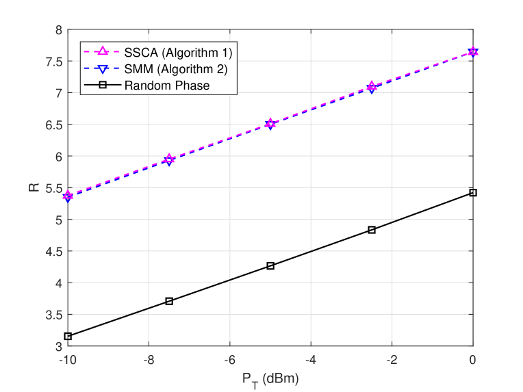
Figure 2: R versus $P_{\rm T}$, when $M=4$, $K=2$, and $N=20$.

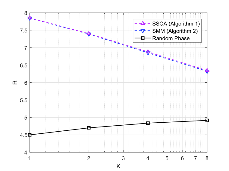
Figure 3: R versus $K$, when $M=4$, $P_{\rm T}=-5$ dB, and $NK=64$.

VI Conclusion

In this paper, we investigate the multiple-RIS-aided downlink MISO system. Two algorithms are developed to optimize the phase matrices of the RISs by exploiting the statistical CSI. Both algorithms are applicable for any channel model assumptions. Numerical results verify that the proposed algorithms may sufficiently outperform the random phase scheme, especially when $K$ is small.

References

• [1] C. Liaskos, S. Nie, A. Tsioliaridou, A. Pitsillides, S. Ioannidis, and I. Akyildiz, “A new wireless communication paradigm through software-controlled metasurfaces,” IEEE Commun. Mag., vol. 56, no. 9, pp. 162–169, 2018.
• [2] E. Basar, M. Di Renzo, J. de Rosny, M. Debbah, M.-S. Alouini, and R. Zhang, “Wireless communications through reconfigurable intelligent surfaces,” arXiv preprint arXiv:1906.09490, 2019.
• [3] Q. Wu and R. Zhang, “Towards smart and reconfigurable environment: Intelligent reflecting surface aided wireless network,” arXiv preprint arXiv:1905.00152, 2019.
• [4] Y.-C. Liang, R. Long, Q. Zhang, J. Chen, H. V. Cheng, and H. Guo, “Large intelligent surface/antennas (LISA): Making reflective radios smart,” J. Commun. Inf. Netw., vol. 4, no. 2, pp. 40–50, June 2019.
• [5] Q.-U.-A. Nadeem, A. Kammoun, A. Chaaban, M. Debbah, and M.-S. Alouini, “Intelligent reflecting surface assisted multi-user MISO communication,” arXiv preprint arXiv:1906.02360, 2019.
• [6] Q. Wu and R. Zhang, “Intelligent reflecting surface enhanced wireless network: Joint active and passive beamforming design,” in Proc. IEEE Globecom, Dec. 2018, pp. 1–6.
• [7] ——, “Intelligent reflecting surface enhanced wireless network via joint active and passive beamforming,” arXiv:1809.01423, 2018.
• [8] C. Huang, A. Zappone, M. Debbah, and C. Yuen, “Achievable rate maximization by passive intelligent mirrors,” in Proc. IEEE ICASSP, May. 2018, pp. 3714–3718.
• [9] C. Huang, A. Zappone, G. C. Alexandropoulos, M. Debbah, and C. Yuen, “Reconfigurable intelligent surfaces for energy efficiency in wireless communication,” IEEE Trans. Wireless Commun., vol. 18, no. 8, pp. 4157–4170, 2019.
• [10] H. Guo, Y.-C. Liang, J. Chen, and E. G. Larsson, “Weighted sum-rate optimization for intelligent reflecting surface enhanced wireless networks,” arXiv preprint arXiv:1905.07920, 2019.
• [11] C. Pan, H. Ren, K. Wang, W. Xu, M. Elkashlan, A. Nallanathan, and L. Hanzo, “Intelligent reflecting surface for multicell MIMO communications,” arXiv preprint arXiv:1907.10864, 2019.
• [12] M. Cui, G. Zhang, and R. Zhang, “Secure wireless communication via intelligent reflecting surface,” IEEE Wireless Commun. Lett., to be published.
• [13] J. Chen, Y.-C. Liang, Y. Pei, and H. Guo, “Intelligent reflecting surface: A programmable wireless environment for physical layer security,” IEEE Access, vol. 7, pp. 82 599–82 612, 2019.
• [14] Y. Han, W. Tang, S. Jin, C. Wen, and X. Ma, “Large intelligent surface-assisted wireless communication exploiting statistical CSI,” IEEE Trans. Veh. Technol., vol. 68, no. 8, pp. 8238–8242, 2019.
• [15] Q.-U.-A. Nadeem, A. Kammoun, A. Chaaban, M. Debbah, and M.-S. Alouini, “Large intelligent surface assisted MIMO communications,” arXiv:1903.08127, 2019.
• [16] Y. Yang, G. Scutari, D. P. Palomar, and M. Pesavento, “A parallel decomposition method for nonconvex stochastic multi-agent optimization problems,” IEEE Trans. Signal Process., vol. 64, no. 11, pp. 2949–2964, 2016.
• [17] A. Liu, V. K. N. Lau, and M. Zhao, “Online successive convex approximation for two-stage stochastic nonconvex optimization,” IEEE Trans. Signal Process., vol. 66, no. 22, pp. 5941–5955, 2018.
• [18] M. Razaviyayn, M. Sanjabi, and Z.-Q. Luo, “A stochastic successive minimization method for nonsmooth nonconvex optimization with applications to transceiver design in wireless communication networks,” Mathematical Programming, vol. 157, no. 2, pp. 515–545, 2016.
• [19] D. Tse and P. Viswanath, Fundamentals of wireless communication.   Cambridge university press, 2005.
• [20] Y. Sun, P. Babu, and D. P. Palomar, “Majorization-minimization algorithms in signal processing, communications, and machine learning,” IEEE Trans. Signal Process., vol. 65, no. 3, pp. 794–816, 2017.