Well Temperaments based on the Werckmeister definition
From Werckmeister, passing Vallotti, Bach and Kirnberger,
to Equal Temperament.
Inspired by Kelletat and Amiot

Abstract

Mathematical steps are developed to obtain optimised well tempered model “temperaments”, based on a musical Well Temperament definition by H. Kelletat, that is derived from A. Werckmeister. This supports objective mathematical ranking of historical temperaments. Historical temperaments that fit best with mathematical models are often installed on organs. Musical appreciation and mathematical ranking of historical temperaments are in agreement. The diatonic C-major impurity of Well Temperaments lies between that of an elaborated optimal model and that of Equal Temperament. Historical Well Temperaments join these limits very closely and the list is amply filled in small rising steps. Hence, it achieves little to develop new Well Temperaments.
The developed RMS computing modules can also be used for precise and accurate recognition of historical temperaments.

Online Supplement: Spreadsheet with calculations and solutions

“Ce qui se conçoit bien s’énonce clairement, et les mots pour le dire arrivent aisément.”

(Boileau-Despréaux, 1674)

1 Issue

Ever since Antiquity, temperaments are a subject of discussion. Well Temperaments (WT) emerged in the 17-th century. Many differing WT are applied, but none is universally accepted. Musical WT criteria are pretty hard to translate into comprehensive objective evaluations or classification (Hall, 1973, pp. 274-290). All this results in the fact that the choice of a musical temperament remains part of the artistic freedom of musicians.

A novel and objective WT evaluation is proposed, by comparing historical WT with mathematically optimised WT models, with minimum diatonic impurity for C-major; the impurity being calculated according to

$$RMS_{Diatonic\ impurity}=\sqrt{\frac{\sum_{Weighted}(\mathrm{C}\mathrm{-}\mathrm{major}\ diatonic\ thirds\ \mathrm{and}\ fifths\ impurities)^{2}}{\sum(weights\ of\ intervals)}}$$ (1)

followed by a similar optimisation for fifths outside the diatonic C-major.

1.1 Well Temperaments

The German term for Well Temperament is “Wohltemperiert”. First Wohltemperiert use in writing was probably by Werckmeister A. (1681, title page), see fig.1 (Norback, 2002, p. 18), and was also used later (1686; 1689; 1698).

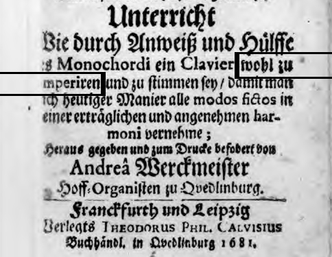
Figure 1: Orgelprobe 1681

Werckmeister’s WT requirements are still accepted and referred to nowadays (Norback, 2002, pp. 25-26). The Werckmeister III temperament became widespread and famous. The “Wohltemperiert” term probably became popular, for it was used in the title of “Das Wohltemperirte Clavier” (Bach J. S. 1722). It should however be noticed, that the musical education of J. S. Bach was based on meantone (Kelletat, 1981, p. 21, lines 3 to 9). F. Marpurg (1776, pp. 210-223; §§ 227-237) published an opinion, rejected by J. Kirnberger, -a student and follower of J. S. Bach- (Kelletat, 1981, p. 42), that J. S. Bach used the equal temperament. This opinion became widely published, copied, and accepted. The assumed WT and 12TET equivalence and 12TET practice by J. S. Bach, was only rejected in modern times; probably first by B. Bosanquet (1876, pp. 29-30), and only much later, again but thoroughly, by H. Kelletat (1957; 1960), which led to a breakthrough. Werckmeister’s publications have lead to a musical WT definition elaborated by H. Kelletat (1981, page 9, first paragraph):

WT means a mathematical-acoustic and musical-practical organisation of the tone system within the twelve steps of an octave, so that impeccable performance in all tonalities is enabled, based on the extended just intonation (natural-harmonic tone system), while striving to keep the diatonic intervals as pure as possible.

While tied to given pitch ratios, this temperament occurs as a thriftily tempered smoothing and extension of the meantone, as unequally beating semitonics and as equal (equally beating) temperament.

Later on many assumptions are made and published, about what has come to be called “Bach temperaments”; mathematical proposals arise also, about how to assess or create WT (Kellner, 1977; Goldstein, 1977; Sankey, 1997; Polansky, 2008; Amiot, 2010; Farup, 2013; Liern, 2015). This paper is mainly in line with Polansky, on which basis further numerical investigations and temperament comparisons are worked out.

1.1.1 Further Well Temperament key characteristics

From a collection of over one hundred historical temperaments, thirty one were filtered as WT and included in table 8, based on following criteria:

Major thirds

Almost unanimous historical assessments set the following ratio condition

$$1.25<\mathrm{Major\ third}<1.265625\ (=81/64=\mathrm{Pythagorean\ third})$$ (2)

Compare with: the just third $(5/4=1.25)$ or 12-TET third ($2^{4/12}$=1.2599…).

Fifths

Historical assessments of Kirnberger I and II set a lower limit on fifths (Kelletat, 1982, p. 34, lines 17 to 27): the discussed fifth has a ratio of 1.491.

$$1.491<fifth<1.509\quad\mathrm{values\ retained\ in\ this\ paper}$$ (3)

The associated upper limit is derived from the lower limit: it has the same beat. Some WT have fifth deviations up to one third of a comma. This leads to narrower limits, not retained here: as many as possible complying WT temperaments are desired.

1.2 Diatonic intervals: …“based on the extended just intonation”; … …“keep the diatonic intervals as pure as possible” …

In addition to obligate perfect primes and octaves, the most important musical intervals are fifths with perfect ratio of 3/2, major and minor thirds with just ratio of 5/4 and 6/5 respectively, and their inversions. These intervals constitute the backbone of the extended just intonation, building the diatonic C-major scale, also interconnecting all altered notes; see fig. 2.

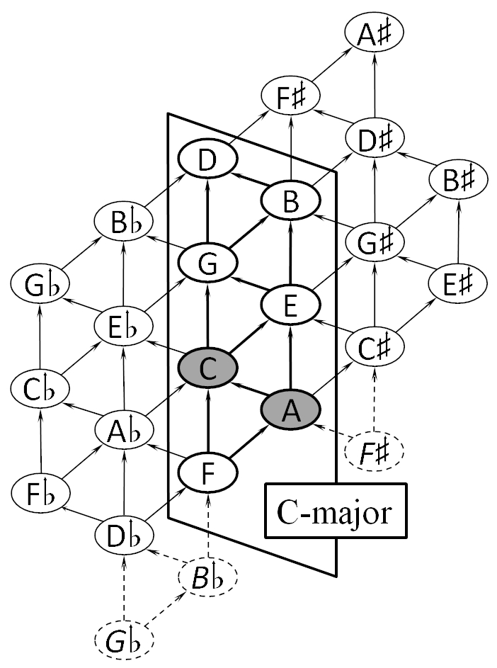
Figure 2: C-major diatonic structure

This structure is not deformable: all triangle sides have the fixed invariable value of a perfect or just interval.

This diatonic C-major scale contains undesired impurity on the D-F third and the D-A fifth (see also footnote 5). There are some more impure intervals on those containing altered notes. A combination of enharmonics on a single key is wanted for keyboard instruments. Optimisation of intervals is desirable, …and possible.

1.3 Interval impurity measurement: …“keep the diatonic intervals as pure as possible” …

A mathematical interval impurity measurement is required.
Music consists of periodic sounds. J. Fourier (1768-1830) developed mathematical evidence that any periodic function $F(t)$ consists of a sum of sine waves, -the harmonics-, whereby the sine wave frequencies are integer multiples of a basic frequency.

$F(t)=\sum\limits_{n=0}^{\infty}[a_{n}\sin{(2\pi nft)}+b_{n}\sin{(2\pi nft)]}\quad\mathrm{with}\ n=integer\ \mathrm{and\ with:}$

$$a_{n}=2f\int_{-1/2f}^{1/2f}F(t)\sin(2\pi nft)dt\quad\mathrm{and}\quad b_{n}=2f\int_{-1/2f}^{1/2f}F(t)\cos(2\pi nft)dt$$ (4)

A small musical interval impurity leads to a beating sound, because of the summation of mutual note harmonics, of almost equal frequency. For example: the beating of an imperfect fifth -ratio $\approx 3/2$-, mainly results from the sum of the second harmonic of the upper note with the third harmonic of the lower note, -but also from any higher harmonic 2n with any mutual higher harmonic 3n-. Fig. 3 displays the effect.

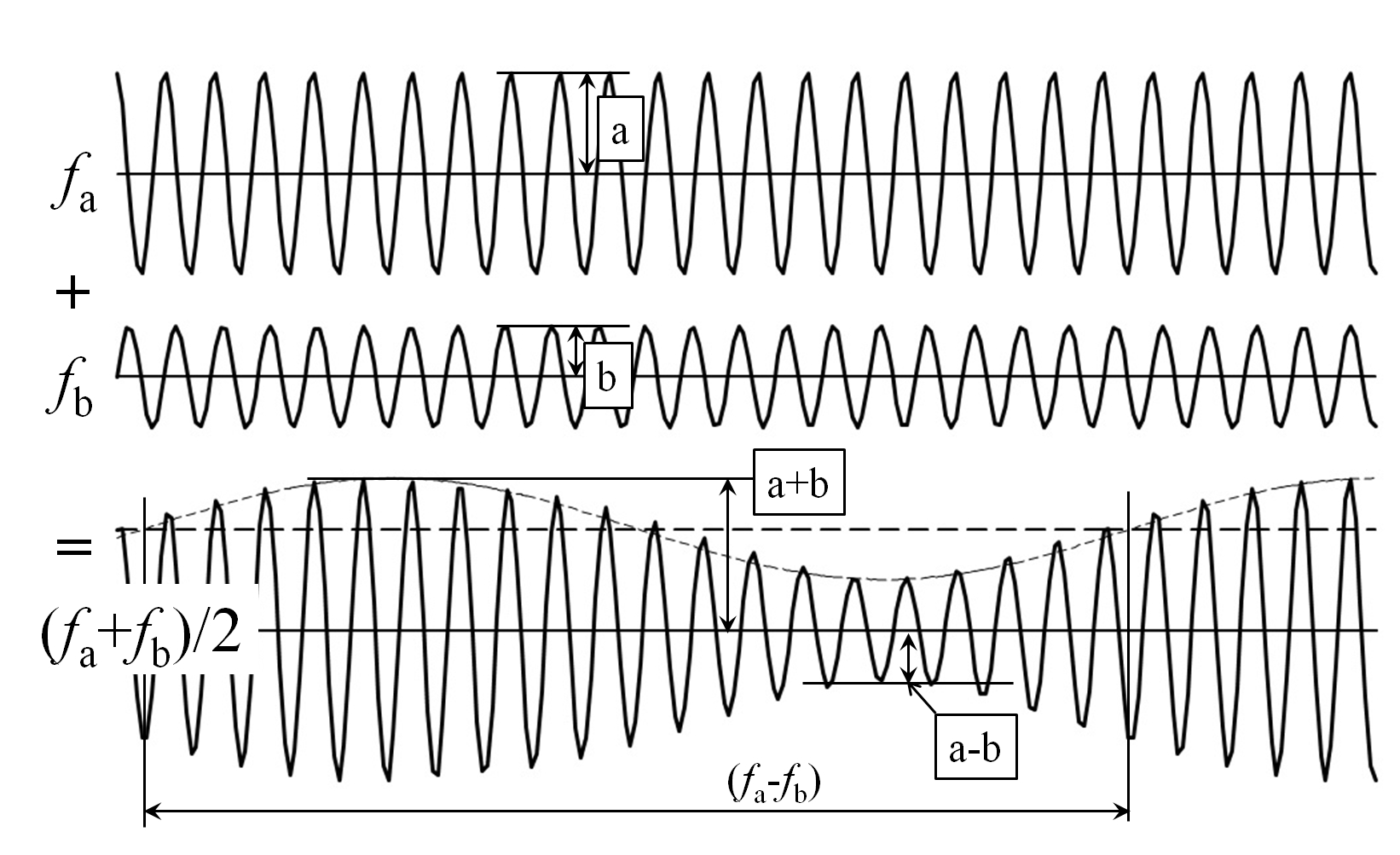
Figure 3: Beating of a musical interval

The sum of two sine waves is worked out in formula 5.

$$a\sin(2\pi f_{a}t)+b\sin(2\pi f_{b}t)=\sqrt{a^{2}+b^{2}+2ab\cos 2\pi(f_{a}-f_{b})t}\sin\left(2\pi\frac{f_{a}+f_{b}}{2}t\right)$$ (5)

Hence, this sum corresponds to a single sine wave:

• of median frequency $(f_{a}+f_{b})/2$

• with amplitude varying from $(a-b)$ to $(a+b)$, at modulation frequency $(f_{a}-f_{b})$

The lowest beat pitch of a fifth can therefore be set as.

$Beat_{fifth}=2f_{upper\ note}-3f_{lower\ note}=p_{1}f_{2}-p_{2}f_{1}$

This impurity measurement has been applied already, among others also by A. Kellner (1977). Alternate impurity measurements that can be thought of, are, for example

Beat $$= (p_{1}f_{2}-p_{2}f_{1})\ \mathrm{cps}\qquad\mathrm{Beat\ Pitch\ (cycles\ per\ second)}$$ (6)

PBP $$= 100(p_{1}f_{2}/f_{1}-p_{2})\ \mathrm{\%}\qquad\mathrm{Percentage\ Beat\ Pitch}$$ (7)

PPD $$= 100(p_{1}f_{2}/p_{2}f_{1}-1)\ \mathrm{\%}\qquad\mathrm{Pitch\ Purity\ Deviation}$$ (8)

Cents $$= 1200\log(p_{1}f_{2}/p_{2}f_{1})/\log 2\ \mathrm{cents}\qquad\mathrm{Pitch\ Purity\ Deviation\ in\ cents}$$ (9)

$$\mathrm{For\ low\ interval\ impurities\ we\ can\ set:}\qquad p_{1}f_{2}/{p_{2}f_{1}}\approx 1\qquad\mathrm{hence}$$ (10)

$$\log{\left(\frac{p_{1}f_{2}}{p_{2}f_{1}}\right)}\approx\frac{p_{1}f_{2}}{p_{2}f_{1}}-1=\frac{p_{1}f_{2}-p_{2}f_{1}}{p_{2}f_{1}}=\frac{p_{1}f_{2}-p_{2}f_{1}}{C_{1}^{t}}=\frac{p_{1}f_{2}/f_{1}-p_{2}}{C_{2}^{t}}$$ (11)

$$\mathrm{or}\qquad Cents\sim\mathrm{PPD}\sim\frac{p_{1}f_{2}-p_{2}f_{1}}{p_{2}f_{1}}\sim Beat/C_{1}^{t}\sim PBP/C_{2}^{t}$$ (12)

Impurity measurement differences are of second order only, hence, choice of measurement can be free: see for example in last paragraph, Appendix B.2.2, table 13, comparing Beat and Cent results. The preferred measurement for model elaborations in this paper is the Beat. It is an audible and direct acoustical sound, monitored for aural tuning. Cents will be used for model and temperament comparisons. Comparisons will therefore not depend on the chosen diapason, as a result of measurements based on ratios.

1.4 Considerations about the application of BEAT Impurity Measurements

1.4.1 Dependence on the pitch of the lower note

The allowed interval beat depends on the lower note pitch.
As for aural tuning, it can be said: the higher the lower note of an interval, the higher the allowed beat pitch (Plomp and Levelt, 1965, see: “C. Discussion”). If more intervals of equal type appear in a formula, the beat pitches should therefore be adapted by a factor inversely proportional to the pitch of the lower note, -for example the factor $2^{‒n/12}$-, according table 1.

Note	C	C$\sharp$	D	E$\flat$	E	F
Weight value	$2^{-0/12}$	$2^{-1/12}$	$2^{-2/12}$	$2^{-3/12}$	$2^{-4/12}$	$2^{-5/12}$
Weight symbol	$P_{C}$	$P_{C\sharp}$	$P_{D}$	$P_{E\flat}$	$P_{E}$	$P_{F}$
Note	F$\sharp$	G	G$\sharp$	A	B$\flat$	B
Weight value	$2^{-6/12}$	$2^{-7/12}$	$2^{-8/12}$	$2^{-9/12}$	$2^{-10/12}$	$2^{-11/12}$
Weight symbol	$P_{F\sharp}$	$P_{G}$	$P_{G\sharp}$	$P_{A}$	$P_{B\flat}$	$P_{B}$

Table 1: Note weights applicable with Beat impurity measurements

1.4.2 Obtained precisions of Note Pitches

The proposed note weights, table 1, lead to small errors: these weights deviate from the required exact value, except for the 12TET.
This error can be reduced by repeating the calculation, with weights derived from a preceding calculation. Two to three iterations will lead to a pitch precision better than the third decimal digit.
The iterations were applied whenever possible. Pitch corrections turned out to be very low, as expected, based on very small differences between proposed weights, table 1, and exact weights.

1.4.3 Beat - PBP equivalence

The proposed iterations, § 1.4.2, lead to equal pitch values as with PBP measurements, formula 7. It is an easy way to obtain analytic PBP solutions: the analytic method developed further in § 2.2.1, leads for PBP indeed, to a set of complex non linear equations.

1.5 Dependence on the type of interval

It is known from musical practice, that perfect fifths capture more attention than just thirds. This can be expressed mathematically, by assigning differing weights to fifths (weight:$P_{Fi}$), major thirds $(P_{MT})$, and minor thirds $(P_{mt})$. Because of fifths importance, their weights will always be set at $P_{Fi}=1$, -this weight factor will therefore not appear in formulas-, and the thirds weights will always have to be restricted to $0\leq P_{MT}$;$P_{mt}\leq 1$.

1.6 Impact of deviations from perfect or just ratios

Square impurity values offer some advantages for impurity evaluations:

• Musical

  • Musical impurities above an average impurity have to a certain extent more arithmetic impact, if the square of impurities is applied, see fig. 4. This corresponds to some degree with the musical impact on audience (Hall, 1973).

  • The square of impurities avoids a distinction between the sign of deviations, as is the case also for musical audience (Plomp and Levelt, 1965; Setshares, 1993). Attention: the sign is important for aural tuning.

    

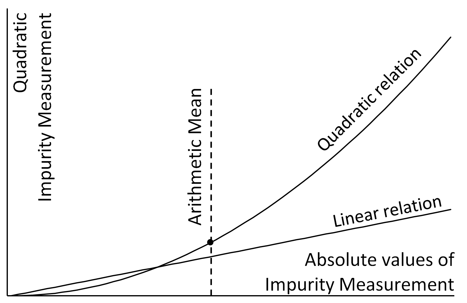
    Figure 4: Impact of squares

• Mathematical: for sets of intervals with equal arithmetic mean impurity, the -lower quality- set with larger deviations from the mean, has the largest RMS.

Further thoughts on measurements based on interval ratio measurement (PBP, PPD, Cents; formulas 7-9): see Appendix B.

2 Elaboration of Optimal Models

2.1 Impurity Formulas

Based on concerns of § 1, formulas below can be set ($P_{Note}$: see table 1).

Major thirds impurities:	Fifths impurities
C: $\Delta MT_{C}=(4E-5C)P_{C}$	C: $\Delta Fi_{C}=(2G-3C)P_{C}$
F: $\Delta MT_{F}=(4A-5F)P_{F}$	D: $\Delta Fi_{D}=(2A-3D)P_{D}$
G: $\Delta MT_{G}=(4B-5G)P_{G}$	E: $\Delta Fi_{E}=(2B-3E)P_{E}$
minor thirds impurities:	F: $\Delta Fi_{F}=(4C-3F)P_{F}$
D: $\Delta mt_{D}=(5F-6D)P_{D}$	G: $\Delta Fi_{G}=(4D-3G)P_{G}$
E: $\Delta mt_{E}=(5G-6E)P_{E}$	A: $\Delta Fi_{A}=(4E-3A)P_{A}$
A: $\Delta mt_{A}=(10C-6A)P_{A}$	B: A diatonic fifth on B does not exist:
B: $\Delta mt_{B}=(10D-6B)P_{B}$	a perfect fifth on B leads indeed to F$\sharp$

Table 2: Diatonic C-major impurities

See table 3 for the altered notes, outside the diatonic C-major.

C$\sharp$: $\Delta Fi_{C\sharp}=(2G\sharp-3C\sharp)P_{C\sharp}$	G$\sharp$: $\Delta Fi_{G\sharp}=(4Eb-3G\sharp)P_{G\sharp}$
E$\flat$: $\Delta Fi_{E\flat}=(2B\flat-3E\flat)P_{E\flat}$	B$\flat$: $\Delta Fi_{B\flat}=(4F-3B\flat)P_{B\flat}$
F$\sharp$: $\Delta Fi_{F\sharp}=(4C\sharp-3F\sharp G)P_{F\sharp}$	B: $\Delta Fi_{B}=(4F\sharp-3B)P_{B}$

Table 3: Impurities of fifths containing an altered note

An optimal diatonic C-major impurity elaboration by minimisation of formula 1, including preset weights $P_{MT}$ and $P_{mt}$, corresponds with the minimisation of

$$P_{MT}\sum{\Delta MT_{C,F,G}^{2}}+P_{mt}\sum{\Delta mt_{D,E,A,B}^{2}}+\sum{\Delta Fi_{C,D,E,F,G,A}^{2}}$$ (13)

and with F and B solved, the minimisation of

$$\sum{\Delta Fi_{C\sharp,E\flat,F\sharp,G\sharp,B\flat,B}^{2}}$$ (14)

2.2 Elaboration of models

2.2.1 First Model

A minimum or maximum of formula 13 can be obtained by setting the partial derivatives of the expression to zero, and solving the obtained set of linear equations.
Example: the partial derivative by C set to zero, of the expression formula 13, leads to

$\frac{\partial}{\partial C}\mathrm{:}\qquad(25P_{MT}P_{C}^{2}+100P_{mt}P_{A}^{2}+9P_{C}^{2}+16P_{F}^{2})C$

$$-20P_{MT}P_{C}^{2}E-12P_{F}^{2}F-6P_{C}^{2}G=60P_{mt}P_{A}^{2}A$$ (15)

The full set of equations, including those for altered notes, is available in Appendix A.1, and can be solved by means of a spreadsheet. Separate cells for entry of the $P_{MT}$ and $P_{mt}$ weights are recommended, to enable investigations on their impact. Separate matrices for denominator, and numerators allow for direct calculation and display of all results: pitches, impurities, graphs, comparisons, …
A spreadsheet with the solution of the set of equations is available for downloading. Fig. 5 displays the domain of weighted C-major diatonic impurities for $0\leq(P_{MT};P_{mt})\leq 1$.

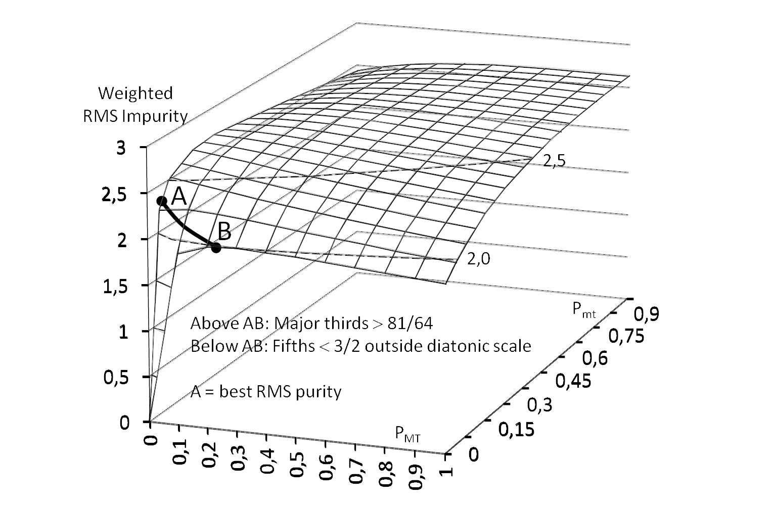
Figure 5: Weighted Diatonic Impurity as $F(P_{MT};P_{mt})$

Results on the A-B line

The A-B line separates a WT domain on and below the line, from a non-WT domain holding major thirds in excess of the Pythagorean ratio. $P_{MT}$ and $P_{mt}$ values in table 4 correspond with points on this line. This corresponds with B and F values resulting from six perfect fifths; those on B, F$\sharp$, C$\sharp$, G$\sharp$, E$\flat$, B$\flat$ (thus for $B/F=2^{10}/3^{6}$).
Point A has the best fifths, and B the best diatonic purity.

	Point A				Point B
Beat-RMS	2.364	2.266	2.172	2.077	1.988
Fifths	1.872	1.875	1.884	1.889	1.905
$P_{mt}$	0.05993	0.044	0.029	0.014	0.000
$P_{MT}$	0.000	0.050	0.100	0.150	0.20364

Table 4: Weighted Diatonic Impurity / Unweighted Fifths Impurity

Models on the A-B line are almost equivalent (see pitches, table 5).

	C	C$\sharp$	D	E$\flat$	E	F
Beat-WT-A	262.99	277.43	294.26	312.11	329.25	351.12
Beat-WT-B	263.06	277.49	294.32	312.18	329.30	351.20
	F$\sharp$	G	G$\sharp$	A	B$\flat$	B
Beat-WT-A	369.91	393.59	416.14	440.00	468.16	493.21
Beat-WT-B	369,99	393.76	416.24	440.00	468.27	493.32

Table 5: Beat-WT-A and Beat-WT-B

Domain below the A-B line $(B/F>2^{10}/3^{6})$

The limit ($P_{MT}=P_{mt}=0$) has perfect fifths within the diatonic C-major scale, all other fifths being slightly reduced. This ultimate corresponds to a best diatonic scale at altered notes, instead of at the diatonic C-major, which certainly is not the aim. The models are WT indeed, but not optimal, since best thirds purities have shifted towards altered notes. This shift can be avoided by imposing the A-B line condition in formula 13; this is by substituting B by $F\times 2^{10}/3^{6}$. It opens up new and wider possibilities for exploration of possible diatonic C-major interval optimisation; see further § 2.2.2.

Domain above the A-B line $(B/F<2^{10}/3^{6})$

It has been found that WT models within this domain are possible, without inducing major thirds with ratio exceeding the Pythagorean one, by setting specific conditions on some thirds. The corresponding optimal WT model is part of an unexplored WT domain with extreme diatonic major thirds purity, specific enlarged fifths, and unweighted diatonic purity =3.184. More details are given in Appendix A.3, and explain why this model is not withheld as the optimal model in temperament rankings (at tables 8 and 9).

2.2.2 Domain for $B=kF$, with $k=2^{10}/3^{6}$

Further diatonic C-major optimisation is possible substituting $B$ by $kF$, and applying the same method as in § 2.2.1. The modified partial derivatives of the sum of the modified squares formula 13, are given in Appendix A.2 to this paper.

With F solved, altered notes can be calculated more easily, based on their perfect fifths ratio, instead of solving the formula 14.

The domain of solutions is displayed in fig. 6. The minimum impurity is obtained at ($P_{MT}=P_{mt}=0$), with a weighted diatonic purity equal to 1.778; this model is identical to the historical Vallotti temperament.

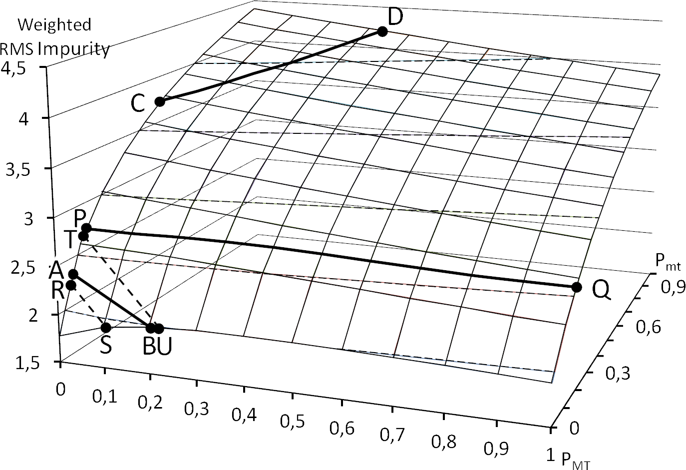
Figure 6: Diatonic Impurity as $F(P_{MT}$; $P_{mt}$)

A spreadsheet with solution can be downloaded.

Plenty of combinations of $P_{MT}$ and $P_{mt}$ are possible, but solutions above the C-D line, for ($P_{MT}$; $P_{mt}$) from (0; 0.466) to (0.357; 1), are not WT, because of major thirds exceeding the 81/64 ratio. The almost free choice of $P_{MT}$ and $P_{mt}$ values allows for investigation on which combination might be preferred, taking additional considerations into account, on top of the calculated and desired optimal diatonic C-major impurity. Following musical considerations make sense:

• Maintain the C-major diatonic fifths as close as possible to the perfect ratio

• Achieve a good balance between thirds and fifths impurities

These two points above, require insight into the course of the impurity contributions of thirds and fifths.
Those group contributions can be investigated by means of formulas 16.

$$RMS_{MT;mt}=\sqrt{\frac{\sum{(\Delta MT_{C,F,G}^{2}+\Delta mt_{D,E,A,B}^{2})}}{13}}\mathrm{;}\ RMS_{Fi}=\sqrt{\frac{\sum{\Delta Fi_{C,D,E,F,G,A}^{2}}}{13}}$$ (16)

The thirds impurities have a monotone continuous decrease from point $(P_{MT}=P_{mt}=0)$ to $(P_{MT}=P_{mt}=1)$; the fifths have an opposite evolution; see fig 7.

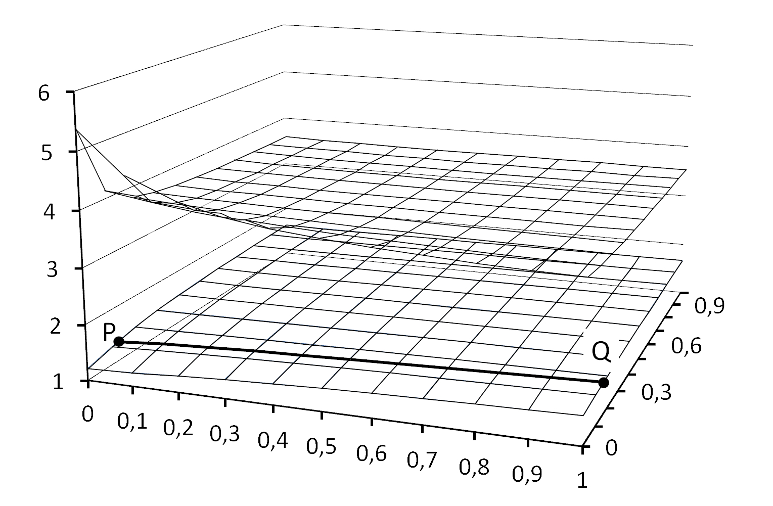
Figure 7: Course of unweighted diatonic thirds and fifths

Because of this opposition, some kind of balance should be possible between those two points, but lack of intersection of planes in fig. 7 reveals that some weighting of fifths and thirds impurity contributions is necessary.

A weighting balance is proposed, by introducing weights in formula 16; this corresponds with a dissociation of thirds and fifths contributions within formula 1; see formula 17.

$$\sqrt{\frac{P_{MT}\times\sum{\Delta MT_{C,F,G}^{2}}+P_{mt}\times\sum{\Delta mt_{D,E,A,B}^{2}}}{3P_{MT}+4P_{mt}+6}}=\sqrt{\frac{\sum{\Delta Fi_{C,D,E,F,G,A}^{2}}}{3P_{MT}+4P_{mt}+6}}$$ (17)

Any other balancing proposal based on rational considerations and objectivity should be acceptable.
The course of weighted thirds and fifths purities, based on the proposal of formula 17, is displayed in fig. 8.

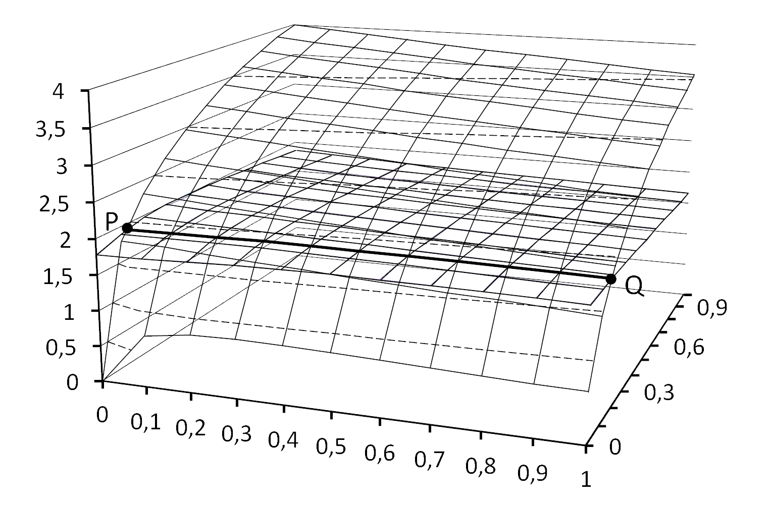
Figure 8: Course of weighted diatonic thirds and fifths

The most curved plane displays the thirds impurities. The P-Q line displays the collection of weights leading to equal impurity contribution of thirds and fifths (this line is also displayed in figures 6 and 7). Some numeric figures corresponding with this P-Q line are displayed in table 6.

Fifths Impurity	1.3481	1.4221	1.4704	1.5059	1.5334	1.5555
Diatonic Impurity	4.2928	4.1030	4.0257	3.9859	3.9630	3.9488
Weighted Diatonic Impurity	2.7024	2.7148	2.6874	2.6457	2.5982	2.5486
$P_{mt}$	0.1177	0.1335	0.1457	0.1557	0.1640	0.1710
$P_{MT}$	0.0	0.2	0.4	0.6	0.8	1.0

Table 6: Impurities of Fifths and the C-major diatonic scale

A best fifths purity combined with a thirds to fifths balance, can be observed at point P (for $P_{MT}=0$ table 6). The best fifths impurity is 13.3% smaller than the worst one, for a diatonic impurity increase of 8.7% only (6% weighted). Because of fifths purity importance, the point P is preferred: fifths purity is directly audible, indeed; musical evaluation of thirds or diatonic purity is difficult (see further, footnote 12, items (1) and (3)). Pitches of this model, named Beat-WT, are on display in table 7.

Beat-WT	C	C$\sharp$	D	E$\flat$	E	F
Piches	263.23	277.55	294.39	312.25	329.25	351.28
Beat-WT	F$\sharp$	G	G$\sharp$	A	B$\flat$	B
Pitches	370.07	393.95	416.33	440.00	468.37	493.43

Table 7: impurity = 2.7024; (4.2928 unweighted) Beat-WT $P_{MT}=0$; $P_{mt}=0.1177$

3 Evaluation and Comparison of Models and Historical WT

Most data on historical temperaments were obtained from Kelletat (1981; 1982) and De Bie (2001); or were self computed: Kirnberger III unequal for example (Kelletat, 1982, see data on fig. 12). A warning from E. Amiot (2009, § [2.1.5]) applies here also: “I hope that through the process of chain-quotation, the exact values of the tunings have been preserved, …”.

3.1 Purity Ranking

Purity ranking depends on assigned $P_{MT}$ and $P_{mt}$ weights. Diatonic C-major impurities of models and historic temperaments have been controlled, for the full collection ($0\leq P_{MT};P_{mt}\leq 1$). It was almost always perceived that the Beat-WT model and Kirnberger III are ranked at the top, with the 12TET on the bottom.

3.1.1 Unweighted diatonic C-major impurities $(P_{MT}=P_{mt}=1)$

The Beat-WT model has the best unweighted impurity, except for Vogel: but Vogel has peculiar fifths properties (with $B<2^{10}/3^{6}F$) leading to better thirds; (see § 2.2.1.3, and appendix A3, fig. A1), and is as such, part of an unexplored WT domain.

3.1.2 Weighted diatonic C-major impurities $(0\leq P_{MT}$;$P_{mt}<1)$.

The Beat models always have the best weighted impurity, as mathematically expected, and Kirnberger III is always on top, except if $P_{MT}$ AND $P_{mt}$ have very low values: around the extreme $(P_{MT}=P_{mt}=0)$, quite a lot of historic temperaments can then have better diatonic C-major purity, as consequence of wider diatonic fifths (with $B>2^{10}/3^{6}F$), but with lack therefore, of some optimality of thirds (see § 2.2.1).

Based on the above, the most relevant ($P_{MT};P{mt}$) combinations are on display in table 8: unweighted impurities, and weighted impurities based on quite low weights matching the Beat-WT model (table 7).

Unweigthed impurities		Weigthed impurities
$P_{MT}=P_{mt}=1$		$P_{MT}=0$; $P_{mt}=0.1177$
Vogel (Stade) 1975	3.997	Beat-WT	2.702
Beat-WT	4.291	Vogel (Stade) 1975	2.706
Beat-WT-B	4.508	Beat-WT-B	2.717
Beat-WT-A	4.623	Beat-WT-A	2.731
(NK) Kirnberger III ungl.	4.737	(NK) Kirnberger III 1779	2.847
(NK) Kirnberger III 1779	4.807	(NK) Kirnberger III ungl.	2.865
(K) Kelletat 1966	4.839	Sievers 1868	2.866
Stanhope 1806	4.929	(K) Kelletat 1966	2.921
Sievers 1868	4.972	(N) Vallotti-Tartini 1750	2.941
(N) Vallotti-Tartini 1750	5.499	(K) Kellner 1976	2.980
(K) Kellner 1976	5.684	(N) Young 1800	3.029
(K) Billeter 1979	5.874	Mercadier 1788	3.048
(N) Werckmeister III 1681	6.000	Barca (Devie) 1786	3.061
Barca (Devie) 1786	6.107	Young / Van Biezen 1975	3.087
(N) Young 1800	6.129	Barnes 1979	3.087
(N) Neidhardt-4 1732	6.130	Lehman 2005	3.087
Young / Van Biezen 1975	6.205	Stanhope 1806	3.090
Barnes 1979	6.205	Neidhardt-1 1724	3.029
Lehman 2005	6.205	(N) Neidhardt-4 1732	3.135
Mercadier 1788	6.215	Lambert 1774	3.159
Neidhardt-1 1724	6.227	(K) Billeter 1979	3.162
Lambert 1774	6.551	(N) Werckmeister III 1681	3.178
Barca (Asselin) 1786	6.753	Barca (Asselin) 1786	3.209
Bendeler II 1690	7.159	Neidhardt-2 1724	3.302
Neidhardt-2 1724	7.163	Asselin 1985	3.356
Asselin 1985	7.363	Sorge 1744	3.394
Sorge 1758	7.434	Neidhardt-3 1724	3.394
Sorge 1744	7.477	Sorge 1758	3.431
Neidhardt-3 1724	7.477	Bendeler II 1690	3.586
Werckmeister V 1681	7.548	Werckmeister V 1681	3.655
Bendeler III 1690	7.574	Bendeler III 1690	3.667
Gothel 1855	8.013	Fritz 1756	3.841
Fritz 1756	9.091	Gothel 1855	3.863
12TET/Galileo 1581	9.304	12TET/Galileo 1581	3.902

Table 8: Diatonic WT Impurities: C-major impurities

Kirnberger III, Kirnberger III ungleich, Vallotti, Werckmeister III, Neidhardt, Young, in frames marked by (N) in table 8, are installed on more than 65% of the organs of the Netherlands, according statistics of the Huygens-Fokker Foundation database, the Netherlands; http://www.huygens-fokker.org/docs/orgeltemp.html. Most of the remaining organs are tuned in meantone ($>20\%$, non-WT), two are tuned close to 12TET.

Kelletat claims equivalence for temperaments in frames marked by (K) in table 8. It should not be possible to notice an audible difference (1982, p. 142):

(1) The sound of any one of those temperaments (= temperaments in frames marked by (K) in table 8) is practically equally good or equally false
(2) …
(3) Those who do not need such considerations can choose the temperament that is easiest to tune. This is by far the one after Kirnberger III ungleich with unequal division of the commas. And they can, after many experiences, be quite sure that when listening to music, no one can distinguish this temperament from any of the others presented here.

The above cited temperaments, marked by (N) or (K) in table 8, have a favourable ranking.

3.2 Comparisons with the Beat-WT model

Another ranking is possible, comparing historical temperaments with the obtained Beat-WT model. This comparison makes sense: a low C-major diatonic impurity does not necessarily imply best possible fifths in good balance with thirds, as was indicated during the development of the Beat-WT model (§ 2.2.2). Temperaments can be compared, by calculating the RMS-$\Delta$-Cents of mutual impurity differences of all thirds and fifths, applying formula 18 (with Cent impurities according formula 9).

$RMS$-$\Delta$-$Cents_{C;C\sharp;D;E\flat;E;F;F\sharp;G;G\sharp;A;B\flat;B}$

$$=\sqrt{\frac{\sum{[(\Delta MT_{1}-\Delta MT_{2})^{2}+(\Delta mt_{1}-\Delta mt_{2})^{2}+(\Delta Fi_{1}-\Delta Fi_{2})^{2}]}}{36}}$$ (18)

This formula is useful too, for very precise and accurate recognition of temperaments. Recognition can be carried out by comparing the unknown temperament with a large collection of historical temperaments, also those that are not WT. The unknown temperament is almost certainly the historical temperament corresponding with the lowest RMS-$\Delta$-Cents difference.

Results of comparisons are displayed in table 9. The frames are marked in the same way as table 8, and a favourable ranking of most marked temperaments can again be observed. Neidhardt, Werckmeister, and Billeter have shifted slightly downwards.

0	0.00	Beat-WT		16	2.97	(K) Billeter 1979
1	1.17	(NK) Kirnberger III 1779		17	3.08	Lehman 2005
2	1.45	(NK) Kirnberger III ungl.		18	3.10	Lambert 1774
3	1.87	Sievers 1868		19	3.28	Young (Van Biezen) 1975
4	2.00	(N) Vallotti - Tartini 1750		20	3.40	Barca (Asselin) 1786
5	2.18	(K) Kelletat 1966		21	3.56	Neidhardt-2 1724
6	2.24	Vogel (Stade) 1975		22	3.67	Asselin 1985
7	2.30	(N) Young 1800		23	3.81	Sorge 1744
8	2.35	(K) Kellner 1976		24	3.92	Neidhardt-3 1724
9	2.49	Stanhope 1806		25	3.92	Sorge 1758
10	2.56	Barca (Devie) 1786		26	4.52	Bendeler-II 1690
11	2.56	Barnes 1979		27	4.66	Bendeler III 1690
12	2.57	Mercadier 1788		28	5.08	Gothel 1855
13	2.58	(N) Neidhardt-4 1732		29	5.26	Werckmeister V 1681
14	2.77	(N) Werckmeister III 1681		30	5.64	Fritz 1756
15	2.88	Neidhardt-1 1724		31	5.78	12TET/Galileo 1581

Table 9: $RMS$-$\Delta$-$Cents$ comparison of historical WT temperaments with Beat-WT model

Similar rankings can be obtained by sorting with a customised maximum MSS (Amiot, 2009) or a customised $\delta$ (Liern, 2015, § 5); all comparisons have Kirnberger III at the top and 12TET at the bottom. This high similarity is striking: it strongly supports a hypothetical recommendation to prefer the Kirnberger III temperament for general musical practice, except for some specific Baroque music (see further § 4).

3.3 Kirnberger III

Kirnberger attaches great importance to purity in general (1776, part I, Preface):

…Everywhere I strived for the utmost purity, because I have found that the greatest geniuses in composition have cared for it carefully. …
…But I know from long experience how valuable it is to accustom the aspiring composers to the strictest purity. …

He attaches great importance to thirds purities (1776, part II, p. 71):

As a basic rule of judgment of tonalities, it can be assumed that major tonalities, with quite pure thirds, are the most characteristic ones, and that the major tonalities, which are most remote from this pureness, are also the roughest ones that comes from some wildness.

He proposes a just major third on C, on top of the desired diatonic C-major purity (Kelletat, 1981, p. 47, letter of Kirnberger to Forkel, 1779): ”…if wanted, C-E can be tuned just, and these four fifths, C-G, G-D, D-A, A-E, each tuned slightly below perfect,…”.

Models based on the algorithms of this paper, with a preset of a just major third on C, are worked out in appendix B3. The best fit with Kirnberger III is obtained with optimisation of fifths only ($P_{MT}=P_{mt}=0$), it has a $RMS$-$\Delta$-$Cent=0.945$, and a diatonic C-major impurity of 4.41.

Farup too developed an optimised mathematical model with a just major third on C (2013, the model on top of fig. 5), it fits Kirnberger III with a $RMS$-$\Delta$-$Cent=0.62$, and has a diatonic C-major impurity of 4.68.

3.4 Further evaluations

The courses of RMS-$\Delta$-cents, of the unweighted diatonic C-major, its fifths and thirds impurities, and the weighted Fifths/Thirds impurity ratios, against the ranking in table 9 are displayed in fig. 9.

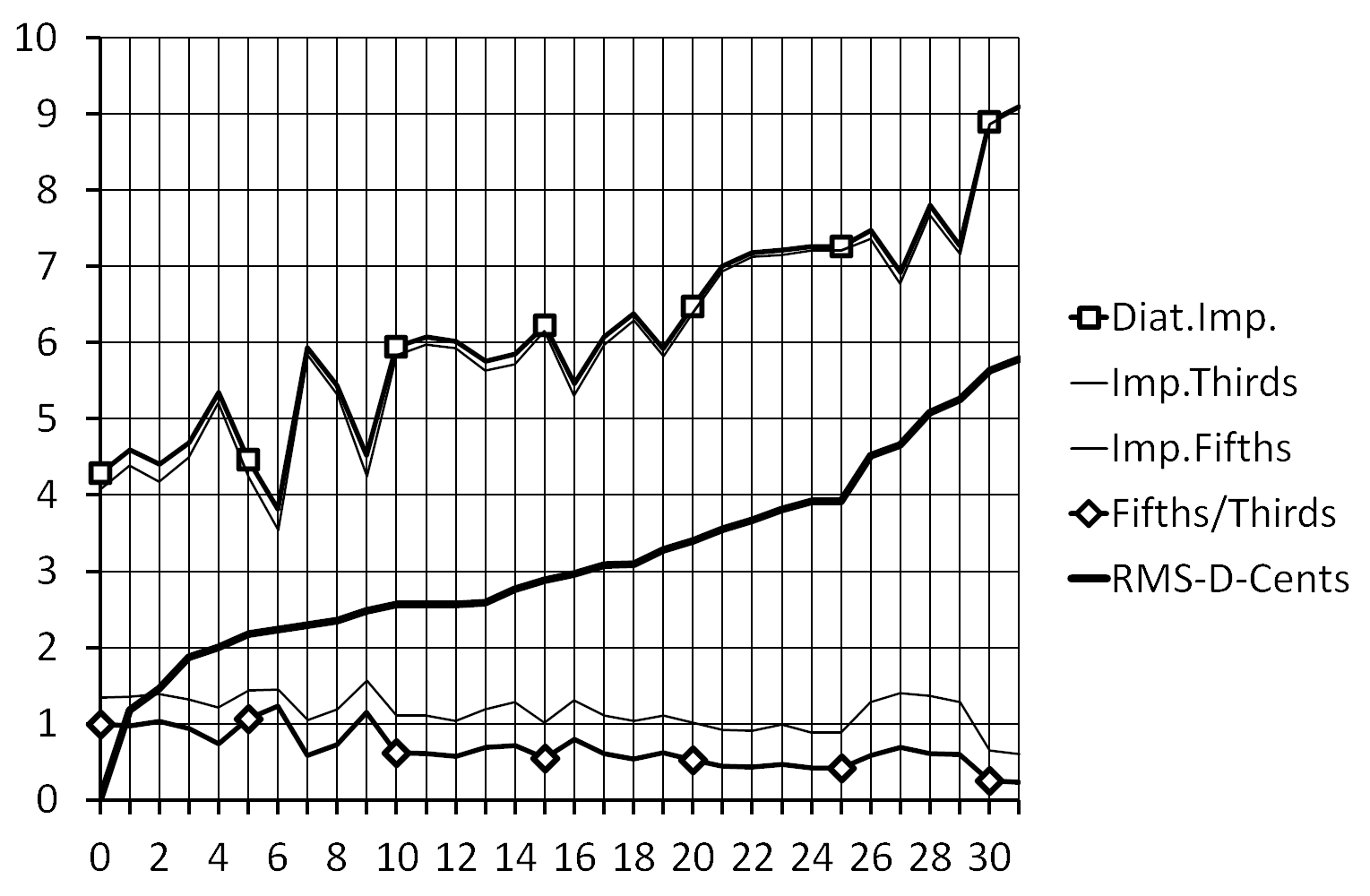
Figure 9: Historical WT characteristics ranked according table 9

Notice the low diatonic C-major impurity at position 6 (Vogel).
The C-major diatonic impurity is only slightly higher than the thirds impurity. It should be noticed here that many publications duly attach much attention indeed to major thirds quality. But it is striking on the other hand, that the Beat-WT model is determined by the weights of minor thirds only ($P_{MT}=0$; $P_{mt}=0.1177$; tables 6, 7). Best mathematical fit with historical temperaments also, is obtained with similar weights criteria; ($P_{MT}=0$; $P_{mt}=0.07$) for the collection of (K/N) marked WT, and ($P_{MT}=0$; $P_{mt}=0.0053$) for the full WT collection; all with $P_{MT}=0$.
The weighted Fifths/Thirds impurity ratios of the best ranked historical WT have values close to -1- (one), the ratio chosen for elaboration of the Beat-WT model. The fifths impurities show a slow and minor decrease, and have an almost parallel course with the weighted Fifths/Thirds impurity ratio.
The already mentioned downwards shift of Neidhardt and Werckmeister in table 9 is probably due to observable small deviations of thirds characteristics, see fig. 11 and 11; probably also for Billeter, not here displayed. A remarkable symmetry can be observed, and the symmetry is perfect for the Beat-WT model. Symmetry is discussed in more detail in appendix B.2.

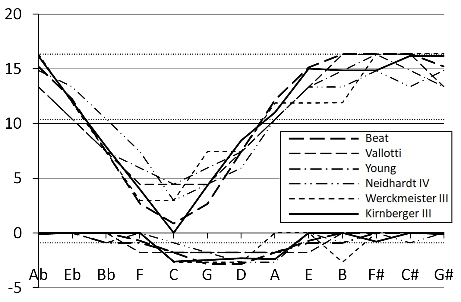
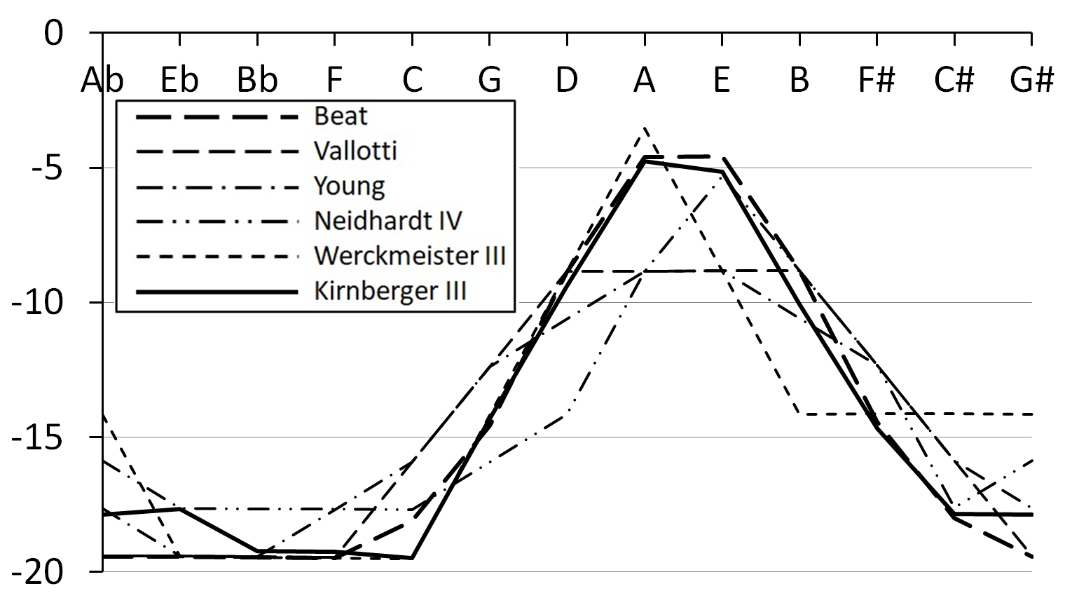
Figure 10: Beat impurity of major thirds (up) and fifths (down)

Figure 11: Beat impurity of minor thirds

4 Course of Diatonic Impurity, versus Tonality

The C-major optimisation raises the question of what happens to other tonalities. It is to be expected that the unweighted diatonic impurity will increase with remote tonalities. Other question is how this stands comparing temperament families.

Table 10 displays the numerical courses of the diatonic impurities of the 12TET, the meantone, Kirnberger III, and the unexplored EF-Beat-WT (§ 2.2.1.3; Appendix A.3 table 11). Major tonalities that are admitted in meantone are displayed in the upper part of the table.

Admitted Tonalities	B$\flat$	F	C	G	D	A
12TET	9.30	9.30	9.30	9.30	9.30	9.30
Meantone	3.18	3.18	3.18	3.18	3.18	3.18
Kirnberger III	8.50	5.86	4.81	6.11	8.33	10.38
EF-Beat-WT	8.96	5.31	3.18	5.31	8.97	11.71
Remote Ronalities	E	B	F$\sharp$	C$\sharp$ / D$\flat$	Ab	E$\flat$
12TET	9.30	9.30	9.30	9.30	9.30	9.30
Meantone	15.48	21.19	25.65	25.65	21.19	15.48
Kirnberger III	11.63	12.43	12.69	12.98	12.44	10.86
EF-Beat-WT	13.09	13.38	13.55	13.38	13.09	11.71

Table 10: Diatonic Beat Impurity of Tonalities

The meantone has remarkable characteristics, and is of special interest still, for specific Baroque music: especially fig. 12 dramatically illustrates the meantone characteristics course.

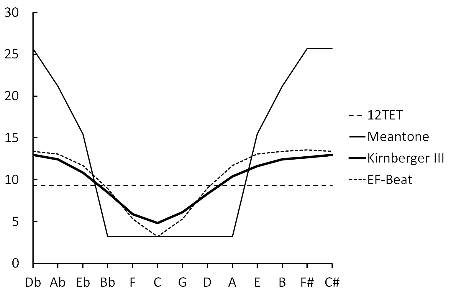
Figure 12: Diatonic Impurity of Tonalities

• Surprisingly equal and excellent quality for all admitted tonalities, offering good modulations in a limited range of tonalities. Mozart, for example, usually stays within this domain (about 85% of his corpus), exceptionally using the E or E$\flat$ key, but never as far as the B key (Kelletat, 1982, p. 11).

• Excessive impurity, up to dissonance, for the remote tonalities.

• Specific meantone characteristics are sometimes deliberately exploited. A typical example consists of certain dramatic and highly dissonant passages of J. S. Bach’s “St. Matthew Passion”; for instance: proposal for crucifixion, death of Jesus, and a number of other outstanding dramatic events, …(Kelletat, 1982, p. 20). Kelletat also cites Händel within this context, and many other examples can certainly be given by music connoisseurs and historians.

It is not always obvious to choose between meantone or a WT. Possibilities for an artistic choice will remain, even within one family. A WT can be chosen among typical ones like those displayed in fig. 11, 11, and 13, or some with a flatter course like those below Werckmeister III in the ranking table 8 or 9, or down to the perfectly flat 12TET as an extreme.

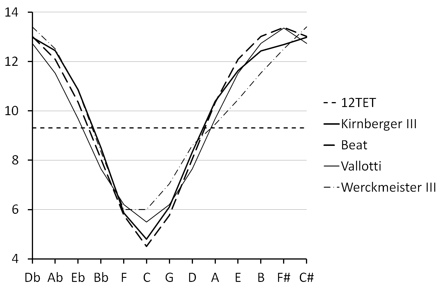
Figure 13: Diatonic Impurity of WT Tonalities

5 Conclusions

A number of models with ultimate diatonic C-major purity were developed.
Those models, were used for a proposed objective ranking of historical WT temperaments. Widely prevailing musical appreciations of historical WT temperaments, and their obtained objective mathematical ranking, are in good agreement.
There is always a close fit of some selected better models with a famous and recognised historical temperament. Kirnberger III is always on top of the rankings, Werckmeister III is probably acceptable as a limit for recommendable WT.

Werckmeister’s / Kelletat’s musical WT definition

has gained an analysed mathematical support

The list of WT temperaments is very well filled, in small steps, starting at the models on top, down to the lower WT limit; -the 12TET temperament-.

The development of new WT achieves very little

Because of artistic criteria, a need for choice of WT temperament persists.

Even a need to leave the WT domain persists, and will not vanish.

Supplemental online material

Supplemental online material for this article can be accessed at doi-provided-by-publisher. It offers all calculations and solutions discussed in this paper, on a spreadsheet, and allows for observation of the behavior of musical intervals, in dependence of the entered weighting parameters.

Disclosure statement

No potential conflict of interest was reported by the author.

6   Formulas

6.1 Formulas for § 2.2.1 First Model

With: A=440

$\frac{\partial}{\partial C}\mathrm{:}\quad(25P_{MT}P_{C}^{2}+100P_{mt}P_{A}^{2}+9P_{C}^{2}+16P_{F}^{2})C-20P_{MT}P_{C}^{2}E-12P_{F}^{2}F-6P_{C}^{2}G$

$=60P_{mt}P_{A}^{2}A$

$\frac{\partial}{\partial D}\mathrm{:}\quad(36P_{mt}P_{D}^{2}+100P_{mt}P_{B}^{2}+9P_{D}^{2}+16P_{G}^{2})D-30P_{mt}P_{D}^{2}F-12P_{G}^{2}G-60P_{mt}P_{B}^{2}B$

$=6P_{D}^{2}A$

$\frac{\partial}{\partial E}\mathrm{:}\quad-20P_{MT}P_{C}^{2}C+(16P_{MT}P_{C}^{2}+36P_{mt}P_{F}^{2}+9P_{E}^{2}+16P_{A}^{2})E-30P_{mt}P_{E}^{2}G-6P_{E}^{2}B$

$=12P_{A}^{2}A$

$\frac{\partial}{\partial F}\mathrm{:}\quad-12P_{F}^{2}C-30P_{mt}P_{D}^{2}D+(25P_{MT}P_{F}^{2}+25P_{mt}P_{D}^{2}+9P_{F}^{2})F=20P_{MT}P_{E}^{2}A$

$\frac{\partial}{\partial G}\mathrm{:}\quad-6P_{C}^{2}C-12P_{G}^{2}D-30P_{mt}P_{E}^{2}E+(25P_{MT}P_{G}^{2}+25P_{mt}P_{E}^{2}+4P_{C}^{2}+9P_{G}^{2})G$

$-20P_{MT}P_{G}^{2}B=0$

$\frac{\partial}{\partial B}\mathrm{:}\quad-60P_{mt}P_{B}^{2}D-6P_{E}^{2}E-20P_{MT}P_{G}^{2}G+(16P_{MT}P_{G}^{2}+36P_{mt}P_{B}^{2}+4P_{E}^{2})B=0$

The obtained $B$ and $F$ values have to be entered in equations concerning altered notes.

$\frac{\partial}{\partial C\sharp}\mathrm{:}\quad(9P_{C\sharp}^{2}+16P_{F\sharp}^{2})C\sharp-12P_{F\sharp}^{2}F\sharp-6P_{C\sharp}^{2}G\sharp=0$

$\frac{\partial}{\partial F\sharp}\mathrm{:}\quad-12P_{F\sharp}^{2}C\sharp+(9P_{F\sharp}^{2}+16P_{B}^{2})F\sharp=12P_{B}^{2}B$

$\frac{\partial}{\partial G\sharp}\mathrm{:}\quad-6P_{C\sharp}^{2}C\sharp+(4P_{C\sharp}^{2}+9P_{G\sharp}^{2})G\sharp-12P_{G\sharp}^{2}E\flat=0$

$\frac{\partial}{\partial E\flat}\mathrm{:}\quad-12P_{G\sharp}^{2}G\sharp+(16P_{G\sharp}^{2}+9P_{E\flat}^{2})E\flat-6P_{Eb}^{2}B\flat=0$

$\frac{\partial}{\partial B\flat}\mathrm{:}\quad-6P_{E\flat}^{2}E\flat+(4P_{E\flat}^{2}+9P_{B\flat}^{2})B\flat=12P_{B\flat}^{2}F$

6.2 Formulas for § 2.2.2 Domain for $B=kF$, with $k=2^{10}/3^{6}$

With: A=440 and $k=2^{10}/3^{6}$

$\frac{\partial}{\partial C}\mathrm{:}\quad(25P_{C}^{2}P_{MT}+100P_{A}^{2}P_{mt}+9P_{C}^{2}+16P_{F}^{2})C-20P_{C}^{2}P_{MT}E-12P_{F}^{2}F-6P_{C}^{2}G$

$=60P_{A}^{2}P_{mt}A$

$\frac{\partial}{\partial D}\mathrm{:}\quad(36P_{D}^{2}P_{mt}+100P_{B}^{2}P_{mt}+9P_{D}^{2}+16P_{G}^{2})D-(30P_{D}^{2}P_{mt}+60kP_{B}^{2}P_{mt})F-12P_{G}^{2}G$

$=6P_{D}^{2}A$

$\frac{\partial}{\partial E}\mathrm{:}\quad-20P_{C}^{2}P_{MT}C+(16P_{C}^{2}P_{MT}+36P_{E}^{2}P_{mt}+9P_{E}^{2}+16P_{A}^{2})E-6kP_{E}^{2}F-30P_{E}^{2}P_{mt}G$

$=12P_{A}^{2}A$

$\frac{\partial}{\partial F}\mathrm{:}\quad+(25P_{F}^{2}P_{MT}+16k^{2}P_{G}^{2}P_{MT}+25P_{D}^{2}P_{mt}+36k^{2}P_{B}^{2}P_{mt}+4k^{2}P_{E}^{2}+9P_{F}^{2})F-12P_{F}^{2}C$

$-(30P_{D}^{2}P_{mt}+60kP_{B}^{2}P_{mt})D-6kP_{E}^{2}E-20kP_{G}^{2}P_{MT}G=20P_{F}^{2}P_{MT}A$

$\frac{\partial}{\partial G}\mathrm{:}\quad-6P_{C}^{2}C-12P_{G}^{2}D-30P_{E}^{2}P_{mt}E-20kP_{G}^{2}P_{MT}F$

$+(25P_{G}^{2}P_{MT}+25P_{E}^{2}P_{mt}+4P_{C}^{2}+9P_{G}^{2})G=0$

6.3 Solution for § 2.2.1.3  Domain above the AB line, fig. 5

The model of § 2.2.1, for $P_{MT}=P_{mt}=1$, has major thirds on E, B, F$\sharp$, C$\sharp$ and G$\sharp$ exceeding the 81/64 ratio, and major thirds on F, C and G below the 5/4 ratio. This goes against the formula 2 conditions. Compliance with those conditions was achieved in § 2.2.2, by presetting the AB-line condition (see § 2.2.1.1, setting B=kF, and fig. 5).

An alternate way to achieve compliance with formula 2, might be, in a first step, to preset an 81/64 ratio for thirds standing on the diatonic major thirds (e.g. E-G$\sharp$ and G$\sharp$-C, on C-E), see fig. A1. This involves all above mentioned major thirds, except the one on F$\sharp$.

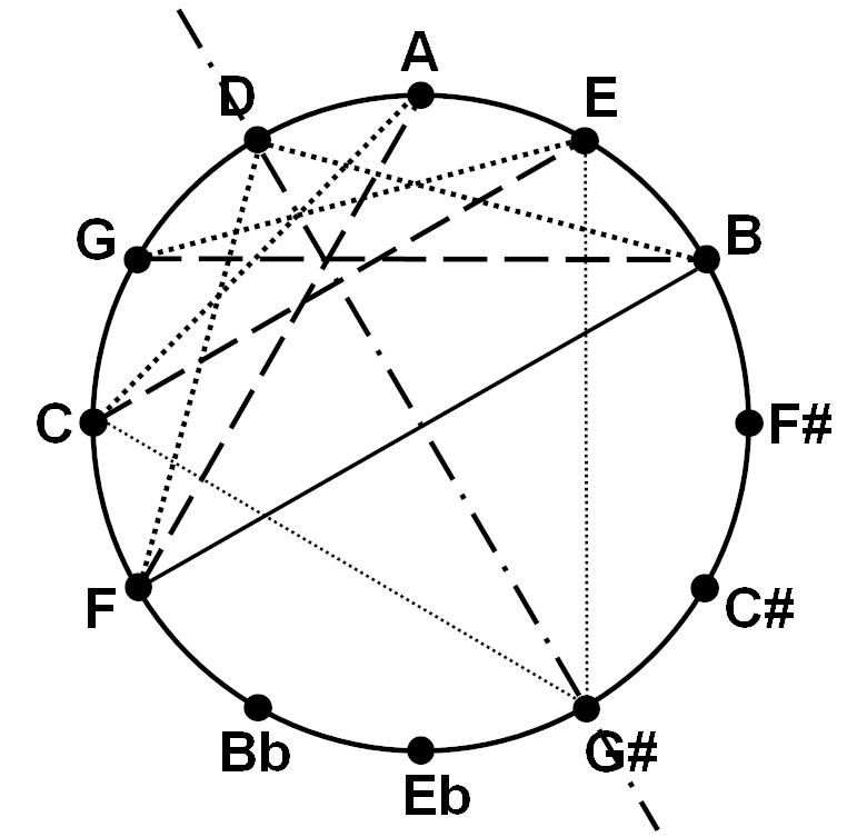
Figure 14: Important Diatonic Intervals

The obtained models have up to seven major thirds with the 81/64 ratio, but none exceeds this ratio; the major thirds on F, C and G have a ratio $m=3^{8}/2^{13}$, still below the 5/4 ratio; the models are therefore, still not complying. The model interval courses are similar to those displayed in fig. A2. Those courses reveal that the required just major thirds on F, C and G can be obtained, by a suitable adaptation of involved thirds:

• Maintain a pythagorean major third on B and C$\sharp$, with a just third on F and G; this also leads to complying fixed 512/405 ratio thirds on E$\flat$ and A

• The just third on C: leave the thirds on E and G$\sharp$ unknown (hence: G$\sharp$=variable);

With m=4/5, the above leads to following substitutions in formulas 13 and 14:

$F=mA$; $C=mE$; $G=mB$;$\quad C\#={\frac{64}{81}}F$; $Eb={\frac{81}{128}}B$

Partial derivatives for some notes expire, and so do the expressions for fixed major thirds. The remaining partial derivatives of formulas 13 and 14, set to zero, lead to:

$\frac{\partial}{\partial D}\mathrm{:}\quad(36P_{D}^{2}P_{mt}+100P_{B}^{2}P_{mt}+9P_{D}^{2}+16P_{G}^{2})D-(60P_{B}^{2}P_{mt}+12mP_{G}^{2})B$

$=(30mP_{D}^{2}P_{mt}+6P_{D}^{2})A$

$\frac{\partial}{\partial E}\mathrm{:}\quad(36P_{E}^{2}P_{mt}+100m^{2}P_{A}^{2}P_{mt}+9m^{2}P_{C}^{2}+9P_{E}^{2}+16m^{2}P_{F}^{2}+16P_{A}^{2})E$

$-(30mP_{E}^{2}P_{mt}+6m^{2}P_{C}^{2}+6P_{E}^{2})B=(60mP_{A}^{2}P_{mt}+12m^{2}P_{F}^{2}+12P_{A}^{2})A$

$\frac{\partial}{\partial B}\mathrm{:}\quad-(60P_{B}^{2}P_{mt}+12mP_{G}^{2})D-(30mP_{E}^{2}P_{mt}+6m^{2}P_{C}^{2}+6P_{E}^{2})E$

$+(25m^{2}P_{E}^{2}P_{mt}+36P_{B}^{2}P_{mt}+4m^{2}P_{C}^{2}+4P_{E}^{2}+9m^{2}P_{G}^{2})B=0$

Only F$\sharp$, G$\sharp$ and B$\flat$ remain to be solved, based on the obtained B and F values.

$\frac{\partial}{\partial F\sharp}\mathrm{:}\quad(16P_{B}^{2}+9P_{F\sharp}^{2})F\sharp={\frac{256}{27}}P_{F\sharp}^{2}F+12P_{B}^{2}B$

$\frac{\partial}{\partial G\sharp}\mathrm{:}\quad(4P_{C\sharp}^{2}+9P_{G\sharp}^{2})G\sharp=\frac{243}{32}P_{C\sharp}^{2}F+\frac{243}{32}P_{G\sharp}^{2}B$

$\frac{\partial}{\partial B\flat}\mathrm{:}\quad(4P_{E\flat}^{2}+9P_{B\flat}^{2})B\flat=12P_{B\flat}^{2}F+{\frac{243}{64}}P_{E\flat}^{2}B$

The above conditions, combined with the condition of balanced thirds and fifths (see § 2.2.2; formula 17, and fig. 9), lead with (PMT=0; Pmt=.33287) to the model holding pitches displayed in table A1:

EF-Beat-WT	C	C$\sharp$	D	E$\flat$	E	F
Pitches	263.32	278.12	294.40	311.64	329.15	352.00
EF-Beat-WT	F$\sharp$	G	G$\sharp$	A	B$\flat$	B
Pitches	370,09	393.97	416.35	440.00	468.39	492.47

Table 11: EF-Beat-WT model   (*) EF: Enlarged Fifth

Fig. 15 displays the interval characteristics of this model, also in comparison of those of Vogel (see also § 3.1.1, table 8, and comments). This model’s unweighted diatonic purity is better than Vogel’s one: 3.184 against 3.997.

Musical differences with historical WT are prominent (see fig. 15).

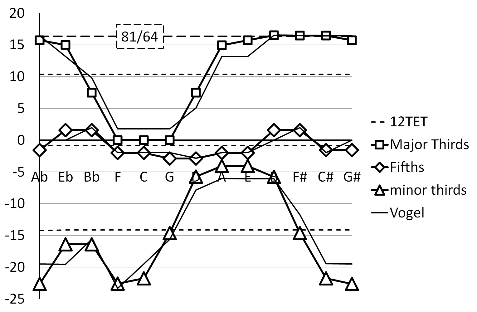
Figure 15: Ultimate WT: EF-Beat-WT

• Pythagorean major thirds: This model contains seven major thirds, very close or equal to the 81/64 Pythagorean ratio.

• Fifths containing an altered note: four of those fifths are enlarged and grouped in a specific way, allowing persistent fifths enlargement, without inducing major thirds to exceed the 81/64 Pythagorean ratio.

This model and Vogel are part of a possible but yet unexplored musical WT domain.

Musical practice based on this model might be topic of musical experimentation, this falls however outside the scope of this paper.

7   Application of Interval RATIO Measurements

7.1 Relation between interval ratio, and interval impurity measurement

Interval ratio impurity measurements, like PBP, PPD or Cent (formula 7-9), allow for simplifications.

$$\mathrm{Let\quad}\frac{x_{2}}{x_{1}}\mathrm{,}\frac{x_{3}}{x_{2}}\mathrm{,\dots,}\frac{x_{n}}{x_{n-1}}\mathrm{,\dots,}\frac{kx_{1}}{x_{p}}\mathrm{\quad for\quad n=1\ to\ p;\ and\quad k=\quad a\ fixed\ value}\\$$ (19)

be a series of intervals (ratios), wherefore the expression below should be minimised.

$$F_{x}(x_{1}\mathrm{,\dots}x_{n}\mathrm{,\dots}x_{p})=\left[F_{a}\left(\frac{x_{2}}{x_{1}}\right)\right]^{2}+\left[F_{a}\left(\frac{x_{3}}{x_{2}}\right)\right]^{2}\mathrm{\dots}+\left[F_{a}\left(\frac{x_{n}}{x_{n-1}}\right)\right]^{2}\mathrm{\dots}+\left[F_{a}\left(\frac{kx_{1}}{x_{p}}\right)\right]^{2}$$ (20)

Setting the partial derivatives to zero, this is $\frac{\partial F_{x}}{\partial x_{n}}=0$ for $n=1$ to $p$, leads to

$$F_{a}\left(\frac{x_{n}}{x_{n-1}}\right)=F_{a}\left(\frac{x_{n+1}}{x_{n}}\right)\mathrm{\quad for\ }n=2\mathrm{\quad to\quad}(p-1)\mathrm{\quad but\ also\quad}$$ (21)

$$F_{a}\left(\frac{x_{2}}{x_{1}}\right)=F_{a}\left(\frac{kx_{1}}{x_{p}}\right)\mathrm{\quad for\ }n=1\mathrm{\quad and\quad}F_{a}\left(\frac{x_{p}}{x_{p-1}}\right)=F_{a}\left(\frac{kx_{1}}{x_{p}}\right)\mathrm{\quad for\ }n=p$$ (22)

Hence, all functions $F_{a}\left(\frac{x_{n+1}}{x_{n}}\right)$ for $n=1$ to $(p-1)$, and $F_{a}\left(\frac{kx_{1}}{x_{p}}\right)$ must have equal value.

A possible solution, not excluding any other one, therefore contains the equalities

$$\frac{x_{2}}{x_{1}}=\frac{x_{3}}{x_{2}}=\mathrm{,\dots,}=\frac{x_{n}}{x_{n-1}}=\mathrm{,\dots,}\frac{x_{p}}{x_{p-1}}=\frac{kx_{1}}{x_{p}}=C_{t}\\$$ (23)

Conclusion:
For a group composed of equal type intervals, the best group quality is obtained at equality of ratio of all intervals, if the impurity measurement is based on measuring the ratios of the note pitches of the intervals.

7.2 Models Symmetry

Examination of optimised Beat models revealed remarkable symmetrical characteristics, see fig. 11, 12, and fig. 15. Further examination of the circle of fifths fig. 14 reveals furthermore:

• A symmetric geometric structure can be observed on the circle of fifths, for intervals concerned in the calculation of the diatonic impurity: fig. 14 depicts fifths as thirty degree arcs on the circle, thirds as arc cords, drawn as striped lines (major thirds) or dotted lines (minor thirds).
  A symmetry axis passes by the notes D and G$\sharp$.
  Notice: on the keyboard too, D and G$\sharp$ are (optical) symmetry centers

• Because of, and thanks to this symmetry and ratio measuring units, we have :

  1. equality of diatonic fifths F-C and E-B; C-G and A-E; G-D and D-A

  2. equality of diatonic major thirds F-A and G-B

  3. equality of diatonic minor thirds D-F and B-D; A-C and E-G

  4. equality of fifths with altered notes: B-F$\sharp$ and B$\flat$-F; F$\sharp$-C$\sharp$ and E$\flat$-B$\flat$; C$\sharp$-G$\sharp$ and G$\sharp$-E$\flat$ ($\div$A$\flat$-E$\flat$)

  5. D and G$\sharp$ are exactly diametrically opposite

  6. a reduction of the number of variable notes: reduction to three for the C-major diatonic notes, and two for the altered notes.
     The chosen notes have to be paired and independent, we therefore have:

     • For the C-major diatonic notes: F (or B), C (or E) and D

     • For the altered notes: C$\sharp$ (or E$\flat$) and F$\sharp$ (or B$\flat$); (G$\sharp$ depends on D: point 5)

7.2.1 Substitutions / possible eliminations

Some notes can be substituted, in line with the observations at Section B.2.

$$\mathrm{}\mathrm{Notes\ C\ or\ E:\quad we\ have\quad}\frac{E}{D}=\frac{D}{C}\mathrm{\quad hence\quad}C=\frac{D^{2}}{E}$$ (24)

$$\mathrm{}\mathrm{Note\ G:\quad we\ have,\ counting\ the\ octaves\quad}\frac{A}{D}=\frac{2D}{G}\mathrm{\quad hence\quad}G=\frac{2D^{2}}{AE}$$ (25)

Notes F or B; we have, counting the octaves

$$\frac{B}{D}=\frac{2D}{F}\qquad\mathrm{\ hence}\qquad F=\frac{2D^{2}}{B}$$ (26)

Notes D and G$\sharp$ being diametrically opposite, we have

$$\qquad G\sharp=D\sqrt{2}$$ (27)

Possible additional substitution (for models with $B/F=2^{10}/3^{6}$)

Six perfect fifths between B to F, containing an altered note, means also three perfect fifths from G$\sharp$ to F. Setting F and B to the same octave, it can be said.

$$B=\frac{2^{10}}{3^{6}}F\mathrm{\quad and\quad}F=\frac{3^{3}}{2^{5}}G\sharp=\frac{3^{3}}{2^{5}}\sqrt{2}D\mathrm{\quad hence\quad}B=\frac{2^{5.5}}{3^{3}}D$$ (28)

Possible additional elimination (for WT models with $B/F=2^{10}/3^{6}$)

See fig. 14. The line connecting F to B stands perpendicular to the G$\sharp$-D diameter and has a fixed value, because $B/F=2^{10}/3^{6}$; the lines F-D and D-B therefore have a fixed value too. In other words: the minor thirds B-D et D-F have a fixed value, totally independent of the $P_{MT}$ and $P_{mt}$ weighing parameters; their ratio equals $2^{5}/3^{3}=1.185…$
The expressions representing those minor thirds impurity may consequently be eliminated in the sum of squares, formula 13, while, being constants, their partial derivatives will be zero.

7.2.2 Model calculation with Cents (for WT models with $B/F=2^{10}/3^{6}$)

Impurity formulas: expressions for minor thirds impurities on notes D and B can be eliminated (see § B.2.1.2).

Major thirds impurities:	Fifths impurities
C: $\Delta MT_{C}=1200\log{(4E/5C)}/\log{2}$	C: $\Delta Fi_{C}=1200\log{(2G/3C)}/\log{2}$
F: $\Delta MT_{F}=1200\log{(4A/5F)}/\log{2}$	D: $\Delta Fi_{D}=1200\log{(2A/3D)}/\log{2}$
G: $\Delta MT_{G}=1200\log{(4B/5G)}/\log{2}$	E: $\Delta Fi_{E}=1200\log{(2B/3E)}/\log{2}$
minor thirds impurities:	F: $\Delta Fi_{F}=1200\log{(4C/3F)}/\log{2}$
D: eliminated	G: $\Delta Fi_{G}=1200\log{(4D/3G)}/\log{2}$
E: $\Delta mt_{E}=1200\log{(5G/6E)}/\log{2}$	A: $\Delta Fi_{A}=1200\log{(4E/3A)}/\log{2}$
A: $\Delta mt_{A}=1200\log{(10C/6A)}/\log{2}$	B: A diatonic fifth on B does not exist:
B: eliminated	a perfect fifth on B leads indeed to F#

Table 12: Diatonic C-major impurities

The notes F, C, G, and B can be substituted: formulas (24; 25; 26; 28).
With $k=3^{3}/2^{4,5}$ the sum of squares of impurities becomes

$$P_{MT}\left\{\left[\log{\left(\frac{4E^{2}}{5D^{2}}\right)}\right]^{2}+2\left[\log{\left(\frac{4A}{5kD}\right)}\right]^{2}\right\}+2P_{mt}\left[\log{\left(\frac{5D^{2}}{3AE}\right)}\right]^{2}$$

$$+2\left\{\left[\log{\left(\frac{4E}{3A}\right)}\right]^{2}+\left[\log{\left(\frac{2A}{3D}\right)}\right]^{2}+\left[\log{\left(\frac{4D}{3kE}\right)}\right]^{2}\right\}$$ (29)

The partial derivatives of remaining variables D and E, set to zero, lead to

$\frac{\partial}{\partial D}\mathrm{:}\quad(3P_{MT}+4P_{mt}+2)\log{D}-(2P_{MT}+2P_{mt}+1)\log{E}$

$=(4P_{MT}-1)\log 2+2P_{mt}\log 3-2(P_{MT}+P_{mt})\log 5-(P_{MT}-1)\log{k}$

$$+(P_{MT}+2P_{mt}+1)\log{A}\qquad\qquad\qquad\qquad\qquad\qquad\qquad\qquad$$ (30)

$\frac{\partial}{\partial E}\mathrm{:}\quad-(2P_{MT}+2P_{mt}+1)\log{D}+(2P_{MT}+P_{mt}+2)\log{E}$

$$=-2P_{MT}\log 2-P_{mt}\log 3+(P_{MT}+P_{mt})\log 5-P_{Fi}\log{k}-(P_{MT}-1)\log{A}$$ (31)

The solution can be calculated in a spreadsheet that can be downloaded.
Pitches of Kirnberger III, and those obtained here for this Cent-WT model with balanced impurity of thirds and fifths (applying formula 17, see also fig. 9), and those of the Beat-WT model § 2.2.2, table 7, are very similar (see table 13):

	C	C$\sharp$	D	E$\flat$	E	F
Cent-WT	263.24	277.56	294.40	312.26	329.26	351.29
Beat-WT	263.23	277.55	294.39	312.25	329.25	351.28
Kirnberger III	263.20	277.32	294.20	311.94	329.00	350.93
	F$\sharp$	G	G$\sharp$	A	B$\flat$	B
Cent-WT	370.08	393.96	416.35	440.00	468.39	493.45
Beat-WT	370.07	393.95	416.33	440.00	468.37	493.43
Kirnberger III	370,13	393.50	415.98	440.00	467.91	493.50

Table 13: Comparison of Kirnberger III, and optimal Cent and Beat models

7.3 Kirnberger III

A preset of a just major third on C, taking into account all preceding considerations of this appendix, allows for following additional substitution of E in proportion to D, so that only one variable remains: the note D:

$$E=\frac{5C}{4}\quad\mathrm{but}\quad C=\frac{D^{2}}{E}\quad\mathrm{(form.\ \ref{equ B6});\ hence}\quad E=\frac{\sqrt{5}}{2}D$$

7.3.1 Cent Model

The derivative by D, of the sum of squares, set to zero (with $k=3^{3}/2^{4.5}$), leads to

$$\log{D}=\log{A}+\frac{P_{MT}\log{(\frac{4}{5k})}-P_{mt}\log{(\frac{2\sqrt{5}}{3})}-\log{(\frac{2\sqrt{5}}{3})}+\log{(\frac{2}{3})}}{P_{MT}+P_{mt}+2}$$

Model with balanced thirds/fifths: $RMS$-$\Delta$-$Cent=1.18$ if compared to Kirnberger III.

7.3.2 Beat Model

Based on the same symmetry considerations as for the ratio based Cent and PBP models, a Beat model (Beat / PBP equivalence: see § 1.4.2) can be solved . The outcome (with $k=3^{3}/2^{4.5}$) leads to

$$D=\frac{20kP_{MT}P_{F}^{2}+\frac{120P_{mt}P_{A}^{2}}{\sqrt{5}}+6\sqrt{5}P_{A}^{2}+6P_{D}^{2}}{25kP_{MT}P_{F}^{2}+80P_{mt}P_{A}^{2}+20P_{A}^{2}+9P_{D}^{2}}A$$

Model with balanced thirds/fifths: $RMS$-$\Delta$-$Cent=1.18$ if compared to Kirnberger III.
This model is almost identical to the above Cent model, § B.3.1 .

7.3.3 Optimisation of fifths only (Cent and Beat)

With $P_{MT}=P_{mt}=0$ the outcome is:

• Fifths on C, G, D, A: $ratio=5^{(1/4)}$

• Fifths on B, F$\sharp$, C$\sharp$, G$\sharp$, E$\flat$, B$\flat$: $ratio=3/2$

• Fifths on F, E: $ratio=(2^{6}/3^{3})(2/5)^{(1/2)}$

Model comparison: $RMS$-$\Delta$-$Cent=0.945$ if compared to Kirnberger III.

Fig 01.jpg: (fig. 1) Orgelprobe 1681
Fig 02.jpg: (fig. 2) C-major diatonic structure
Fig 03.jpg: (fig. 3) Beating of a musical interval
Fig 04.jpg: (fig. 4) Impact of squares
Fig 05.jpg: (fig. 5) Diatonic Impurity as $F(P_{MT}$; $P_{mt}$)
Fig 06.jpg: (fig. A1) Important Diatonic Intervals
Fig 07 new.jpg: (fig. 6) Diatonic Impurity as $F(P_{MT}$; $P_{mt}$)
Fig 08.jpg: (fig. 7) Course of unweighted diatonic thirds and fifths
Fig 09.jpg: (fig. 8) Course of weighted diatonic thirds and fifths
Fig 10.jpg: (fig. 9) Historical WT characteristics ranked according table 9
Fig 11.jpg: (fig. 10) Beat impurity of major thirds (up) and fifths (down)
Fig 12.jpg: (fig. 11) Beat impurity of minor thirds
Fig 13.jpg: (fig. 12) Diatonic Impurity of Tonalities
Fig 14.jpg: (fig. 13) Diatonic Impurity of WT Tonalities
Fig 15.jpg: (fig. A2) Ultimate WT: EF-Beat-WT

Table 01: Note weights applicable with Beat impurity measurements
Table 02: Diatonic C-major impurities
Table 03: Impurities of fifths containing an altered note
Table 04: Weighted Diatonic Impurity
Table 05: Beat-WT-A and Beat-WT-B
Table 06: Impurities of Fifths and the C-major diatonic scale
Table 07: impurity = 2.7024; (4.2928 unweighted) Beat-WT $P_{MT}=0$; $P_{mt}=0.1177$
Table 08: WT Diatonic C-major Impurities
Table 09: $RMS$-$\Delta$-$Cents$ comparison of historical WT temperaments with Beat model
Table 10: Diatonic Beat Impurity of Tonalities

Table A1: EF-Beat-WT model (*) EF: Enlarged Fifth

Table B1: Diatonic C-major impurities
Table B2: Comparison of Kirnberger III, and optimal Cent and Beat models

References

- Amiot (2009) Amiot E. 2009: “Discrete Fourier Transform and Bach’s Good Temperament”. Society for Music Theory; Music Theory Online, Volume 15, Number 2, June 2009.
- Amiot (2010) Amiot E. 2010: “Modèles algébriques et algorithmes pour la formalisation mathématique de structures musicales” Université Pierre et Marie Curie