Gapped vegetation patterns: crown/root allometry and snaking bifurcation

Abstract

Nonuniform spatial distributions of vegetation in scarce environments consist of either gaps, bands often called tiger bush or patches that can be either self-organized or spatially localized in space. When the level of aridity is increased, the uniform vegetation cover develops localized regions of lower biomass. These spatial structures are generically called vegetation gaps. They are embedded in a uniform vegetation cover. The spatial distribution of vegetation gaps can be either periodic or randomly distributed. We investigate the combined influence of the facilitative and the competitive nonlocal interactions between plants, and the role of crow/root allometry, on the formation of gapped vegetation patterns. We characterize first the formation of the periodic distribution of gaps by drawing their bifurcation diagram. We then characterize localized and aperiodic distributions of vegetation gaps in terms of their snaking bifurcation diagram.

1 Introduction

When the level of the aridity increases, vegetation populations exhibit two-phase structures where high biomass areas are separated by sparsely covered or even bare ground. The spatial fragmentation of landscapes leading to the formation of vegetation patterns in semi- and arid-ecosystems is attributed to the symmetry-breaking instability that occurs even under strictly homogeneous and isotropic environmental conditions [1]. On-site measurements supported by theoretical modeling showed indeed that vegetation patterns are formed thanks to the facilitation and competition plant-to-plant interactions [2, 3, 4, 5]. The periodic vegetation patterns that emerge at the onset of this instability are characterized by a well-defined wavelength. Generally speaking, symmetry-breaking instability requires two opposite feedbacks that act on different spatial scales. The positive feedback consists of the facilitative plant-to-plant interaction such as shadow and shelter effect. This feedback operates on a small spatial scale comparable to the size of the plant crown and tends to improve the water budget in the soil [6], which thus favors the increase of vegetation biomass in arid-zones. The negative feedback by competitive plant-to-plant interaction for resources such as water and nutrients which on the contrary operates on a longer space scale corresponding to the plant lateral root length. The roots of a given plant tend to deprive its neighbors’ resources such as water [7]. The balance of competition and facilitation interactions within plant communities allow for the stabilization of vegetation patterns. This symmetry-breaking instability is characterized by an intrinsic wavelength that is solely determined by dynamical parameters such as the structural parameter (the ratio between the size of the crown and the rhizosphere) and the vegetation community cooperatively parameter or other internal effects [8, 9]. The morphologies of these states follow the generic sequence gaps $\iff$ bands or labyrinth $\iff$ spots as the level of the aridity is increased [10, 11]. This generic scenario has been recovered for other mathematical models that incorporate water transport by below ground and/or above ground run-off [12, 13, 14, 15].

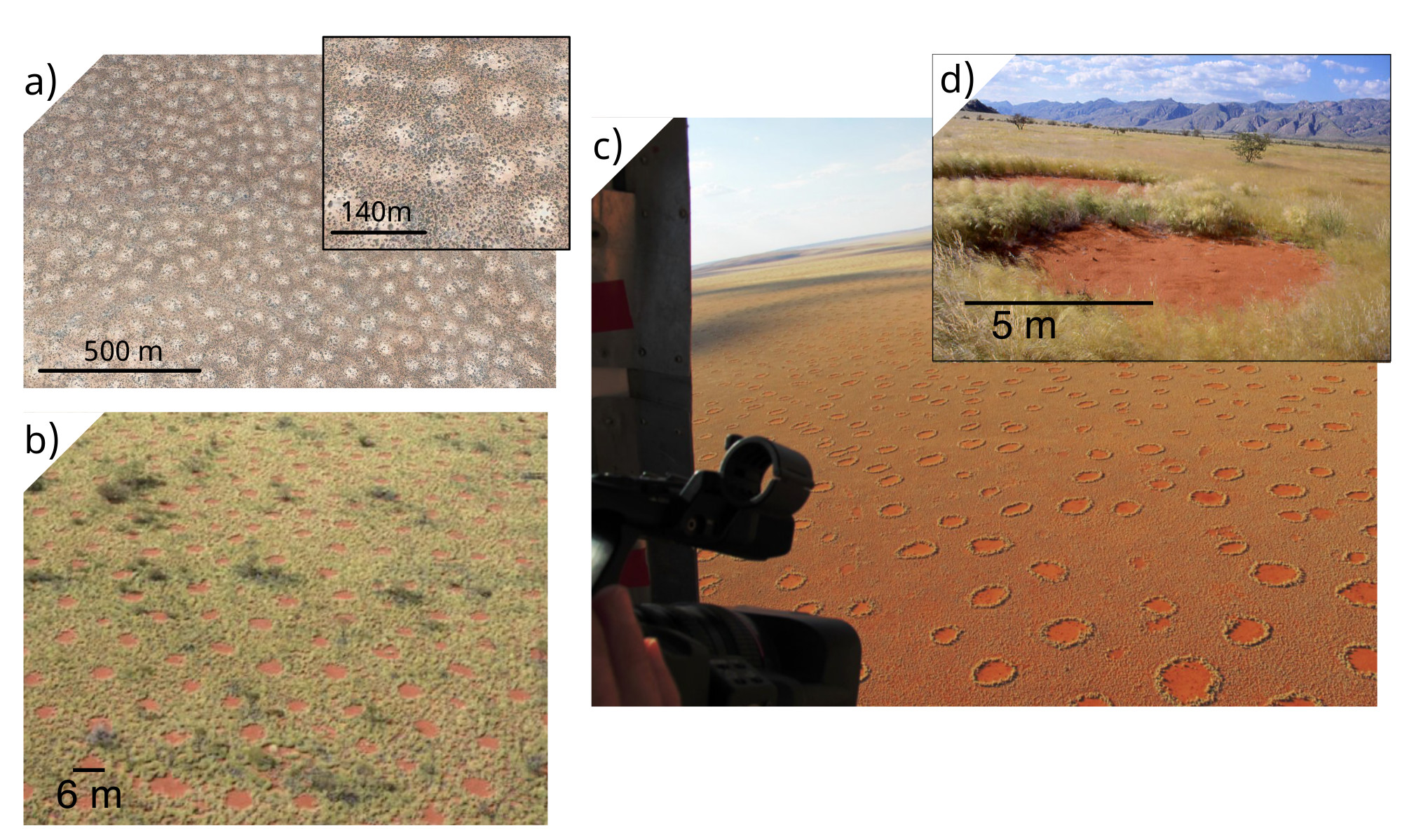
Figure 1: Field observations of gapped vegetation patterns. (a) North western Africa (Kenya, $0\textordmasculine 42^{\prime}16.61^{\prime\prime}$N, $40\textordmasculine 22^{\prime}19.06^{\prime\prime}$E ). (b) North west Australia (c,d) Pro-Namibia zone of the west coast of Southern Africa (c) Aerial photography: courtesy of Norbert Juergen. (d) Photography: courtesy of Johnny Vergeer .

Vegetation patterns are not necessarily periodic. They can be aperiodic and localized in space in the form of more or less circular patches surrounded by a bare soil [16, 17]. Localized vegetation structures is a patterning phenomenon that occurs under the same condition as symmetry-breaking instability. However, for a moderate level of aridity, they tend to spread and to invade the whole space available in a given landscape. This bifurcation is referred to as curvature instability that deforms the circular shape of localized patches and provokes a self-replication phenomenon that can take place even in strictly isotropic environmental conditions [18, 19, 20]. This curvature instability may lead to the formation of another type of morphologies, such as arcs and spiral like vegetation patterns [5].

We investigate the formation of gapped vegetation patterns under a strictly homogeneous environmental conditions. They consist either periodic or aperiodic distribution of spots of bare soil embedded in a uniform vegetation cover (see Fig. 1). By taking into account the effect of the crown/root allometry together with the facilitative and the competitive plant-to-plant interactions, we show that the homogeneous cover exhibits a symmetry-breaking instability leading the formation of spatially periodic distribution of gaps. We characterize first the formation of periodic gaps by drawing their bifurcation diagram. Then, we identify the range of the parameter where landscapes exhibit stable localized gaps. These structures are characterized by an exponentially decaying oscillatory tails, which stabilize a large number of gaps and clusters of them [21]. We establish a snaking bifurcation diagram associated with localized gaps. From the theory of dynamical systems point of view, the bifurcation diagram associated with gaps localized structure consists of two snaking curves: one describes gaps localized vegetation patterns within an odd number of gaps, the other corresponds to even a number of gaps. This type of gaps self-organization is often called homoclinic snaking bifurcation and have been intensively studied in the framework of the Swift-Hohenberg equation [22, 23, 24], see also a review paper [25] in the theme issue [26]. A paradigmatic Swift-Hohenberg equation has been derived in the context of plant ecology in vicinity of the critical point associated with bistability by Lefever and collaborators [3]. This model undergoes snaking bifurcations for both localized patches and gaps [27, 28].

The paper is organized as follows: In section 2, we present the model and analyze the uniformly covered states. In section 3, we analyzed and characterize the formation of gapped vegetation patterns in one and two-dimensions. In section 4 we study localized gaps, and analyze them in terms of the homoclinic snaking bifurcation in one dimension.

2 Interaction-redistribution model for the biomass evolution: nonlocal interactions and crown/roots allometry

During more than two decades, several models have been proposed to investigate the formation of vegetation patterns and the associated self-organization phenomenon. These approaches can be classified into three categories. The first is the generic interaction-redistribution model based on the relationship between the structure of individual plants and the facilitation-competition plant-to-plant interactions existing within plant communities. This modeling considers a single biomass variable [1]. The second is based on reaction-diffusion type of modeling. This approach focuses on the influence of water transport by below ground diffusion and/or above ground run-off [29, 30, 12, 13, 14]. The third modeling approach is based on the stochastic processes that take into account the role of environmental randomness as a mechanism of noise induced symmetry-breaking transitions [31, 32]. In what follows, let us consider the first modeling approach, the interaction-redistribution model [33],

$$\partial_{t}b=F_{f}\left(b+dF_{d}\right)\left(1-F_{c}\right)-\mu b,$$ (1)

where $b=b({\bf r},t)$ is the biomass density at the position ${\bf r}=(x,y)$ and the time $t$. The functions $F_{f}$, $F_{c}$, and $F_{d}$ account for facilitation, competition, and seed dispersion mechanisms of the plant-to-plant feedbacks, respectively. The parameter $\mu$ models the aridity, that is, the plant mortality, which is mostly attributed to adverse environmental conditions. The explicit forms of the nonlocal functions $F_{f,c,d}$, are

$$F_{f}=\exp{\left(\frac{1}{C_{1}}\int e^{-\frac{\left|{\bf r}^{\prime}\right|}{L_{1}}}b({\bf r}+{\bf r}^{\prime},t)\ d{\bf r}^{\prime}\right)}, F_{c}=\frac{\int e^{-\frac{|{\bf r}^{\prime}|}{L_{2}}}b({\bf r}+{\bf r}^{\prime},t)\ d{\bf r}^{\prime}}{\int e^{-\frac{|{\bf r}^{\prime}|}{L_{2}}}\ d{\bf r}^{\prime}},$$

$$\qquad F_{d} = \frac{1}{C_{d}}\int e^{-\frac{{\bf r}^{\prime 2}}{L_{d}^{2}}}b({\bf r}^{\prime}+{\bf r},t)\ d{\bf r}^{\prime}.$$

Normalization factors are $C_{1}=2L_{a}$, and $C_{d}=\sqrt{\pi}L_{d}$ for one-dimensional systems, and $C_{1}=2\pi L_{a}^{2},$ and $C_{d}=\pi L_{d}^{2}$ for two-dimensional systems. $L_{a}$ is the effective radius of the surface that occupies a mature plant. However, ecosystems not only comprise mature plants but also classes of different ages. Indeed, the age, the crown size, and root sphere are different from each plant. Mature and bigger plants require a higher amount of water and nutrients. Young and smaller plants explore through their roots smaller territories for the uptake of water and nutrients. In other words, the allometric factor plays an important role in phyto-societal behaviors that governs the range of facilitative and competitive interactions during development of plants. For a given spatial point, the effective ranges of the facilitative and the competitive interactions depend on the biomass density. The range of influence of young plants (associated with lower biomass) must be smaller than the influence range of the older ones (associated with higher biomass). The allometric factor is a statistical constant that has been established to be $p=1/3$ by measuring the relative size of the above-ground (crown) and below-ground (rhizosphere) structures for the plant C. micranthum in Neger [2, 3]. The effective ranges of interaction take the form [14, 34]

$$L_{1,2}=L_{1,2}^{0}b^{p}$$ (2)

where $p$ is the allometric factor and $L_{1,2}^{0}$ are constants. In the absence of the allometry, i.e., $p=0$ the effective ranges of both facilitative and competitive interactions are independent of the biomass density. However as we shall see, when $p\neq 0$, the allometry modifies the position of the critical point associated with bistability and induces a new branch of low biomass [3, 33].

The homogeneous steady states, $b({\bf r},t)=b_{0}$, corresponding to the homogenous covers are solution of Eq. (1). The trivial solution is the bare state $b_{0}=0$, represents a territory totally devoid of vegetation. The barren state obviously exists for all values of the parameters. Homogeneous covers satisfy the following equation

$$\mu=\exp\left(\Gamma^{n}b_{0}^{np+1}\right)\left(1+d\right)\left(1-b_{0}\right),$$ (3)

where $\Gamma\equiv L_{1}/L_{a}$ and $n$ is the dimension of the system ($n=1$ corresponds to 1D and $n=2$ corresponds to 2D). The dimension of the system and the allometric factor impact the homogeneous steady state curves. Depending on the parameter values, one can find monostable and bistable regimes, between these spatially homogeneous states. The coordinates of this second-order critical point marking the onset of a hysteresis loop is obtained by satisfying simultaneously the conditions

$$\frac{\partial\mu}{\partial b_{0}}=0~{}~{}~{}~{}\mbox{and}~{}~{}~{}~{}\frac{\partial^{2}\mu}{\partial b_{0}^{2}}=0,$$ (4)

with $\mu$ satisfies Eq. (3). The two conditions Eq. (4) allow to estimate the coordinate of the critical point associated with bistability $(\Gamma_{c},\mu_{c},b_{c})$.

In the absence of the allometry $p=0$, i.e., when all plants are mature, two regimes must be distinguished according to the value of the $\Gamma=L_{1}/L_{a}$ parameter. If $\Gamma<1$ (monostable regime), the uniformly vegetated cover exists only in the range $0<\mu<1$. In this parameter range, the biomass decreases monotonously with aridity and vanishes at $\mu=1+d$. For larger aridity levels, i.e., $\mu>1+d$ only the barren state exists as shown in Fig. 2(a). If $\Gamma>1$ (bistable regime), the state of the uniformly vegetated cover extends up to the tipping point (saddle-node bifurcation) as shown in Fig. 2(a,b). This means that when increasing the facilitative interaction range, vegetation community can survive while individual plants can not. This situation corresponds to the vegetation systems presented in Fig. 2(a) in a one-dimensional system and in Fig. 2(b) for two-dimensional settings. If $\Gamma=1$, the system reaches the second-order critical point marking the onset of a hysteresis loop. The coordinate of this critical point is $\mu_{c}=1+d$ and $b_{c}=0$. In this case, spatial oscillations around $b_{c}=0$ are physically excluded. When, however, we take into account the allometry, the coordinate of the critical point associated with the nascent bistability occurs with a finite biomass ($b_{c}\neq 0$), as shown in Figs. 2(c,d). Another important consequence of the allometry is that a new stable state with low biomass density is possible as shown in Fig. 2(d). Therefore, there is a parameter range where the system exhibits tristability. Besides the stable barren state, the high and low biomass covers can coexist for the same values of system parameters. From Figs. 2, we infer that all curves, in the $\left(\mu,b_{0}\right)$-plane, coincide at the same point $\left(\mu=1+d,b_{0}=0\right)$. The slope at this point is explicitly given by $\partial\mu/\partial b_{0}=-\left(1+d\right)$, which is independent of the other parameter values. Dashed curves correspond to unstable solutions, while continuous curves denote solutions that are stable with respect to spatially homogeneous perturbations. In the next section, we will perform the linear stability analysis of the homogeneous covers with respect to spatially inhomogeneous perturbations.

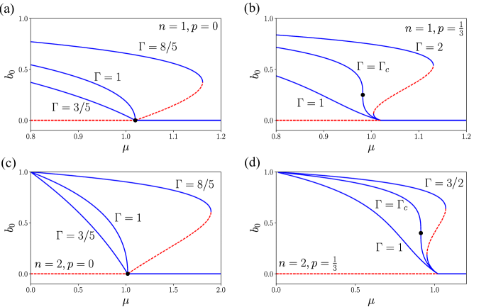
Figure 2: Homogeneous steady states solutions of Eq. (3), for $d=0.02$. The barren state $b_{0}=0$ is unstable for $\mu<1+d$; stable for $\mu>1+d$. Depending on the allometric exponent $p$, the spatial dimensions $n$, and the ratio $\Gamma$, the branch of vegetated solutions may or may not have an unstable part and a second section of stability. (left top panel) 1-d, no allometric effect $p=0$; (left bottom panel) 2-d, no allometric effect $p=0$; (right top panel) 1-d, allometric effect $p=1/3$; and (right bottom panel) 2-d, allometric effect $p=1/3$. Stability to sinusoidal perturbations is analyzed in another section.

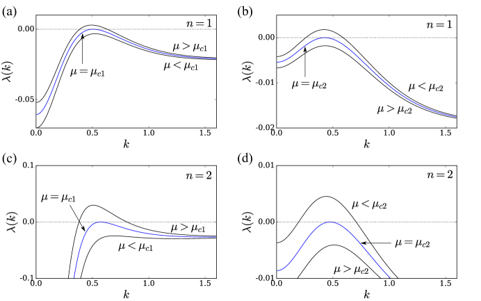
Figure 3: Stability of uniformly vegetated state to the introduction of small sinusoidal modulation, as parameter $\mu$ is varied, one ($n=1$) and two $(n=2)$ spatial dimensions. An allometric factor $p=1/3$ and a ratio $\Gamma=5/8$ were used in all the figures, so there is a range defined by two turning points where three vegetated homogeneous solutions exist. (left panels) Along the upper solution there is a bifurcation point $\mu_{c1}$ at which a critical mode $\exp(ikx)$ becomes unstable and its growth exponent $\lambda(k)$ becomes positive. (right panels) Along the lower solution there is also a bifurcation point $\mu_{c2}$ at which a mode becomes unstable. Other parameters are $L_{a}=5/4$, $L_{1}=2$, $L_{2}=2.8125$, $L_{d}=2.5$ and $d=0.02$.

3 Linear stability analysis and vegetation pattern formation

3.1 Linear stability analysis

We perform the linear stability analysis of the homogeneous steady state solutions of Eq. (3) with respect to small spatially inhomogeneous fluctuations around the homogeneous steady states; $b_{0}$; of the form

$$b({\bf r},t)=b_{0}+\delta b({\bf r},t),$$ (5)

with $\delta b({\bf r},t)\ll 1$. Replacing Eq. (5) into Eq. (1), and linearizing with respect to $\delta b({\bf r},t)$, one obtains a linear equation of the form $\partial_{t}\delta b({\bf r},t)=\mathcal{L}\delta b({\bf r},t)$. If all the eigenvalues of operator $\mathcal{L}$ have a negative real part, the homogeneous state $b_{0}$ is stable, otherwise, it is unstable. Since the system is invariant under spatial translations, the linear operator $\mathcal{L}$ is diagonal in the Fourier basis $\mathcal{L}\exp\left(i{\bf k}\cdot{\bf r}\right)=\lambda(k)\exp\left(i{\bf k}\cdot{\bf r}\right)$. The function $\lambda(k)$, often called the spectrum, is always real for the approach based on the interaction-redistribution model Eq. (1) and therefore time oscillations around the homogeneous covers are therefore excluded. The spectrum only depends on the modulus of the wavevector ${\bf k}$. This is because the system is isotropic in both $x$ and $y$ direction, and then there is no preferred direction in the plane $(x,y)$. This spectrum can be computed analytically but the obtained expressions for both the threshold as well for the most unstable wavelength at the symmetry breaking instability are cumbersome. The plot of the spectrum as a function of the wavenumber is shown in Fig. 3 for $p=1/3$.

It shows the spectrum for the upper branches (left panels), that is, the higher density state, and the lower branches (right panels), that is, the lower density state. These spectra have been computed in one (top panels) and two (bottom panels) dimensions and for $p=1/3$. As we see, from Fig. 3, there exist a range of aridity parameter, $\mu_{c1}<\mu<\mu_{c2}$, where the homogeneous cover is unstable and giving rise to the formation of a periodic vegetation pattern.

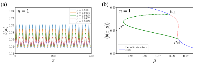
Figure 4: One dimensional periodic structure. (a) Representation of homogeneous solution and the spatially periodic solution that are born at the two bifurcation points, as computed with finite differences and pseudo-arclength continuation algorithm. (b) Heterogeneous solutions for different values of aridity $\mu$. As parameter $\mu$ decreases, the amplitude of the stable periodic profile grows. Other parameters are $L_{a}=5/4$, $L_{1}=2$, $L_{2}=2.8125$, $L_{d}=2.5$, and $d=0.02$.

3.2 Vegetation pattern formation

To analyze the formation of vegetation patterns that are spontaneously triggered by the symmetry-breaking instability, we first compute the spatially periodic structure in one spatial dimension $(n=1)$. For this purpose we use a continuation method. More precisely, we numerically determine the branches of nonlinear solutions of Eq. (1). The stability analysis of these solutions is performed with continuation software (AUTO), which is based on the pseudo-arclength method [35]. The results are summarized in Fig. 4, where the spatially periodic profiles of the biomass are plotted for different values of the level of aridity $\mu$. From this figure, we see that as parameter $\mu$ is decreases, the biomass grows. The bifurcation diagrams associated with these solutions are plotted as a function of the level of the aridity in Fig. 4b. When increasing the level of aridity the high biomass cover is stable in the range $0<\mu<\mu_{c1}$. At $\mu=\mu_{c1}$, the homogeneous high biomass cover becomes unstable with respect to spatially symmetry-breaking instability. From this bifurcation point $\mu=\mu_{c1}$, a periodic solution emerges spontaneously as shown in Fig. 4b. When increasing further the aridity, the homogeneous lower biomass state stabilizes due to the second spatial symmetry instability at $\mu=\mu_{c2}$ (see Fig. 4b). The periodic solutions in the vicinity of $\mu=\mu_{c2}$ appear supercritical with small amplitude. However, the bifurcation at $\mu=\mu_{c1}$ is subcritical. In this case, namely in the range $\mu^{*}<\mu<\mu_{c1}$, the system exhibits a coexistence between a periodic gapped patterns and the homogeneous high biomass cover. As we will see in the next section, the coexistence is prerequisite conditions for the formation of localized gaps. For $\mu>\mu_{c2}$, the low biomass cover is stable until the system reaches the barren state at $\mu=1+d$. For $\mu>1+d$, only the barren state is stable.

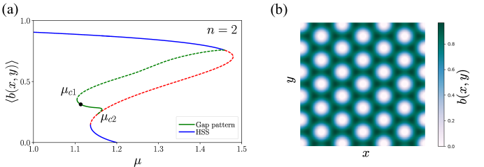
Figure 5: (left panel) Branches of solutions with hexagonal symmetry computed with a Fourier expansion and a pseudo-arclength continuation algorithm. Parameter values: $p=1/3,L_{a}=5/4$, $L_{1}=2$, $L_{2}=2.8125$, $L_{d}=2.5$ and $d=0.02$. (right panel) Stable hexagonal pattern of gaps for $\mu=1.11$ (indicated with black dot in left panel).

In the two-dimensional system ($n=2$), when increasing the aridity parameter, the first vegetation pattern that appears is the periodic distribution of gaps forming a hexagonal structure as shown in Fig. 5. The bifurcation diagram associated with these two-dimensional solutions is plotted in Fig. 5. The results are obtained by using the continuation method in [35] that consist of assuming that the biomass is distributed in a periodic manner and the wavevectors define a finite hexagonal lattice that is conjugated to the spatial lattice generated from the basic hexagon.

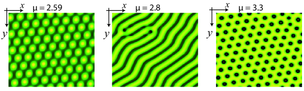
Figure 6: Generic sequence of vegetation patterns obtained from model Eq. (1). Aridity parameter is increases from left to right. other parameters are $d=0.5$, $p=0$, $L_{a}=5/4$, $L_{1}=2$, $L_{2}=2.8125$, and $L_{d}=2.5$.

After having fully characterized the formation of periodic distribution of gaps as a function of the aridity parameter, we recover the generic sequence gaps $\iff$ stripes $\iff$ spots as shown in Fig. 6. These ecological states in arid landscapes possess an overlap domain of stability as shown analytically in weak gradient approximation [11].

4 Localized gaps and snaking bifurcation

Localized structures and localized patterns are a well documented phenomenon, concerning almost all fields of natural science including chemistry, biology, ecology, physics, fluid mechanics, and optics [36, 37, 38, 39, 40, 41]. Localized vegetation patches and gaps belong to the class of stationary and spatially localized patterns. They consist either of localized vegetation patches distributed on bare soil [16, 42] or, on the contrary, of localized spots of bare soil embedded in an otherwise uniform vegetation cover [21]. Localized patches or localized bare soil spots (often called fairy circles) can be either spatially independent, self-organized, or randomly distributed.

It is worth mentioning that fairy circles are striking examples attributed to this category of localized vegetation patterns [43]. Although, the mechanisms leading to their formation are still subject of debate among the scientific community. They have been interpreted as the result of a pinning front between a uniform plant distribution and a periodic hexagonal vegetation pattern [21]. Recent investigations support this interpretation [44, 45, 46]. On the other hand, fairy circles formation may result from front dynamics connecting a bare state and uniform plant distributions [47, 48, 49]. In all these works, the origin of fairy circle formation is intrinsic to the dynamics of the system. This means that the diameter of the fairy circle is determined rather by the parameters of the system and not by external effects, such as the presence of social insects or anisotropy. However, another theory based on external effects, such as termites or ants has been suggested [50, 51, 52, 53]. More recently, Tarnita and collaborators have shown that a combination of intrinsic and extrinsic effects could explain the origin of fairy circles [54].

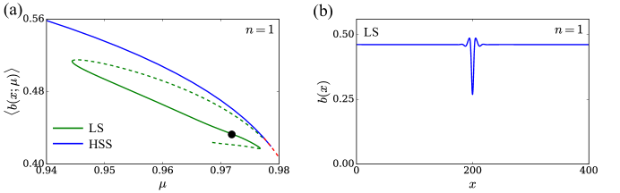
Figure 7: (left panel) Branch of localized solutions with odd number of gaps, born at the bifurcation point of the upper homogeneous branch. The vertical coordinate is the norm of the solution with respect to the homogeneous solution for that value of $\mu$. (right panel) Localized solution with a single gap. This solution is stable and corresponds to $\mu=0.972$ (black dot in left panel). Other parameters are $L_{a}=5/4$, $L_{1}=2$, $L_{2}=2.8125$, $L_{d}=2.5$, and $d=0.02$.

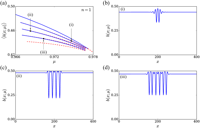
Figure 8: (left panel) Branch of localized solutions with even number of gaps, born at the bifurcation point of the upper homogeneous branch. The vertical coordinate is the norm of the solution with respect to the homogeneous solution for that value of $\mu$. (other three panels) Localized solutions with two, three and four gaps. These solutions are stable and correspond to $\mu=0.9754$, $\mu=0.9673$, and $\mu=0.9704$ (dots in left panel). Other parameters are $L_{a}=5/4$, $L_{1}=2$, $L_{2}=2.8125$, $L_{d}=2.5$, and $d=0.02$.

The bifurcation theory of localized structures developed for other extended models indicates that they are born at the same critical point as vegetation gapped periodic patterns, and they are unstable, gaining stability only after a fold. For instance a localized solution born at the bifurcation point of the upper branch will look like a small region of smaller density surrounded by a uniform region of density equal to the upper branch for that value of the aridity, essentially a gap. A localized gap pattern born at the lower branch will look like a bump surrounding by high biomass density (see Fig. 7).

Subsequent folds of the branch of localized solutions make them switch stability and add extra gaps or bumps. The complete bifurcation diagram, plotted using $\mu$ and the spatial average of $b(x)$, shows a complicated snaking diagram with an infinite number of folds as the patterns becomes more and more similar to the periodic solution. Note that there are two basic branches: one with an odd number of gaps, and other with an even number of gaps. We draw only the branch corresponding to odd number of gaps. We find numerically the first few folds of these two branches. These branches are displayed in Fig. 7 for single gap and Fig. 8 for clusters of odd number of gaps.

5 Conclusions

By using the generic interaction-redistribution model Eq.(1), we have analyzed ecological state transitions in stressed landscapes. We have shown that the allometry affects the homogeneous covers by : (i) shifting the critical point associated with bistability to a finite biomass density and (ii) by inducing a new branch of stable low biomass cover. We have shown that gaps are the first self-organized structure that appears when the level of the aridity is increased. We have attributed their formation to facilitative and competitive interactions between individual plants. We have recovered the generic sequence gaps $\iff$ bands or labyrinth $\iff$ spots. We have established the two-dimensional bifurcation diagram associated with periodic gapped vegetation patterns. To perform the analysis, we have used the continuation method based on the pseudo-arclength technique. Furthermore, we have fully analyzed the formation of localized gaps, and we have shown that they undergo a homoclinic snaking bifurcation.

Funding

This work was supported by a FONDECYT-Chile grant [1170669]. MT received support from the Fonds National de la Recherche Scientifique (Belgium).

References

References

- [1] R. Lefever, O. Lejeune, On the origin of tiger bush, Bull. Math. Biol. 59 (2) (1997) 263–294.
- [2] N. Barbier, P. Couteron, R. Lefever, V. Deblauwe, O. Lejeune, Spatial decoupling of facilitation and competition at the origin of gapped vegetation patterns, Ecology 89 (6) (2008) 1521–1531.
- [3] R. Lefever, N. Barbier, P. Couteron, O. Lejeune, Deeply gapped vegetation patterns: On crown/root allometry, criticality and desertification, J. Theor. Biol. 261 (2009) 194–209.
- [4] P. Couteron, F. Anthelme, M. Clerc, D. Escaff, C. Fernandez-Oto, M. Tlidi, Plant clonal morphologies and spatial patterns as self-organized responses to resource-limited environments, Philosophical Transactions of the Royal Society A: Mathematical, Physical and Engineering Sciences 372 (2027) (2014) 20140102.
- [5] M. Tlidi, M. Clerc, D. Escaff, P. Couteron, M. Messaoudi, M. Khaffou, A. Makhoute, Observation and modelling of vegetation spirals and arcs in isotropic environmental conditions: dissipative structures in arid landscapes, Philosophical Transactions of the Royal Society A: Mathematical, Physical and Engineering Sciences 376 (2135) (2018) 20180026.
- [6] R. M. Callaway, Positive interactions among plants, The Botanical Review 61 (4) (1995) 306–349.
- [7] R. M. Callaway, L. R. Walker, Competition and facilitation: a synthetic approach to interactions in plant communities, Ecology 78 (7) (1997) 1958–1965.
- [8] A. M. Turing, The chemical basis of morphogenesis, Philosophical Transactions of the Royal Society of London B: Biological Sciences 237 (641) (1952) 37–72.
- [9] I. Prigogine, R. Lefever, Symmetry breaking instabilities in dissipative systems. ii, Journal of Chemical Physics 48 (1968) 1695–1700.
- [10] O. Lejeune, M. Tlidi, A model for the explanation of vegetation stripes (tiger bush), J. Veg. Sci. 10 (1999) 201–208.
- [11] O. Lejeune, M. Tlidi, R. Lefever, Vegetation spots and stripes: dissipative structures in arid landscapes, International Journal of Quantum Chemistry 98 (2) (2004) 261–271.
- [12] J. von Hardenberg, E. Meron, M. Shachak, Y. Zarmi, Diversity of vegetation patterns and desertification, Physical Review Letters 87 (2001) 198101.
- [13] M. Rietkerk, J. van de Koppel, Regular pattern formation in real ecosystems, Trends in Ecology and Evolution 23 (3) (2008) 169.
- [14] E. Gilad, J. von Hardenberg, A. Provenzale, M. Shachak, E. Meron, Ecosystem engineers: From pattern formation to habitat creation, Phys. Rev. Lett. 93 (2004) 098105.
- [15] K. Gowda, H. Riecke, M. Silber, Transitions between patterned states in vegetation models for semiarid ecosystems, Phys. Rev. E 89 (2014) 022701.
- [16] O. Lejeune, M. Tlidi, P. Couteron, Localized vegetation patches: A self-organized response to resource scarcity, Phys. Rev. E 66 (2002) 010901.
- [17] M. Rietkerk, S.C. Dekker, P.C. De Ruiter, J van de Koppel, Self-organized patchiness and catastrophic shifts in ecosystems. Science, 305, (2004) 1926-1929.
- [18] I. Bordeu, M. G. Clerc, P. Couteron, R. Lefever, M. Tlidi, Self-replication of localized vegetation patches in scarce environments, Scientific reports 6 (2016) 33703.
- [19] I. Bordeu, M. Clerc, R. Lefever, M. Tlidi, From localized spots to the formation of invaginated labyrinthine structures in a swift–hohenberg model, Communications in Nonlinear Science and Numerical Simulation 29 (1-3) (2015) 482–487.
- [20] M. Tlidi, I. Bordeu, M. G. Clerc, D. Escaff, Extended patchy ecosystems may increase their total biomass through self-replication, Ecological indicators 94 (2018) 534–543.
- [21] M. Tlidi, R. Lefever, A. Vladimirov, On vegetation clustering, localized bare soil spots and fairy circles, Lecture Notes in Physics 751 (2008) 381–402.
- [22] P. Woods, A. Champneys, Heteroclinic tangles and homoclinic snaking in the unfolding of a degenerate reversible Hamiltonian–Hopf bifurcation, Physica D: Nonlinear Phenomena 129 (3-4) (1999) 147–170.
- [23] P. Coullet, C. Riera, C. Tresser, Stable static localized structures in one dimension, Physical review letters 84 (14) (2000) 3069.
- [24] M. G. Clerc, C. Falcon, Localized patterns and hole solutions in one-dimensional extended systems, Physica A: Statistical Mechanics and its Applications 356 (1) (2005) 48–53.
- [25] J. Burke, E. Knobloch, Homoclinic snaking: structure and stability, Chaos: An Interdisciplinary Journal of Nonlinear Science 17 (3) (2007) 037102.
- [26] M. Tlidi, M. Taki, T. Kolokolnikov, Introduction: dissipative localized structures in extended systems, 17, (2007) 037101.
- [27] A. Vladimirov, R. Lefever, M. Tlidi, Relative stability of multipeak localized patterns of cavity solitons, Physical Review A 84 (4) (2011) 043848.
- [28] G. Bel, A. Hagberg, E. Meron, Gradual regime shifts in spatially extended ecosystems, Theoretical Ecology 5 (4) (2012) 591–604.
- [29] C. A. Klausmeier, Regular and irregular patterns in semiarid vegetation, Science 284 (5421) (1999) 1826–1828.
- [30] R. HilleRisLambers, M. Rietkerk, F. van den Bosch, H. H. Prins, H. de Kroon, Vegetation pattern formation in semi-arid grazing systems, Ecology 82 (1) (2001) 50–61.
- [31] P. D’Odorico, F. Laio, L. Ridolfi, Patterns as indicators of productivity enhancement by facilitation and competition in dryland vegetation, Journal of Geophysical Research: Biogeosciences 111, no. G3 (2006).
- [32] L. Ridolfi, P. D’Odorico, F. Laio, Noise-induced phenomena in the environmental sciences, Cambridge University Press, 2011.
- [33] R. Lefever, J. Turner, A quantitative theory of vegetation patterns based on plant structure and the non-local F-KPP equation, Comptes Rendus Mecanique 340 (2012) 818–828.
- [34] E. Sheffer, H. Yizhaq, E. Gilad, M. Shachak, E. Meron, Why do plants in resource-deprived environments form rings?, Ecological complexity 4 (4) (2007) 192–200.
- [35] H. Li, Hexagonal Fourier-Galerkin methods for the two-dimensional homogeneous isotropic decaying turbulence, J. Math. Study 47 (1) (2014) 21–46.
- [36] F. T. Arecchi, S. Boccaletti, P. Ramazza, Pattern formation and competition in nonlinear optics, Physics Reports 318 (1-2) (1999) 1–83.
- [37] N. Akhmediev, A. Ankiewicz (Eds.), Dissipative solitons: from optics to biology and medicine, Springer Science & Business Media, 2008.
- [38] M. Tlidi, K. Staliunas, K. Panajotov, A. G. Vladimirov, M. G. Clerc, Localized structures in dissipative media: from optics to plant ecology, Philosophical Transactions of the Royal Society A: Mathematical, Physical and Engineering Sciences 372 (2014) 20140101.
- [39] M. Tlidi, M. G. Clerc, Nonlinear dynamics: Materials, theory and experiments, Springer Proceedings in Physics 173 (2016).
- [40] M. Tlidi, M. a. Clerc, K. Panajotov, Dissipative structures in matter out of equilibrium: from chemistry, photonics and biology, the legacy of Ilya Prigogine (part 1), 376 (2018) 20180114.
- [41] M. Tlidi, M. Clerc, K. Panajotov, Dissipative structures in matter out of equilibrium: from chemistry, photonics and biology, the legacy of Ilya Prigogine (part 2), 376 (2018) 20180276.
- [42] E. Meron, E. Gilad, J. von Hardenberg, M. Shachak, Y. Zarmi, Vegetation patterns along a rainfall gradient, Chaos, Solitons & Fractals 19 (2) (2004) 367–376.
- [43] M. Van Rooyen, G. Theron, N. Van Rooyen, W. Jankowitz, W. Matthews, Mysterious circles in the Namib desert: review of hypotheses on their origin, Journal of Arid Environments 57 (4) (2004) 467–485.
- [44] W. R. Tschinkel, The life cycle and life span of Namibian fairy circles, PloS one 7 (6) (2012) e38056.
- [45] M. D. Cramer, N. N. Barger, Are Namibian “fairy circles” the consequence of self-organizing spatial vegetation patterning?, PloS one 8 (8) (2013) e70876.
- [46] S. Getzin, K. Wiegand, T. Wiegand, H. Yizhaq, J. von Hardenberg, E. Meron, Adopting a spatially explicit perspective to study the mysterious fairy circles of Namibia, Ecography 38 (1) (2015) 1–11.
- [47] C. Fernandez-Oto, M. Tlidi, D. Escaff, M. Clerc, Strong interaction between plants induces circular barren patches: fairy circles, Philosophical Transactions of the Royal Society A: Mathematical, Physical and Engineering Sciences 372 (2014) 20140009.
- [48] C. Fernandez-Oto, M. Clerc, D. Escaff, M. Tlidi, Strong nonlocal coupling stabilizes localized structures: an analysis based on front dynamics, Physical Review Letters 110 (17) (2013) 174101.
- [49] D. Escaff, C. Fernandez-Oto, M. Clerc, M. Tlidi, Localized vegetation patterns, fairy circles, and localized patches in arid landscapes, Physical Review E 91 (2) (2015) 022924.
- [50] T. Becker, S. Getzin, The fairy circles of Kaokoland (north-west Namibia) origin, distribution, and characteristics, Basic and Applied Ecology 1 (2000) 149–159.
- [51] M. D. Picker, V. Ross-Gillespie, K. Vlieghe, E. Moll, Ants and the enigmatic Namibian fairy circles–cause and effect?, Ecological Entomology 37 (1) (2012) 33–42.
- [52] N. Juergens, The biological underpinnings of Namib desert fairy circles, Science 339 (6127) (2013) 1618–1621.
- [53] J. A. Bonachela, R. M. Pringle, E. Sheffer, T. C. Coverdale, J. A. Guyton, K. K. Caylor, S. A. Levin, C. E. Tarnita, Termite mounds can increase the robustness of dryland ecosystems to climatic change, Science 347 (6222) (2015) 651–655.
- [54] C. E. Tarnita, J. A. Bonachela, E. Sheffer, J. A. Guyton, T. C. Coverdale, R. A. Long, R. M. Pringle, A theoretical foundation for multi-scale regular vegetation patterns, Nature 541 (7637) (2017) 398.