Singular Value Decomposition in Sobolev Spaces: Part II

Abstract.

Under certain conditions, an element of a tensor product space can be identified with a compact operator and the singular value decomposition (SVD) applies to the latter. These conditions are not fulfilled in Sobolev spaces. In the previous part of this work (part I), we introduced some preliminary notions in the theory of tensor product spaces. We analyzed low-rank approximations in $H^{1}$ and the error of the SVD performed in the ambient $L^{2}$ space.

In this work (part II), we continue by considering variants of the SVD in norms stronger than the $L^{2}$-norm. Overall and, perhaps surprisingly, this leads to a more difficult control of the $H^{1}$-error. We briefly consider an isometric embedding of $H^{1}$ that allows direct application of the SVD to $H^{1}$-functions. Finally, we provide a few numerical examples that support our theoretical findings.

1. Introduction

A function $u$ in the tensor product $H=H_{1}\otimes H_{2}$ of two Hilbert spaces $H_{1}$ and $H_{2}$ may be identified with a compact operator $T_{u}:H_{2}\rightarrow H_{1}$. This identification is possible when the norm on $H$ is not weaker than the injective norm, i.e., in a certain sense the norm on $H$ is compatible with the norms on $H_{1}$ and $H_{2}$. In such a case we can decompose $u$ as

(1.1) $$u=\sum_{k=1}^{\infty}\sigma_{k}\psi_{k}\otimes\phi_{k},$$

for a non-negative non-increasing sequence $\{\sigma_{k}\}_{k\in\mathbb{N}}$ and orthonormal systems $\{\psi_{k}\}_{k\in\mathbb{N}}\subset H_{1}$ and $\{\phi_{k}\}_{k\in\mathbb{N}}\subset H_{2}$. This is the well known singular value decomposition (SVD) and it provides low-rank approximations via

$$\inf_{\operatorname{rank}\left(v_{r}\right)\leq r}\left\|u-u_{r}\right\|^{2}_{H}=\left\|u-\sum_{k=1}^{r}\sigma_{k}\psi_{k}\otimes\phi_{k}\right\|^{2}_{H}=\sum_{k=r+1}^{\infty}\sigma_{k}^{2},$$

if, e.g., $\|\cdot\|_{H}$ is the canonical norm on a Hilbert tensor space.

If $H$ is the Sobolev space of once weakly differentiable functions, the above assumption is not satisfied and there is no SVD for a function $u\in H^{1}$ in general. The focus of this work is to explore variants of the SVD in different ambient spaces in the $H^{1}$-norm. In part I, we showed that low-rank approximations in the Tucker format in $H^{1}$ exist. More precisely,

Theorem 1.1.

$\mathcal{T}_{\boldsymbol{r}}\left({}_{a}\bigotimes_{j=1}^{d}H^{1}(\Omega_{j})\right)$ is weakly closed and therefore proximinal in $H^{1}(\Omega)$.

We also showed under which conditions

$$u\in{}_{\|\cdot\|_{1}}\bigotimes_{j=1}^{d}U^{\min}_{j}(u),$$

i.e., $u$ belongs to the tensor product of its minimal subspaces. Finally, we analyzed the $H^{1}$-error of the $L^{2}$-SVD for a general order $d\geq 2$.

In this part, we consider the intersection space structure of $H^{1}$

$$H^{1}(\Omega_{1}\times\Omega_{2})=\bigg{(}H^{1}(\Omega_{1})\otimes L^{2}(\Omega_{2})\bigg{)}\cap\bigg{(}L^{2}(\Omega_{1})\otimes H^{1}(\Omega_{2})\bigg{)}=:H^{(1,0)}\cap H^{(0,1)}.$$

We analyze the $H^{1}$-error of the $H^{(1,0)}$- and $H^{(0,1)}$-SVDs. We also consider an isometric embedding of $H^{1}$ into a space which allows the direct application of the SVD.

The paper is organized as follows. In Section 2, we consider the $H^{(1,0)}$- and $H^{(0,1)}$-SVDs and generalizations to higher dimensions. In Section 3, we consider the SVD in higher-dimensional spaces of mixed smoothness, exponential sum approximations and an isometric embedding of $H^{1}$ that allows a direct application of the SVD. We conclude in Section 4 with some simple numerical experiments with different types of low-rank approximations. Section 5 summarizes the results of part I and part II.

2. SVD in $H^{(1,0)}$ and $H^{(0,1)}$

Before we proceed with analyzing SVDs in $H^{(1,0)}$ and $H^{(0,1)}$, we consider the corresponding singular values and compare them to $L^{2}$-singular values.

2.1. $H^{(1,0)}$ and $H^{(0,1)}$ Singular Values

We consider a function $u\in H^{1}(\Omega)$ as an element of the intersection space $u\in H^{(1,0)}\cap H^{(0,1)}.$ We first consider $u$ as a Hilbert Schmidt operator $u:L^{2}(\Omega_{2})\rightarrow H^{1}(\Omega_{1})$ defined by

$$u[w]=\int_{\Omega_{2}}u(\cdot,y)w(y)dy,\quad w\in L^{2}(\Omega_{2}).$$

The difference to simply viewing $u$ as an $L^{2}$ integral kernel arises when we consider the adjoint $u^{*}:H^{1}(\Omega_{1})\rightarrow L^{2}(\Omega_{2})$

$$u^{*}[v]=\int_{\Omega_{1}}u(x,\cdot)v(x)+\frac{\partial}{\partial x}u(x,\cdot)\frac{d}{dx}v(x)dx,\quad v\in H^{1}(\Omega_{1}).$$

The corresponding left and right singular functions $\psi_{k}^{1}\in H^{1}(\Omega_{1})$ and $\phi_{k}^{0}\in L^{2}(\Omega_{2})$ are respectively given by

$$uu^{*}[\psi_{k}^{1}]=\int_{\Omega_{2}}u(\cdot,y)\int_{\Omega_{1}}u(x,y)\psi_{k}^{1}(x)+\frac{\partial}{\partial x}u(x,y)\frac{d}{dx}\psi_{k}^{1}(x)dxdy=\lambda^{10}_{k}\psi_{k}^{1},$$

and

$$u^{*}u[\phi_{k}^{0}] =\int_{\Omega_{1}}u(x,\cdot)\int_{\Omega_{2}}u(x,y)\phi_{k}^{0}(y)dydx$$

(2.1) $$+\int_{\Omega_{1}}\frac{\partial}{\partial x}u(x,\cdot)\int_{\Omega_{2}}\frac{\partial}{\partial x}u(x,y)\phi_{k}^{0}(y)dydx=\lambda^{10}_{k}\phi_{k}^{0},$$

with the corresponding singular values $\sigma_{k}^{10}=\sqrt{\lambda_{k}^{10}}$ sorted in decreasing order. Note that, unlike in the previous subsection, in general $\phi_{k}^{0}\not\in H^{1}(\Omega_{2})$. To guarantee this we would have to require $u\in H^{1}_{\text{mix}}(\Omega)$. This means that the sum $u_{r}=\sum_{k=1}^{r}\sigma^{10}_{k}\psi_{k}^{1}\otimes\phi_{k}^{0}$ does not make sense in $H^{1}(\Omega)$ in general, only in $H^{(1,0)}$.

Similarly, we can interpret $u\in H^{1}(\Omega)$ as a Hilbert Schmidt operator
$u:H^{1}(\Omega_{2})\rightarrow L^{2}(\Omega_{1})$ defined by

$$u[w]=\int_{\Omega_{2}}u(\cdot,y)w(y)+\frac{\partial}{\partial y}u(\cdot,y)\frac{d}{dy}w(y)dy,\quad w\in H^{1}(\Omega_{2}),$$

with an adjoint $u^{*}:L^{2}(\Omega_{1})\rightarrow H^{1}(\Omega_{2})$ given by $u^{*}[v]=\int_{\Omega_{1}}u(x,\cdot)v(x)dx,\quad v\in L^{2}(\Omega_{1}).$ The corresponding singular functions $\psi_{k}^{0}\in L^{2}(\Omega_{1})$ and $\phi_{k}^{1}\in H^{1}(\Omega_{2})$ satisfy

$$uu^{*}[\psi_{k}^{0}] =\int_{\Omega_{2}}u(\cdot,y)\int_{\Omega_{1}}u(x,y)\psi_{k}^{0}(x)dxdy$$

$$+\frac{\partial}{\partial y}u(\cdot,y)\int_{\Omega_{1}}\frac{\partial}{\partial y}u(x,y)\psi_{k}^{0}(x)dxdy=\lambda^{01}_{k}\psi_{k}^{0},$$

and

(2.2) $$u^{*}u[\phi_{k}^{1}]=\int_{\Omega_{1}}u(x,\cdot)\int_{\Omega_{2}}u(x,y)\phi_{k}^{1}(y)+\frac{\partial}{\partial y}u(x,y)\frac{d}{dy}\phi_{k}^{1}(y)dydx=\lambda^{01}_{k}\phi_{k}^{1},$$

where $\sigma_{k}^{01}=\sqrt{\lambda_{k}^{01}}$ are the corresponding singular values, sorted in decreasing order. We make the following immediate observation.

Proposition 2.1.

Let $u\in H^{1}(\Omega)$ and let $\sum_{k=1}^{\infty}\sigma_{k}^{00}\psi_{k}\otimes\phi_{k}$, $\sum_{k=1}^{\infty}\sigma_{k}^{10}\psi^{1}_{k}\otimes\phi^{0}_{k}$ and $\sum_{k=1}^{\infty}\sigma_{k}^{01}\psi^{0}_{k}\otimes\phi^{1}_{k}$ be the SVD of $u$ interpreted as an element of $H^{(0,0)}$, $H^{(1,0)}$ and $H^{(0,1)}$ respectively. Then, we have for all $r\geq 0$

$$\sum_{k=r+1}^{\infty}(\sigma_{k}^{00})^{2} \leq\sum_{k=r+1}^{\infty}(\sigma_{k}^{10})^{2}\leq\sum_{k=r+1}^{\infty}(\sigma_{k}^{00})^{2}\|\psi_{k}\|_{1}^{2},$$

$$\sum_{k=r+1}^{\infty}(\sigma_{k}^{00})^{2} \leq\sum_{k=r+1}^{\infty}(\sigma_{k}^{01})^{2}\leq\sum_{k=r+1}^{\infty}(\sigma_{k}^{00})^{2}\|\phi_{k}\|_{1}^{2}.$$

Proof.

The first statement is given by

$$\sum_{k=r+1}^{\infty}(\sigma^{10}_{k})^{2} =\inf_{v\in\mathcal{R}_{r}(H^{1}(\Omega_{1}){}_{a}\otimes L^{2}(\Omega_{2}))}\|u-v\|_{(1,0)}^{2}$$

$$\geq\inf_{v\in\mathcal{R}_{r}(L^{2}(\Omega_{1}){}_{a}\otimes L^{2}(\Omega_{2}))}\|u-v\|_{(0,0)}^{2}=\sum_{k=r+1}^{\infty}(\sigma^{00}_{k})^{2},$$

and

$$\sum_{k=r+1}^{\infty}(\sigma^{10}_{k})^{2} =\inf_{v\in\mathcal{R}_{r}(H^{1}(\Omega_{1}){}_{a}\otimes L^{2}(\Omega_{2}))}\|u-v\|^{2}_{(1,0)}\leq\Big{\|}u-\sum_{k=1}^{r}\sigma_{k}^{00}\psi_{k}\otimes\phi_{k}\Big{\|}_{(1,0)}^{2}$$

$$=\sum_{k=r+1}^{\infty}(\sigma_{k}^{00})^{2}\|\psi_{k}\|_{1}^{2}.$$

Analogously for the second statement. ∎

Note that the upper bounds in Proposition 2.1 do not necessarily hold component-wise, i.e., the inequalities $\sigma_{k}^{10}\leq\sigma_{k}^{00}\|\psi_{k}\|_{1},$ do not hold in general. This is due to the fact that when estimating the injective norm

$$\left\|\sum_{k=r+1}^{\infty}\sigma_{k}^{00}\psi_{k}\otimes\phi_{k}\right\|_{\vee\left(H^{1}(\Omega_{1}),L^{2}(\Omega_{2})\right)},$$

the functions $\psi_{k}$ are not orthonormal in $H^{1}(\Omega_{1})$ and the sequence $\{\sigma_{k}^{00}\|\psi_{k}\|_{1}\}_{k\in\mathbb{N}}$ is not necessarily decreasing.

Naturally, we can ask whether we can derive a bound of the sort

$$\sum_{k=r+1}^{\infty}(\sigma_{k}^{00})^{2}\|\psi_{k}\|_{1}^{2}\lesssim\sum_{k=r+1}^{\infty}(\sigma_{k}^{10})^{2}\gamma(k),$$

for some sequence $\gamma(k)$. Though we do not believe this is possible without further assumptions, we can nonetheless improve the bounds. This indicates that indeed the quantities $\sigma_{k}^{10}$ and $\sigma_{k}^{00}\|\psi_{k}\|_{1}$ are closely related. This will later be confirmed by numerical observations.

Theorem 2.2.

Let $u\in H^{1}(\Omega)$ and assume the $L^{2}$-SVD $u=\sum_{k=1}^{\infty}\sigma_{k}^{00}\psi_{k}\otimes\phi_{k}$ converges in $H^{1}(\Omega)$. Then, we have

$$\sigma_{r}^{10} =\|\psi_{r}^{1}\|_{0}^{-1/2}\left(\sum_{k=1}^{\infty}(\sigma_{k}^{00})^{4}|\left\langle\psi_{r}^{1},\psi_{k}^{0}\right\rangle_{1}|^{2}\right)^{1/4}\geq\sigma_{r}^{00}\left(\frac{\left\langle\psi_{r}^{1},\psi_{r}\right\rangle_{1}}{\|\psi_{r}^{1}\|_{0}}\right)^{1/2},$$

$$\sigma_{r}^{01} =\|\phi_{r}^{1}\|_{0}^{-1/2}\left(\sum_{k=1}^{\infty}(\sigma_{k}^{00})^{4}|\left\langle\phi_{r}^{1},\phi_{k}^{0}\right\rangle_{1}|^{2}\right)^{1/4}\geq\sigma_{r}^{00}\left(\frac{\left\langle\phi_{r}^{1},\phi_{r}\right\rangle_{1}}{\|\phi_{r}^{1}\|_{0}}\right)^{1/2}.$$

Proof.

We consider the $L^{2}$-SVD $u=\sum_{k=1}^{\infty}\sigma_{k}^{00}\psi_{k}\otimes\phi_{k}$. $u$ is identified with an operator $u:L^{2}(\Omega_{2})\rightarrow H^{1}(\Omega_{1})$. For any $w\in L^{2}(\Omega_{2})$,
$u[w]=\sum_{k=1}^{\infty}\sigma_{k}^{00}\left\langle w,\phi_{k}\right\rangle_{0}\psi_{k},$ converges in $H^{1}(\Omega_{1})$ and for any $v\in H^{1}(\Omega_{1})$, $u^{*}[v]=\sum_{k=1}^{\infty}\sigma_{k}^{00}\left\langle v,\psi_{k}\right\rangle_{1}\phi_{k},$ convergences in $L^{2}(\Omega_{2})$. Thus,

$$uu^{*}[v] =\sum_{k=1}^{\infty}\sigma_{k}^{00}\left\langle\sum_{l=1}^{\infty}\sigma_{l}^{00}\left\langle v,\psi_{l}\right\rangle_{1}\phi_{l},\phi_{k}\right\rangle_{0}\psi_{k}$$

$$=\sum_{k=1}^{\infty}\sum_{l=1}^{\infty}\sigma_{k}^{00}\sigma_{l}^{00}\left\langle v,\psi_{l}\right\rangle_{1}\left\langle\phi_{l},\phi_{k}\right\rangle_{0}\psi_{k}$$

$$=\sum_{k=1}^{\infty}(\sigma_{k}^{00})^{2}\left\langle v,\psi_{k}\right\rangle_{1}\psi_{k}.$$

On the other hand, utilizing the $H^{(1,0)}$-SVD of $u$, we have
$uu^{*}[v]=\sum_{k=1}^{\infty}(\sigma_{k}^{10})^{2}\left\langle v,\psi_{k}^{1}\right\rangle\psi_{k}^{1},$ and thus

$$uu^{*}[v]=\sum_{k=1}^{\infty}(\sigma_{k}^{00})^{2}\left\langle v,\psi_{k}\right\rangle_{1}\psi_{k}=\sum_{k=1}^{\infty}(\sigma_{k}^{10})^{2}\left\langle v,\psi_{k}^{1}\right\rangle\psi_{k}^{1}.$$

Substituting $v=\psi_{r}^{1}$, we obtain $\sum_{k=1}^{\infty}(\sigma_{k}^{00})^{2}\left\langle\psi_{r}^{1},\psi_{k}\right\rangle_{1}\psi_{k}^{0}=(\sigma_{r}^{10})^{2}\psi_{r}^{1},$ since $\{\psi_{k}^{1}\}_{k\in\mathbb{N}}$ are $H^{1}(\Omega_{1})$-orthonormal. Finally, taking the $L^{2}(\Omega_{1})$-norm of both sides and since $\{\psi_{k}\}_{k\in\mathbb{N}}$ are $L^{2}(\Omega_{1})$-orthonormal, we obtain
$\sum_{k=1}^{\infty}(\sigma_{k}^{00})^{4}|\left\langle\psi_{r}^{1},\psi_{k}\right\rangle|^{2}=(\sigma_{r}^{10})^{4}\|\psi_{r}^{1}\|_{0}^{2}.$ The statement for $\sigma_{r}^{01}$ follows analogously by identifying $u$ with an operator from $H^{1}(\Omega_{2})$ to $L^{2}(\Omega_{1})$. This completes the proof. ∎

The factors in the bounds in Theorem 2.2 reflect how $\psi_{r}^{1}$, normalized in $H^{1}(\Omega_{1})$, scales w.r.t. $\psi_{r}$, normalized in $L^{2}(\Omega_{1})$. For instance, if $\{\psi_{r}\}_{r\in\mathbb{N}}$ behaves like Fourier or wavelet basis, then $\psi^{1}_{r}\sim\|\psi_{r}\|^{-1}_{1}\psi_{r}$. In this case, the right hand side in Theorem 2.2 evaluates to $\sigma_{r}^{00}\left(\frac{\left\langle\psi_{r}^{1},\psi_{r}\right\rangle_{1}}{\|\psi_{r}^{1}\|_{0}}\right)^{1/2}\sim\sigma_{r}^{00}\|\psi_{r}\|_{1}.$ This leads precisely to the upper bound of Proposition 2.1. Analogous conclusions hold when considering $\sigma_{r}^{00}$, $\phi_{r}^{1}$ and $\phi_{r}$.

Extending the results of this subsection to $d>2$ using HOSVD singular values and, e.g., the Tucker format is straightforward. Since we can consider matricizations w.r.t. to each $1\leq j\leq d$ separately, the analysis effectively reduces to the case $d=2$. Difficulties arise only when considering simultaneous projections in different components of the tensor product space. There we have to assume the rescaled singular values converge, as was done in part I of this work.

2.2. $H^{(1,0)}$ and $H^{(0,1)}$ projections

Given the singular functions
$\{\psi_{k}^{1}\}_{k\in\mathbb{N}}$ and $\{\phi^{1}_{k}\}_{k\in\mathbb{N}}$ associated with $H^{(1,0)}$ and $H^{(0,1)}$ SVDs of $u$ respectively, we consider the finite dimensional subspaces

(2.3) $$B^{1}_{r} :=\operatorname{span}\left\{\psi_{k}^{1}:1\leq k\leq r\right\}\subset U^{\min}_{1}(u),$$

$$B^{2}_{r} :=\operatorname{span}\left\{\phi_{k}^{1}:1\leq k\leq r\right\}\subset U^{\min}_{2}(u),$$

and the corresponding $H^{1}$-orthogonal projections

(2.4) $$P_{r}:H^{1}(\Omega_{1})\rightarrow B^{1}_{r},\quad Q_{r}:H^{1}(\Omega_{2})\rightarrow B^{2}_{r}.$$

The tensor product $P_{r}\otimes Q_{r}$ is well defined on $H^{1}(\Omega_{1})\otimes_{a}H^{1}(\Omega_{2})$, and on this space it holds

(2.5) $$P_{r}\otimes Q_{r}=(P_{r}\otimes\operatorname{id}_{2})(\operatorname{id}_{1}\otimes Q_{r})=(\operatorname{id}_{1}\otimes Q_{r})(P_{r}\otimes\operatorname{id}_{2}).$$

However, the interpretation is problematic when considering $P_{r}\otimes Q_{r}$ on the closure of $H^{1}(\Omega_{1})\otimes_{a}H^{1}(\Omega_{2})$ . Take, e.g., the projection $P_{r}\otimes\operatorname{id}_{2}$. This is an orthogonal projection on $H^{(1,0)}$ and we have $(P_{r}\otimes\operatorname{id}_{2})u=\sum_{k=1}^{r}\sigma_{k}^{10}\psi_{k}^{1}\otimes\phi_{k}^{0}.$ But in general $(P_{r}\otimes\operatorname{id}_{2})u\not\in H^{(0,1)},$ unless $u\in H^{1}(\Omega_{1})\otimes_{a}H^{1}(\Omega_{2})$. Thus, the subsequent application $\operatorname{id}_{1}\otimes Q_{r}$ does not necessarily make sense and is not continuous.

Notice the difference with the projections $P_{r}^{1}$ and $P_{r}^{2}$ for $L^{2}$-SVD from part I (for $d=2$ and $r_{1}=r_{2}=r$). First, we had $P_{r}^{1}\otimes\operatorname{id}_{2}u=\operatorname{id}_{1}\otimes P_{r}^{2}u=P^{1}_{r}\otimes P^{2}_{r}u,$ since both the left and right projections already give the best rank $r$ approximation in $L^{2}$. Second, we required only $L^{2}$-orthogonality, thus preserving $H^{1}$-regularity in the image. Thus, $P^{1}_{r}\otimes P^{2}_{r}$ made sense on $H^{1}(\Omega)$, although the sequence of projections does not necessarily converge in $H^{1}(\Omega)$. To that end, we had to additionally assume in part I the convergence of the rank-$r$ approximations $u_{r}$, or convergence of the rescaled $L^{2}$-singular values.

In the present case, although we obtain optimality in the stronger $\|\cdot\|_{(1,0)}$-norm, we lose convergence or possibly even boundedness in the $\|\cdot\|_{(0,1)}$-norm. Thus, we can ask ourselves if $P_{r}$ is bounded from $L^{2}(\Omega_{1})$ to $L^{2}(\Omega_{1})$, i.e., if $P_{r}\in\mathcal{L}\left(L^{2}(\Omega_{1}),L^{2}(\Omega_{1})\right)$?

Specifically, what are the minimal assumptions - if any - that we require in order to achieve this? The next example shows that indeed even for simple projections this property is not guaranteed.

Example 2.3.

Let $\Omega_{1}=(0,1)$ and consider the space $H_{0}^{1}(0,1)$. We know $H_{0}^{1}(0,1)\hookrightarrow C(0,1)$. Consider $g\in H_{0}^{1}(0,1)\rightarrow\mathbb{R}$ defined by $g[f]:=f(0.5),$ $\forall f\in H_{0}^{1}(0,1).$ Clearly, $g$ is a linear functional. Moreover, since any such $f$ is absolutely continuous, $g$ is bounded in the $\|\cdot\|_{1}$-norm. Thus, $g\in(H_{0}^{1}(0,1))^{*}$. By the Riesz representation theorem, there exists a unique $\tilde{g}\in H_{0}^{1}(0,1)$, such that $g[f]=\left\langle f,\tilde{g}\right\rangle_{1}$, for all $f\in H_{0}^{1}(0,1)$.

Define the one dimensional subspace $U=\operatorname{span}\left\{\tilde{g}\right\}$. The corresponding $H^{1}$-orthogonal projection $P$ is given by $Pv=\|\tilde{g}\|_{1}^{-2}\left\langle v,\tilde{g}\right\rangle_{1}\tilde{g}=\|\tilde{g}\|_{1}^{-2}v(0.5)\tilde{g}.$ Consider the sequence

$$v_{n}(x):=\begin{cases}1+(n+1)(x-0.5),&\;\text{if}\quad 0.5-\frac{1}{n+1}\leq x<0.5,\\ 1+(n+1)(0.5-x),&\;\text{if}\quad 0.5\leq x\leq 0.5+\frac{1}{n+1},\\ 0,&\;\text{otherwise},\end{cases}$$

$n\in\mathbb{N}$. Clearly, $v_{n}\in H_{0}^{1}(0,1)$ for any $n\in\mathbb{N}$, $\|v_{n}\|_{0}\leq\sqrt{\frac{2}{n+1}}\longrightarrow 0$, and $Pv_{n}=\|\tilde{g}\|_{1}^{-2}\tilde{g}\neq 0$, for all $n\in\mathbb{N}$. Thus, $P$ can not be continuous in $L^{2}$.

A closer look at the preceding example shows that such a function $\tilde{g}\in H_{0}^{1}(0,1)$ differentiated twice yields the delta distribution. Therefore, it can not be in $H^{2}(\Omega_{1})$. On the other hand, if the function has $H^{2}$-regularity, as the next statement shows, we can indeed obtain boundedness in $L^{2}$.

Lemma 2.4.

Let $u\in H^{1}(\Omega)$. In addition, assume the second unidirectional derivatives of $u$ exist in the distributional sense and are bounded, i.e., $\left\|\frac{\partial^{2}}{\partial x^{2}}u\right\|_{0}<\infty,$ $\left\|\frac{\partial^{2}}{\partial y^{2}}u\right\|_{0}<\infty.$ Finally, assume $u$ satisfies either zero Dirichlet or zero Neumann boundary conditions. Then, the projections defined in (2.4) can be bounded as

$$\|P_{r}v\|_{1} \leq\sqrt{2}\|v\|_{0}\left(\sum_{k=1}^{r}\|\psi_{k}^{1}\|_{0}^{2}+\left\|\frac{d^{2}}{dx^{2}}\psi_{k}^{1}\right\|_{0}^{2}\right)^{1/2},$$

$$\|Q_{r}w\|_{1} \leq\sqrt{2}\|w\|_{0}\left(\sum_{k=1}^{r}\|\phi_{k}^{1}\|_{0}^{2}+\left\|\frac{d^{2}}{dy^{2}}\phi_{k}^{1}\right\|_{0}^{2}\right)^{1/2}.$$

Proof.

One can easily verify that $\psi_{k}^{1}$ and $\phi_{k}^{1}$ are twice weakly differentiable for any $k\in\mathbb{N}$. For any $v\in H^{1}(\Omega_{1})$, we can write $P_{r}v=\sum_{k=1}^{r}\left\langle v,\psi_{k}^{1}\right\rangle_{1}\psi_{k}^{1}.$ The coefficients can be written as

$$\left\langle v,\psi_{k}^{1}\right\rangle_{1} =\int_{\Omega_{1}}v(x)\psi_{k}^{1}(x)dx+\int_{\Omega_{1}}\frac{d}{dx}v(x)\frac{d}{dx}\psi_{k}^{1}(x)dx$$

$$=\int_{\Omega_{1}}v(x)\psi_{k}^{1}(x)dx-\int_{\Omega_{1}}v(x)\frac{d^{2}}{dx^{2}}\psi_{k}^{1}(x)dx,$$

where the boundary term vanishes due to the boundary conditions. Thus, we get

$$\|P_{r}v\|_{1}^{2} =\sum_{k=1}^{r}|\left\langle v,\psi_{k}^{1}\right\rangle_{1}|^{2}\leq\sum_{k=1}^{r}\left(\|v\|_{0}\|\psi_{k}^{1}\|_{0}+\|v\|_{0}\left\|\frac{d^{2}}{dx^{2}}\psi_{k}^{1}\right\|_{0}\right)^{2}$$

$$\leq 2\|v\|_{0}^{2}\sum_{k=1}^{r}\left(\|\psi_{k}^{1}\|^{2}_{0}+\left\|\frac{d^{2}}{dx^{2}}\psi_{k}^{1}\right\|^{2}_{0}\right).$$

Analogously for $Q_{r}$. This completes the proof. ∎

Note that in principle the assumption on the boundary conditions can be replaced or avoided, as long as we can estimate the appearing boundary term. The assumption can be avoided entirely by using an estimate for the $L^{\infty}$-norm via the Gagliardo-Nirenberg inequality, although this would yield a crude estimate and dimension dependent regularity requirements.

Under the conditions of Lemma 2.4, we can assert that $P_{r}\otimes Q_{r}$ is indeed continuous. Since $\|\cdot\|_{(0,1)}$ is a uniform crossnorm

$$\|P_{r}\otimes Q_{r}\|_{(0,1)}=\|P_{r}\|_{0}\|Q_{r}\|_{1}\leq\sqrt{2}\left(\sum_{k=1}^{r}\|\psi_{k}^{1}\|_{0}^{2}+\left\|\frac{d^{2}}{dx^{2}}\psi_{k}^{1}\right\|_{0}^{2}\right)^{1/2},$$

and similarly for $\|\cdot\|_{(1,0)}$. Thus, $P_{r}\otimes Q_{r}\in\mathcal{L}\left(H^{1}(\Omega),H^{1}(\Omega)\right).$ By density, we can uniquely extend $P_{r}\otimes Q_{r}$ onto $H^{1}(\Omega)$ and the identity (2.5) holds.

One might argue that requiring $P_{r}$ and $Q_{r}$ to be continuous in $L^{2}$ is unnecessary, since we only need that the mappings $P_{r}\otimes\operatorname{id}_{2}:H^{1}(\Omega)\rightarrow H^{(0,1)},$ and $\operatorname{id}_{1}\otimes Q_{r}$ are continuous. The following example shows that indeed $P_{r}\otimes\operatorname{id}_{2}$ need not be continuous even on elementary tensor products, if $P_{r}$ is not $L^{2}$ continuous.

Example 2.5.

Take $P$ to be the projection from Example 2.3. Consider the same sequence $\{v_{n}\}_{n\in\mathbb{N}}\subset H_{0}^{1}(0,1)$ as in Example 2.3. Take another sequence $w_{n}\in H^{1}_{0}(0,1)$ as

$$w_{n}(y):=\begin{cases}(n+1)^{-1/2}+(n+1)^{1/2}(y-0.5),&\;\text{if}\quad 0.5-n^{-1}\leq y<0.5,\\ (n+1)^{-1/2}+(n+1)^{1/2}(0.5-y),&\;\text{if}\quad 0.5\leq y<0.5+n^{-1},\\ 0,&\;\text{otherwise}.\end{cases}$$

Then,

$$\|w_{n}\|_{0}^{2} \leq 2(n+1)^{-2},$$

$$\|w_{n}\|_{1}^{2} \leq 2(n+1)^{-2}+2(n+1)(n+1)^{-1}=2(n+1)^{-2}+2,$$

$$\|w_{n}\|_{1}^{2} \geq 2.$$

Thus, since $\|\cdot\|_{(0,1)}$ is a crossnorm

$$\|(P\otimes\operatorname{id}_{2})(v_{n}\otimes w_{n})\|_{(0,1)}=\|Pv_{n}\|_{0}\|w_{n}\|_{1}\geq 2\|Pv_{1}\|_{0}>0,\quad\forall n\in\mathbb{N}.$$

On the other hand

$$\|v_{n}\otimes w_{n}\|_{1}^{2}\leq\|v_{n}\otimes w_{n}\|_{(10)}^{2}+\|v_{n}\otimes w_{n}\|_{(01)}^{2}=\|v_{n}\|^{2}_{1}\|w_{n}\|^{2}_{0}+\|v_{n}\|^{2}_{0}\|w_{n}\|^{2}_{1}$$

$$\leq[2(n+1)^{-1}+2(n+1)][2(n+1)^{-2}]+[2(n+1)^{-1}][2(n+1)^{-2}+2]$$

$$=[4(n+1)^{-3}+4(n+1)^{-1}]+[4(n+1)^{-3}+4(n+1)^{-1}]\longrightarrow 0.$$

Hence, $P\otimes\operatorname{id}_{2}$ is not continuous on $H^{1}(\Omega)$ even on $H^{1}(\Omega_{1})\otimes_{a}H^{1}(\Omega_{2})$.

To summarize our findings, let us define the finite dimensional subspaces $W^{1}_{r}:=\operatorname{span}\left\{\psi_{k}^{0}:1\leq k\leq r\right\},$ $W^{2}_{r}:=\operatorname{span}\left\{\phi_{k}^{0}:1\leq k\leq r\right\},$ Under the assumptions of Lemma 2.4, $W_{r}^{1}\subset H^{1}(\Omega_{1})$ and $W_{r}^{2}\subset H^{1}(\Omega_{2})$. This can also be observed by, e.g., considering (2.1) and integrating the second term by parts. We can estimate the $H^{1}$ error as follows.

Theorem 2.6.

Let the assumptions of Lemma 2.4 be satisfied. Moreover, define the constants

$$L(r):=\sup_{v\in B^{1}_{r}}\frac{\|v\|_{1}}{\|v\|_{0}}\sup_{v\in B^{1}_{r}}\frac{\|v\|_{2}}{\|v\|_{1}},\quad R(r):=\sup_{w\in B^{2}_{r}}\frac{\|w\|_{1}}{\|w\|_{0}}\sup_{w\in B^{2}_{r}}\frac{\|w\|_{2}}{\|w\|_{1}}.$$

Then, the projection error is bounded as

$$\frac{1}{\sqrt{2}}\left(\sum_{k=r+1}^{\infty}(\sigma_{k}^{10})^{2}+(\sigma_{k}^{01})^{2}\right)^{1/2}\leq\left\|u-(P_{r}\otimes Q_{r})u\right\|_{1}$$

$$\leq\left(\sum_{k=r+1}^{\infty}(1+2r^{2}R(r)^{2})(\sigma_{k}^{10})^{2}+(1+2r^{2}L(r)^{2})(\sigma_{k}^{01})^{2}\right)^{1/2}.$$

Proof.

For the lower bound observe first that

$$\|u-(P_{r}\otimes Q_{r})u\|^{2}_{1}\geq\frac{1}{2}\left(\|u-(P_{r}\otimes Q_{r})u\|^{2}_{(1,0)}+\|u-(P_{r}\otimes Q_{r})u\|^{2}_{(0,1)}\right).$$

Since $P_{r}\otimes\operatorname{id}_{2}u$ is the optimal rank $r$ approximation in the $\|\cdot\|_{(1,0)}$-norm, we can further estimate

$$\|u-(P_{r}\otimes Q_{r})u\|^{2}_{(1,0)}\geq\|u-(P_{r}\otimes\operatorname{id}_{2})u\|^{2}_{(1,0)}=\sum_{k=r+1}^{\infty}(\sigma_{k}^{10})^{2},$$

and similarly for $\operatorname{id}_{1}\otimes Q_{r}$. This gives the lower bound.

For the upper bound, since $P_{r}\otimes\operatorname{id}_{2}$ is orthogonal in the $\|\cdot\|_{(1,0)}$-norm, we get

$$\|u-(P_{r}\otimes Q_{r})u\|^{2}_{(1,0)}$$

$$=\|u-(P_{r}\otimes\operatorname{id}_{2})u\|^{2}_{(1,0)}+\|P_{r}\otimes\operatorname{id}_{2}[u-(\operatorname{id}_{1}\otimes Q_{r})u]\|^{2}_{(1,0)}.$$

To estimate the latter term, recall that $(P_{r}\otimes\operatorname{id}_{2})u\in B_{r}^{1}\otimes_{a}W^{2}_{r}$. Thus, we can find some $\{v_{i}\}_{i=1}^{r}$ in $B^{1}_{r}$ and $\{w_{i}\}_{i=1}^{r}$ in $W^{2}_{r}$ such that

(2.6) $$e_{r}:=P_{r}\otimes\operatorname{id}_{2}[u-(\operatorname{id}_{1}\otimes Q_{r})u]=\sum_{k=1}^{r}v_{i}\otimes w_{i}.$$

Thus, we estimate further

$$\|e_{r}\|_{(1,0)}^{2} \leq\left(\sum_{k=1}^{r}\|v_{i}\|_{1}\|w_{i}\|_{0}\right)^{2}\leq\left(\sum_{k=1}^{r}L_{1}(r)\|v_{i}\|_{0}\|w_{i}\|_{1}\right)^{2},$$

where $L_{1}(r):=\sup_{v\in B^{1}_{r}}\frac{\|v\|_{1}}{\|v\|_{0}}.$ Taking the infimum over all representations (2.6) of $e_{r}$, we obtain $\|e_{r}\|_{(1,0)}^{2}\leq L_{1}(r)^{2}\|e_{r}\|^{2}_{\wedge(0,1)},$ where $\|\cdot\|_{\wedge(0,1)}$ is the projective norm on $L^{2}(\Omega_{1})\otimes_{a}H^{1}(\Omega_{2})$. Let $\{\sigma^{e}_{k}\}_{k=1}^{r}$ denote the singular values of $e_{r}:H^{1}(\Omega_{2})\rightarrow L^{2}(\Omega_{1})$. Then, since the projective norm corresponds to the nuclear norm of the operator $e_{r}$ (see also [5, Remark 4.116])

$$\|e_{r}\|^{2}_{\wedge(0,1)}\leq\left(\sum_{k=1}^{r}\sigma_{k}^{e}\right)^{2}\leq r\sum_{k=1}^{r}(\sigma_{k}^{e})^{2}=r\|e_{r}\|^{2}_{(0,1)}.$$

In summary, $\|e_{r}\|_{(1,0)}^{2}\leq L_{1}(r)^{2}r\|e_{r}\|_{(0,1)}^{2}.$ Finally, to bound $P_{r}\otimes\operatorname{id}_{2}$, we apply Lemma 2.4

$$\|P_{r}\otimes\operatorname{id}_{2}\|_{(0,1)} \leq\sqrt{2}\left(\sum_{k=1}^{r}\|\psi_{k}^{1}\|_{0}^{2}+\left\|\frac{d^{2}}{dx^{2}}\psi_{k}^{1}\right\|_{0}^{2}\right)^{1/2}$$

$$\leq\sqrt{2}\left(\sum_{k=1}^{r}\|\psi_{k}^{1}\|_{0}^{2}+\left\|\frac{d}{dx}\psi_{k}^{1}\right\|_{0}^{2}+\left\|\frac{d^{2}}{dx^{2}}\psi_{k}^{1}\right\|_{0}^{2}\right)^{1/2}$$

$$=\sqrt{2}\left(\sum_{k=1}^{r}\frac{\|\psi_{k}^{1}\|^{2}_{2}}{\|\psi_{k}^{1}\|^{2}_{1}}\right)^{1/2}\leq\sqrt{2}\sqrt{r}L_{2}(r),$$

since $\psi_{k}^{1}$ are $H^{1}$ normalized and $L_{2}(r):=\sup_{v\in B^{1}_{r}}\frac{\|v\|_{2}}{\|v\|_{1}}$. Thus,

$$\|u-(P_{r}\otimes Q_{r})u\|_{(1,0)}^{2} \leq\sum_{k=r+1}^{\infty}(\sigma_{k}^{10})^{2}+2L_{1}(r)^{2}L_{2}(r)^{2}r^{2}\|u-\operatorname{id}_{1}\otimes Q_{r}\|_{(0,1)}^{2}$$

$$=\sum_{k=r+1}^{\infty}(\sigma_{k}^{10})^{2}+2L(r)^{2}r^{2}\sum_{k=r+1}^{\infty}(\sigma_{k}^{01})^{2}.$$

Analogously we can estimate the $\|\cdot\|_{(0,1)}$ error. This completes the proof. ∎

To conclude this section, we extend the preceding result to $d>2$. Unfortunately, unlike in the case for higher-order $L^{2}$-SVD in part I, the upper bound will depend exponentially on $d$. When performing an $L^{2}$-SVD in $d$ dimensions, the corresponding one dimensional projectors are $L_{2}$-optimal. Thus, when considering the tensor product $\mathcal{P}_{\boldsymbol{r}}$ of the projectors w.r.t. the $\|\cdot\|_{e_{j}}$-norm for any $1\leq j\leq d$, only one factor in $\mathcal{P}_{\boldsymbol{r}}$ is sub-optimal.

On the other hand, when the corresponding projectors are $H^{1}$-optimal and we consider the tensor product $\mathcal{P}_{\boldsymbol{r}}$ of the projectors, all but one factor are sub-optimal, yielding a constant that scales with an exponent of $d-1$. Of course, for $d=2$ this is not obvious.

Before we proceed we introduce some notations to formalize the statement. In analogy to (2.3), we define the finite dimensional subspaces

$$B^{j}_{r}:=\operatorname{span}\left\{\psi_{k}^{1}:1\leq k\leq r\right\}\subset U^{\min}_{j}(u),\quad 1\leq j\leq d,$$

where $\psi_{k}^{j}$ are the $H^{1}$-singular functions in the $j$-th dimension (left singular functions of $u_{j}:L^{2}(\bigtimes_{k\neq j}\Omega_{k})\rightarrow H^{1}(\Omega_{j})$). In principle we can take different ranks $r$ in each dimension, which only results in a more cumbersome notation for the bound. We consider the $H^{1}$-projectors $P_{r}^{j}:H^{1}(\Omega_{j})\rightarrow B^{j}_{r},$ and the corresponding tensorized versions $\mathcal{P}_{r}^{j}=P_{r}^{j}\otimes\left(\bigotimes_{i\neq j}\operatorname{id}_{i}\right).$ We introduce the index sets $I^{j}:=\left\{1,\ldots,d\right\}\setminus\{j\}$, $1\leq j\leq d,$ and the following sequence of sets

$$I_{1}^{j} =\emptyset,$$

(2.7) $$I^{j}\supset I_{i}^{j} \supset I^{j}_{i-1},\quad\#I_{i}^{j}=\#I_{i-1}^{j}+1\quad i=2,\ldots,d.$$

Note that the sets in this sequence are not unique. Apart from the first and the last sets, there are finitely many possible combinations for the intermediate sets.

Theorem 2.7.

Let $u\in H^{1}(\Omega)$ and the assumptions of Lemma 2.4 hold. I.e., we assume $u$ is twice weakly differentiable in each dimension. As before, we introduce the regularity factors

$$C_{j}(r)=\sup_{v_{j}\in B^{j}_{r}}\frac{\|v_{j}\|_{1}}{\|v_{j}\|_{0}}\sup_{v_{j}\in B^{j}_{r}}\frac{\|v_{j}\|_{2}}{\|v_{j}\|_{1}}.$$

Take any sequence of sets $\{I_{i}^{j}\}_{i,j=1}^{d}$ as in (2.2). Then, the $H^{1}$-error of the HOSVD projection can be estimated as

(2.8) $$\left\|u-(\prod_{j=1}^{d}\mathcal{P}_{r}^{j})u\right\|_{1}\leq\left(\sum_{j=1}^{d}\sum_{k=r+1}^{\infty}(\sigma_{k}^{j})^{2}\left[\sum_{i=1}^{d}(\sqrt{2}r)^{2(i-1)}\prod_{l\in I_{i}^{j}}C_{l}(r)^{2}\right]\right)^{1/2}.$$

Proof.

The result can be obtained by “peeling off” projectors. Observe that similar to Theorem 2.6 we can write

$$\left\|u-(\prod_{j=1}^{d}\mathcal{P}_{r}^{j})u\right\|^{2}_{e_{k}} =\left\|u-\mathcal{P}_{r}^{k}u\right\|^{2}_{e_{k}}+\left\|\mathcal{P}_{r}^{k}[u-(\prod_{j\neq k}^{d}\mathcal{P}_{r}^{j})u]\right\|^{2}_{e_{k}}$$

$$=\sum_{m=r+1}^{\infty}(\sigma_{m}^{k})^{2}+\left\|\mathcal{P}_{r}^{k}[u-(\prod_{j\neq k}^{d}\mathcal{P}_{r}^{j})u]\right\|^{2}_{e_{k}},$$

for some $1\leq k\leq d$. For the latter term we apply the same arguments as in Theorem 2.6 and obtain

$$\left\|\mathcal{P}_{r}^{k}[u-(\prod_{j\neq k}^{d}\mathcal{P}_{r}^{j})u]\right\|^{2}_{e_{k}} \leq 2r^{2}C_{k}(r)^{2}\left\|u-(\prod_{j\neq k}^{d}\mathcal{P}_{r}^{j})u\right\|^{2}_{e_{i}},$$

for some $i\neq k$. Next, we repeat this for $i$. I.e., for some $l\not\in\{k,i\}$

$$\left\|u-(\prod_{j\neq k}^{d}\mathcal{P}_{r}^{j})u\right\|^{2}_{e_{i}} =\sum_{m=r+1}^{\infty}(\sigma_{m}^{i})+\left\|\mathcal{P}_{r}^{i}[u-(\prod_{j\not\in\{k,i\}}^{d}\mathcal{P}_{r}^{j})u]\right\|^{2}_{e_{i}}$$

$$\leq\sum_{m=r+1}^{\infty}(\sigma_{m}^{i})+2r^{2}C_{i}(r)^{2}\left\|u-(\prod_{j\not\in\{k,i\}}^{d}\mathcal{P}_{r}^{j})u\right\|^{2}_{e_{l}}.$$

The arbitrary order of choosing $i,l,\ldots$ until we are left with just one projector leads to the arbitrary sequence of sets $I_{i}^{j}$ in (2.8). This completes the proof. ∎

3. Alternative Forms of Low-Rank Approximation in $H^{1}$

In this section we investigate alternative approaches for low-rank approximation with error control in $H^{1}$.

3.1. Spaces of Mixed Smoothness

Consider again a function $u\in H^{1}(\Omega_{1})\otimes_{a}H^{1}(\Omega_{2})$ viewed as an operator $u:H^{1}(\Omega_{2})\rightarrow H^{1}(\Omega_{1}).$ Completing $H^{1}(\Omega_{1})\otimes_{a}H^{1}(\Omega_{2})$ w.r.t. the canonical norm $\|\cdot\|_{\text{mix}}$ leads to $H^{1}_{\text{mix}}(\Omega)$. For $d=2$ we have the inclusions $H^{2}(\Omega)\subset H^{1}_{\text{mix}}(\Omega)\subset H^{1}(\Omega).$ Thus, assuming additionally $u\in H^{1}_{\text{mix}}(\Omega)$ is not a severe regularity restriction. In particular solutions to elliptic PDEs will often satisfy this assumption. However, for general $d\geq 2$, we have the inclusions $H^{d}(\Omega)\subset H^{1}_{\text{mix}}(\Omega)\subset H^{1}(\Omega).$ As the dimension grows, the regularity restriction becomes more and more severe. Nonetheless, there are important examples where such assumptions are valid, e.g., for the solution to the Schrödinger equation, see [6, Chapter 6].

One can ask if we can exploit the SVD w.r.t. the $\|\cdot\|_{\text{mix}}$-norm in higher dimensions without assuming dimension dependent regularity. To this end, for general $d\geq 2$, we consider $u\in H^{1}(\Omega)$ such that all mixed derivatives of order 2 exist, i.e., $\frac{\partial^{2}}{\partial x_{i}\partial x_{j}}u,$ $1\leq i,j\leq d,\;i\neq j,$ exist in the weak sense and are $L^{2}$-integrable. Define the spaces $\mathbb{V}_{j}:=H^{1}(\Omega_{j})\otimes_{a}H^{1}(\bigtimes_{i\neq j}\Omega_{i}),$ with the corresponding norm

$$\|u\|^{2}_{\text{mix},j}:=\|u\|_{0}^{2}+\sum_{i=1}^{d}\left\|\frac{\partial}{\partial x_{i}}u\right\|^{2}_{0}+\sum_{i\neq j}\left\|\frac{\partial^{2}}{\partial x_{j}\partial x_{i}}u\right\|^{2}_{0}.$$

A new intersection space is defined via $\mathbb{V}:=\bigcap_{j=1}^{d}\mathbb{V}_{j},$ $\|\cdot\|^{2}_{\mathbb{V}}:=\sum_{j=1}^{d}\|\cdot\|^{2}_{\text{mix},j}.$ In each $\mathbb{V}_{j}$ there exists an optimal rank $r$ approximation w.r.t. the $\|\cdot\|_{\text{mix},j}$-norm that we call $u^{j}_{r}$. We can define the corresponding minimal subspaces as $M^{j}_{r}:=U^{\min}_{j}(u^{j}_{r})\subset H^{1}(\Omega_{j}),$ $\operatorname{dim}{M^{j}_{r}}=r.$ The $H^{1}$-orthogonal projection is denoted by $P^{j}_{r}:H^{1}(\Omega_{j})\rightarrow M^{j}_{r}.$ We consider the HOSVD projection $\mathcal{P}_{r}:=\bigotimes_{j=1}^{d}P_{r}^{j}.$ As before, for simplicity we take $r$ constant and independent of $j$, but in principle the extension to different $r_{j}$ is straightforward. Before we proceed, we briefly justify why such a projection makes sense on $\mathbb{V}$.

Lemma 3.1.

Let $A_{j}:X_{j}\rightarrow Y_{j}$ be linear and continuous operators between Hilbert spaces $X_{j}$ and $Y_{j}$, $1\leq j\leq d$. Define $\mathbb{X}:=\overline{{}_{a}\bigotimes_{j=1}^{d}X_{j}}^{\|\cdot\|_{\boldsymbol{X}}},$ $\mathbb{Y}:=\overline{{}_{a}\bigotimes_{j=1}^{d}Y_{j}}^{\|\cdot\|_{\boldsymbol{Y}}},$ where $\|\cdot\|_{\mathbb{X}}$ and $\|\cdot\|_{\mathbb{Y}}$ are the canonical norms induced by the Hilbert spaces $X_{j}$ and $Y_{j}$. Then, the operator $A:=\bigotimes_{j=1}^{d}A_{j}:\mathbb{X}\rightarrow\mathbb{Y},$ is well defined, i.e., can be uniquely extended to a continuous operator on $\mathbb{X}$. For the operator norm we get $\|A\|=\prod_{j=1}^{d}\|A_{j}\|.$

Proof.

One can follow the same arguments as in [5, Proposition 4.127]. ∎

Since $P^{j}_{r}:H^{1}(\Omega_{j})\rightarrow H^{1}(\Omega_{j})$ is bounded and by applying the preceding lemma, we note that

(3.1) $$\mathcal{P}_{r}^{j}:=P_{r}^{j}\otimes\left(\bigotimes_{i\neq j}\operatorname{id}_{i}\right):\mathbb{V}_{j}\rightarrow\mathbb{V}_{i},$$

is bounded for any $1\leq i\leq d$ and any $1\leq j\leq d$. Thus, the projections from (3.1) are well defined on $\mathbb{V}$, commute and the composition $\mathcal{P}_{r}$ is well defined as well.

We are now ready to derive an error estimate for the HOSVD projection. Unfortunately, we can only slightly improve the bound in (2.8), as the next statement shows. Once again, we will require the projections above to be bounded in $L^{2}$. This will lead to a higher regularity requirement $u\in H^{3}(\Omega)$.

Proposition 3.2.

Let $d>2$, $u\in H^{3}(\Omega)$ and $u$ satisfy Dirichlet or Neumann boundary conditions as in 2.4. As before, we define the regularity factors

$$D_{j}(r):=\sup_{v_{j}\in M^{j}_{r}}\frac{\|v_{j}\|_{2}}{\|v_{j}\|_{1}}.$$

Let $I=(1,\ldots,d)$ be an ordered tuple with the indexing convention $I(j)=j$. Denote by $S_{d}(I)$ the set of all possible permutations of $I$.

Then, with the shorthand notation $j^{c}:=\{1,\ldots,d\}\setminus\{j\}$ for any $1\leq j\leq d$, we can estimate the HOSVD projection error as

$$\|u-\mathcal{P}_{r}u\|_{1}$$

$$\leq 2r^{\frac{d-2}{2}}\min_{J\in S_{d}(I)}\sum_{j=1}^{d}\left[\max_{i\in(J(j))^{c}}\prod_{\begin{subarray}{c}k=J(1),\ldots,J(j-1),\\ k\neq i\end{subarray}}D_{k}(r)\right]\cdot\left[\sum_{k=r+1}^{\infty}(\sigma_{k}^{J(j)})^{2}\right]^{1/2}$$

where $\{\sigma_{k}^{j}\}_{k\in\mathbb{N}}$, $1\leq j\leq d$, are the HOSVD singular values.

Proof.

See Appendix A. ∎

The above bound is similar in nature to 2.7. In both cases the exponential dependance on $d$ arises since $d-1$ $H^{1}$-orthogonal projections involved in $\mathcal{P}_{r}$ are sub-optimal.

We conclude this subsection by providing bounds for the $H^{1}$-error using $H^{1}_{\text{mix}}$-singular values. We derive the result for $d=2$. Unlike in for higher-order $L^{2}$-SVD in part I, this result does not possess an elegant generalization to $d>2$ for the same reason the statements above introduce factors depending exponentially on the dimension.

Let $d=2$ and $\{\sigma_{k}^{11}\}_{k\in\mathbb{N}}$ denote the singular values associated with the $H^{1}_{\text{mix}}$-SVD. Let $\{\psi^{\text{mix}}_{k}\}_{k\in\mathbb{N}}$ and $\{\phi_{k}^{\text{mix}}\}_{k\in\mathbb{N}}$ denote the corresponding left and right singular functions. Then, the best rank $r$ approximation w.r.t. $\|\cdot\|_{\text{mix}}$ is given by $u_{r}=\sum_{k=1}^{r}\sigma_{k}^{11}\psi_{k}^{\text{mix}}\otimes\phi_{k}^{\text{mix}}.$

Proposition 3.3.

For $u\in H^{1}_{\text{mix}}(\Omega)$ we have the following upper and lower
bounds for the $H^{1}$ error

$$\|u-u_{r}\|_{1}^{2} \leq\sum_{k=r+1}^{\infty}(\sigma_{k}^{11})^{2}(\|\phi_{k}^{1}\|_{0}^{2}+\|\psi_{k}^{1}\|_{0}^{2}),$$

$$\|u-u_{r}\|_{1}^{2} \geq\frac{1}{2}\sum_{k=r+1}^{\infty}(\sigma_{k}^{11})^{2}(\|\phi_{k}^{1}\|_{0}^{2}+\|\psi_{k}^{1}\|_{0}^{2}).$$

Proof.

The proof follows the same lines as the one of [1, Theorem 4.1]. ∎

3.2. Exponential Sums

One can reformulate the problem of low-rank approximations in $H^{1}$ as a problem on sequence spaces. This point of view is particularly close to numerical application and, in essence, has already been applied in previous works, as we will demonstrate below. For ease of exposition we will consider Fourier bases. But in principle any multiscale Riesz basis could be used, e.g., wavelets.

Let $u\in H^{1}([-\pi,\pi]^{2})$ be a $2\pi$-periodic function. Then, $u$ can be expanded in the Fourier basis as $u(x,y)=\frac{1}{2\pi}\sum_{k,m\in\mathbb{Z}}c_{km}e^{ikx}e^{imy},$ where we also know that $\sum_{k,m\in\mathbb{Z}}|c_{km}|^{2}(1+k^{2}+m^{2})<\infty.$

Since the Fourier basis is orthonormal in $L^{2}$, performing an SVD of the sequence $\{c_{km}\}_{k,m\in\mathbb{Z}}$, we implicitly obtain an $L^{2}$-SVD of $u$. Since the Fourier basis is orthogonal in $H^{1}$ as well, we can simply rescale and perform an SVD on the resulting sequence. However, this time with error control in $H^{1}$.

More precisely,

$$u(x,y)=\frac{1}{2\pi}\sum_{k,m\in\mathbb{Z}}c_{km}e^{ikx}e^{imy}=\frac{1}{2\pi}\sum_{k,m\in\mathbb{Z}}c_{km}\frac{\sqrt{1+k^{2}+m^{2}}}{\sqrt{1+k^{2}+m^{2}}}e^{ikx}e^{imy}.$$

Performing the $\ell_{2}$-SVD of $\{c_{km}\sqrt{1+k^{2}+m^{2}}\}_{k,m\in\mathbb{Z}}$,
$c_{km}\sqrt{1+k^{2}+m^{2}}=\sum_{l=1}^{\infty}\sigma_{l}v_{k}^{l}w_{m}^{l},$ we obtain

$$u(x,y) =\frac{1}{2\pi}\sum_{l=1}^{\infty}\sigma_{l}\sum_{k,m\in\mathbb{Z}}\frac{1}{\sqrt{1+k^{2}+m^{2}}}v_{k}^{l}e^{ikx}w_{m}^{l}e^{imy}.$$

The remaining issue is that the functions $\sum_{k,m\in\mathbb{Z}}\frac{1}{\sqrt{1+k^{2}+m^{2}}}v_{k}^{l}e^{ikx}w_{m}^{l}e^{imy},$ are not separable due to the scaling term $\frac{1}{\sqrt{1+k^{2}+m^{2}}}$. On the other hand, the latter can be approximated to any desired accuracy by exponential sums (see also [5, Chapter 9.7.2]), which in turn are separable. We approximate in the form

(3.2) $$\frac{1}{\sqrt{1+k^{2}+m^{2}}}\approx\sum_{\nu\in\mathbb{Z}}E^{\delta}(k,\nu)E^{\delta}(m,\nu),$$

where $\delta>0$ controls the accuracy of the approximation. Finally, we get the separable representation

$$u(x,y)\approx\frac{1}{2\pi}\sum_{l=1}^{\infty}\sigma_{l}\sum_{\nu\in\mathbb{Z}}\left(\sum_{k\in\mathbb{Z}}E^{\delta}(k,\nu)v_{k}^{l}e^{ikx}\right)\left(\sum_{m\in\mathbb{Z}}E^{\delta}(m,\nu)w_{m}^{l}e^{imy}\right),$$

where the approximation can be performed to any accuracy $\delta>0$. A finite representation involves truncating the Fourier basis representation w.r.t. $k$ and $m$, truncating the exponential sum approximation w.r.t. $\nu$, and truncating to a low-rank representation w.r.t. $l$. If we denote the number of Fourier basis terms in each dimension by $n$, the number of exponential sum terms by $p$ and the rank bound by $r$, then the overall complexity for such a representation is $\mathcal{O}(rn2p)$, with a rank of the final representation bounded by $rn$.

In principle, the same type of SVD was applied in [4]. There the authors constructed an adaptive wavelet solver based on inexact Richardson iterations for elliptic equations. They introduced a separable exponential sum preconditioner, which approximates the scaling coefficients similar to (3.2). The properly scaled coefficients of the numerical solution were then truncated via HOSVD. This is implicitly equivalent to the procedure above.

A similar approach was performed in [3] and [2]. In [3] the authors controlled the error only in $L^{2}$ but generally observed convergence in $H^{1}$ as well. This is consistent with our analysis for the $L^{2}$-SVD in part I.

3.3. Sobolev Functions as Operators

Until now we considered low-rank approximations for $u\in H^{1}(\Omega)$ by using the $L^{2}$-SVD, $H^{(1,0)}$-SVD, $H^{(0,1)}$-SVD and $H^{1}_{\text{mix}}$-SVD. In all cases we required additional regularity assumptions and the error estimates involved singular values and scaling factors. One could ask if there is a natural interpretation of $u\in H^{1}(\Omega)$ that fully exploits the intersection space structure without any additional assumption.

For simplicity we consider the case $d=2$ and the space $H^{1}(\Omega)\cong H^{(1,0)}\cap H^{(0,1)},$ where on the right hand side we use the intersection norm $\|\cdot\|_{\cap}^{2}:=\|\cdot\|^{2}_{(1,0)}+\|\cdot\|^{2}_{(0,1)}.$ The structure of the norm suggests it is more appropriate to consider a direct sum space. Thus, we define $H_{2D}:=H^{(1,0)}\times H^{(0,1)},$ with the corresponding natural norm $\|\cdot\|_{2D}^{2}:=\|\cdot\|^{2}_{(1,0)}+\|\cdot\|^{2}_{(0,1)}.$ We can continuously embed $H^{1}(\Omega)$ into this space via the linear isometry $H^{1}(\Omega)\hookrightarrow H_{2D},$ $u\mapsto(u,u),$ $\|u\|_{1}\sim\|(u,u)\|_{2D}.$ The space $H^{1}(\Omega)$ represents the “diagonal” of $H_{2D}$. To see how $u$ can represent an operator, we further embed $H_{2D}$ into a space of Hilbert Schmidt operators

$$\text{HS}\left(L^{2}(\Omega_{2})\times H^{1}(\Omega_{2}),H^{1}(\Omega_{1})\times L^{2}(\Omega_{1})\right),$$

by identifying $(u_{1},u_{2})\in H_{2D}$ with a map $(u_{1},u_{2})[(w,v)]:=(u_{1}[w],u_{2}[v]),$ $\|(u_{1},u_{2})\|_{2D}=\|(u_{1},u_{2})\|_{\text{HS}}.$ To see the norm identity, consider again the $H^{(1,0)}$- and $H^{(0,1)}$-SVDs, $u_{1}=\sum_{k=1}^{\infty}\sigma_{k}^{10}\psi_{k}^{1}\otimes\phi_{k}^{0},$ $u_{2}=\sum_{k=1}^{\infty}\sigma_{k}^{01}\psi_{k}^{0}\otimes\phi_{k}^{1}.$ Since $\{\phi^{0}_{k}\}_{k\in\mathbb{N}}$ and $\{\phi_{k}^{1}\}_{k\in\mathbb{N}}$ are complete orthonormal systems for $L^{2}(\Omega_{2})$ and
$H^{1}(\Omega_{2})$, respectively, $\{(\phi_{k}^{0},0),(0,\phi_{k}^{1})\}_{k\in\mathbb{N}}$ is a complete orthonormal system for
$L^{2}(\Omega_{2})\times H^{1}(\Omega_{2})$. Analogously for $\{(\psi_{k}^{1},0),(0,\psi_{k}^{0})\}_{k\in\mathbb{N}}$. Applying $(u_{1},u_{2})$ to this orthonormal system we get

$$(u_{1},u_{2})[(\phi_{i}^{0},0)] =\left(\sum_{k=1}^{\infty}\sigma_{k}^{10}\left\langle\phi_{i}^{0},\phi_{k}^{0}\right\rangle_{0}\psi_{k}^{1},0\right)=\sigma_{i}^{10}(\psi_{i}^{1},0),$$

$$(u_{1},u_{2})[(0,\phi_{i}^{1})] =\left(0,\sum_{k=1}^{\infty}\sigma_{k}^{01}\left\langle\phi_{i}^{1},\phi_{k}^{1}\right\rangle_{1}\psi_{k}^{0}\right)=\sigma_{i}^{01}(0,\psi_{i}^{0}).$$

Let $\{\sigma_{k}^{\cup}\}_{k\in\mathbb{N}}$ represent the sorted union of the singular values $\{\sigma_{k}^{10}\}_{k\in\mathbb{N}}$ and $\{\sigma_{k}^{01}\}_{k\in\mathbb{N}}$. Then, by the above, the SVD of $(u_{1},u_{2})$ is given by $(u_{1},u_{2})=\sum_{k=1}^{\infty}\sigma_{k}^{\cup}\psi_{k}\otimes\phi_{k},$ where

$$\psi_{k}\otimes\phi_{k}=\begin{cases}(\psi_{l}^{1},0)\otimes(\phi_{l}^{0},0),&\;\text{if}\quad\sigma_{k}=\sigma_{l}^{10},\\ (0,\psi_{l}^{0})\otimes(0,\phi_{l}^{1}),&\;\text{if}\quad\sigma_{k}=\sigma_{l}^{01}.\end{cases}$$

The extension to $d>2$ is straightforward. In summary, $H_{2D}$ seems like a natural space for low-rank approximations for $u\in H^{1}(\Omega)$ and in which $u$ can be interpreted as a Hilbert Schmidt operator without any additional assumptions.

The issue remains, however, that low-rank approximations in $H_{2D}$ involve a pair of approximations: one for the left and one for the right derivative. If we require a single low-rank approximation, we would have to project onto the “diagonal” of $H_{2D}$. This essentially involves the application of the inverse of the Laplacian, which is not separable.

A general approach might be to reformulate a problem given in $H^{1}(\Omega)$ into a problem in $H_{2D}$ and solve the latter in a low-rank format to obtain a solution being a tuple of low-rank approximantions. In a last step, one could apply an approximate, efficient and problem independent projection onto the diagonal to obtain a low-rank approximation $u_{r}\in H^{1}(\Omega)$. Though natural, it is unclear to us if and how the interpretation as $u\in H_{2D}$ is of practical use.

4. Numerical Experiments

In this section we verify our findings with a few toy examples. First, we consider a function $u\in H^{1}([-\pi,\pi]^{2})$, expand this function in Fourier bases and truncate the expansion

$$u(x,y)=\frac{1}{2\pi}\sum_{k,m\in\mathbb{Z}}c_{km}e^{-ikx}e^{-imy}\approx u_{n}(x,y)=\frac{1}{2\pi}\sum_{k=-n}^{n}\sum_{m=-n}^{n}c_{km}e^{-ikx}e^{-imy}.$$

Then, we perform an SVD of $u_{n}$. This situation is prototypical for a numerical method, where the current numerical approximation $u_{n}$ (with possibly high ranks) is truncated to a low-rank approximation $\tilde{u}_{n}$. We are particularly interested in the behavior of the singular values and comparisons with $L^{2}$ and $H^{1}$ errors.

We consider two functions. First, $u(x,y)=(x^{2}+y^{2})^{0.3},$ which has a singularity in the derivatives at $x=y=0$. Second, $u(x,y)=|x+y|^{0.6},$ which has a singularity along the anti-diagonal $x=-y$. The results are displayed in 4.1.

The singular values of the first function decay faster. For the second function, since the singularity is not axis aligned, we expect bad separability. We plot both the $L^{2}$ and $H^{1}$ errors of the $L^{2}$-SVD. We also plot the $H^{1}$-error of the projection $(P_{r}\otimes Q_{r})u$ from (2.5). In both cases $(P_{r}\otimes Q_{r})u$ does not improve the error of the $L^{2}$-SVD.

Moreover, we also compare this with the best possible approximation in the following sense. We take the eigenfunctions generated by all SVDs: $L^{2}$-eigenfunctions of the $L^{2}$-SVD, $H^{1}$-eigenfunctions of the $H^{(1,0)}$-, $H^{(0,1)}$-SVDs and $L^{2}$-eigenfunctions of the $H^{(1,0)}$-, $H^{(0,1)}$-SVDs. Then, we perform an $H^{1}$-orthogonal projection onto the space of tensor products spanned by all possible combinations of these eigenfunctions. Of course, such a procedure is not feasible in higher dimensions, it serves merely to illustrate our point. We denote this by “$H^{1}$ error optimal approximation”.

As can be seen in the plot for the second function, all possible projections are the same as the best possible one. This is consistent with expectation. In fact, all of the eigenspaces mentioned above are the same, i.e., the eigenfunctions are linearly dependent. Recall the definition of the three possible eigenspaces:

$$U_{I}^{j}(u_{n}) :=\overline{\operatorname{span}\left\{\varphi(u_{n}):\varphi=\bigotimes_{k=1}^{2}\varphi_{k},\;\varphi_{j}=\operatorname{id}_{j},\;\varphi_{k}\in\left(L_{2}(\Omega_{k}))^{*},\;k\neq j\right)\right\}}^{\|\cdot\|_{0}},$$

$$U_{II}^{j}(u_{n}) :=\overline{\operatorname{span}\left\{\varphi(u_{n}):\varphi=\bigotimes_{k=1}^{2}\varphi_{k},\;\varphi_{j}=\operatorname{id}_{j},\;\varphi_{k}\in\left(L_{2}(\Omega_{k}))^{*},\;k\neq j\right)\right\}}^{\|\cdot\|_{1}},$$

$$U_{III}^{j}(u_{n}) :=\overline{\operatorname{span}\left\{\varphi(u_{n}):\varphi=\bigotimes_{k=1}^{2}\varphi_{k},\;\varphi_{j}=\operatorname{id}_{j},\;\varphi_{k}\in\left(H^{1}(\Omega_{k}))^{*},\;k\neq j\right)\right\}}^{\|\cdot\|_{0}}.$$

Since $u_{n}\in H^{1}(\Omega_{1})\otimes_{a}H^{1}(\Omega_{2})$, by [1, Lemma 3.1] (see also [5, Remark 6.32]), $U_{I}^{j}(u_{n})=U_{II}^{j}(u_{n})=U_{III}^{j}(u_{n})$. From a theoretical perspective, the truly difficult cases are when $u\in H^{1}(\Omega)$ but is not in $H^{1}(\Omega_{1})\otimes_{a}H^{1}(\Omega_{2})$. Only in such cases the minimal subspaces depend on the topology of the ambient space. In particular, this means that if $u\in H^{1}(\Omega)$ is a numerical approximation, most of the assumptions in the previous section hold.

We use an error estimator for the $H^{1}$-error

(4.1) $$e(r)=\left(\sum_{k=r+1}^{n}(\sigma^{10}_{k})^{2}+(\sigma_{k}^{01})^{2}\right)^{1/2},$$

where $\{\sigma_{k}^{10}\}_{k\in\mathbb{N}}$ and $\{\sigma_{k}^{01}\}_{k\in\mathbb{N}}$ are the singular values from Proposition 2.1. The projections $P_{r}$, $Q_{r}$ are from Section 2.2. As can be seen in both plots, this error estimator lies perfectly on the $H^{1}$-error. This is consistent with [1, Theorem 4.1] and Theorem 2.2.

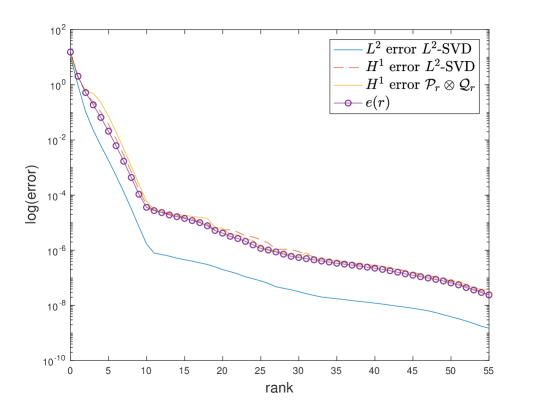
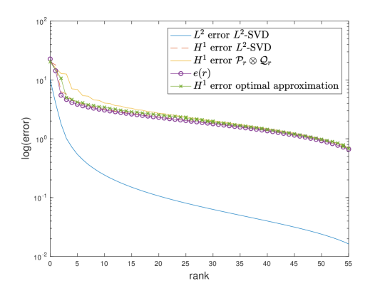
Figure 4.1. Low rank approximations for truncated Fourier series of $u(x,y)=(x^{2}+y^{2})^{0.3}$ (top), $u(x,y)=|x+y|^{0.6}$ (bottom).

These findings suggest that we can compute a low-rank approximation for $u_{n}$ by performing an $L^{2}$-SVD and truncating based on the error estimator in (4.1) to control the error in $H^{1}$. In the following we do just that. We consider the weak formulation of the Poisson equation $-\Delta u=f.$ We compute a Galerkin approximation $u_{n}\approx u$, and truncate this approximation to $\tilde{u}_{n}$ such that

$$\|u-u_{n}\|_{1}\leq\|u-\tilde{u}_{n}\|_{1}\leq 2\|u-u_{n}\|_{1}.$$

We increase the discretization size $n$, i.e., the number $n^{2}$ of basis functions. The results are displayed in 4.2. The plotted errors are approximations to the exact errors $\|u-u_{n}\|_{1}$ and $\|u-\tilde{u}_{n}\|_{1}$. In both cases the error bounds are fulfilled and the rank of $\tilde{u}_{n}$ remains below $5$.

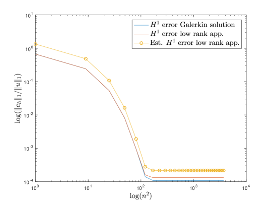
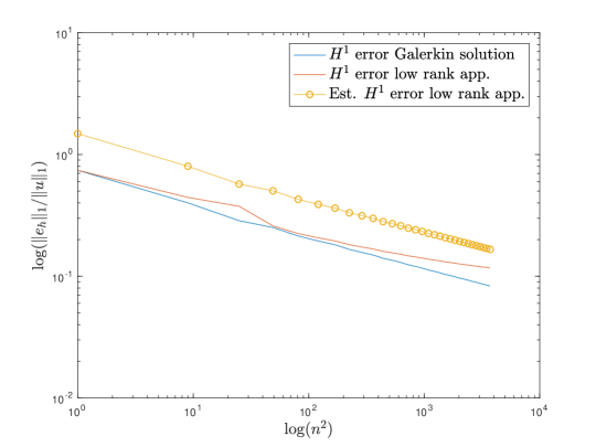
Figure 4.2. Galerkin solutions for reference functions $u(x,y)=\exp(\cos(x)\cos(y))$ (top) and $u(x,y)=|1-(x^{2}+y^{2})|^{0.95}$ (bottom).

5. Conclusion

We proposed and analyzed several variants of low-rank approximations of functions in Sobolev spaces. In part I, we show that sets of functions with bounded Tucker (multi-linear) rank in Sobolev spaces are weakly closed. Sobolev functions can be shown to be in the tensor product of their minimal subspaces under certain conditions, such as additional regularity. However, we do not believe that this holds in general. The $L^{2}$-SVD preserves regularity of the decomposed functions and, under certain conditions, we can quantify the $H^{1}$ error in terms of the rescaled singular values.

In part II, we show that the singular values of different SVDs are closely related. Lower and upper bounds are obtained by simple scalings. We also analyze $H^{1}$ minimal subspaces. The SVD in $H^{(1,0)}$ does not preserve regularity and $H^{1}$ bounds require additional smoothness. The resulting bounds are worse than that of the $L^{2}$-SVD. Similar bounds apply to spaces of lower order mixed smoothness for $d>2$. This indicates the $L^{2}$-SVD performs better for low-rank approximations than variants of SVDs involving Sobolev spaces.

Numerical experiments are consistent with the analytical findings. Differences between minimal subspaces w.r.t. to different norms arise only when considering functions in Sobolev spaces that are not in the algebraic tensor spaces. For constructing low-rank approximations of numerical solutions, the different types of minimal subspaces do not add information. However, the singular values of $H^{(1,0)}$- and $H^{(0,1)}$-SVDs are better suited to estimate the $H^{1}$ error and, for numerical purposes, it seems the best recipe are low-rank approximations built from $L^{2}$-SVDs but with $H^{(1,0)}$ and $H^{(0,1)}$ singular values used for $H^{1}$-error control.

Finally, we briefly mentioned alternatives. Exponential sums are a well known technique already utilized in previous works. On the other hand, if one pursues the viewpoint of Sobolev spaces being intersection spaces, a natural approach would be to consider direct sum spaces. We briefly introduced this viewpoint.

There are a few immediate open questions that arise in conclusion of this work. It would be interesting to consider how the above analysis extends to hierarchical tensor formats (see [5, Chapter 11]). Numerical experiments for high-dimensional problems with a fine or adaptive discretization should shed more light on the performance of SVD in Sobolev spaces.

Appendix A Proof of 3.2

Proof.

I. To begin, we consider the statement for $J=I=(1,\ldots,d)$. We have

$$\|u-\mathcal{P}_{r}u\|_{1}=\left\|\left(\operatorname{id}-\prod_{k=1}^{d}P_{r}^{k}\bigotimes_{i\neq k}\operatorname{id}_{i}\right)u\right\|_{1}=\left\|\sum_{j=1}^{d}\prod_{k=1}^{j-1}P_{r}^{k}\bigotimes_{i\neq k}\operatorname{id}_{i}\left(u-\mathcal{P}_{r}^{j}u\right)\right\|_{1}$$

$$\leq\sum_{j=1}^{d}\left\|\prod_{k=1}^{j-1}P_{r}^{k}\bigotimes_{i\neq k}\operatorname{id}_{i}\left(u-\mathcal{P}_{r}^{j}u\right)\right\|_{1}\leq\sum_{j=1}^{d}\left\|\prod_{k=1}^{j-1}P_{r}^{k}\bigotimes_{i\neq k}\operatorname{id}_{i}\left(u-\mathcal{P}_{r}^{j}u\right)\right\|_{\text{mix},j}$$

$$=\sum_{j=1}^{d}\left\|\left(P_{r}^{1}\otimes\cdots\otimes P_{r}^{j-1}\otimes\operatorname{id}_{j}\otimes\cdots\otimes\operatorname{id}_{d}\right)\left(u-\mathcal{P}_{r}^{j}u\right)\right\|_{\text{mix},j}$$

Thus, we need to bound the norm of the operator

$$P_{r}^{1}\otimes\cdots\otimes P_{r}^{j-1}\otimes\operatorname{id}_{j}\otimes\cdots\otimes\operatorname{id}_{d}:\overline{\mathbb{V}_{j}}^{\|\cdot\|_{\text{mix},j}}\rightarrow\overline{\mathbb{V}_{j}}^{\|\cdot\|_{\text{mix},j}}.$$

Since $\|\cdot\|_{\text{mix},j}$ is a uniform crossnorm on $\overline{\mathbb{V}_{j}}^{\|\cdot\|_{\text{mix},j}}$, we only need to bound

$$P_{r}^{1}\otimes\cdots\otimes P_{r}^{j-1}\otimes\operatorname{id}_{j+1}\otimes\cdots\otimes\operatorname{id}_{d}:H^{1}(\bigtimes_{k\neq j}\Omega_{k})\rightarrow H^{1}(\bigtimes_{k\neq j}\Omega_{k}).$$

II. To that end, we first check if $P_{r}^{j}$ is bounded in $L^{2}$. In order to describe the space $M^{j}_{r}$, we consider again the SVD of the operator $u:H^{1}(\Omega_{j})\rightarrow H^{1}(\bigtimes_{k\neq j}\Omega_{k})$. To shorten notation, we use $x_{j}^{\wedge}:=(x_{1},\ldots,x_{j-1},x_{j+1},\ldots,x_{d})$ and $x_{j}^{\vee}:=(\ldots,x_{j},\ldots)$. We have

$$u[v]=\int_{\Omega_{j}}u(x_{j}^{\vee})v(x_{j})dx_{j}+\int_{\Omega_{j}}\frac{\partial}{\partial x_{j}}u(x_{j}^{\vee})\frac{d}{dx_{j}}v(x_{j})dx_{j},$$

and

$$u^{*}[w]=\int_{\bigtimes_{k\neq j}\Omega_{k}}u(\ldots,x_{j-1},\cdot,x_{j+1},\ldots)w(x_{j}^{\wedge})dx_{j}^{\wedge}$$

$$+\sum_{i\neq j}\int_{\bigtimes_{k\neq j}\Omega_{k}}\frac{\partial}{\partial x_{i}}u(\ldots,x_{j-1},\cdot,x_{j+1},\ldots)\frac{\partial}{\partial x_{i}}v(x_{j}^{\wedge})dx_{j}^{\wedge}.$$

The singular functions $\psi_{k}^{j}\in H^{1}(\Omega_{j})$ satisfy

$$u^{*}u[\psi_{k}]=\int_{\bigtimes_{k\neq j}\Omega_{k}}u(\ldots,x_{j-1},\cdot,x_{j+1},\ldots)\int_{\Omega_{j}}u(x)\psi_{k}^{j}(x_{j})dx_{j}dx_{j}^{\wedge}$$

$$+\int_{\bigtimes_{k\neq j}\Omega_{k}}u(\ldots,x_{j-1},\cdot,x_{j+1},\ldots)\int_{\Omega_{j}}\frac{\partial}{\partial x_{j}}u(x)\frac{d}{dx_{j}}\psi_{k}^{j}(x_{j})dx_{j}dx_{j}^{\wedge}$$

$$+\sum_{i\neq j}\int_{\bigtimes_{k\neq j}\Omega_{k}}\frac{\partial}{\partial x_{i}}u(\ldots,x_{j-1},\cdot,x_{j+1},\ldots)\int_{\Omega_{j}}\frac{\partial}{\partial x_{i}}u(x)\psi_{k}^{j}(x_{j})dx_{j}dx_{j}^{\wedge}$$

$$+\sum_{i\neq j}\int_{\bigtimes_{k\neq j}\Omega_{k}}\frac{\partial}{\partial x_{i}}u(\ldots,x_{j-1},\cdot,x_{j+1},\ldots)\int_{\Omega_{j}}\frac{\partial^{2}}{\partial x_{i}\partial x_{j}}u(x_{j}^{\vee})\frac{d}{dx_{j}}\psi_{k}^{j}(x_{j})dx_{j}dx_{j}^{\wedge}$$

$$=\lambda_{k}^{j}\psi_{k}^{j},$$

where $\lambda_{k}^{j}=(\sigma_{k}^{j})^{2}$. Since $u\in H^{3}(\Omega)$, differentiating twice we get

$$\lambda^{j}_{k}\frac{d^{2}}{dx_{j}^{2}}\psi_{k}=\int_{\bigtimes_{k\neq j}\Omega_{k}}\frac{\partial^{2}}{\partial x_{j}^{2}}u(\ldots,x_{j-1},\cdot,x_{j+1},\ldots)\int_{\Omega_{j}}u(x)\psi_{k}^{j}(x_{j})dx_{j}dx_{j}^{\wedge}$$

$$+\int_{\bigtimes_{k\neq j}\Omega_{k}}\frac{\partial^{2}}{\partial x_{j}^{2}}u(\ldots,x_{j-1},\cdot,x_{j+1},\ldots)\int_{\Omega_{j}}\frac{\partial}{\partial x_{j}}u(x)\frac{d}{dx_{j}}\psi_{k}^{j}(x_{j})dx_{j}dx_{j}^{\wedge}$$

$$+\sum_{i\neq j}\int_{\bigtimes_{k\neq j}\Omega_{k}}\frac{\partial^{3}}{\partial x_{j}^{2}\partial x_{i}}u(\ldots,x_{j-1},\cdot,x_{j+1},\ldots)\int_{\Omega_{j}}\frac{\partial}{\partial x_{i}}u(x)\psi_{k}^{j}(x_{j})dx_{j}dx_{j}^{\wedge}$$

$$+\sum_{i\neq j}\int_{\bigtimes_{k\neq j}\Omega_{k}}\frac{\partial^{3}}{\partial x_{j}^{2}\partial x_{i}}u(\ldots,x_{j-1},\cdot,x_{j+1},\ldots)\int_{\Omega_{j}}\frac{\partial^{2}}{\partial x_{i}\partial x_{j}}u(x_{j}^{\vee})\frac{d}{dx_{j}}\psi_{k}^{j}(x_{j})dx_{j}dx_{j}^{\wedge}.$$

Thus, we can apply 2.4 and conclude

$$\|P_{r}^{j}v\|_{1}\leq\sqrt{2r}D_{j}(r)\|v\|_{0},\quad v\in H^{1}(\Omega_{j}).$$

III. With the above we estimate further

$$\|\left(P_{r}^{1}\otimes\cdots\otimes P_{r}^{j-1}\otimes\operatorname{id}_{j+1}\otimes\cdots\otimes\operatorname{id}_{d}\right)v\|_{1}^{2}$$

$$\leq\sum_{l\neq j}\|\left(P_{r}^{1}\otimes\cdots\otimes P_{r}^{j-1}\otimes\operatorname{id}_{j+1}\otimes\cdots\otimes\operatorname{id}_{d}\right)v\|_{e_{l}}^{2}$$

$$\leq\sum_{l\neq j}\prod_{\begin{subarray}{c}k=1,\ldots,j-1,\\ k\neq l\end{subarray}}\|P_{r}^{k}\|^{2}_{H^{1}\leftarrow L_{2}}\|v\|_{\boldsymbol{l}}^{2}$$

$$\leq 4r^{d-2}\max_{l\neq j}\prod_{\begin{subarray}{c}k=1,\ldots,j-1,\\ k\neq l\end{subarray}}D_{k}(r)^{2}\|v\|_{1}^{2}.$$

IV. The last term in the error is simply $\left\|u-\mathcal{P}_{r}^{j}u\right\|^{2}_{\text{mix},j}=\sum_{k=r+1}^{\infty}(\sigma_{k}^{j})^{2}.$ Since the ordering $J\in S_{d}(I)$ can be chosen arbitrarily, the statement follows. ∎

References

- [1] Ali, M., and Nouy, A. Singular Value Decomposition in Sobolev Spaces: Part I. Z. Anal. Anwend. (2020), to appear.
- [2] Ali, M., and Urban, K. HT-AWGM: A Hierarchical Tucker-Adaptive Wavelet Galerkin Method for High Dimensional Elliptic Problems. ArXiv e-prints (May 2018).
- [3] Bachmayr, M., and Dahmen, W. Adaptive low-rank methods for problems on Sobolev spaces with error control in . ESAIM Math. Model. Numer. Anal. 50, 4 (2016), 1107–1136.
- [4] Bachmayr, M., and Dahmen, W. Adaptive low-rank methods: problems on Sobolev spaces. SIAM J. Numer. Anal. 54, 2 (2016), 744–796.
- [5] Hackbusch, W. Tensor spaces and numerical tensor calculus, vol. 42 of Springer Series in Computational Mathematics. Springer, Heidelberg, 2012.
- [6] Yserentant, H. Regularity and approximability of electronic wave functions, vol. 2000 of Lecture Notes in Mathematics. Springer-Verlag, Berlin, 2010.