Convergence and sample complexity of gradient methods
for the model-free linear quadratic regulator problem

Abstract

Model-free reinforcement learning attempts to find an optimal control action for an unknown dynamical system by directly searching over the parameter space of controllers. The convergence behavior and statistical properties of these approaches are often poorly understood because of the nonconvex nature of the underlying optimization problems and the lack of exact gradient computation. In this paper, we take a step towards demystifying the performance and efficiency of such methods by focusing on the standard infinite-horizon linear quadratic regulator problem for continuous-time systems with unknown state-space parameters. We establish exponential stability for the ordinary differential equation (ODE) that governs the gradient-flow dynamics over the set of stabilizing feedback gains and show that a similar result holds for the gradient descent method that arises from the forward Euler discretization of the corresponding ODE. We also provide theoretical bounds on the convergence rate and sample complexity of the random search method with two-point gradient estimates. We prove that the required simulation time for achieving $\epsilon$-accuracy in the model-free setup and the total number of function evaluations both scale as $\log\,(1/\epsilon)$.

I Introduction

In many emerging applications, control-oriented models are not readily available and classical approaches from optimal control may not be directly applicable. This challenge has led to the emergence of Reinforcement Learning (RL) approaches that often perform well in practice. Examples include learning complex locomotion tasks via neural network dynamics [1] and playing Atari games based on images using deep-RL [2].

RL approaches can be broadly divided into model-based [3, 4] and model-free [5, 6]. While model-based RL uses data to obtain approximations of the underlying dynamics, its model-free counterpart prescribes control actions based on estimated values of a cost function without attempting to form a model. In spite of the empirical success of RL in a variety of domains, our mathematical understanding of it is still in its infancy and there are many open questions surrounding convergence and sample complexity. In this paper, we take a step towards answering such questions with a focus on the infinite-horizon Linear Quadratic Regulator (LQR) for continuous-time systems.

The LQR problem is the cornerstone of control theory. The globally optimal solution can be obtained by solving the Riccati equation and efficient numerical schemes with provable convergence guarantees have been developed [7]. However, computing the optimal solution becomes challenging for large-scale problems, when prior knowledge is not available, or in the presence of structural constraints on the controller. This motivates the use of direct search methods for controller synthesis. Unfortunately, the nonconvex nature of this formulation complicates the analysis of first- and second-order optimization algorithms. To make matters worse, structural constraints on the feedback gain matrix may result in a disjoint search landscape limiting the utility of conventional descent-based methods [8]. Furthermore, in the model-free setting, the exact model (and hence the gradient of the objective function) is unknown so that only zeroth-order methods can be used.

In this paper, we study convergence properties of gradient-based methods for the continuous-time LQR problem. In spite of the lack of convexity, we establish (a) exponential stability of the ODE that governs the gradient-flow dynamics over the set of stabilizing feedback gains; and (b) linear convergence of the gradient descent algorithm with a suitable stepsize. We employ a standard convex reparameterization for the LQR problem [9, 10] to establish the convergence properties of gradient-based methods for the nonconvex formulation. In the model-free setting, we also examine convergence and sample complexity of the random search method [11] that attempts to emulate the behavior of gradient descent via gradient approximations resulting from objective function values. For the two-point gradient estimation setting, we prove linear convergence of the random search method and show that the total number of function evaluations and the simulation time required in our results to achieve $\epsilon$-accuracy are proportional to $\log\,(1/\epsilon)$.

For the discrete-time LQR, global convergence guarantees were recently provided in [12] for gradient decent and the random search method with one-point gradient estimates. The authors established a bound on the sample complexity for reaching the error tolerance $\epsilon$ that requires a number of function evaluations that is at least proportional to $(1/\epsilon^{4})\log\,(1/\epsilon)$. If one has access to the infinite-horizon cost values, the number of function evaluations for the random search method with one-point gradient estimates can be improved to $1/\epsilon^{2}$ [13]. In contrast, we focus on the continuous-time LQR and examine the two-point gradient estimation setting. The use of two-point gradient estimates reduces the required number of function evaluations to $1/\epsilon$ [13]. We significantly improve this result by showing that the required number of function evaluations is proportional to $\log\,(1/\epsilon)$. Similarly, the simulation time required in our results is proportional to $\log\,(1/\epsilon)$; this is in contrast to [12] that requires $\mathrm{poly}\,(1/\epsilon)$ simulation time and [13] that assumes an infinite simulation time. Furthermore, our convergence results hold both in terms of the error in the objective value and the optimization variable (i.e., the feedback gain matrix) whereas [12] and [13] only prove convergence in the objective value. We note that the literature on model-free RL is rapidly expanding and recent extensions to Markovian jump linear systems [14], $\mathcal{H}_{\infty}$ robustness analysis through implicit regularization [15], learning distributed LQ problems [16], and output-feedback LQR [17] have been made.

Our presentation is structured as follows. In Section II, we revisit the LQR problem and present gradient-flow dynamics, gradient descent, and the random search algorithm. In Section III, we highlight the main results of the paper. In Section IV, we utilize convex reparameterization of the LQR problem and establish exponential stability of the resulting gradient-flow dynamics and gradient descent method. In Section V, we extend our analysis to the nonconvex landscape of feedback gains. In Section VI, we quantify the accuracy of two-point gradient estimates and, in Section VII, we discuss convergence and sample complexity of the random search method. In Section VIII, we provide an example to illustrate our theoretical developments and, in Section IX, we offer concluding remarks. Most technical details are relegated to the appendices.

Notation

We use $\mathrm{vec}(M)\in\mathbb{R}^{mn}$ to denote the vectorized form of the matrix $M\in\mathbb{R}^{m\times n}$ obtained by concatenating the columns on top of each other. We use $\|M\|_{F}^{2}=\left\langle M,M\right\rangle$ to denote the Frobenius norm, where $\left\langle X,Y\right\rangle\mathrel{\mathop{:}}=\mathrm{trace}\,(X^{T}Y)$ is the standard matricial inner product. We denote the largest singular value of linear operators and matrices by $\|\cdot\|_{2}$ and the spectral induced norm of linear operators by $\|\cdot\|_{S}$

$$\|{\cal M}\|_{2}\;\mathrel{\mathop{:}}=\;\sup_{M}\dfrac{\|{\cal M}(M)\|_{F}}{\|M\|_{F}},~{}~{}~{}\|{\cal M}\|_{S}\;\mathrel{\mathop{:}}=\;\sup_{M}\dfrac{\|{\cal M}(M)\|_{2}}{\|M\|_{2}}.$$

We denote by $\mathbb{S}^{n}\subset\mathbb{R}^{n\times n}$ the set of symmetric matrices. For $M\in\mathbb{S}^{n}$, $M\succ 0$ means $M$ is positive definite and $\lambda_{\min}(M)$ is the smallest eigenvalue. We use $S^{d-1}\subset\mathbb{R}^{d}$ to denote the unit sphere of dimension $d-1$. We denote the expected value by $\operatorname{\mathbb{E}}[\cdot]$ and probability by $\mathbb{P}(\cdot)$. To compare the asymptotic behavior of $f(\epsilon)$ and $g(\epsilon)$ as $\epsilon$ goes to $0$, we use $f=O(g)$ (or, equivalently, $g=\Omega(f)$) to denote $\limsup_{\epsilon\,\rightarrow\,0}f(\epsilon)/g(\epsilon)<\infty$; $f=\tilde{O}(g)$ to denote $f=O(g\log^{k}\!g)$ for some integer $k$; and $f=o(\epsilon)$ to signify $\lim_{\epsilon\,\rightarrow\,0}f(\epsilon)/\epsilon=0$.

II Problem formulation

The infinite-horizon LQR problem for continuous-time LTI systems is given by

$$\operatorname*{minimize}\limits_{x,\,u} ~{}~{}\operatorname{\mathbb{E}}\left[\,\int_{0}^{\infty}(x^{T}(t)Qx(t)\,+\,u^{T}(t)Ru(t))\,\mathrm{d}t\,\right]$$ (1a)

$$\operatorname*{subject~{}to} ~{}~{}\dot{x}\;=\;Ax\;+\;Bu,~{}~{}x(0)\,\sim\,{\cal D}$$ (1b)

where $x(t)\in\mathbb{R}^{n}$ is the state, $u(t)\in\mathbb{R}^{m}$ is the control input, $A$ and $B$ are constant matrices of appropriate dimensions, $Q$ and $R$ are positive definite matrices, and the expectation is taken over a random initial condition $x(0)$ with distribution ${\cal D}$. For a controllable pair $(A,B)$, the solution to (1) is given by

$$u(t)\;=\;-K^{\star}x(t)\;=\;-R^{-1}B^{T}P^{\star}x(t)$$ (2a)

where $$P^{\star}$$ is the unique positive definite solution to the Algebraic Riccati Equation (ARE)

$$A^{T}P^{\star}\,+\,P^{\star}A\,+\,Q\,-\,P^{\star}BR^{-1}B^{T}P^{\star}\;=\;0.$$ (2b)

When the model is known, the LQR problem and the corresponding ARE can be solved efficiently via a variety of techniques [18, 19, 20, 21]. However, these methods are not directly applicable in the model-free setting, i.e., when the matrices $A$ and $B$ are unknown. Exploiting the linearity of the optimal controller, we can alternatively formulate the LQR problem as a direct search for the optimal linear feedback gain, namely

$$\underset{K}{\operatorname*{minimize}}~{}f(K)$$ (3a)

where

$$f(K)\,\mathrel{\mathop{:}}=\,\left\{\begin{array}[]{ll}\mathrm{trace}\left((Q+K^{T}R\,K)X(K)\right),&K\in\mathcal{S}_{K}\\[0.0pt] \infty,&\text{otherwise.}\end{array}\right.$$ (3d)

Here, the function $$f(K) u=-Kx$$ determines the LQR cost in (1a) associated with the linear state-feedback law ,

$$\mathcal{S}_{K}\;\mathrel{\mathop{:}}=\;\{K\in\mathbb{R}^{m\times n}\,|\,A\,-\,BK\ \text{is Hurwitz}\}$$ (3e)

is the set of stabilizing feedback gains and, for any $K\in\mathcal{S}_{K}$,

$$X(K)\;\mathrel{\mathop{:}}=\;\int_{0}^{\infty}\operatorname{\mathbb{E}}\left[x(t)x^{T}(t)\right]\;=\;\int_{0}^{\infty}\mathrm{e}^{(A\,-\,BK)t}\,\Omega\,\mathrm{e}^{(A\,-\,BK)^{T}t}\,\mathrm{d}t$$ (4a)

is the unique solution to the Lyapunov equation

$$(A\,-\,BK)X\;+\;X(A\,-\,BK)^{T}\,+\;\Omega\;=\;0$$ (4b)

and $\Omega\mathrel{\mathop{:}}=\operatorname{\mathbb{E}}\,[x(0)x^{T}(0)]$. To ensure $f(K)=\infty$ for $K\notin\mathcal{S}_{K}$, we assume $\Omega\succ 0$. This assumption also guarantees $K\in\mathcal{S}_{K}$ if and only if the solution $X$ to (4b) is positive definite.

In problem (3), the matrix $K$ is the optimization variable, and ($A$, $B$, $Q\succ 0$, $R\succ 0$, $\Omega\succ 0$) are the problem parameters. This alternative formulation of the LQR problem has been studied for both continuous-time [7] and discrete-time systems [12, 22] and it serves as a building block for several important control problems including optimal static-output feedback design [23], optimal design of sparse feedback gain matrices [24, 25, 26, 27], and optimal sensor/actuator selection [28, 29, 30].

For all stabilizing feedback gains $K\in\mathcal{S}_{K}$, the gradient of the objective function is determined by [23, 24]

$$\nabla f(K)\;=\;2(R\,K\,-\,B^{T}P(K))X(K).$$ (5)

Here, $X(K)$ is given by (4a) and

$$P(K)=\int_{0}^{\infty}\mathrm{e}^{(A\,-\,BK)^{T}t}\,(Q+K^{T}R\,K)\,\mathrm{e}^{(A\,-\,BK)t}\,\mathrm{d}t$$ (6a)

is the unique positive definite solution of

$$(A\,-\,BK)^{T}P\,+\,P(A\,-\,BK)\,=\,-Q\,-\,K^{T}R\,K.$$ (6b)

To simplify our presentation, for any $K\in\mathbb{R}^{m\times n}$, we define the closed-loop Lyapunov operator ${\cal A}_{K}$: $\mathbb{S}^{n}\rightarrow\mathbb{S}^{n}$ as

$${\cal A}_{K}(X) \;\mathrel{\mathop{:}}=\;(A\,-\,BK)X\,+\,X(A\,-\,BK)^{T}.$$ (7a)

For $$K\in\mathcal{S}_{K} {\cal A}_{K}$$, both and its adjoint

$${\cal A}_{K}^{*}(P) \;=\;(A\,-\,BK)^{T}P\,+\,P(A\,-\,BK)$$ (7b)

are invertible and $X(K)$, $P(K)$ are determined by

$$X(K)\,=\,-{\cal A}_{K}^{-1}(\Omega),~{}~{}~{}P(K)\,=\,-({\cal A}_{K}^{*})^{-1}(Q\,+\,K^{T}RK).$$

In this paper, we first examine the global stability properties of the gradient-flow dynamics

$$\dot{K}\;=\;-\nabla f(K),~{}~{}K(0)\,\in\,\mathcal{S}_{K}$$ (GF)

associated with problem (3) and its discretized variant,

$$K^{k+1}\;\mathrel{\mathop{:}}=\;K^{k}\,-\,\alpha\,\nabla f(K^{k}),~{}~{}K^{0}\,\in\,\mathcal{S}_{K}$$ (GD)

where $\alpha>0$ is the stepsize. Next, we use this analysis as a building block to study the convergence of a search method based on random sampling [11, 31] for solving problem (3). As described in Algorithm 1, at each iteration we form an empirical approximation $\macc@depth\char 1\relax\frozen@everymath{\macc@group}\macc@set@skewchar\macc@nested@a 111{\nabla}f(K)$ to the gradient of the objective function via simulation of system (1b) for randomly perturbed feedback gains $K\pm U_{i}$, $i=1,\ldots,N$, and update $K$ via,

$$K^{k+1}\;\mathrel{\mathop{:}}=\;K^{k}\,-\,\alpha\,\macc@depth\char 1\relax\frozen@everymath{\macc@group}\macc@set@skewchar\macc@nested@a 111{\nabla}f(K^{k}),\quad K^{0}\,\in\,\mathcal{S}_{K}.$$ (RS)

We note that the gradient estimation scheme in Algorithm 1 does not require knowledge of system matrices $A$ and $B$ in (1b) but only access to a simulation engine.

Algorithm 1 Two-point gradient estimation

0:  Feedback gain $K\in\mathbb{R}^{m\times n}$, state and control weight matrices $Q$ and $R$, distribution ${\cal D}$, smoothing constant $r$, simulation time $\tau$, number of random samples $N$.

  for $i\,=\,1,\ldots,N$ do

     – Define perturbed feedback gains $K_{i,1}\mathrel{\mathop{:}}=K+rU_{i}$ and $K_{i,2}\mathrel{\mathop{:}}=K-rU_{i}$, where $\mathrm{vec}({U_{i}})$ is a random vector uniformly distributed on the sphere $\sqrt{mn}\,S^{mn-1}$.

     – Sample an initial condition $x_{i}$ from distribution ${\cal D}$.

     – For $j\in\{1,2\}$, simulate system (1b) up to time $\tau$ with the feedback gain $K_{i,j}$ and initial condition $x_{i}$ to form $\displaystyle\hat{f}_{i,j}\,=\,\displaystyle{\int_{0}^{\tau}(x^{T}(t)Qx(t)\,+\,u^{T}(t)Ru(t))\,\mathrm{d}t}$.

  end for

  The gradient estimate $\displaystyle\macc@depth\char 1\relax\frozen@everymath{\macc@group}\macc@set@skewchar\macc@nested@a 111{\nabla}f(K)\,=\,\dfrac{1}{2rN}\,\sum_{i\,=\,1}^{N}\left(\hat{f}_{i,1}\,-\,\hat{f}_{i,2}\right)U_{i}$.

III Main results

Optimization problem (3) is not convex [8]; see Appendix -A for an example. The function $f(K)$, however, has two important properties: uniqueness of the critical points and the compactness of sublevel sets [32, 33]. Based on these, the LQR objective error $f(K)-f(K^{\star})$ can be used as a maximal Lyapunov function (see [34] for a definition) to prove asymptotic stability of gradient-flow dynamics (GF) over the set of stabilizing feedback gains $\mathcal{S}_{K}$. However, this approach does not provide any guarantee on the rate of convergence and additional analysis is necessary to establish exponential stability; see Section V for details.

III-A Known model

We first summarize our results for the case when the model is known. In spite of the nonconvex optimization landscape, we establish the exponential stability of gradient-flow dynamics (GF) for any stabilizing initial feedback gain $K(0)$. This result also provides an explicit bound on the rate of convergence to the LQR solution $K^{\star}$.

Theorem 1

For any initial stabilizing feedback gain $K(0)\in\mathcal{S}_{K}$, the solution $K(t)$ to gradient-flow dynamics (GF) satisfies

$$f(K(t))\,-\,f(K^{\star}) \;\leq\;\mathrm{e}^{-\rho\,t}\left(f(K(0))\,-\,f(K^{\star})\right)$$

$$\|K(t)\,-\,K^{\star}\|^{2}_{F} \;\leq\;b\,\mathrm{e}^{-\rho\,t}\,\|K(0)\,-\,K^{\star}\|_{F}^{2}$$

where the convergence rate $\rho$ and constant $b$ depend on $K(0)$ and the parameters of the LQR problem (3).

The proof of Theorem 1 along with explicit expressions for the convergence rate $\rho$ and constant $b$ are provided in Section V-A. Moreover, for a sufficiently small stepsize $\alpha$, we show that gradient descent method (GD) also converges over $\mathcal{S}_{K}$ at a linear rate.

Theorem 2

For any initial stabilizing feedback gain $K^{0}\in\mathcal{S}_{K}$, the iterates of gradient descent (GD) satisfy

$$f(K^{k})\,-\,f(K^{\star}) \;\leq\;\gamma^{k}\left(f(K^{0})\,-\,f(K^{\star})\right)$$

$$\|K^{k}\,-\,K^{\star}\|^{2}_{F} \;\leq\;b\,\gamma^{k}\,\|K^{0}\,-\,K^{\star}\|_{F}^{2}$$

where the rate of convergence $\gamma$, stepsize $\alpha$, and constant $b$ depend on $K^{0}$ and the parameters of the LQR problem (3).

III-B Unknown model

We now turn our attention to the model-free setting. We use Theorem 2 to carry out the convergence analysis of the random search method (RS) under the following assumption on the distribution of initial condition.

Assumption 1

Let the distribution $\mathcal{D}$ of the initial conditions have i.i.d. zero-mean unit-variance entries with bounded sub-Gaussian norm, i.e., for a random vector $v\in\mathbb{R}^{n}$ distributed according to $\mathcal{D}$, $\mathbb{E}[v_{i}]=0$ and $\|v_{i}\|_{\psi_{2}}\leq\kappa$, for some constant $\kappa$ and $i=1,\ldots,n$; see Appendix -J for the definition of $\|\cdot\|_{\psi_{2}}$.

Our main convergence result holds under Assumption 1. Specifically, for a desired accuracy level $\epsilon>0$, in Theorem 3 we establish that iterates of (RS) with constant stepsize (that does not depend on $\epsilon$) reach accuracy level $\epsilon$ at a linear rate (i.e., in at most $O(\log\,(1/\epsilon))$ iterations) with high probability. Furthermore, the total number of function evaluations and the simulation time required to achieve an accuracy level $\epsilon$ are proportional to $\log\,(1/\epsilon)$. This significantly improves the existing results for discrete-time LQR [12, 13] that require $O(1/\epsilon)$ function evaluations and $\mathrm{poly}(1/\epsilon)$ simulation time.

Theorem 3 (Informal)

Let the initial condition $x_{0}\sim{\cal D}$ of system (1b) obey Assumption 1. Also let the simulation time $\tau$ and the number of samples $N$ in Algorithm 1 satisfy

$$\tau\,\geq\,\theta_{1}\log\,(1/\epsilon)~{}\text{and}~{}N\,\geq\,c\left(1\,+\,\beta^{4}\kappa^{4}\,\theta_{1}\log^{6}\!n\right)n$$

for some $\beta>0$ and desired accuracy $\epsilon>0$. Then, we can choose the smoothing parameter $r<\theta_{3}\sqrt{\epsilon}$ in Algorithm 1 and the constant stepsize $\alpha$ such that the random search method (RS) that starts from any initial stabilizing feedback gain $K^{0}\in\mathcal{S}_{K}$ achieves $f(K^{k})-f(K^{\star})\leq\epsilon$ in at most

$$k\;\leq\;\theta_{4}\log\left((f(K^{0})\,-\,f(K^{\star}))/\epsilon\right)$$

iterations with probability not smaller than $1-c^{\prime}k(n^{-\beta}+N^{-\beta}+N\mathrm{e}^{-\frac{n}{8}}+\mathrm{e}^{-c^{\prime}N})$. Here, the positive scalars $c$ and $c^{\prime}$ are absolute constants and $\theta_{1},\ldots,\theta_{4}>0$ depend on $K^{0}$ and the parameters of the LQR problem (3).

The formal version of Theorem 3 along with a discussion of parameters $\theta_{i}$ and stepsize $\alpha$ is presented in Section VII.

IV Convex reparameterization

The main challenge in establishing the exponential stability of (GF) arises from nonconvexity of problem (3). Herein, we use a standard change of variables to reparameterize (3) into a convex problem, for which we can provide exponential stability guarantees for gradient-flow dynamics. We then connect the gradient flow on this convex reparameterization to its nonconvex counterpart and establish the exponential stability of (GF).

IV-A Change of variables

The stability of the closed-loop system with the feedback gain $K\in\mathcal{S}_{K}$ in problem (3) is equivalent to the positive definiteness of the matrix $X(K)$ given by (4a). This condition allows for a standard change of variables $K=YX^{-1}$, for some $Y\in\mathbb{R}^{m\times n}$, to reformulate the LQR design as a convex optimization problem [9, 10]. In particular, for any $K\in\mathcal{S}_{K}$ and the corresponding matrix $X$, we have

$$f(K)\;=\;h(X,Y)\;\mathrel{\mathop{:}}=\;\mathrm{trace}\,(Q\,X+Y^{T}R\,YX^{-1})$$

where $h(X,Y)$ is a jointly convex function of $(X,Y)$ for $X\succ 0$. In the new variables, Lyapunov equation (4b) takes the affine form

$${\cal A}(X)\;-\;{\cal B}(Y)\;+\;\Omega\;=\;0$$ (8a)

where $${\cal A} {\cal B}$$ and are the linear maps

$${\cal A}(X)\,\mathrel{\mathop{:}}=\,A\,X\,+\,XA^{T},~{}~{}~{}{\cal B}(Y)\,\mathrel{\mathop{:}}=\,B\,Y\,+\,Y^{T}B^{T}.$$ (8b)

For an invertible map $${\cal A} X Y$$, we can express the matrix as an affine function of

$$X(Y)\,=\,{\cal A}^{-1}({\cal B}(Y)\,-\,\Omega)$$ (8c)

and bring the LQR problem into the convex form

$$\underset{Y}{\operatorname*{minimize}}\quad h(Y)$$ (9)

where

$$h(Y)\;\mathrel{\mathop{:}}=\;\left\{\begin{array}[]{ll}h(X(Y),Y),&Y\,\in\,\mathcal{S}_{Y}\\[0.0pt] \infty,&\text{otherwise}\end{array}\right.$$

and $\mathcal{S}_{Y}\mathrel{\mathop{:}}=\{Y\in\mathbb{R}^{m\times n}\,|\,X(Y)\succ 0\}$ is the set of matrices $Y$ that correspond to stabilizing feedback gains $K=YX^{-1}$. The set $\mathcal{S}_{Y}$ is open and convex because it is defined via a positive definite condition imposed on the affine map $X(Y)$ in (8c). This positive definite condition in $\mathcal{S}_{Y}$ is equivalent to the closed-loop matrix $A-B\,Y(X(Y))^{-1}$ being Hurwitz.

Remark 1

Although our presentation assumes invertibility of ${\cal A}$, this assumption comes without loss of generality. As shown in Appendix -B, all results carry over to noninvertible ${\cal A}$ with an alternative change of variables $A=\hat{A}+BK^{0}$, $K=\hat{K}+K^{0}$, and $\hat{K}=\hat{Y}X^{-1}$, for some $K^{0}\in\mathcal{S}_{K}$.

IV-B Smoothness and strong convexity of $h(Y)$

Our convergence analysis of gradient methods for problem (8) relies on the $L$-smoothness and $\mu$-strong convexity of the function $h(Y)$ over its sublevel sets $\mathcal{S}_{Y}(a)\mathrel{\mathop{:}}=\{Y\in\mathcal{S}_{Y}\,|\,h(Y)\leq a\}.$ These two properties were recently established in [30] where it was shown that over any sublevel set $\mathcal{S}_{Y}(a)$, the second-order term $\left\langle\tilde{Y},\nabla^{2}h(Y;\tilde{Y})\right\rangle$ in the Taylor series expansion of $h(Y+\tilde{Y})$ around $Y\in\mathcal{S}_{Y}(a)$ can be upper and lower bounded by quadratic forms $L\|\tilde{Y}\|_{F}^{2}$ and $\mu\|\tilde{Y}\|_{F}^{2}$ for some positive scalars $L$ and $\mu$. While an explicit form for the smoothness parameter $L$ along with an existence proof for the strong convexity modulus $\mu$ were presented in [30], in Proposition 1 we establish an explicit expression for $\mu$ in terms of $a$ and parameters of the LQR problem. This allows us to provide bounds on the convergence rate for gradient methods.

Proposition 1

Over any non-empty sublevel set $\mathcal{S}_{Y}(a)$, the function $h(Y)$ is $L$-smooth and $\mu$-strongly convex with

$$L \;=\;\dfrac{2a\|R\|_{2}}{\nu}\left(1\,+\,\dfrac{a\|{\cal A}^{-1}{\cal B}\|_{2}}{\sqrt{\nu\lambda_{\min}(R)}}\right)^{2}$$ (10a)

$$\mu \;=\;\dfrac{2\lambda_{\min}(R)\lambda_{\min}(Q)}{a\left(1\,+\,a^{2}\eta\right)^{2}}$$ (10b)

where the constants

$$\eta \;\mathrel{\mathop{:}}=\;\dfrac{\|{\cal B}\|_{2}}{\lambda_{\min}(Q)\lambda_{\min}(\Omega)\sqrt{\nu\,\lambda_{\min}(R)}}$$ (10c)

$$\nu \;\mathrel{\mathop{:}}=\;\dfrac{\lambda_{\min}^{2}(\Omega)}{4}\left(\dfrac{\|A\|_{2}}{\sqrt{\lambda_{\min}(Q)}}\,+\,\dfrac{\|B\|_{2}}{\sqrt{\lambda_{\min}(R)}}\right)^{-2}$$ (10d)

only depend on the problem parameters.

Proof:

See Appendix -C. ∎

IV-C Gradient methods over $\mathcal{S}_{Y}$

The LQR problem can be solved by minimizing the convex function $h(Y)$ whose gradient is given by [30, Appendix C]

$$\nabla h(Y)\;=\;2\,R\,Y(X(Y))^{-1}\,-\,2\,B^{T}W(Y)$$ (11a)

where $$W(Y)$$ is the solution to

$$A^{T}\,W\,+\,WA\;=\;(X(Y))^{-1}\,Y^{T}R\,Y(X(Y))^{-1}\,-\,Q.$$ (11b)

Using the strong convexity and smoothness properties of $h(Y)$ established in Proposition 1, we next show that the unique minimizer $Y^{\star}$ of the function $h(Y)$ is the exponentially stable equilibrium point of the gradient-flow dynamics over $\mathcal{S}_{Y}$,

$$\dot{Y}\;=\;-\nabla h(Y),\quad Y(0)\,\in\,\mathcal{S}_{Y}.$$ (GFY)

Proposition 2

For any $Y(0)\in\mathcal{S}_{Y}$, the gradient-flow dynamics (GFY) are exponentially stable, i.e.,

$$\|Y(t)\,-\,Y^{\star}\|_{F}^{2}\;\leq\;(L/\mu)\,\mathrm{e}^{-2\,\mu\,t}\,\|Y(0)\,-\,Y^{\star}\|_{F}^{2}$$

where $\mu$ and $L$ are the strong convexity and smoothness parameters of the function $h(Y)$ over the sublevel set $\mathcal{S}_{Y}(h(Y(0)))$.

Proof:

The derivative of the Lyapunov function candidate $V(Y)\mathrel{\mathop{:}}=h(Y)-h(Y^{\star})$ along the flow in (GFY) satisfies

$$\dot{V}\;=\;\left\langle\nabla h(Y),\dot{Y}\right\rangle\;=\;-\|\nabla h(Y)\|_{F}^{2}\;\leq\;-2\,\mu V.$$ (12)

Inequality (12) is a consequence of the strong convexity of $h(Y)$ and it yields [35, Lemma 3.4]

$$V(Y(t))\;\leq\;\mathrm{e}^{-2\,\mu\,t}\,V(Y(0)).$$ (13)

Thus, for any $Y(0)\in\mathcal{S}_{Y}$, $h(Y(t))$ converges exponentially to $h(Y^{\star})$. Moreover, since $h(Y)$ is $\mu$-strongly convex and $L$-smooth, $V(Y)$ can be upper and lower bounded by quadratic functions and the exponential stability of (GFY) over $\mathcal{S}_{Y}$ follows from Lyapunov theory [35, Theorem 4.10]. ∎

In Section V, we use the above result to prove exponential/linear convergence of gradient flow/descent for the nonconvex optimization problem (3). Before we proceed, we note that similar convergence guarantees can be established for the gradient descent method with a sufficiently small stepsize $\alpha$,

$$Y^{k+1}\;\mathrel{\mathop{:}}=\;Y^{k}\;-\;\alpha\,\nabla h(Y^{k}),\quad Y^{0}\,\in\,\mathcal{S}_{Y}$$ (GY)

Since the function $h(Y)$ is $L$-smooth over the sublevel set $\mathcal{S}_{Y}(h(Y^{0}))$, for any $\alpha\in[0,1/L]$ the iterates $Y^{k}$ remain within $\mathcal{S}_{Y}(h(Y^{0}))$. This property in conjunction with the $\mu$-strong convexity of $h(Y)$ imply that $Y^{k}$ converges to the optimal solution $Y^{\star}$ at a linear rate of $\gamma=1-\alpha\mu$.

V Control design with a known model

The asymptotic stability of (GF) is a consequence of the following properties of the LQR objective function [32, 33]:

1. The function $f(K)$ is twice continuously differentiable over its open domain $\mathcal{S}_{K}$ and $f(K)\rightarrow\infty$ as $K\rightarrow\infty$ and/or $K\rightarrow\partial\mathcal{S}_{K}$.

2. The optimal solution $K^{\star}$ is the unique equilibrium point over ${\cal S}_{K}$, i.e., $\nabla f(K)=0$ if and only if $K=K^{\star}$.

In particular, the derivative of the maximal Lyapunov function candidate $V(K)\mathrel{\mathop{:}}=f(K)-f(K^{\star})$ along the trajectories of (GF) satisfies

$$\dot{V}\;=\;\left\langle\nabla f(K),\dot{K}\right\rangle\;=\;-\|\nabla f(K)\|_{F}^{2}\;\leq\;0$$

where the inequality is strict for all $K\neq K^{\star}$. Thus, Lyapunov theory [34] implies that, starting from any stabilizing initial condition $K(0)$, the trajectories of (GF) remain within the sublevel set $\mathcal{S}_{K}(f(K(0)))$ and asymptotically converge to $K^{\star}$.

Similar arguments were employed for the convergence analysis of the Anderson-Moore algorithm for output-feedback synthesis [32]. While [32] shows global asymptotic stability, it does not provide any information on the rate of convergence. In this section, we first demonstrate exponential stability of (GF) and prove Theorem 1. Then, we establish linear convergence of the gradient descent method (GD) and prove Theorem 2.

V-A Gradient-flow dynamics: proof of Theorem 1

We start our proof of Theorem 1 by relating the convex and nonconvex formulations of the LQR objective function. Specifically, in Lemma 1, we establish a relation between the gradients $\nabla f(K)$ and $\nabla h(Y)$ over the sublevel sets of the objective function $\mathcal{S}_{K}(a)\mathrel{\mathop{:}}=\{K\in\mathcal{S}_{K}\,|\,f(K)\leq a\}.$

Lemma 1

For any stabilizing feedback gain $K\in\mathcal{S}_{K}(a)$ and $Y\mathrel{\mathop{:}}=KX(K)$, we have

$$\|\nabla f(K)\|_{F} \;\geq\;c\,\|\nabla h(Y)\|_{F}$$ (14a)

where $$X(K) c$$ is given by (4a), the constant is determined by

$$c \;=\;\dfrac{\nu\sqrt{\nu\,\lambda_{\min}(R)}}{2\,a^{2}\,\|{\cal A}^{-1}\|_{2}\,\|B\|_{2}\,+\,a\,\sqrt{\nu\,\lambda_{\min}(R)}}$$ (14b)

and the scalar $\nu$ given by Eq. (10d) depends on the problem parameters.

Proof:

See Appendix -D. ∎

Using Lemma 1 and the exponential stability of gradient-flow dynamics (GFY) over $\mathcal{S}_{Y}$, established in Proposition 2, we next show that (GF) is also exponentially stable. In particular, for any stabilizing $K\in\mathcal{S}_{K}(a)$, the derivative of $V(K)\mathrel{\mathop{:}}=f(K)-f(K^{\star})$ along the gradient flow in (GF) satisfies

$$\dot{V}\;=\,-\|\nabla f(K)\|_{F}^{2}\;\leq\,-c^{2}\,\|\nabla h(Y)\|_{F}^{2}\;\leq\,-2\,\mu\,c^{2}\,V$$ (15)

where $Y=KX(K)$ and the constants $c$ and $\mu$ are provided in Lemma 1 and Proposition 1, respectively. The first inequality in (15) follows from (14a) and the second follows from $f(K)=h(Y)$ combined with $\|\nabla h(Y)\|_{F}^{2}\geq 2\mu V$ (which in turn is a consequence of the strong convexity of $h(Y)$ established in Proposition 1).

Now, since the sublevel set $\mathcal{S}_{K}(a)$ is invariant with respect to (GF), following [35, Lemma 3.4], inequality (15) guarantees that system (GF) converges exponentially in the objective value with rate $\rho=2\mu c^{2}.$ This concludes the proof of part (a) in Theorem 1. In order to prove part (b), we use the following lemma which connects the errors in the objective value and the optimization variable.

Lemma 2

For any stabilizing feedback gain $K$, the objective function $f(K)$ in problem (3) satisfies

$$f(K)\,-\,f(K^{\star})\;=\;\mathrm{trace}\left((K-K^{\star})^{T}R\,(K-K^{\star})\,X(K)\right)$$

where $K^{\star}$ is the optimal solution and $X(K)$ is given by (4a).

Proof:

See Appendix -D. ∎

From Lemma 2 and part (a) of Theorem 1, we have

$$\begin{array}[]{rcl}\|K(t)\,-\,K^{\star}\|^{2}_{F}&\!\!\!\leq\!\!\!&\dfrac{f(K(t))\,-\,f(K^{\star})}{\lambda_{\min}(R)\,\lambda_{\min}(X(K(t)))}\;\leq\;\mathrm{e}^{-\rho\,t}\,\dfrac{f(K(0))\,-\,f(K^{\star})}{\lambda_{\min}(R)\,\lambda_{\min}(X(K(t)))}\;\leq\;b^{\prime}\,\mathrm{e}^{-\rho\,t}\,\|K(0)\,-\,K^{\star}\|^{2}_{F}\end{array}$$

where $b^{\prime}\mathrel{\mathop{:}}={\|R\|_{2}\|X(K(0))\|_{2}}/(\lambda_{\min}(R)\lambda_{\min}(X(K(t)))).$ Here, the first and third inequalities follow form basic properties of the matrix trace combined with Lemma 2 applied with $K=K(t)$ and $K=K(0)$, respectively. The second inequality follows from part (a) of Theorem 1.

Finally, to upper bound parameter $b^{\prime}$, we use Lemma 23 presented in Appendix -K that provides the lower and upper bounds ${\nu}/{a}\leq\lambda_{\min}(X(K))$ and $\|X(K)\|_{2}\leq a/\lambda_{\min}(Q)$ on the matrix $X(K)$ for any $K\in\mathcal{S}_{K}(a)$, where the constant $\nu$ is given by (10d). Using these bounds and the invariance of $\mathcal{S}_{K}(a)$ with respect to (GF), we obtain

$$b^{\prime}\;\leq\;b\;\mathrel{\mathop{:}}=\;\dfrac{a^{2}\,\|R\|_{2}}{\nu\,\lambda_{\min}(R)\,\lambda_{\min}(Q)}$$ (16)

which completes the proof of part (b).

Remark 2 (Gradient domination)

Expression (15) implies that the objective function $f(K)$ over any given sublevel set $\mathcal{S}_{K}(a)$ satisfies the Polyak-Łojasiewicz (PL) condition [36]

$$\|\nabla f(K)\|_{F}^{2}\;\geq\;{2\,\mu_{f}}\left(f(K)\,-\,f(K^{\star})\right)$$ (17)

with parameter $\mu_{f}\mathrel{\mathop{:}}=\mu\,c^{2}$, where $\mu$ and $c$ are functions of $a$ that are given by (10b) and (14b), respectively. This condition is also known as gradient dominance and it was recently used to show convergence of gradient-based methods for discrete-time LQR problem [12].

V-B Geometric interpretation

The solution $Y(t)$ to gradient-flow dynamics (GFY) over the set $\mathcal{S}_{Y}$ induces the trajectory

$$K_{\mathrm{ind}}(t)\;\mathrel{\mathop{:}}=\;Y(t)(X(Y(t)))^{-1}$$ (18)

over the set of stabilizing feedback gains $\mathcal{S}_{K}$, where the affine function $X(Y)$ is given by (8c). The induced trajectory $K_{\mathrm{ind}}(t)$ can be viewed as the solution to the differential equation

$$\dot{K}\;=\;g(K)$$ (19a)

where $$g \mathcal{S}_{K}\rightarrow\mathbb{R}^{m\times n}$$: is given by

$$g(K)\,\mathrel{\mathop{:}}=\,\left(K{\cal A}^{-1}({\cal B}(\nabla h(Y(K))))-\nabla h(Y(K))\right)(X(K))^{-1}.$$ (19b)

Here, the matrix $X=X(K)$ is given by (4a) and $Y(K)=KX(K)$. System (19) is obtained by differentiating both sides of Eq. (18) with respect to time $t$ and applying the chain rule. Figure 1 illustrates an induced trajectory $K_{\mathrm{ind}}(t)$ and a trajectory $K(t)$ resulting from gradient-flow dynamics (GF) that starts from the same initial condition.

Moreover, using the definition of $h(Y)$, we have

$$h(Y(t))\;=\;f(K_{\mathrm{ind}}(t)).$$ (20)

Thus, the exponential decay of $h(Y(t))$ established in Proposition 2 implies that $f$ decays exponentially along the vector field $g$, i.e., for $K_{\mathrm{ind}}(0)\neq K^{\star}$, we have

$$\dfrac{f(K_{\mathrm{ind}}(t))\,-\,f(K^{\star})}{f(K_{\mathrm{ind}}(0))\,-\,f(K^{\star})}\;=\;\dfrac{h(Y(t))\,-\,h(Y^{\star})}{h(Y(0))\,-\,h(Y^{\star})}\;\leq\;\mathrm{e}^{-2\,\mu\,t}.$$

This inequality follows from inequality (13), where $\mu$ denotes the strong-convexity modulus of the function $h(Y)$ over the sublevel set $\mathcal{S}_{Y}(h(Y(0)))$; see Proposition 1. Herein, we provide a geometric interpretation of the exponential decay of $f$ under the trajectories of (GF) that is based on the relation between the vector fields $g$ and $-\nabla f$.

Differentiating both sides of Eq. (20) with respect to $t$ yields

$$\|\nabla h(Y)\|^{2}=\left\langle-\nabla f(K),g(K)\right\rangle.$$ (21)

Thus, for each $K\in\mathcal{S}_{K}$, the inner product between the vector fields $-\nabla f(K)$ and $g(K)$ is nonnegative. However, this is not sufficient to ensure exponential decay of $f$ along (GF). To address this challenge, our proof utilizes inequality (14a) in Lemma 1. Based on (21), (14a) can be equivalently restated as

$$\dfrac{\|-\nabla f(K)\|_{F}}{\|\mathrm{\Pi}_{-\nabla f(K)}(g(K))\|_{F}}\;=\;\dfrac{\|\nabla f(K)\|_{F}^{2}}{\left\langle-\nabla f(K),g(K)\right\rangle}\;\geq\;c^{2}$$

where $\Pi_{b}(a)$ denotes the projection of $a$ onto $b$. Thus, Lemma 1 ensures that the ratio between the norm of the vector field $-\nabla f(K)$ associated with gradient-flow dynamics (GF) and the norm of the projection of $g(K)$ onto $-\nabla f(K)$ is uniformly lower bounded by a positive constant. This lower bound is the key geometric feature that allows us to deduce exponential decay of $f$ along the vector field $-\nabla f$ from the exponential decay of the vector field $g$.

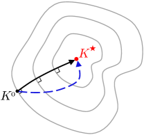
Figure 1: Trajectories $K(t)$ of (GF) (solid black) and $K_{\mathrm{ind}}(t)$ resulting from Eq. (18) (dashed blue) along with the level sets of the function $f(K)$.

V-C Gradient descent: proof of Theorem 2

Given the exponential stability of gradient-flow dynamics (GF) established in Theorem 1, the convergence analysis of gradient descent (GD) amounts to finding a suitable stepsize $\alpha$. Lemma 3 provides a Lipschitz continuity parameter for $\nabla f(K)$, which facilitates finding such a stepsize.

Lemma 3

Over any non-empty sublevel set $\mathcal{S}_{K}(a)$, the gradient $\nabla f(K)$ is Lipschitz continuous with parameter

$$L_{f}\;\mathrel{\mathop{:}}=\;\dfrac{2a\|R\|_{2}}{\lambda_{\min}(Q)}\,+\,\dfrac{8a^{3}\|B\|_{2}}{\lambda_{\min}^{2}(Q)\lambda_{\min}(\Omega)}\big{(}\dfrac{\|B\|_{2}}{\lambda_{\min}(\Omega)}\,+\,\dfrac{\|R\|_{2}}{\sqrt{\nu\lambda_{\min}(R)}}\!\big{)}$$

where $\nu$ given by (10d) depends on the problem parameters.

Proof:

See Appendix -D. ∎

Let $K_{\alpha}\mathrel{\mathop{:}}=K-\alpha\,\nabla f(K)$, $\alpha\geq 0$ parameterize the half-line starting from $K\in\mathcal{S}_{K}(a)$ with $K\neq K^{\star}$ along $-\nabla f(K)$ and let us define the scalar $\beta_{m}\mathrel{\mathop{:}}=\max\beta$ such that $K_{\alpha}\in\mathcal{S}_{K}(a)$, for all $\alpha\in[0,\beta]$. The existence of $\beta_{m}$ follows from the compactness of $\mathcal{S}_{K}(a)$ [32]. We next show that $\beta_{m}\geq 2/L_{f}$.

For the sake of contradiction, suppose $\beta_{m}<2/L_{f}$. From the continuity of $f(K_{\alpha})$ with respect to $\alpha$, it follows that $f(K_{\beta_{s}})=a$. Moreover, since $-\nabla f(K)$ is a descent direction of the function $f(K)$, we have $\beta_{m}>0$. Thus, for $\alpha\in(0,\beta_{m}]$,

$$f(K_{\alpha})\,-\,f(K)\;\leq\;-\dfrac{\alpha(2\,-\,L_{f}\alpha)}{2}\,\|\nabla f(K)\|_{F}^{2}\;<\;0.$$

Here, the first inequality follows from the $L_{f}$-smoothness of $f(K)$ over $\mathcal{S}_{K}(a)$ (Descent Lemma [37, Eq. (9.17)]) and the second inequality follows from $\nabla f(K)\neq 0$ in conjunction with $\beta_{m}\in(0,2/L_{f})$. This implies $f(K_{\beta_{m}})<f(K)\leq a$, which contradicts $f(K_{\beta_{m}})=a$. Thus, $\beta_{m}\geq 2/L_{f}$.

We can now use induction on $k$ to show that, for any stabilizing initial condition $K^{0}\in\mathcal{S}_{K}(a)$, the iterates of (GD) with $\alpha\in[0,2/L_{f}]$ remain in $\mathcal{S}_{K}(a)$ and satisfy

$$f(K^{k+1})\,-\,f(K^{k})\;\leq\;-\dfrac{\alpha(2\,-\,L_{f}\alpha)}{2}\,\|\nabla f(K^{k})\|_{F}^{2}.$$ (22)

Inequality (22) in conjunctions with the PL condition (17) evaluated at $K^{k}$ guarantee linear convergence for gradient descent (GD) with the rate $\gamma\leq 1-\alpha\,\mu_{f}$ for all $\alpha\in(0,1/L_{f}]$, where $\mu_{f}$ is the PL parameter of the function $f(K)$. This completes the proof of part (a) of Theorem 2.

Using part (a) and Lemma 2, we can make a similar argument to what we used for the proof of Theorem 1 to establish part (b) with constant $b$ in (16). We omit the details for brevity.

Remark 3

Using our results, it is straightforward to show linear convergence of $K^{k+1}=K^{k}-\alpha H_{1}^{k}\nabla f(K^{k})H_{2}^{k}$ with $K^{0}\in\mathcal{S}_{K}$ and small enough stepsize, where $H_{1}^{k}$ and $H_{2}^{k}$ are uniformly upper and lower bounded positive definite matrices. In particular, the Kleinman iteration [18] is recovered for $\alpha=0.5$, $H_{1}^{k}=R^{-1}$, and $H_{2}^{k}=(X(K^{k}))^{-1}$. Similarly, convergence of gradient descent may be improved by choosing $H_{1}^{k}=I$ and $H_{2}^{k}=(X(K^{k}))^{-1}$. In this case, the corresponding update direction provides the continuous-time variant of the so-called natural gradient for discrete-time systems [38].

VI Bias and correlation in gradient estimation

In the model-free setting, we do not have access to the gradient $\nabla f(K)$ and the random search method (RS) relies on the gradient estimate $\macc@depth\char 1\relax\frozen@everymath{\macc@group}\macc@set@skewchar\macc@nested@a 111{\nabla}f(K)$ resulting from Algorithm 1. According to [12], achieving $\|\macc@depth\char 1\relax\frozen@everymath{\macc@group}\macc@set@skewchar\macc@nested@a 111{\nabla}f(K)-\nabla f(K)\|_{F}\leq\epsilon$ may take $N=\Omega(1/\epsilon^{4})$ samples using one-point gradient estimates. Our computational experiments (not included in this paper) also suggest that to achieve $\|\macc@depth\char 1\relax\frozen@everymath{\macc@group}\macc@set@skewchar\macc@nested@a 111{\nabla}f(K)-\nabla f(K)\|_{F}\leq\epsilon$, $N$ must scale as $\mathrm{poly}\,(1/\epsilon)$ even when a two-point gradient estimate is used. To avoid this poor sample complexity, in our proof we take an alternative route and give up on the objective of controlling the gradient estimation error. By exploiting the problem structure, we show that with a linear number of samples $N=\tilde{O}(n)$, where $n$ is the number of states, the estimate $\macc@depth\char 1\relax\frozen@everymath{\macc@group}\macc@set@skewchar\macc@nested@a 111{\nabla}f(K)$ concentrates with high probability when projected to the direction of $\nabla f(K)$.

Our proof strategy allows us to significantly improve upon the existing literature both in terms of the required function evaluations and simulation time. Specifically, using the random search method (RS), the total number of function evaluations required in our results to achieve an accuracy level $\epsilon$ is proportional to $\log\,(1/\epsilon)$ compared to at least $(1/\epsilon^{4})\log\,(1/\epsilon)$ in [12] and $1/\epsilon$ in [13]. Similarly, the simulation time that we require to achieve an accuracy level $\epsilon$ is proportional to $\log\,(1/\epsilon)$; this is in contrast to $\mathrm{poly}\,(1/\epsilon)$ simulation times in [12] and infinite simulation time in [13].

Algorithm 1 produces a biased estimate $\macc@depth\char 1\relax\frozen@everymath{\macc@group}\macc@set@skewchar\macc@nested@a 111{\nabla}f(K)$ of the gradient $\nabla f(K)$. Herein, we first introduce an unbiased estimate $\widehat{\nabla}f(K)$ of $\nabla f(K)$ and establish that the distance $\|\widehat{\nabla}f(K)-\macc@depth\char 1\relax\frozen@everymath{\macc@group}\macc@set@skewchar\macc@nested@a 111{\nabla}f(K)\|_{F}$ can be readily controlled by choosing a large simulation time $\tau$ and an appropriate smoothing parameter $r$ in Algorithm 1; we call this distance the estimation bias. Next, we show that with $N=\tilde{O}(n)$ samples, the unbiased estimate $\widehat{\nabla}f(K)$ becomes highly correlated with $\nabla f(K)$. We exploit this fact in our convergence analysis.

VI-A Bias in gradient estimation due to finite simulation time

We first introduce an unbiased estimate of the gradient that is used to quantify the bias. For any $\tau\geq 0$ and $x_{0}\in\mathbb{R}^{n}$, let

$$f_{x_{0},\tau}(K)\;\mathrel{\mathop{:}}=\;\int_{0}^{\tau}\left(x^{T}(t)Qx(t)\,+\,u^{T}(t)Ru(t)\right)\mathrm{d}t$$

denote the $\tau$-truncated version of the LQR objective function associated with system (1b) with the initial condition $x(0)=x_{0}$ and feedback law $u=-Kx$ for all $K\in\mathbb{R}^{m\times n}$. Note that for any $K\in\mathcal{S}_{K}$ and $x(0)=x_{0}\in\mathbb{R}^{n}$, the infinite-horizon cost

$$f_{x_{0}}(K)\;\mathrel{\mathop{:}}=\;f_{x_{0},\infty}(K)$$ (23a)

exists and it satisfies $$f(K)=\operatorname{\mathbb{E}}_{x_{0}}[f_{x_{0}}(K)]. f_{x_{0}}(K)$$ Furthermore, the gradient of is given by (cf. (5))

$$\nabla f_{x_{0}}(K)\;=\;2\,(RK\,-\,B^{T}P(K))X_{x_{0}}(K)$$ (23b)

where $X_{x_{0}}(K)=-{\cal A}_{K}^{-1}(x_{0}x_{0}^{T})$ is determined by the closed-loop Lyapunov operator in (7) and $P(K)=-({\cal A}_{K}^{*})^{-1}(Q+K^{T}RK)$. Note that the gradients $\nabla f(K)$ and $\nabla f_{x_{0}}(K)$ are linear in $X(K)=-{\cal A}_{K}^{-1}(\Omega)$ and $X_{x_{0}}(K)$, respectively. Thus, for any zero-mean random initial condition $x(0)=x_{0}$ with covariance $\operatorname{\mathbb{E}}[x_{0}x_{0}^{T}]=\Omega$, the linearity of the closed-loop Lyapunov operator ${\cal A}_{K}$ implies

$$\operatorname{\mathbb{E}}_{x_{0}}[X_{x_{0}}(K)]\;=\;X(K),~{}\operatorname{\mathbb{E}}_{x_{0}}[\nabla f_{x_{0}}(K)]\;=\;\nabla f(K).$$

Let us define the following three estimates of the gradient

$$\begin{array}[]{rcl}\macc@depth\char 1\relax\frozen@everymath{\macc@group}\macc@set@skewchar\macc@nested@a 111{\nabla}f(K)&\!\!\!\mathrel{\mathop{:}}=\!\!\!&\dfrac{1}{2rN}\,\displaystyle{\sum_{i\,=\,1}^{N}}\left(f_{x_{i},\tau}(K+rU_{i})-f_{x_{i},\tau}(K-rU_{i})\right)U_{i}\\[9.95863pt] \widetilde{\nabla}f(K)&\!\!\!\mathrel{\mathop{:}}=\!\!\!&\dfrac{1}{2rN}\,\displaystyle{\sum_{i\,=\,1}^{N}}\left(f_{x_{i}}(K+rU_{i})-f_{x_{i}}(K-rU_{i})\right)U_{i}\\[9.95863pt] \widehat{\nabla}f(K)&\!\!\!\mathrel{\mathop{:}}=\!\!\!&\dfrac{1}{N}\,\displaystyle{\sum_{i\,=\,1}^{N}}\left\langle\nabla f_{x_{i}}(K),U_{i}\right\rangle U_{i}\end{array}$$ (24)

where $U_{i}\in\mathbb{R}^{m\times n}$ are i.i.d. random matrices with $\mathrm{vec}(U_{i})$ uniformly distributed on the sphere $\sqrt{mn}\,S^{mn-1}$ and $x_{i}\in\mathbb{R}^{n}$ are i.i.d. initial conditions sampled from distribution ${\cal D}$. Here, $\widetilde{\nabla}f(K)$ is the infinite-horizon version of the output $\macc@depth\char 1\relax\frozen@everymath{\macc@group}\macc@set@skewchar\macc@nested@a 111{\nabla}f(K)$ of Algorithm 1 and $\widehat{\nabla}f(K)$ provides an unbiased estimate of $\nabla f(K)$. To see this, note that by the independence of $U_{i}$ and $x_{i}$ we have

$$\operatorname{\mathbb{E}}_{x_{i},U_{i}}\!\left[\mathrm{vec}(\widehat{\nabla}f(K))\right]\;=\;\operatorname{\mathbb{E}}_{U_{1}}\!\left[\left\langle\nabla f(K),U_{1}\right\rangle\mathrm{vec}(U_{1})\right]\;=\;\operatorname{\mathbb{E}}_{U_{1}}[\mathrm{vec}(U_{1})\mathrm{vec}(U_{1})^{T}]\mathrm{vec}(\nabla f(K))\;=\;\mathrm{vec}(\nabla f(K))$$

and thus $\operatorname{\mathbb{E}}[\widehat{\nabla}f(K)]=\nabla f(K)$. Here, we have utilized the fact that for the uniformly distributed random variable $\mathrm{vec}(U_{1})$ over the sphere $\sqrt{mn}\,S^{mn-1}$, $\operatorname{\mathbb{E}}_{U_{1}}[\mathrm{vec}(U_{1})\mathrm{vec}(U_{1})^{T}]=I.$

VI-A1 Local boundedness of the function $f(K)$

An important requirement for the gradient estimation scheme in Algorithm 1 is the stability of the perturbed closed-loop systems, i.e., ${K}\pm rU_{i}\in\mathcal{S}_{K}$; violating this condition leads to an exponential growth of the state and control signals. Moreover, this condition is necessary and sufficient for $\widetilde{\nabla}f(K)$ to be well defined. In Proposition 3, we establish a radius within which any perturbation of $K\in\mathcal{S}_{K}$ remains stabilizing.

Proposition 3

For any stabilizing feedback gain $K\in\mathcal{S}_{K}$, we have $\{\hat{K}\in\mathbb{R}^{m\times n}\,|\,\|\hat{K}-K\|_{2}<\zeta\}\subset\mathcal{S}_{K}$ where

$$\zeta\;\mathrel{\mathop{:}}=\;{\lambda_{\min}(\Omega)}/\!\left(2\,\|B\|_{2}\,\|X(K)\|_{2}\right)$$

and $X(K)$ is given by (4a).

Proof:

See Appendix -E. ∎

If we choose the parameter $r$ in Algorithm 1 to be smaller than $\zeta$, then the sample feedback gains $K\pm rU_{i}$ are all stabilizing. In this paper, we further require that the parameter $r$ is small enough so that $K\pm rU_{i}\in\mathcal{S}_{K}(2a)$ for all $K\in\mathcal{S}_{K}(a)$. Such upper bound on $r$ is provided in the next lemma.

Lemma 4

For any $U\in\mathbb{R}^{m\times n}$ with $\|U\|_{F}\leq\sqrt{mn}$ and $K\in\mathcal{S}_{K}(a)$, $K+r(a)U\in\mathcal{S}_{K}(2a)$ where $r(a)\mathrel{\mathop{:}}=\tilde{c}/a$ for some positive constant $\tilde{c}$ that depends on the problem data.

Proof:

See Appendix -E. ∎

Note that for any $K\in\mathcal{S}_{K}(a)$, and $r\leq r(a)$ in Lemma 4, $\widetilde{\nabla}f(K)$ is well defined because $K+rU_{i}\in\mathcal{S}_{K}(2a)$ for all $i$.

VI-A2 Bounding the bias

Herein, we establish an upper bound on the difference between the output $\macc@depth\char 1\relax\frozen@everymath{\macc@group}\macc@set@skewchar\macc@nested@a 111{\nabla}f(K)$ of Algorithm 1 and the unbiased estimate $\widehat{\nabla}f(K)$ of the gradient $\nabla f(K)$. This is accomplished by bounding the difference between these two quantities and $\widetilde{\nabla}f(K)$ through the use of the triangle inequality

$$\|\widehat{\nabla}f(K)\,-\,\macc@depth\char 1\relax\frozen@everymath{\macc@group}\macc@set@skewchar\macc@nested@a 111{\nabla}f(K)\|_{F}\;\leq\;\|\widetilde{\nabla}f(K)\,-\,\macc@depth\char 1\relax\frozen@everymath{\macc@group}\macc@set@skewchar\macc@nested@a 111{\nabla}f(K)\|_{F}\;+\;\|\widehat{\nabla}f(K)\,-\,\widetilde{\nabla}f(K)\|_{F}.$$ (25)

The first term on the right-hand side of (25) arises from a bias caused by the finite simulation time in Algorithm 1. The next proposition quantifies an upper bound on this term.

Proposition 4

For any $K\in\mathcal{S}_{K}(a)$, the output of Algorithm 1 with parameter $r\leq r(a)$ (given by Lemma 4) satisfies

$$\|\widetilde{\nabla}f(K)-\macc@depth\char 1\relax\frozen@everymath{\macc@group}\macc@set@skewchar\macc@nested@a 111{\nabla}f(K)\|_{F}\,\leq\,\dfrac{\sqrt{mn}\max_{i}\|x_{i}\|^{2}}{r}\,\kappa_{1}(2a)\,\mathrm{e}^{-\kappa_{2}(2a)\tau}$$

where $\kappa_{1}(a)>0$ is a degree $5$ polynomial and $\kappa_{2}(a)>0$ is inversely proportional to $a$ and they are given by (61).

Proof:

See Appendix -F. ∎

Although small values of $r$ may result in a large error $\|\widetilde{\nabla}f(K)-\macc@depth\char 1\relax\frozen@everymath{\macc@group}\macc@set@skewchar\macc@nested@a 111{\nabla}f(K)\|_{F}$, the exponential dependence of the upper bound in Proposition 4 on the simulation time $\tau$ implies that this error can be readily controlled by increasing $\tau$. In the next proposition, we handle the second term in (25).

Proposition 5

For any $K\in\mathcal{S}_{K}(a)$ and $r\leq r(a)$ (given by Lemma 4), we have

$$\|\widehat{\nabla}f(K)\,-\,\widetilde{\nabla}f(K)\|_{F}\;\leq\;\dfrac{(rmn)^{2}}{2}\,\ell(2a)\,\max_{i}\|x_{i}\|^{2}$$

where the function $\ell(a)>0$ is a degree 4 polynomial and it is given by (65).

Proof:

See Appendix -G. ∎

The third-derivatives of the functions $f_{x_{i}}(K)$ are utilized in the proof of Proposition 5. It is also worth noting that unlike $\macc@depth\char 1\relax\frozen@everymath{\macc@group}\macc@set@skewchar\macc@nested@a 111{\nabla}f(k)$ and $\widetilde{\nabla}f(K)$, the unbiased gradient estimate $\widehat{\nabla}f(K)$ is independent of the parameter $r$. Thus, Proposition 5 provides a quadratic upper bound on the estimation error in terms of $r$.

VI-B Correlation between gradient and gradient estimate

As mentioned earlier, one approach to analyzing convergence for the random search method in (RS) is to control the gradient estimation error $\macc@depth\char 1\relax\frozen@everymath{\macc@group}\macc@set@skewchar\macc@nested@a 111{\nabla}f(K)-\nabla f(K)$ by choosing a large number of samples $N$. For the one-point gradient estimation setting, this approach was taken in [12] for the discrete-time LQR (and in [39] for the continuous-time LQR) and has led to an upper bound on the required number of samples for reaching $\epsilon$-accuracy that grows at least proportionally to $1/\epsilon^{4}$. Alternatively, our proof exploits the problem structure and shows that with a linear number of samples $N=\tilde{O}(n)$, where $n$ is the number of states, the gradient estimate $\widehat{\nabla}f(K)$ concentrates with high probability when projected to the direction of $\nabla f(K)$. In particular, in Propositions 7 and 8 we show that the following events occur with high probability for some positive scalars $\mu_{1}$, $\mu_{2}$,

$$\mathsf{M}_{1} \;\mathrel{\mathop{:}}=\;\left\{\left\langle\widehat{\nabla}f(K),\nabla f(K)\right\rangle\;\geq\;\mu_{1}\|\nabla f(K)\|^{2}_{F}\right\}$$ (26a)

$$\mathsf{M}_{2} \;\mathrel{\mathop{:}}=\;\left\{\|\widehat{\nabla}f(K)\|^{2}_{F}\;\leq\;\mu_{2}\|\nabla f(K)\|^{2}_{F}\right\}.$$ (26b)

To justify the definitions of these events, we first show that if they both take place then the unbiased estimate $\widehat{\nabla}f(K)$ can be used to decrease the objective error by a geometric factor.

Proposition 6

[Approximate GD] If the matrix $G\in\mathbb{R}^{m\times n}$ and the feedback gain $K\in\mathcal{S}_{K}(a)$ are such that

$$\left\langle G,\nabla f(K)\right\rangle \;\geq\;\mu_{1}\|\nabla f(K)\|_{F}^{2}$$ (27a)

$$\|G\|_{F}^{2} \;\leq\;\mu_{2}\|\nabla f(K)\|_{F}^{2}$$ (27b)

for some positive scalars $\mu_{1}$ and $\mu_{2}$, then $K-\alpha G\in\mathcal{S}_{K}(a)$ for all $\alpha\in[0,\mu_{1}/(\mu_{2}L_{f})]$, and

$$f(K-\alpha G)\,-\,f(K^{\star})\;\leq\;\gamma\left(f(K)\,-\,f(K^{\star})\right)$$

with $\gamma=1-\mu_{f}\mu_{1}\alpha.$ Here, $L_{f}$ and $\mu_{f}$ are the smoothness and the PL parameters of the function $f$ over $\mathcal{S}_{K}(a)$.

Proof:

See Appendix -H. ∎

Remark 4

The fastest convergence rate guaranteed by Proposition 6, $\gamma=1-{\mu_{f}\mu_{1}^{2}}/({L_{f}\mu_{2}}),$ is achieved with the stepsize $\alpha=\mu_{1}/(\mu_{2}L_{f})$. This rate bound is tight in the sense that if $G=c\nabla f(K)$, for some $c>0$, we recover the standard convergence rate $\gamma=1-\mu_{f}/L_{f}$ of gradient descent.

We next quantify the probability of the events $\mathsf{M}_{1}$ and $\mathsf{M}_{2}$. In our proofs, we exploit modern non-asymptotic statistical analysis of the concentration of random variables around their average. While in Appendix -J we set notation and provide basic definitions of key concepts, we refer the reader to a recent book [40] for a comprehensive discussion. Herein, we use $c$, $c^{\prime}$, $c^{\prime\prime}$, etc. to denote positive absolute constants.

VI-B1 Handling $\mathsf{M}_{1}$

We first exploit the problem structure to confine the dependence of $\widehat{\nabla}f(K)$ on the random initial conditions $x_{i}$ into a zero-mean random vector. In particular, for any $K\in\mathcal{S}_{K}$ and $x_{0}\in\mathbb{R}^{n}$,

$$\nabla f(K)\;=\;EX,~{}~{}~{}\nabla f_{x_{0}}(K)\;=\;EX_{x_{0}}$$

where $E\mathrel{\mathop{:}}=2(RK-B^{T}P(K))\in\mathbb{R}^{m\times n}$ is a fixed matrix, $X=-{\cal A}_{K}^{-1}(\Omega)$, and $X_{x_{0}}=-{\cal A}_{K}^{-1}(x_{0}x_{0}^{T}).$ This allows us to represent the unbiased estimate $\widehat{\nabla}f(K)$ of the gradient as

$$\widehat{\nabla}f(K) \;=\;\dfrac{1}{N}\sum_{i\,=\,1}^{N}\left\langle EX_{x_{i}},U_{i}\right\rangle U_{i}\;=\;\widehat{\nabla}_{1}\;+\;\widehat{\nabla}_{2}$$ (28a)

$$\widehat{\nabla}_{1} \;=\;\dfrac{1}{N}\sum_{i\,=\,1}^{N}\left\langle E(X_{x_{i}}-X),U_{i}\right\rangle U_{i}$$ (28b)

$$\widehat{\nabla}_{2} \;=\;\dfrac{1}{N}\sum_{i\,=\,1}^{N}\left\langle\nabla f(K),U_{i}\right\rangle U_{i}.$$ (28c)

Note that $\widehat{\nabla}_{2}$ does not depend on the initial conditions $x_{i}$. Moreover, from $\operatorname{\mathbb{E}}[X_{x_{i}}]=X$ and the independence of $X_{x_{i}}$ and $U_{i}$, we have $\operatorname{\mathbb{E}}[\widehat{\nabla}_{1}]=0$ and $\operatorname{\mathbb{E}}[\widehat{\nabla}_{2}]=\nabla f(K).$

In Lemma 5, we show that $\left\langle\widehat{\nabla}_{1},\nabla f(K)\right\rangle$ can be made arbitrary small with a large number of samples $N$. This allows us to analyze the probability of the event $\mathsf{M}_{1}$ in (26).

Lemma 5

Let $U_{1},\ldots,U_{N}\in\mathbb{R}^{m\times n}$ be i.i.d. random matrices with each $\mathrm{vec}(U_{i})$ uniformly distributed on the sphere $\sqrt{mn}\,S^{mn-1}$ and let $X_{1},\ldots,X_{N}\in\mathbb{R}^{n\times n}$ be i.i.d. random matrices distributed according to ${\cal M}(xx^{T})$. Here, ${\cal M}$ is a linear operator and $x\in\mathbb{R}^{n}$ is a random vector whose entries are i.i.d., zero-mean, unit-variance, sub-Gaussian random variables with sub-Gaussian norm less than $\kappa$. For any fixed matrix $E\in\mathbb{R}^{m\times n}$ and positive scalars $\delta$ and $\beta$, if

$$N\,\geq\,C\,(\beta^{2}\kappa^{2}/\delta)^{2}\left(\|{\cal M}^{*}\|_{2}\,+\,\|{\cal M}^{*}\|_{S}\right)^{2}n\log^{6}\!{n}$$ (29)

then, with probability not smaller than $1-C^{\prime}N^{-\beta}-4N\mathrm{e}^{-\tfrac{n}{8}}$,

$$\left|\dfrac{1}{N}\sum_{i\,=\,1}^{N}\left\langle E\left(X_{i}-X\right),U_{i}\right\rangle\left\langle EX,U_{i}\right\rangle\right|\,\leq\,\delta\|EX\|_{F}\|E\|_{F}$$

where $X\mathrel{\mathop{:}}=\operatorname{\mathbb{E}}[X_{1}]={\cal M}(I)$.

Proof:

See Appendix -I. ∎

In Lemma 6, we show that $\left\langle\widehat{\nabla}_{2},\nabla f(K)\right\rangle$ concentrates with high probability around its average $\|\nabla f(K)\|_{F}^{2}$.

Lemma 6

Let $U_{1},\ldots,U_{N}\in\mathbb{R}^{m\times n}$ be i.i.d. random matrices with each $\mathrm{vec}(U_{i})$ uniformly distributed on the sphere $\sqrt{mn}\,S^{mn-1}$. Then, for any $W\in\mathbb{R}^{m\times n}$ and $t\in(0,1]$,

$$\mathbb{P}\left\{\dfrac{1}{N}\,\sum_{i\,=\,1}^{N}\left\langle W,U_{i}\right\rangle^{2}\,<\,(1\,-\,t)\|W\|_{F}^{2}\right\}\,\leq\;2\,\mathrm{e}^{-cNt^{2}}.$$

Proof:

See Appendix -I. ∎

In Proposition 7, we use Lemmas 5 and 6 to address $\mathsf{M}_{1}$.

Proposition 7

Under Assumption 1, for any stabilizing feedback gain $K\in\mathcal{S}_{K}$ and positive scalar $\beta$, if

$$N\,\geq\,C_{1}\,\frac{\beta^{4}\kappa^{4}}{\lambda_{\min}^{2}(X)}\left(\|({\cal A}_{K}^{*})^{-1}\|_{2}+\|({\cal A}_{K}^{*})^{-1}\|_{S}\right)^{2}{n}\log^{6}\!{n}$$

then the event $\mathsf{M}_{1}$ in (26) with $\mu_{1}\mathrel{\mathop{:}}=1/4$ satisfies $\mathbb{P}(\mathsf{M}_{1})\geq 1-C_{2}N^{-\beta}-4N\mathrm{e}^{-\tfrac{n}{8}}-2\mathrm{e}^{-C_{3}N}.$

Proof:

We use Lemma 5 with $\delta\mathrel{\mathop{:}}=\lambda_{\min}(X)/4$ to show that

$$\begin{array}[]{rcl}\left|\left\langle\widehat{\nabla}_{1},\nabla f(K)\right\rangle\right|&\!\!\!\leq\!\!\!&\delta\,\|EX\|_{F}\,\|E\|_{F}\;\leq\;\dfrac{1}{4}\,\|EX\|_{F}^{2}\;=\;\dfrac{1}{4}\,\|\nabla f(K)\|_{F}^{2}.\end{array}$$ (30a)

holds with probability not smaller than $$1-C^{\prime}N^{-\beta}-4N\mathrm{e}^{-\tfrac{n}{8}} t\mathrel{\mathop{:}}={1}/{2}$$. Furthermore, Lemma 6 with implies that

$$\left\langle\widehat{\nabla}_{2},\nabla f(K)\right\rangle \;\geq\;\dfrac{1}{2}\,\|\nabla f(K)\|_{F}^{2}$$ (30b)

holds with probability not smaller than $1-2\mathrm{e}^{-cN}$. Since $\widehat{\nabla}f(K)=\widehat{\nabla}_{1}+\widehat{\nabla}_{2}$, we can use a union bound to combine (30a) and (30b). This together with a triangle inequality completes the proof. ∎

VI-B2 Handling $\mathsf{M}_{2}$

In Lemma 7, we quantify a high probability upper bound on $\|\widehat{\nabla}_{1}\|_{F}/\|\nabla f(K)\|$. This lemma is analogous to Lemma 5 and it allows us to analyze the probability of the event $\mathsf{M}_{2}$ in (26).

Lemma 7

Let $X_{i}$ and $U_{i}$ with $i=1,\ldots,N$ be random matrices defined in Lemma 5, $X\mathrel{\mathop{:}}=\operatorname{\mathbb{E}}[X_{1}]$, and let $N\geq c_{0}n$. Then, for any $E\in\mathbb{R}^{m\times n}$ and positive scalar $\beta$,

$$\dfrac{1}{N}\,\|\sum_{i\,=\,1}^{N}\left\langle E\left(X_{i}-X\right),U_{i}\right\rangle U_{i}\|_{F}\;\leq\;c_{1}\beta\,\kappa^{2}(\|{\cal M}^{*}\|_{2}+\|{\cal M}^{*}\|_{S})\|E\|_{F}\sqrt{mn}\;\log n$$

with probability not smaller than $1-c_{2}(n^{-\beta}+N\mathrm{e}^{-\frac{n}{8}})$.

Proof:

See Appendix -J. ∎

In Lemma 8, we quantify a high probability upper bound on $\|\widehat{\nabla}_{2}\|_{F}/\|\nabla f(K)\|$.

Lemma 8

Let $U_{1},\ldots,U_{N}\in\mathbb{R}^{m\times n}$ be i.i.d. random matrices with $\mathrm{vec}(U_{i})$ uniformly distributed on the sphere $\sqrt{mn}\,S^{mn-1}$ and let $N\geq Cn$. Then, for any $W\in\mathbb{R}^{m\times n}$,

$$\mathbb{P}\bigg{\{}\dfrac{1}{N}\,\|\sum_{j\,=\,1}^{N}\left\langle W,U_{j}\right\rangle U_{j}\|_{F}\,>\,C^{\prime}\sqrt{m}\|W\|_{F}\bigg{\}}\;\leq\;2N\mathrm{e}^{-\frac{mn}{8}}\,+\,2\mathrm{e}^{-\hat{c}N}.$$

Proof:

See Appendix -J. ∎

In Proposition 8, we use Lemmas 7 and 8 to address $\mathsf{M}_{2}$.

Proposition 8

Let Assumption 1 hold. Then, for any $K\in\mathcal{S}_{K}$, scalar $\beta>0$, and $N\geq C_{4}n,$ the event $\mathsf{M}_{2}$ in (26) with $\mu_{2}\mathrel{\mathop{:}}=C_{5}\big{(}\beta\kappa^{2}\,\dfrac{\|({\cal A}_{K}^{*})^{-1}\|_{2}+\|({\cal A}_{K}^{*})^{-1}\|_{S}}{\lambda_{\min}(X)}\sqrt{mn}\log n+\sqrt{m}\big{)}^{2}$ satisfies

$$\mathbb{P}(\mathsf{M}_{2})\;\geq\;1-C_{6}(n^{-\beta}+N\mathrm{e}^{-\frac{n}{8}}+\mathrm{e}^{-C_{7}N}).$$

Proof:

We use Lemma 7 to show that, with probability at least $1-c_{2}(n^{-\beta}\,+\,N\mathrm{e}^{-\frac{n}{8}})$, $\widehat{\nabla}_{1}$ satisfies

$$\|\widehat{\nabla}_{1}\|_{F}\;\leq\;c_{1}\beta\kappa^{2}(\|({\cal A}_{K}^{*})^{-1}\|_{2}+\|({\cal A}_{K}^{*})^{-1}\|_{S})\|E\|_{F}\,\sqrt{mn}\,\log n\;\leq\\[0.0pt] c_{1}\beta\kappa^{2}\,\dfrac{\|({\cal A}_{K}^{*})^{-1}\|_{2}+\|({\cal A}_{K}^{*})^{-1}\|_{S}}{\lambda_{\min}(X)}\,\|\nabla f(K)\|_{F}\,\sqrt{mn}\,\log n.$$

Furthermore, we can use Lemma 8 to show that, with probability not smaller than $1-2N\mathrm{e}^{-\frac{mn}{8}}-2\mathrm{e}^{-\hat{c}N}$, $\widehat{\nabla}_{2}$ satisfies

$$\|\widehat{\nabla}_{2}\|_{F}\;\leq\;C^{\prime}\sqrt{m}\|\nabla f(K)\|_{F}.$$

Now, since $\widehat{\nabla}f(K)=\widehat{\nabla}_{1}+\widehat{\nabla}_{2}$, we can use a union bound to combine the last two inequalities. This together with a triangle inequality completes the proof. ∎

VII Model-free control design

In this section, we prove a more formal version of Theorem 3.

Theorem 4

Consider the random search method (RS) that uses the gradient estimates of Algorithm 1 for finding the optimal solution $K^{\star}$ of LQR problem (3). Let the initial condition $x_{0}$ obey Assumption 1 and let the simulation time $\tau$, the smoothing constant $r$, and the number of samples $N$ satisfy

$$\tau\,\geq\,\theta^{\prime}(a)\log\dfrac{1}{r\epsilon},\quad r<\min\{r(a),\theta^{\prime\prime}(a)\sqrt{\epsilon}\},\quad N\,\geq\,c_{1}(1\,+\,\beta^{4}\kappa^{4}\,\theta(a)\log^{6}\!{n})\,n$$ (31)

for some $\beta>0$ and a desired accuracy $\epsilon>0$. Then, for any initial condition $K^{0}\in\mathcal{S}_{K}(a)$, (RS) with the constant stepsize $\alpha\leq 1/(32\mu_{2}(a)L_{f})$ achieves $f(K^{k})-f(K^{\star})\leq\epsilon$ with probability not smaller than $1-kp-2kN\mathrm{e}^{-n}$ in at most

$$k\;\leq\;\left.\left(\log\dfrac{f(K^{0})\,-\,f(K^{\star})}{\epsilon}\right)\middle/\left(\log\dfrac{1}{1\,-\,\mu_{f}(a)\alpha/8}\right)\right.$$

iterations. Here, $p\mathrel{\mathop{:}}=c_{2}(n^{-\beta}+N^{-\beta}+N\mathrm{e}^{-\frac{n}{8}}+\mathrm{e}^{-c_{3}N})$, $\mu_{2}\mathrel{\mathop{:}}=c_{4}\left(\sqrt{m}+\beta\kappa^{2}\theta(a)\sqrt{mn}\log n\right)^{2}$, $c_{1},\ldots,c_{4}$ are positive absolute constants, $\mu_{f}$ and $L_{f}$ are the PL and smoothness parameters of the function $f$ over the sublevel set $\mathcal{S}_{K}(a)$, $\theta$, $\theta^{\prime}$, $\theta^{\prime\prime}$ are positive functions that depend only on the parameters of the LQR problem, and $r(a)$ is given by Lemma 4.

Proof:

The proof combines Propositions 4, 5, 6, 7, and 8. We first show that for any $r\leq r(a)$ and $\tau>0$,

$$\|\macc@depth\char 1\relax\frozen@everymath{\macc@group}\macc@set@skewchar\macc@nested@a 111{\nabla}f(K)\,-\,\widehat{\nabla}f(K)\|_{F}\;\leq\;\sigma$$ (32)

with probability not smaller than $1-2N\mathrm{e}^{-n}$, where

$$\sigma\mathrel{\mathop{:}}=c_{5}(\kappa^{2}+1)\!\left(\dfrac{n\sqrt{m}}{r}\kappa_{1}(2a)\mathrm{e}^{-\kappa_{2}(2a)\tau}+\dfrac{r^{2}m^{2}n^{\frac{5}{2}}}{2}\ell(2a)\right).$$

Here, $r(a)$, $\kappa_{i}(a)$, and $\ell(a)$ are positive functions that are given by Lemma 4, Eq. (61), and Eq. (65), respectively.

Under Assumption 1, the vector $v\sim{\cal D}$ satisfies [40, Eq. (3.3)], $\mathbb{P}\left\{\|v\|\leq c_{5}(\kappa^{2}+1)\sqrt{n}\right\}\geq 1-2\mathrm{e}^{-n}.$ Thus, for the random initial conditions $x_{1},\ldots,x_{N}\sim{\cal D}$, we can apply the union bound (Boole’s inequality) to obtain

$$\mathbb{P}\left\{\max_{i}\|x_{i}\|\;\leq\;c_{5}(\kappa^{2}+1)\sqrt{n}\right\}\;\geq\;1\,-\,2N\mathrm{e}^{-n}.$$ (33)

Now, we combine Propositions 4 and 5 to write

$$\|\macc@depth\char 1\relax\frozen@everymath{\macc@group}\macc@set@skewchar\macc@nested@a 111{\nabla}f(K)-\widehat{\nabla}f(K)\|_{F}\;\leq\;\left(\dfrac{\sqrt{mn}}{r}\,\kappa_{1}(2a)\mathrm{e}^{-\kappa_{2}(2a)\tau}\,+\,\dfrac{(rmn)^{2}}{2}\,\ell(2a)\right)\max_{i}\|x_{i}\|^{2}\,\leq\,\sigma.$$

The first inequality is obtained by combining Propositions 4 and 5 through the use of the triangle inequality, and the second inequality follows from (33). This completes the proof of (32).

Let $\theta(a)$ be a uniform upper bound on

$$\dfrac{\|({\cal A}_{K}^{*})^{-1}\|_{2}+\|({\cal A}_{K}^{*})^{-1}\|_{S}}{\lambda_{\min}(X)}\;\leq\;\theta(a)$$

for all $K\in\mathcal{S}_{K}(a)$; see Appendix -L for a discussion on $\theta(a)$. Since, the number of samples satisfies (31), for any given $K\in\mathcal{S}_{K}(a)$, we can combine Propositions 7 and 8 with a union bound to show that

$$\left\langle\widehat{\nabla}f(K),\nabla f(K)\right\rangle \;\geq\;\mu_{1}\|\nabla f(K)\|_{F}^{2}$$ (34a)

$$\|\widehat{\nabla}f(K)\|_{F}^{2} \;\leq\;\mu_{2}\|\nabla f(K)\|_{F}^{2}$$ (34b)

holds with probability not smaller than $1-p$, where $\mu_{1}=1/4$, and $\mu_{2}$ and $p$ are determined in the statement of the theorem.

Without loss of generality, let us assume that the initial error satisfies $f(K^{0})-f(K^{\star})>\epsilon$. We next show that

$$\left\langle\macc@depth\char 1\relax\frozen@everymath{\macc@group}\macc@set@skewchar\macc@nested@a 111{\nabla}f(K^{0}),\nabla f(K^{0})\right\rangle \;\geq\;\dfrac{\mu_{1}}{2}\|\nabla f(K^{0})\|_{F}^{2}$$ (35a)

$$\|\macc@depth\char 1\relax\frozen@everymath{\macc@group}\macc@set@skewchar\macc@nested@a 111{\nabla}f(K^{0})\|_{F}^{2} \;\leq\;4\mu_{2}\|\nabla f(K^{0})\|_{F}^{2}$$ (35b)

holds with probability not smaller than $1-p-2N\mathrm{e}^{-n}$.

Since the function $f$ is gradient dominant over the sublevel set $\mathcal{S}_{K}(a)$ with parameter $\mu_{f}$, combining $f(K^{0})-f(K^{\star})>\epsilon$ and (17) yields $\|\nabla f(K^{0})\|_{F}\geq\sqrt{2\mu_{f}\epsilon}.$ Also, let the positive scalars $\theta^{\prime}(a)$ and $\theta^{\prime\prime}(a)$ be such that for any pair of $\tau$ and $r$ satisfying $\tau\,\geq\,\theta^{\prime}(a)\log(1/(r\epsilon))$ and $r<\min\{r(a),\theta^{\prime\prime}(a)\sqrt{\epsilon}\}$, the upper bound $\sigma$ in (32) becomes smaller than $\sigma\leq\sqrt{2\mu_{f}\epsilon}\,\min\,\{\mu_{1}/2,\sqrt{\mu_{2}}\}.$ The choice of $\theta^{\prime}$ and $\theta^{\prime\prime}$ with the above property is straightforward using the definition of $\sigma$. Combining $\|\nabla f(K^{0})\|_{F}\geq\sqrt{2\mu_{f}\epsilon}$ and $\sigma\leq\sqrt{2\mu_{f}\epsilon}\,\min\,\{\mu_{1}/2,\sqrt{\mu_{2}}\}$ yields

$$\sigma\;\leq\;\|\nabla f(K^{0})\|_{F}\,\min\,\{\mu_{1}/2,\sqrt{\mu_{2}}\}.$$ (36)

Using the union bound, we have

$$\left\langle\macc@depth\char 1\relax\frozen@everymath{\macc@group}\macc@set@skewchar\macc@nested@a 111{\nabla}f(K^{0}),\nabla f(K^{0})\right\rangle \;=\;\left\langle\widehat{\nabla}f(K^{0}),\nabla f(K^{0})\right\rangle\;+\;\left\langle\macc@depth\char 1\relax\frozen@everymath{\macc@group}\macc@set@skewchar\macc@nested@a 111{\nabla}f(K^{0})-\widehat{\nabla}f(K^{0}),\nabla f(K^{0})\right\rangle$$

$$\;\overset{(a)}{\geq}\;\mu_{1}\|\nabla f(K^{0})\|_{F}^{2}\;-\;\|\macc@depth\char 1\relax\frozen@everymath{\macc@group}\macc@set@skewchar\macc@nested@a 111{\nabla}f(K^{0})-\widehat{\nabla}f(K^{0})\|_{F}\|\nabla f(K^{0})\|_{F}$$

$$\;\overset{(b)}{\geq}\;\mu_{1}\|\nabla f(K^{0})\|_{F}^{2}\,-\,\sigma\|\nabla f(K^{0})\|_{F}\;\;\overset{(c)}{\geq}\;\;\dfrac{\mu_{1}}{2}\|\nabla f(K^{0})\|_{F}^{2}$$

with probability not smaller than $1-p-2N\mathrm{e}^{-n}$. Here, $(a)$ follows from combining (34a) and the Cauchy-Schwartz inequality, $(b)$ follows from (32), and $(c)$ follows from (36). Moreover,

$$\|\macc@depth\char 1\relax\frozen@everymath{\macc@group}\macc@set@skewchar\macc@nested@a 111{\nabla}f(K^{0})\|_{F}\;\overset{(a)}{\leq}\;\|\widehat{\nabla}f(K^{0})\|_{F}+\|\macc@depth\char 1\relax\frozen@everymath{\macc@group}\macc@set@skewchar\macc@nested@a 111{\nabla}f(K^{0})-\widehat{\nabla}f(K^{0})\|_{F}\;\overset{(b)}{\leq}\;\sqrt{\mu_{2}}\|\nabla f(K^{0})\|_{F}\,+\,\sigma\;\overset{(c)}{\leq}\;2\sqrt{\mu_{2}}\|\nabla f(K^{0})\|_{F}$$

where $(a)$ follows from the triangle inequality, $(b)$ from (32), and $(c)$ from (36). This completes the proof of (35).

Inequality (35) allows us to apply Proposition 6 and obtain with probability not smaller than $1-p-2N\mathrm{e}^{-n}$ that for the stepsize $\alpha\leq\mu_{1}/(8\mu_{2}L_{f})$, we have $K^{1}\in\mathcal{S}_{K}(a)$ and also $f(K^{1})-f(K^{\star})\leq\gamma\left(f(K^{0})-f(K^{\star})\right),$ with $\gamma\;=\;1-\mu_{f}\mu_{1}\alpha/2$, where $L_{f}$ is the smoothness parameter of the function $f$ over $\mathcal{S}_{K}(a)$. Finally, using the union bound, we can repeat this procedure via induction to obtain that for some

$$k\;\leq\;\left.\left(\log\dfrac{f(K^{0})-f(K^{\star})}{\epsilon}\right)\middle/\left(\log\dfrac{1}{\gamma}\right)\right.$$

the error satisfies

$$f(K^{k})-f(K^{\star})\;\leq\;\gamma^{k}\left(f(K^{0})-f(K^{\star})\right)\;\leq\;\epsilon$$

with probability not smaller than $1-kp-2kN\mathrm{e}^{-n}$. ∎

Remark 5

For the failure probability in Theorem 4 to be negligible, the problem dimension $n$ needs to be large. Moreover, to account for the conflicting term $N\mathrm{e}^{-n/8}$ in the failure probability, we can require a crude exponential bound $N\leq\mathrm{e}^{n/16}$ on the sample size. We also note that although Theorem 4 only guarantees convergence in the objective value, similar to the proof of Theorem 1, we can use Lemma 2 that relates the error in optimization variable, $K$, and the error in the objective function, $f(K)$, to obtain convergence guarantees in the optimization variable as well.

Remark 6

Theorem 4 requires the lower bound on the simulation time $\tau$ in (31) to ensure that, for any desired accuracy $\epsilon$, the smoothing constant $r$ satisfies $r\geq(1/\epsilon)\,\mathrm{e}^{-\tau/\theta^{\prime}(a)}$. As we demonstrate in the proof, this requirement accounts for the bias that arises from a finite value of $\tau$. Since this form of bias can be readily controlled by increasing $\tau$, the above lower bound on $r$ does not contradict the upper bound $r=O(\sqrt{\epsilon})$ required by Theorem 4. Finally, we note that letting $r\rightarrow 0$ can cause large bias in the presence of other sources of inaccuracy in the function approximation process.

VIII Computational experiments

We consider a mass-spring-damper system with $s$ masses, where we set all mass, spring, and damping constants to unity. In state-space representation (1b), the state $x=[\,p^{T}\,v^{T}\,]^{T}$ contains the position and velocity vectors and the dynamic and input matrices are given by

$$A\;=\;\left[\begin{array}[]{cc}\phantom{-}0&\phantom{-}I\\ -T&-T\end{array}\right],~{}B\;=\;\left[\begin{array}[]{c}0\\ I\end{array}\right]$$

where $0$ and $I$ are ${s\times s}$ zero and identity matrices, and $T$ is a Toeplitz matrix with $2$ on the main diagonal and $-1$ on the first super and sub-diagonals.

VIII-A Known model

To compare the performance of gradient descent methods (GD) and (GY) on $K$ and $Y$, we solve the LQR problem with $Q=I+100\,\mathrm{e}_{1}\mathrm{e}_{1}^{T}$, $R=I+1000\,\mathrm{e}_{4}\mathrm{e}_{4}^{T}$, and $\Omega=I$ for $s\in\{10,\,20\}$ masses (i.e., $n=2s$ state variables), where $\mathrm{e}_{i}$ is the $i$th unit vector in the standard basis of $\mathbb{R}^{n}$.

Figure 2 illustrates the convergence curves for both algorithms with a stepsize selected using a backtracking procedure that guarantees stability of the closed-loop system. Both algorithms were initialized with $Y^{0}=K^{0}=0$. Even though Fig. 2 suggests that gradient decent/flow on ${\cal S}_{K}$ converges faster than that on ${\cal S}_{Y}$, this observation does not hold in general.

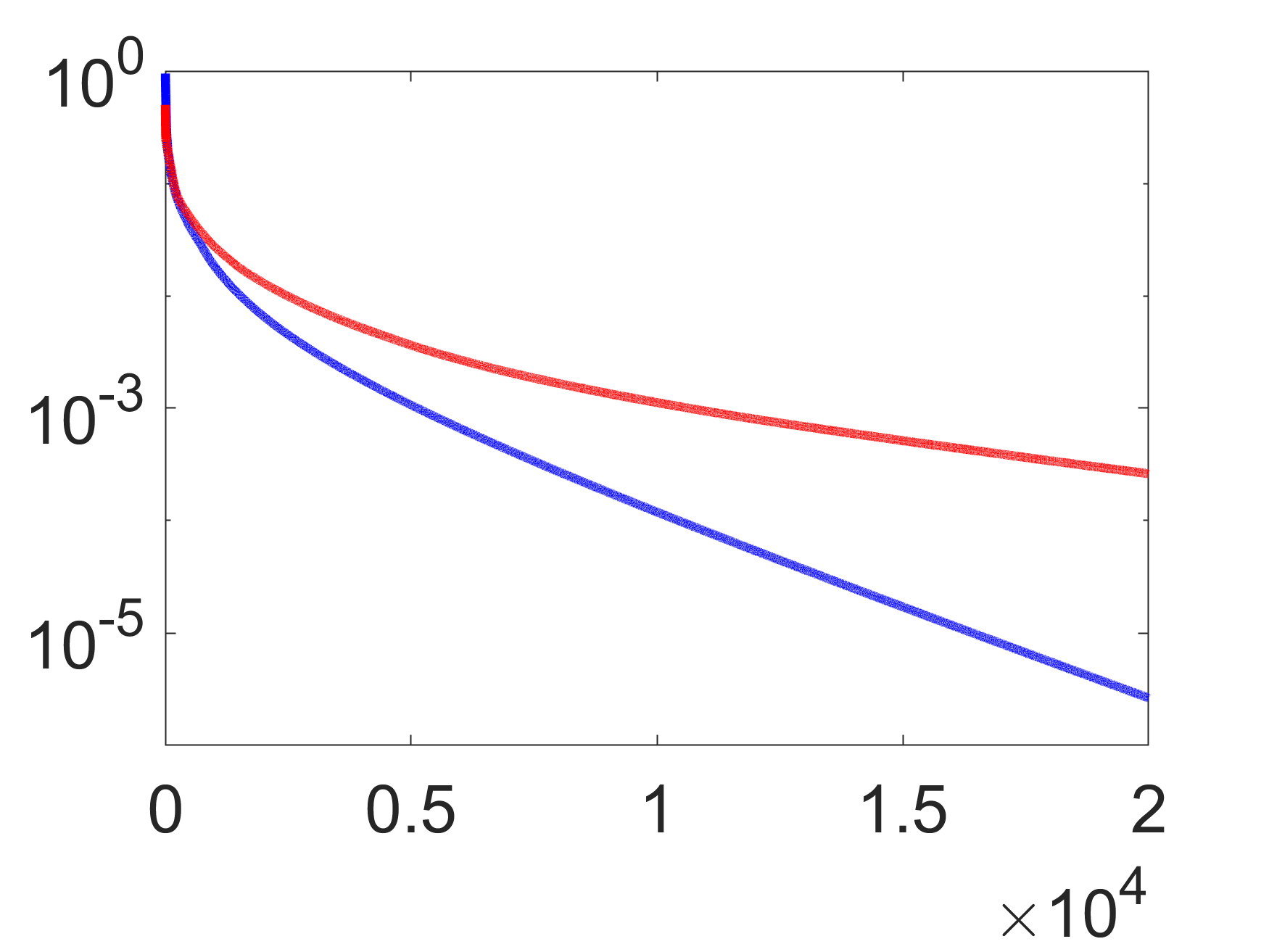
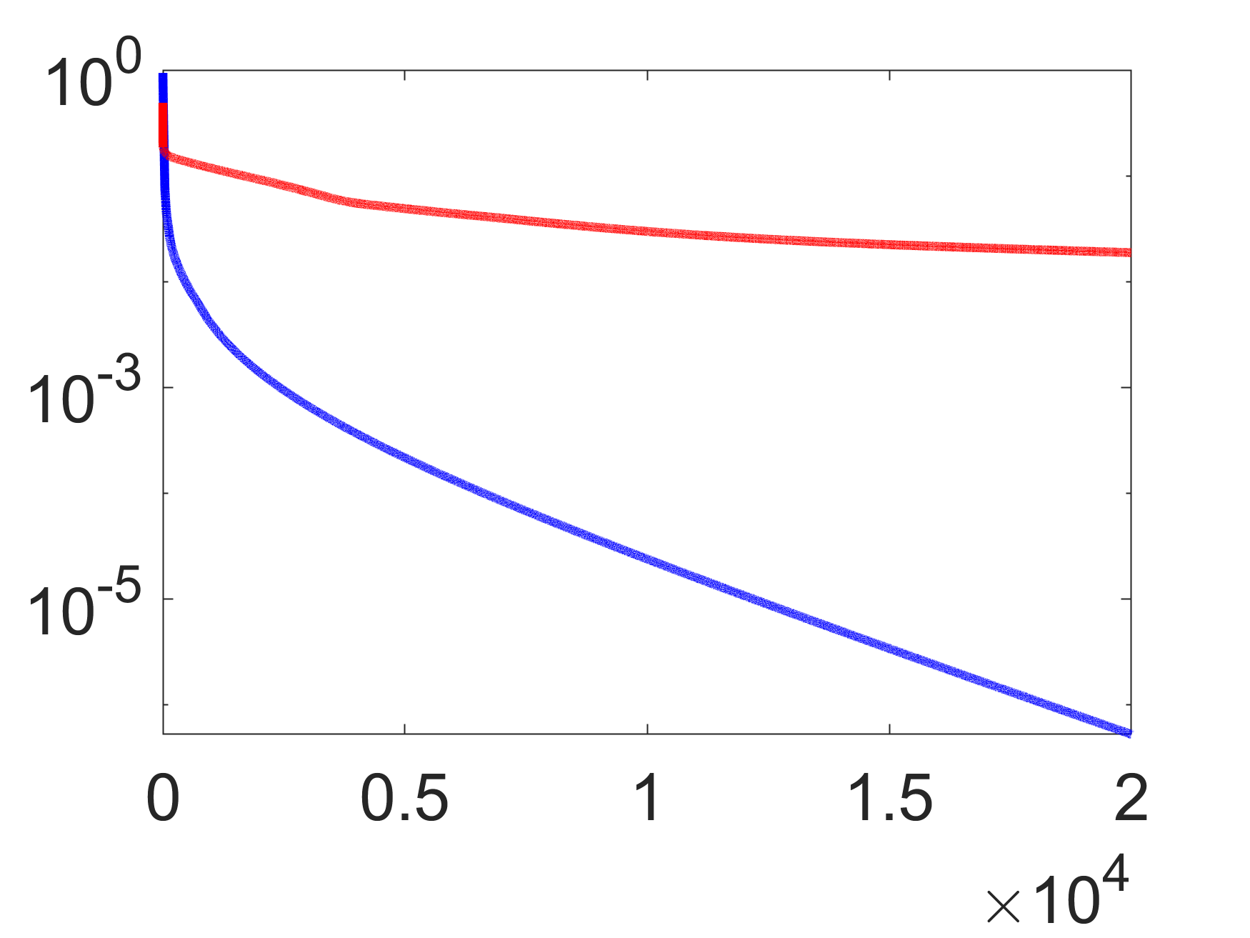
$\dfrac{f(K^{k})-f(K^{\star})}{f(K^{0})-f(K^{\star})}$	$k$		$k$

Figure 2: Convergence curves for gradient descent (blue) over the set $\mathcal{S}_{K}$, and gradient descent (red) over the set $\mathcal{S}_{Y}$ with (a) $s=10$ and (b) $s=20$ masses.

VIII-B Unknown model

To illustrate our results on the accuracy of the gradient estimation in Algorithm 1 and the efficiency of our random search method, we consider the LQR problem with $Q$ and $R$ equal to identity for $s=10$ masses (i.e., $n=20$ state variables). We also let the initial conditions $x_{i}$ in Algorithm 1 be standard normal and use $N=n=2s$ samples.

Figure 3 illustrates the dependence of the relative error $\|\widehat{\nabla}f(K)-\macc@depth\char 1\relax\frozen@everymath{\macc@group}\macc@set@skewchar\macc@nested@a 111{\nabla}f(K)\|_{F}/\|\widehat{\nabla}f(K)\|_{F}$ on the simulation time $\tau$ for $K=0$ and two values of the smoothing parameter $r=10^{-4}$ (blue) and $r=10^{-5}$ (red). We observe an exponential decrease in error for small values of $\tau$. In addition, the error does not pass a saturation level which is determined by $r$. We also see that, as $r$ decreases, this saturation level becomes smaller. These observations are in harmony with our theoretical developments; in particular, combining Propositions 4 and 5 through the use of the triangle inequality yields

$$\|\widehat{\nabla}f(K)\,-\,\macc@depth\char 1\relax\frozen@everymath{\macc@group}\macc@set@skewchar\macc@nested@a 111{\nabla}f(K)\|_{F}\;\leq\;\left(\dfrac{\sqrt{mn}}{r}\,\kappa_{1}(2a)\,\mathrm{e}^{-\kappa_{2}(2a)\tau}\,+\,\dfrac{r^{2}m^{2}n^{2}}{2}\,\ell(2a)\right)\max_{i}\|x_{i}\|^{2}.$$

This upper bound clearly captures the exponential dependence of the bias on the simulation time $\tau$ as well as the saturation level that depends quadratically on the smoothing parameter $r$.

In Fig. 3, we demonstrate the dependence of the total relative error $\|\nabla f(K)-\macc@depth\char 1\relax\frozen@everymath{\macc@group}\macc@set@skewchar\macc@nested@a 111{\nabla}f(K)\|_{F}/\|\nabla f(K)\|_{F}$ on the simulation time $\tau$ for two values of the smoothing parameter $r=10^{-4}$ (blue) and $r=10^{-5}$ (red), resulting from the use of $N=n$ samples. We observe that the distance between the approximate gradient and the true gradient is rather large. This is exactly why prior analysis of sample complexity and simulation time is subpar to our results. In contrast to the existing results which rely on the use of the estimation error shown in Fig. 3, our analysis shows that the simulated gradient $\macc@depth\char 1\relax\frozen@everymath{\macc@group}\macc@set@skewchar\macc@nested@a 111{\nabla}f(K)$ is close to the gradient estimate $\widehat{\nabla}f(K)$. While $\widehat{\nabla}f(K)$ is not close to the true gradient $\nabla f(K)$, it is highly correlated with it. This is sufficient for establishing convergence guarantees and it allows us to significantly improve upon existing results [12, 13] in terms of sample complexity and simulation time reducing both to $O(\log\,(1/\epsilon))$.

Finally, Fig. 3 demonstrates linear convergence of the random search method (RS) with stepsize $\alpha=10^{-4}$, $r=10^{-5}$, and $\tau=200$ in Algorithm 1, as established in Theorem 4. In this experiment, we implemented Algorithm 1 using the $\mathrm{ode45}$ and $\mathrm{trapz}$ subroutines in MATLAB to numerically integrate the state/input penalties with the corresponding weight matrices $Q$ and $R$. However, our theoretical results only account for an approximation error that arises from a finite simulation horizon. Clearly, employing empirical ODE solvers and numerical integration may introduce additional errors in our gradient approximation that require further scrutiny.

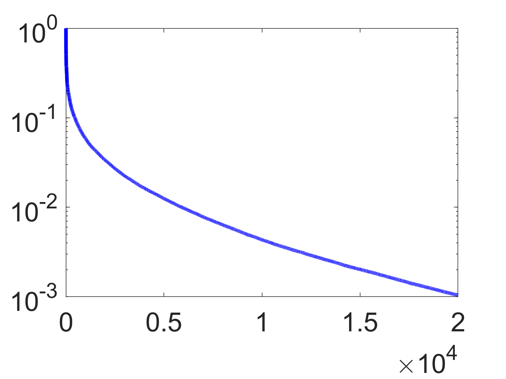
$\dfrac{\|\widehat{\nabla}f(K)-\macc@depth\char 1\relax\frozen@everymath{\macc@group}\macc@set@skewchar\macc@nested@a 111{\nabla}f(K)\|_{F}}{\|\widehat{\nabla}f(K)\|_{F}}$	$\tau$	$\dfrac{\|\nabla f(K)-\macc@depth\char 1\relax\frozen@everymath{\macc@group}\macc@set@skewchar\macc@nested@a 111{\nabla}f(K)\|_{F}}{\|\nabla f(K)\|_{F}}$	$\tau$	$\dfrac{f(K^{k})-f(K^{\star})}{f(K^{0})-f(K^{\star})}$	$k$

Figure 3: (a) Bias in gradient estimation and (b) total error in gradient estimation as functions of the simulation time $\tau$. The blue and red curves correspond to two values of the smoothing parameter $r=10^{-4}$ and $r=10^{-5}$, respectively. (c) Convergence curve of the random search method (RS).

IX Concluding remarks

We prove exponential/linear convergence of gradient flow/descent algorithms for solving the continuous-time LQR problem based on a nonconvex formulation that directly searches for the controller. A salient feature of our analysis is that we relate the gradient-flow dynamics associated with this nonconvex formulation to that of a convex reparameterization. This allows us to deduce convergence of the nonconvex approach from its convex counterpart. We also establish a bound on the sample complexity of the random search method for solving the continuous-time LQR problem that does not require the knowledge of system parameters. We have recently proved similar result for the discrete-time LQR problem [41].

Our ongoing research directions include: (i) providing theoretical guarantees for the convergence of gradient-based methods for sparsity-promoting and structured control synthesis; and (ii) extension to nonlinear systems via successive linearization techniques.

-A Lack of convexity of function $f$

The function $f$ is nonconvex in general because its effective domain, namely, the set of stabilizing feedback gains $\mathcal{S}_{K}$ can be nonconvex. In particular, for $A=0$ and $B=-I$, the closed-loop $A$-matrix is given by $A-BK=K$. Now, let

$$K_{1}\;=\;\left[\begin{array}[]{cc}-1&2-2\epsilon\\ 0&-1\end{array}\right],\qquad K_{2}\;=\;\left[\begin{array}[]{cc}-1&0\\ 2-2\epsilon&-1\end{array}\right],\qquad K_{3}\;=\;\dfrac{K_{1}+K_{2}}{2}=\left[\begin{array}[]{cc}-1&1-\epsilon\\ 1-\epsilon&-1\end{array}\right]$$ (43)

where $0\leq\epsilon\ll 1$. It is straightforward to show that for $\epsilon>0$, the entire line-segment $\overline{K_{1}K_{2}}$ lies in $\mathcal{S}_{K}$. However, if we let $\epsilon\rightarrow 0$, while the endpoints $K_{1}$ and $K_{2}$ converge to stabilizing gains, the middle point $K_{3}$ converges to the boundary of $\mathcal{S}_{K}$. Thus, $f(K_{1})$ and $f(K_{2})$ are bounded whereas $f(K_{3})\rightarrow\infty$. This implies the existence of a point on the line-segment $\overline{K_{1}K_{2}}$ for some $\epsilon\ll 1$ for which the function $f$ has negative curvature. For $\epsilon=0.1$, Fig. 4 illustrates the value of the LQR objective function $f(K(\gamma))$ associated with the above example and the problem parameters $Q=R=\Omega=I$, where $K(\gamma)\mathrel{\mathop{:}}=\gamma{K_{1}}+(1-\gamma){K_{2}}$ is the line-segment $\overline{K_{1}K_{2}}$. We observe the negative curvature of $f$ around the middle point $K_{3}$. Alternatively, we can verify the negative curvature using the second-order term $\left\langle J,\nabla^{2}f(K);J\right\rangle$ in the Taylor series expansion of $f(K+J)$ around $K$ given in Appendix -G. For the above example, letting $J=(K_{1}-K_{2})/\|K_{1}-K_{2}\|$ yields the negative value $\left\langle J,\nabla^{2}f(K_{3});J\right\rangle=-135.27$.

$f(K({\gamma}))$

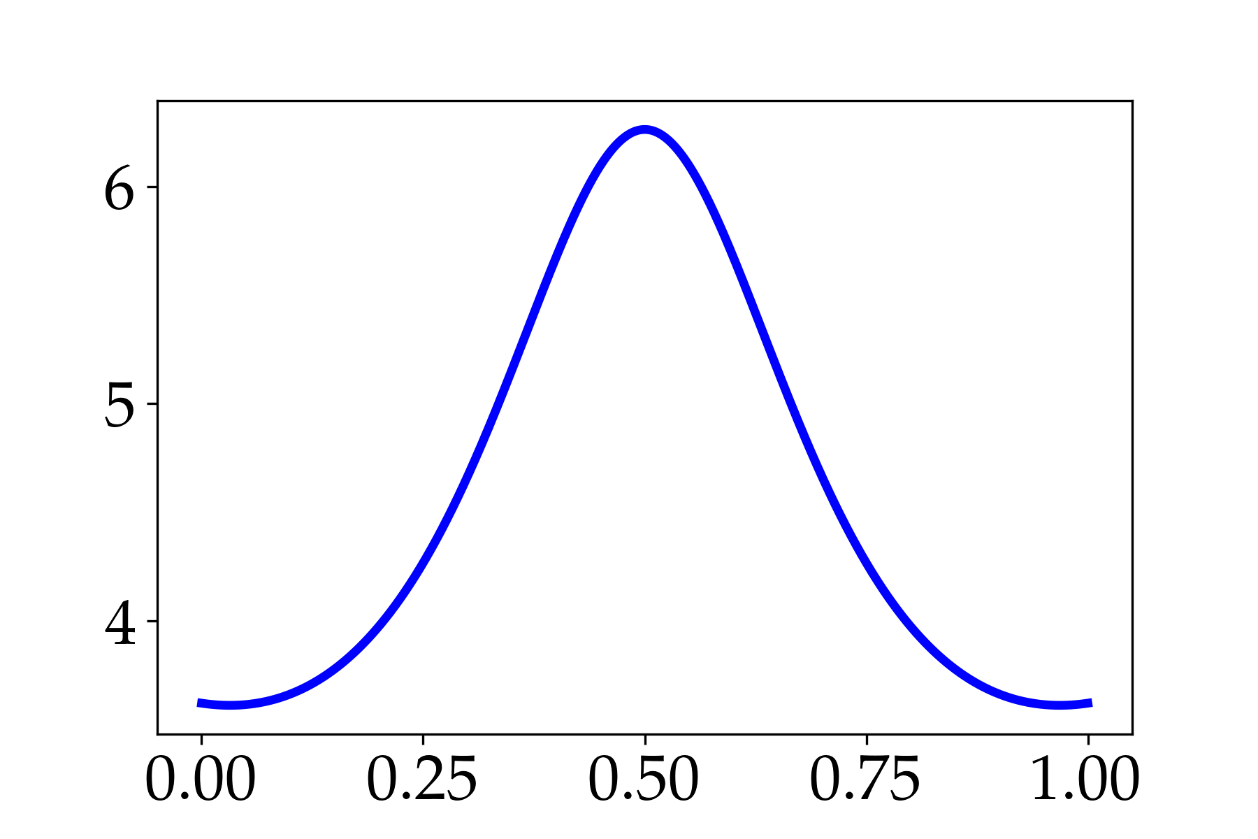
$\gamma$

Figure 4: The LQR objective function $f(K(\gamma))$, where $K(\gamma)\mathrel{\mathop{:}}=\gamma{K_{1}}+(1-\gamma){K_{2}}$ is the line-segment between $K_{1}$ and $K_{2}$ in (43) with $\epsilon=0.1$.

-B Invertibility of the linear map ${\cal A}$

The invertibility of the map ${\cal A}$ is equivalent to the matrices $A$ and $-A^{T}$ not having any common eigenvalues. If ${\cal A}$ is non-invertible, we can use $K^{0}\in\mathcal{S}_{K}$ to introduce the change of variables $\hat{K}\mathrel{\mathop{:}}=K-K^{0}$ and $\hat{Y}\mathrel{\mathop{:}}=\hat{K}X$ and obtain $f(K)=\hat{h}(X,\hat{Y})\mathrel{\mathop{:}}=\mathrm{trace}\,(Q^{0}X+X^{-1}\hat{Y}^{T}R\,\hat{Y}+2\hat{Y}^{T}RK^{0})$ for all $K\in\mathcal{S}_{K}$, where $Q^{0}\mathrel{\mathop{:}}=Q+(K^{0})^{T}R\,K^{0}$. Moreover, $X$ and $\hat{Y}$ satisfy the affine relation ${\cal A}_{0}(X)-{\cal B}(\hat{Y})+\Omega=0,$ where ${\cal A}_{0}(X)\mathrel{\mathop{:}}=(A-BK^{0})X+X(A-BK^{0})^{T}$. Since the matrix $A-BK^{0}$ is Hurwitz, the map ${\cal A}_{0}$ is invertible. This allows us to write $X$ as an affine function of $\hat{Y}$, $X(\hat{Y})={\cal A}_{0}^{-1}({\cal B}(\hat{Y})-\Omega).$ Since the function $\hat{h}(\hat{Y})\mathrel{\mathop{:}}=\hat{h}(X(\hat{Y}),\hat{Y})$ has a similar form to $h(Y)$ except for the linear term $2\,\mathrm{trace}\,(\hat{Y}^{T}R\,K^{0})$, the smoothness and strong convexity of $h(Y)$ established in Proposition 1 carry over to the function $\hat{h}(Y)$.

-C Proof of Proposition 1

The second-order term in the Taylor series expansion of $h(Y+\tilde{Y})$ around $Y$ is given by [30, Lemma 2]

$$\left\langle\tilde{Y},\nabla^{2}h(Y;\tilde{Y})\right\rangle\;=\;2\,\|R^{\frac{1}{2}}(\tilde{Y}\,-\,K\tilde{X})X^{-\frac{1}{2}}\|_{F}^{2}$$ (44)

where $\tilde{X}$ is the unique solution to ${\cal A}(\tilde{X})={\cal B}(\tilde{Y}).$ We show that this term is upper and lower bounded by $L\|\tilde{Y}\|_{F}^{2}$ and $\mu\|\tilde{Y}\|_{F}^{2}$, where $L$ and $\mu$ are given by (10a) and (10b), respectively. The proof for the upper bound is borrowed from [30, Lemma 1]; we include it for completeness. We repeatedly use the bounds on the variables presented in Lemma 23; see Appendix -K.

Smoothness

For any $Y\in\mathcal{S}_{Y}(a)$ and $\tilde{Y}$ with $\|\tilde{Y}\|_{F}=1$,

$$\left\langle\tilde{Y},\nabla^{2}h(Y;\tilde{Y})\right\rangle \;=\;2\|R^{\tfrac{1}{2}}(\tilde{Y}\,-\,K\tilde{X})X^{-\tfrac{1}{2}}\|_{F}^{2}\;\leq\;2\|R\|_{2}\|X^{-1}\|_{2}\|\tilde{Y}\,-\,K{\cal A}^{-1}{\cal B}(\tilde{Y})\|_{F}^{2}$$

$$\leq\;\dfrac{2\,\|R\|_{2}}{\lambda_{\min}(X)}\left(\|\tilde{Y}\|_{F}\,+\,\|K\|_{2}\|{\cal A}^{-1}{\cal B}\|_{2}\|\tilde{Y}\|_{F}\right)^{2}\;\leq\;\dfrac{2a\|R\|_{2}}{\nu}\left(1\,+\,\dfrac{a\|{\cal A}^{-1}{\cal B}\|_{2}}{\sqrt{\nu\lambda_{\min}(R)}}\right)^{2}=\mathrel{\mathop{:}}\;L.$$

Here, the first and second inequalities are obtained from the definition of the $2$-norm in conjunction with the triangle inequality, and the third inequality follows from (80b) and (80c). This completes the proof of smoothness.

Strong convexity

Using the positive definiteness of matrices $R$ and $X$, the second-order term (44) can be lower bounded by

$$\left\langle\tilde{Y},\nabla^{2}h(Y;\tilde{Y})\right\rangle\;\geq\;\dfrac{2\lambda_{\min}(R)\|H\|_{F}^{2}}{\|X\|_{2}}$$ (45)

where $H\mathrel{\mathop{:}}=\tilde{Y}-K\tilde{X}$. Next, we show that

$$\dfrac{\|H\|_{F}}{\|\tilde{X}\|_{F}}\;\geq\;\dfrac{\lambda_{\min}(\Omega)\lambda_{\min}(\Omega)}{a\,\|{\cal B}\|_{2}}.$$ (46)

We substitute $H+K\tilde{X}$ for $\tilde{Y}$ in ${\cal A}(\tilde{X})={\cal B}(\tilde{Y})$ to obtain

$$\Gamma\;=\;{\cal B}(H)$$ (47)

where $\Gamma\mathrel{\mathop{:}}={\cal A}_{K}(\tilde{X}).$ The closed-loop stability implies $\tilde{X}={\cal A}_{K}^{-1}(\Gamma)$ and from Eq. (47) we have

$$\|H\|_{F} \;\geq\;\dfrac{\|\Gamma\|_{F}}{\|{\cal B}\|_{2}}.$$ (48)

This allows us to use Lemma 25, presented in Appendix -L, to write $a\|\Gamma\|_{F}\geq\lambda_{\min}(\Omega)\lambda_{\min}(Q)\|\tilde{X}\|_{F}.$ This inequality in conjunction with (48) yield (46). Next, we derive an upper bound on $\|\tilde{Y}\|_{F}$,

$$\|\tilde{Y}\|_{F}\;=\;\|H\,+\,K\tilde{X}\|_{F}\;\leq\;\|H\|_{F}\,+\,\|K\|_{F}\|\tilde{X}\|_{F}\;\leq\;\|H\|_{F}\left(1\,+\,a^{2}\eta\right)$$ (49)

where $\eta$ is given by (10c) and the second inequality follows from (80d) and (46). Finally, inequalities (45) and (49) yield

$$\dfrac{\left\langle\tilde{Y},\nabla^{2}f(Y;\tilde{Y})\right\rangle}{\|\tilde{Y}\|_{F}^{2}}\;\geq\;\dfrac{2\lambda_{\min}(R)\|H\|_{F}^{2}}{\|X\|_{2}\|\tilde{Y}\|_{F}^{2}}\;\geq\;\dfrac{2\lambda_{\min}(R)}{\|X\|_{2}(1\,+\,a^{2}\eta)^{2}}\;\geq\;\dfrac{2\lambda_{\min}(R)\lambda_{\min}(Q)}{a(1\,+\,a^{2}\eta)^{2}}\;=\mathrel{\mathop{:}}\;\mu$$ (50)

where the last inequality follows from (80a).

-D Proofs for Section V

Proof of Lemma 1

The gradients are given by $\nabla f(K)=EX$ and $\nabla h(Y)=E+2B^{T}(P-W)$, where $E\mathrel{\mathop{:}}=2(RK-B^{T}P)$, $P$ is determined by (6a), and $W$ is the solution to (11b). Subtracting (11b) from (6b) yields $A^{T}(P-W)+(P-W)A=-\tfrac{1}{2}\left(K^{T}E+E^{T}K\right),$ which in turn leads to

$$\|P-W\|_{F}\;\leq\;\|{\cal A}^{-1}\|_{2}\|K\|_{F}\|E\|_{F}\;\leq\;\dfrac{a\|{\cal A}^{-1}\|_{2}\|E\|_{F}}{\sqrt{\nu\lambda_{\min}(R)}}$$

where the second inequality follows from (80d) in Appendix -K. Thus, by applying the triangle inequality to $\nabla h(Y)$, we obtain

$$\dfrac{\|\nabla h(Y)\|_{F}}{\|E\|_{F}}\;\leq\;1\,+\,\dfrac{2a\|{\cal A}^{-1}\|_{2}\|B\|_{2}}{\sqrt{\nu\lambda_{\min}(R)}}.$$

Moreover, using the lower bound (80c) on $\lambda_{\min}(X)$, we have $\|\nabla f(K)\|_{F}=\|EX\|_{F}\geq(\nu/a)\|E\|_{F}.$ Combining the last two inequalities completes the proof.

Proof of Lemma 2

For any pair of stabilizing feedback gains $K$ and $\hat{K}\mathrel{\mathop{:}}=K+\tilde{K}$, we have [32, Eq. (2.10)], $f(\hat{K})-f(K)=\mathrm{trace}\big{(}\tilde{K}^{T}\big{(}R(K+\hat{K})-2B^{T}\hat{P}\big{)}X\big{)},$ where $X=X(K)$ and $\hat{P}=P(\hat{K})$ are given by (4a) and (6a), respectively. Letting $\hat{K}=K^{\star}$ in this equation and using the optimality condition $B^{T}\hat{P}=R\hat{K}$ completes the proof.

Proof of Lemma 3

We show that the second-order term $\left\langle\tilde{K},\nabla^{2}f(K;\tilde{K})\right\rangle$ in the Taylor series expansion of $f(K+\tilde{K})$ around $K$ is upper bounded by $L_{f}\|\tilde{K}\|_{F}^{2}$ for all $K\in\mathcal{S}_{K}(a)$. From [42, Eq. (2.3)], it follows

$$\left\langle\tilde{K},\nabla^{2}f(K;\tilde{K})\right\rangle\;=\;2\,\mathrm{trace}\,(\tilde{K}^{T}R\,\tilde{K}X-2\tilde{K}^{T}B^{T}\tilde{P}X)$$

where $\tilde{P}=({\cal A}_{K}^{*})^{-1}(C)$ and $C\mathrel{\mathop{:}}=\tilde{K}^{T}(B^{T}P-RK)+(B^{T}P-RK)^{T}\tilde{K}.$ Here, $X=X(K)$ and $P=P(K)$ are given by (4a) and (6a) respectively. Thus, using basic properties of the matrix trace and the triangle inequality, we have

$$\dfrac{\left\langle\tilde{K},\nabla^{2}f(K;\tilde{K})\right\rangle}{\|\tilde{K}\|_{F}^{2}}\,\leq\,2\|X\|_{2}\left(\|R\|_{2}+\dfrac{2\|B\|_{2}\|\tilde{P}\|_{F}}{\|\tilde{K}\|_{F}}\right).$$ (51)

Now, we use Lemma 25 to upper bound the norm of $\tilde{P}$, $\|\tilde{P}\|_{F}\leq{a}\|C\|_{F}/(\lambda_{\min}(\Omega)\lambda_{\min}(Q)).$ Moreover, from the definition of $C$, the triangle inequality, and the submultiplicative property of the $2$-norm, we have $\|C\|_{F}\leq 2\|\tilde{K}\|_{F}(\|B\|_{2}\|P\|_{2}+\|R\|_{2}\|K\|_{2})$ Combining the last two inequalities gives

$$\dfrac{\|\tilde{P}\|_{F}}{\|\tilde{K}\|_{F}}\;\leq\;\dfrac{2a}{\lambda_{\min}(\Omega)\lambda_{\min}(Q)}\,(\|B\|_{2}\|P\|_{2}+\|R\|_{2}\|K\|_{2})$$

which in conjunction with (51) lead to

$$\dfrac{\left\langle\tilde{K},\nabla^{2}f(K;\tilde{K})\right\rangle}{\|\tilde{K}\|_{F}^{2}}\;\leq\;2\|X\|_{2}\left(\|R\|_{2}\,+\,\dfrac{4a}{\lambda_{\min}(\Omega)\lambda_{\min}(Q)}\,(\|B\|^{2}_{2}\|P\|_{2}+\|B\|_{2}\|R\|_{2}\|K\|_{2})\right).$$

Finally, we use the bounds provided in Appendix -K to obtain

$$\dfrac{\left\langle\tilde{K},\nabla^{2}f(K;\tilde{K})\right\rangle}{\|\tilde{K}\|_{F}^{2}}\;\leq\;\dfrac{2a\|R\|_{2}}{\lambda_{\min}(Q)}\;+\;\dfrac{8a^{3}}{\lambda_{\min}^{2}(Q)\lambda_{\min}(\Omega)}\left(\dfrac{\|B\|_{2}^{2}}{\lambda_{\min}(\Omega)}\,+\,\dfrac{\|B\|_{2}\|R\|_{2}}{\sqrt{\nu\lambda_{\min}(R)}}\right)$$

which completes the proof.

-E Proofs for Section VI-A1

We first present two technical lemmas.

Lemma 9

Let $Z\succ 0$ and let the Hurwitz matrix $F$ satisfy

$$\left[\begin{array}[]{cc}\delta^{2}I+F^{T}Z+ZF&Z\\ Z&-I\end{array}\right]\;\prec\;0.$$ (54)

Then $F+\delta\Delta$ is Hurwitz for all $\Delta$ with $\|\Delta\|_{2}\leq 1$.

Proof:

The matrix $F+\delta\Delta$ is Hurwitz if and only if the linear map from $w$ to $x$ with the state-space realization $\{\dot{x}=Fx+w+u,$ $z=\delta x\}$ in feedback with $u=\Delta z$ is input-output stable. From the small-gain theorem [10, Theorem 8.2], this system is stable for all $\Delta$ in the unit ball if and only if the induced gain of the map $u\mapsto z$ with the state-space realization $\{\dot{x}=Fx+u,$ $z=\delta x\}$ is smaller than one. The KYP Lemma [10, Lemma 7.4] implies that this norm condition is equivalent to (54). ∎

Lemma 10

Let the matrices $F$, $X\succ 0$, and $\Omega\succ 0$ satisfy

$$FX\,+\,XF^{T}\,+\,\Omega\;=\;0.$$ (55)

Then the matrix $F+\Delta$ is Hurwitz for all $\Delta$ that satisfy $\|\Delta\|_{2}<{\lambda_{\min}(\Omega)}/(2\|X\|_{2}).$

Proof:

From (55), we obtain that $F$ is Hurwitz and $F\hat{X}+\hat{X}F^{T}+I\preceq 0$ where $\hat{X}\mathrel{\mathop{:}}=X/\lambda_{\min}(\Omega)$. Multiplication of this inequality from both sides by $\hat{X}^{-1}$ and division by $2$ yields $ZF+F^{T}Z+2\,Z^{2}\preceq 0$ where $Z\mathrel{\mathop{:}}=(2\hat{X})^{-1}$. For any positive scalar $\delta<\lambda_{\min}(Z)={\lambda_{\min}(\Omega)}/(2\|X\|_{2})$ the last matricial inequality implies $\delta^{2}I+ZF+F^{T}Z+Z^{2}\prec 0.$ The result follows from Lemma 9 by observing that the last inequality is equivalent to (54) via the use of Schur complement. ∎

Proof of Proposition 3

For any feedback gain $\hat{K}$ such that $\|\hat{K}-K\|_{2}<\zeta$, the closed-loop matrix $A-B\hat{K}$ satisfies $\|A-B\hat{K}-(A-BK)\|_{2}\leq\|K-\hat{K}\|_{2}\|B\|_{2}<\zeta\|B\|_{2}.$ This bound on the distance between the closed-loop matrices $A-BK$ and $A-B\hat{K}$ allows us to apply Lemma 10 with $F\mathrel{\mathop{:}}=A-BK$ and $X\mathrel{\mathop{:}}=X(K)$ to complete the proof.

We next present a technical lemma.

Lemma 11

For any $K\in\mathcal{S}_{K}$ and $\hat{K}\in\mathbb{R}^{m\times n}$ such that $\|\hat{K}-K\|_{2}<\delta$, with

$$\delta\,\mathrel{\mathop{:}}=\,\dfrac{1}{4\,\|B\|_{F}}\,\min\left\{\dfrac{\lambda_{\min}(\Omega)}{\mathrm{trace}\,(X(K))},\,\dfrac{\lambda_{\min}(Q)}{\mathrm{trace}\,(P(K))}\right\}$$

the feedback gain matrix $\hat{K}\in\mathcal{S}_{K}$, and

$$\|X(\hat{K})\,-X(K)\|_{F} \;\leq\;\epsilon_{1}\|\hat{K}-K\|_{2}$$ (56a)

$$\|P(\hat{K})\,-P(K)\|_{F} \;\leq\;\epsilon_{2}\|\hat{K}-K\|_{2}$$ (56b)

$$\|\nabla f(\hat{K})\,-\nabla f(K)\|_{F} \;\leq\;\epsilon_{3}\|\hat{K}-K\|_{2}$$ (56c)

$$|f(\hat{K})\,-f(K)|~{}~{} \;\leq\;\epsilon_{4}\|\hat{K}-K\|_{2}$$ (56d)

where $X(K)$ and $P(K)$ are given by (4a) and (6a), respectively. Furthermore, the parameters $\epsilon_{i}$ which only depend on $K$ and problem data are given by $\epsilon_{1}\mathrel{\mathop{:}}={\|X(K)\|_{2}}/{\delta},$ $\epsilon_{2}\mathrel{\mathop{:}}={2\,\mathrm{trace}(P)}(2\,\|P\|_{2}\|B\|_{F}+(\delta+2\|K\|_{2})\|R\|_{F})/{\lambda_{\min}(Q)},$ $\epsilon_{4}\mathrel{\mathop{:}}=\epsilon_{2}\|\Omega\|_{F},$ $\epsilon_{3}\mathrel{\mathop{:}}=2(\epsilon_{1}\|K\|_{2}+2\|X(K)\|_{2})\|R\|_{F}+2\epsilon_{1}(\|P(K)\|_{2}+2\epsilon_{2}\|X(K)\|_{2})\|B\|_{F}.$

Proof:

Note that $\delta\leq\zeta$, where $\zeta$ is given in Proposition 3. Thus, we can use Proposition 3 to show that $\hat{K}\in\mathcal{S}_{K}$. We next prove (56a). For $K$ and $\hat{K}\in\mathcal{S}_{K}$, we can represent $X=X(K)$ and $\hat{X}=X(\hat{K})$ as the positive definite solutions to

$$(A\,-\,BK)X\;+\;X(A\,-\,BK)^{T}+\;\Omega \;=\;0$$ (57a)

$$(A\,-\,B\hat{K})\hat{X}\;+\;\hat{X}(A\,-\,B\hat{K})^{T}+\;\Omega \;=\;0.$$ (57b)

Subtracting (57a) from (57b) and rearranging terms yield

$$(A\,-\,BK)\tilde{X}\;+\;\tilde{X}(A\,-\,BK)^{T}\;=\;B\tilde{K}\hat{X}+\hat{X}(B\tilde{K})^{T}$$

where $\tilde{X}\mathrel{\mathop{:}}=\hat{X}-X$ and $\tilde{K}\mathrel{\mathop{:}}=\hat{K}-K$. Now, we use Lemma 24, presented in Appendix -L, with $F\mathrel{\mathop{:}}=A-BK$ to upper bound the norm of $\tilde{X}=\mathcal{F}(-B\tilde{K}\hat{X}-\hat{X}(B\tilde{K})^{T})$, where the linear map $\mathcal{F}$ is defined in (84), as follows

$${\|\tilde{X}\|_{F}} \;\leq\;\|\mathcal{F}\|_{2}\|B\tilde{K}\hat{X}+\hat{X}(B\tilde{K})^{T}\|_{F}\;\leq\;\dfrac{\mathrm{trace}(X)}{\lambda_{\min}(\Omega)}\|B\tilde{K}\hat{X}+\hat{X}(B\tilde{K})^{T}\|_{F}$$

$$\;\leq\;\dfrac{2\,\mathrm{trace}(X)\|B\|_{F}\|\tilde{K}\|_{2}}{\lambda_{\min}(\Omega)}\left(\|X\|_{2}+\|\tilde{X}\|_{2}\right)\;\leq\;\dfrac{2\,\mathrm{trace}(X)\|B\|_{F}\|\tilde{K}\|_{2}\|X\|_{2}}{\lambda_{\min}(\Omega)}\,+\,\dfrac{1}{2}\,\|\tilde{X}\|_{F}.$$ (58)

Here, the second inequality follows from Lemma 24, the third inequality follows from a combination of the sub-multiplicative property of the Frobenius norm and the triangle inequality, and the last inequality follows from $\|\tilde{K}\|\leq\delta$ and $\|\tilde{X}\|_{2}\leq\|\tilde{X}\|_{F}$. Rearranging the terms in (58) completes the proof of (56a).

We next prove (56b). Similar to the proof of (56a), subtracting the Lyapunov equation (6b) from that of $\hat{P}=P(\hat{K})$ yields $(A-BK)^{T}\tilde{P}+\tilde{P}(A-BK)=W$ where $\tilde{P}\mathrel{\mathop{:}}=\hat{P}-P$ and $W\mathrel{\mathop{:}}=(B\tilde{K})^{T}\hat{P}+\hat{P}B\tilde{K}-\tilde{K}^{T}R\,\tilde{K}-\tilde{K}^{T}R\,K-K^{T}R\,\tilde{K}.$ This allows us to use Lemma 24, presented in Appendix -L, with $F\mathrel{\mathop{:}}=(A-BK)^{T}$ to upper bound the norm of $\tilde{P}=\mathcal{F}(-W)$, where the linear map $\mathcal{F}$ is defined in (84), as follows

$${\|\tilde{P}\|_{F}}\;\leq\;\|\mathcal{F}\|_{2}\|W\|_{F}\;\leq\;\dfrac{\mathrm{trace}(\mathcal{F}(Q+K^{T}RK))}{\lambda_{\min}(Q+K^{T}RK)}\,\|W\|_{F}\;=\;\dfrac{\mathrm{trace}(P)}{\lambda_{\min}(Q+K^{T}RK)}\,\|W\|_{F}\;\leq\;\dfrac{\mathrm{trace}(P)}{\lambda_{\min}(Q)}\,\|W\|_{F}.$$

Here, the second inequality follows from Lemma 24. This inequality in conjunction with applying the triangle inequality to the definition of $W$ yield

$$\|\tilde{P}\|_{F}\;\leq\;\dfrac{\mathrm{trace}(P)}{\lambda_{\min}(Q)}\left(\|(B\tilde{K})^{T}\tilde{P}+\tilde{P}\,B\tilde{K}\|F\;+\;\|(B\tilde{K})^{T}P+P\,B\tilde{K}-\tilde{K}^{T}R\,\tilde{K}-\,\tilde{K}^{T}R\,K-\,K^{T}R\,\tilde{K}\|_{F}\right)\,\leq\\[0.0pt] \dfrac{\|\tilde{P}\|_{F}}{2}\;+\;\dfrac{\mathrm{trace}(P)}{\lambda_{\min}(Q)}\Big{(}2\|P\|_{2}\|B\|_{F}\,+\,(\delta+2\|K\|_{2})\|R\|_{F}\Big{)}\|\tilde{K}\|_{2}.$$

The second inequality is obtained by bounding the two terms on the left-hand side using basic properties of norm, where, for the first term, $\|\tilde{K}\|_{2}\leq\delta\leq{\lambda_{\min}(Q)}/(4\|B\|_{F}\,\mathrm{trace}\,(P(K)))$ and, for the second term, $\|\tilde{K}\|_{2}\leq\delta$. Rearranging the terms in above completes the proof of (56b).

We next prove (56c). It is straightforward to show that the gradient (5) satisfies

$$\tilde{\nabla}\;\mathrel{\mathop{:}}=\;\nabla f(\hat{K})-\nabla f(K)\;=\;2R(\tilde{K}X+K\tilde{X}+\tilde{K}\tilde{X})\,-\,2B^{T}(\tilde{P}X+P\tilde{X}+\tilde{P}\tilde{X})$$

where $P\mathrel{\mathop{:}}=P(K)$ and $\tilde{P}\mathrel{\mathop{:}}=\hat{P}-P$. The triangle inequality in conjunction with $\|\tilde{X}\|_{F}\leq\epsilon_{1}\|\tilde{K}\|_{2}$, $\|\tilde{P}\|_{F}\leq\epsilon_{2}\|\tilde{K}\|_{2}$, and $\|\tilde{K}\|_{2}<\delta$, yield ${\|\tilde{\nabla}\|_{F}}/{\|\tilde{K}\|_{2}}\leq 2\|R\|_{F}\,(\|X\|_{2}+\epsilon_{1}(\|K\|_{2}+\delta))+2\|B\|_{F}\,(\epsilon_{2}\|X\|_{2}+\epsilon_{1}(\|P\|_{2}+\epsilon_{2}\delta)).$ Rearranging terms completes the proof of (56c).

Finally, we prove (56d). Using the definitions of $f(K)$ in (3d) and $P(K)$ in (6a), it is easy to verify that $f(K)=\mathrm{trace}\,(P(K)\Omega).$ Application of the Cauchy-Schwartz inequality yields $|f(\hat{K})-f(K)|=|\mathrm{trace}\,(\tilde{P}\Omega)|\leq\|\tilde{P}\|_{F}\|\Omega\|_{F},$ which completes the proof. ∎

Proof of Lemma 4

For any $K\in\mathcal{S}_{K}(a)$, we can use the bounds provided in Appendix -K to show that $c_{1}/a\leq\delta$ and $\epsilon_{4}\leq c_{2}a^{2},$ where $\delta$ and $\epsilon_{4}$ are given in Lemma 11 and each $c_{i}$ is a positive constant that depends on the problem data. Now, Lemma 11 implies $f(K+r(a)U)-f(K)\leq\epsilon_{4}r(a)\|U\|_{2}\leq a$ where $r(a)\mathrel{\mathop{:}}=\min\{c_{1},1/c_{2}\}/(a\sqrt{mn}).$ This inequality together with $f(K)\leq a$ complete the proof.

-F Proof of Proposition 4

We first present two technical lemmas.

Lemma 12

Let the matrices $F$, $X\succ 0$, and $\Omega\succ 0$ satisfy $FX+XF^{T}+\Omega=0.$ Then, for any $t\geq 0$,

$$\|\mathrm{e}^{Ft}\|_{2}^{2}\;\leq\;(\|X\|_{2}/\lambda_{\min}(X))\,\mathrm{e}^{-(\lambda_{\min}(\Omega)/\|X\|_{2})\,t}.$$

Proof:

The function $V(x)\mathrel{\mathop{:}}=x^{T}Xx$ is a Lyapunov function for $\dot{x}=F^{T}x$ because $\dot{V}(x)={-x^{T}\Omega x}\leq-cV(x),$ where $c\mathrel{\mathop{:}}={\lambda_{\min}(\Omega)}/{\|X\|_{2}}$. For any initial condition $x_{0}$, this inequality together with the comparison lemma [35, Lemma 3.4] yield $V(x(t))\leq V(x_{0})\,\mathrm{e}^{-ct}.$ Noting that $x^{T}(t)=x_{0}^{T}\mathrm{e}^{Ft}$, we let $x_{0}$ be the normalized left singular vector associated with the maximum singular value of $\mathrm{e}^{Ft}$ to obtain

$$\|\mathrm{e}^{Ft}\|_{2}^{2}\;=\;\|x(t)\|^{2}\;\leq\;\dfrac{V(x(t))}{\lambda_{\min}(X)}\;\leq\;\dfrac{V(x_{0})}{\lambda_{\min}(X)}\,\mathrm{e}^{-ct}$$

which along with $V(x_{0})\leq\|X\|_{2}$ complete the proof. ∎

Lemma 13 establishes an exponentially decaying upper bound on the difference between $f_{x_{0}}(K)$ and $f_{x_{0},\tau}(K)$ over any sublevel set $\mathcal{S}_{K}(a)$ of the LQR objective function $f(K)$.

Lemma 13

For any $K\in\mathcal{S}_{K}(a)$ and $v\in\mathbb{R}^{n}$, $|f_{v}(K)-f_{v,\tau}(K)|\leq\|v\|^{2}\kappa_{1}(a)\mathrm{e}^{-\kappa_{2}(a)\tau},$ where the positive functions $\kappa_{1}(a)$ and $\kappa_{2}(a)$, given by (61), depend on problem data.

Proof:

Since $x(t)=\mathrm{e}^{(A-BK)t}v$ is the solution to (1b) with $u=-Kx$ and the initial condition $x(0)=v$, it is easy to verify that $f_{v,\tau}(K)=\mathrm{trace}\left((Q+K^{T}R\,K)\,X_{v,\tau}(K)\right)$ and $f_{v}(K)=\mathrm{trace}\left((Q\,+\,K^{T}R\,K)\,X_{v}(K)\right),$ where

$$X_{v,\tau}(K)\;\mathrel{\mathop{:}}=\;\int_{0}^{\tau}\mathrm{e}^{(A-BK)t}\,vv^{T}\mathrm{e}^{(A-BK)^{T}t}\,\mathrm{d}t$$

and $X_{v}\mathrel{\mathop{:}}=X_{v,\infty}.$ Using the triangle inequality, we have

$$\|X_{v}(K)-X_{v,\tau}(K)\|_{F}\,\leq\,\|v\|^{2}\int_{\tau}^{\infty}\|\mathrm{e}^{(A-BK)t}\|_{2}^{2}\;\mathrm{d}t.$$ (59)

Equation (4b) allows us to use Lemma 12 with $F\mathrel{\mathop{:}}=A-BK$, $X\mathrel{\mathop{:}}=X(K)$ to upper bound $\|\mathrm{e}^{(A-BK)t}\|_{2}$, ${\lambda_{\min}(X)}\|\mathrm{e}^{(A-BK)t}\|_{2}^{2}\leq{\|X\|_{2}}\,\mathrm{e}^{-(\lambda_{\min}(\Omega)/\|X\|_{2})\,t}.$ Integrating this inequality over $[\tau,\infty]$ in conjunction with (59) yield

$$\|X_{v}(K)-X_{v,\tau(K)}\|_{F} \;\leq\;\|v\|^{2}\kappa^{\prime}_{1}\,\mathrm{e}^{-\kappa^{\prime}_{2}\tau}$$ (60)

where $\kappa^{\prime}_{1}\mathrel{\mathop{:}}={\|X(K)\|_{2}^{2}}/(\lambda_{\min}(\Omega)\lambda_{\min}(X(K)))$ and $\kappa^{\prime}_{2}\mathrel{\mathop{:}}={\lambda_{\min}(\Omega)}/{\|X(K)\|_{2}}.$ Furthermore,

$$|f_{v}(K)-f_{v,\tau}(K)|\;=\;\left|\mathrm{trace}\left((Q+K^{T}R\,K)\,(X_{v}-X_{v,\tau})\right)\right|\;\leq\;\\[0.0pt] (\|Q\|_{F}+\|R\|_{2}\|K\|_{F}^{2})\|X_{v}-X_{v,\tau}\|_{F}\;\leq\;\|v\|^{2}(\|Q\|_{F}+\|R\|_{2}\|K\|_{F}^{2})\,\kappa^{\prime}_{1}\mathrm{e}^{-\kappa^{\prime}_{2}\tau}$$

where we use the Cauchy-Schwartz and triangle inequalities for the first inequality and (60) for the second inequality. Combining this result with the bounds on the variables provided in Lemma 23 completes the proof with

$$\kappa_{1}(a) \;\mathrel{\mathop{:}}=\;\left(\|Q\|_{F}+\dfrac{a^{2}\|R\|_{2}}{\nu\lambda_{\min}(R)}\right)\dfrac{a^{3}}{\nu\lambda_{\min}(\Omega)\lambda_{\min}^{2}(Q)}$$ (61a)

$$\kappa_{2}(a) \;\mathrel{\mathop{:}}=\;{\lambda_{\min}(\Omega)\lambda_{\min}(Q)}/{a}$$ (61b)

where the constant $\nu$ is given by (10d). ∎

Proof of Proposition 4

Since $K\in\mathcal{S}_{K}(a)$ and $r\leq r(a)$, Lemma 4 implies that $K\pm rU_{i}\in\mathcal{S}_{K}(2a)$. Thus, $f_{x_{i}}(K\pm rU_{i})$ is well defined for $i=1,\ldots,N$, and

$$\widetilde{\nabla}f(K)-\macc@depth\char 1\relax\frozen@everymath{\macc@group}\macc@set@skewchar\macc@nested@a 111{\nabla}f(K)\,=\,\dfrac{1}{2rN}\Big{(}\sum_{i}\big{(}f_{x_{i}}(K+rU_{i})-f_{x_{i},\tau}(K+rU_{i})\big{)}U_{i}-\sum_{i}\big{(}f_{x_{i}}(K-rU_{i})-f_{x_{i},\tau}(K-rU_{i})\big{)}U_{i}\Big{)}.$$

Furthermore, since $K\pm rU_{i}\in\mathcal{S}_{K}(2a)$, we can use triangle inequality and apply Lemma 13, $2N$ times, to bound each term individually and obtain

$$\|\widetilde{\nabla}f(K)-\macc@depth\char 1\relax\frozen@everymath{\macc@group}\macc@set@skewchar\macc@nested@a 111{\nabla}f(K)\|_{F}\;\leq\;(\sqrt{mn}/r)\max_{i}\|x_{i}\|^{2}\kappa_{1}(2a)\mathrm{e}^{-\kappa_{2}(2a)\tau}$$

where we used $\|U_{i}\|_{F}=\sqrt{mn}$. This completes the proof.

-G Proof of Proposition 5

We first establish bounds on the smoothness parameter of $\nabla f(K)$. For $J\in\mathbb{R}^{m\times n}$, $v\in\mathbb{R}^{n}$, and $f_{v}(K)$ given by (23a), let $j_{v}(K)\mathrel{\mathop{:}}=\left\langle J,\nabla^{2}f_{v}(K;J)\right\rangle,$ denote the second-order term in the Taylor series expansion of $f_{v}(K+J)$ around $K$. Following similar arguments as in [42, Eq. (2.3)] leads to $j_{v}(K)=2\,\mathrm{trace}\,(J^{T}(RJ-2B^{T}D)X_{v}),$ where $X_{v}$ and $D$ are the solutions to

$${\cal A}_{K}(X_{v}) \;=\;-vv^{T}$$ (62a)

$${\cal A}_{K}^{*}(D) \;=\;J^{T}(B^{T}P-R\,K)+(B^{T}P-R\,K)^{T}J$$ (62b)

and $P$ is given by (6a). The following lemma provides an analytical expression for the gradient $\nabla j_{v}(K)$.

Lemma 14

For any $v\in\mathbb{R}^{n}$ and $K\in\mathcal{S}_{K}$, $\nabla j_{v}(K)=4\big{(}B^{T}W_{1}X_{v}+(RJ-B^{T}D)W_{2}+(RK-B^{T}P)W_{3}\big{)},$ where $W_{i}$ are the solutions to the linear equations

$${\cal A}_{K}^{*}(W_{1}) \;=\;J^{T}R\,J-J^{T}B^{T}D-DBJ$$ (63a)

$${\cal A}_{K}(W_{2}) \;=\;BJX_{v}+X_{v}J^{T}B^{T}$$ (63b)

$${\cal A}_{K}(W_{3}) \;=\;BJ\,W_{2}+W_{2}J^{T}B^{T}.$$ (63c)

Proof:

We expand $j_{v}(K+\epsilon\tilde{K})$ around $K$ and to obtain $j_{v}(K+\epsilon\tilde{K})-j_{v}(K)=2\,\epsilon\,\mathrm{trace}\,(J^{T}(R\,J-2B^{T}D)\tilde{X}_{v})-4\,\epsilon\,\mathrm{trace}\,(J^{T}B^{T}\tilde{D}X_{v})+o(\epsilon).$ Here, $o(\epsilon)$ denotes higher-order terms in $\epsilon$, whereas $\tilde{X}_{v}$, $\tilde{D}$, and $\tilde{P}$ are obtained by perturbing Eqs. (62a), (62b), and (6b), respectively,

$$\!\!{\cal A}_{K}(\tilde{X}_{v}) \;=\;B\tilde{K}X_{v}+X_{v}\tilde{K}^{T}B^{T}$$ (64a)

$$\!\!{\cal A}_{K}^{*}(\tilde{D}) \;=\;\tilde{K}^{T}B^{T}D+DB\tilde{K}\;+\;{\cal A}_{K}^{*}(\tilde{D})\;=\;J^{T}(B^{T}\tilde{P}-R\tilde{K})+(B^{T}\tilde{P}-R\tilde{K})^{T}J$$ (64b)

$$\!\!{\cal A}_{K}^{*}(\tilde{P}) \;=\;\tilde{K}^{T}B^{T}P+PB\tilde{K}-K^{T}R\tilde{K}-\tilde{K}^{T}RK.$$ (64c)

Applying the adjoint identity on Eqs. (64a) and (64b) yields $j_{v}(K+\epsilon\tilde{K})-j_{v}(K)\approx 2\epsilon\,\mathrm{trace}\,((B\tilde{K}X_{v}+X_{v}\tilde{K}^{T}B^{T})W_{1})-2\epsilon\,\mathrm{trace}\,((\tilde{K}^{T}B^{T}D+DB\tilde{K}+J^{T}(B^{T}\tilde{P}-R\tilde{K})+(B^{T}\tilde{P}-R\tilde{K})^{T}J)W_{2})=4\epsilon\,\mathrm{trace}\,(\tilde{K}^{T}B^{T}W_{1}X_{v})-4\epsilon\,\mathrm{trace}\,(\tilde{K}^{T}(B^{T}D-RJ)W_{2})-4\epsilon\,\mathrm{trace}\,(W_{2}J^{T}B^{T}\tilde{P}),$ where we have neglected $o(\epsilon)$ terms, and $W_{1}$ and $W_{2}$ are given by (63a) and (63b), respectively. Moreover, the adjoint identity applied to (64c) allows us to simplify the last term as, $2\,\mathrm{trace}\,(W_{2}J^{T}B^{T}\tilde{P})=\mathrm{trace}\,((\tilde{K}^{T}B^{T}P+PB\tilde{K}-K^{T}R\tilde{K}-\tilde{K}^{T}RK)W_{3}),$ where $W_{3}$ is given by (63c). Finally, this yields $j(K+\epsilon\tilde{K})-j(K)\approx 4\epsilon\,\mathrm{trace}\,(\tilde{K}^{T}((RK-B^{T}P)W_{3}+B^{T}W_{1}X_{v}+(RJ-B^{T}D)W_{2})).$ ∎

We next establish a bound on $\|\nabla j_{v}(K)\|_{F}$.

Lemma 15

Let $K,K^{\prime}\in\mathbb{R}^{m\times n}$ be such that the line segment $K+t(K^{\prime}-K)$ with $t\in[0,1]$ belongs to $\mathcal{S}_{K}(a)$ and let $J\in\mathbb{R}^{m\times n}$ and $v\in\mathbb{R}^{n}$ be fixed. Then, the function $j_{v}(K)$ satisfies $|j_{v}(K_{1})-j_{v}(K_{2})|\leq\ell(a)\|J\|_{F}^{2}\|v\|^{2}\|K_{1}-K_{2}\|_{F},$ where $l(a)$ is a positive function given by

$$\ell(a)\,\mathrel{\mathop{:}}=\,ca^{2}\,+\,c^{\prime}a^{4}$$ (65)

and $c$, $c^{\prime}$ are positive scalars that depend only on problem data.

Proof:

We show that the gradient $\nabla j_{v}(K)$ given by Lemma 14 is upper bounded by $\|\nabla j_{v}(K)\|_{F}\leq\ell(a)\|J\|_{F}^{2}\|v\|^{2}$. Applying Lemma 25 on (62), the bounds in Lemma 23, and the triangle inequality, we have $\|X_{v}\|_{F}\leq c_{1}a\|v\|^{2}$ and $\|D\|_{F}\leq c_{2}a^{2}\|J\|_{F},$ where $c_{1}$ and $c_{2}$ are positive constants that depend on problem data. We can use the same technique to bound the norms of $W_{i}$ in Eq. (63), $\|W_{1}\|_{F}\leq(c_{3}a+c_{4}a^{3})\|J\|^{2}_{F},$ $\|W_{2}\|_{F}\leq c_{5}a^{2}\|v\|^{2}\|J\|_{F},$ $\|W_{3}\|_{F}\leq c_{6}a^{3}\|v\|^{2}\|J\|^{2}_{F},$ where $c_{3},\ldots,c_{6}$ are positive constants that depend on problem data. Combining these bounds with the Cauchy-Schwartz and triangle inequalities applied to $\nabla f_{v}(K)$ completes the proof. ∎

Proof of Proposition 5

Since $r\leq r(a)$, Lemma 4 implies that $K\pm sU\in\mathcal{S}_{K}(2a)$ for all $s\leq r$. Also, the mean-value theorem implies that, for any $U\in\mathbb{R}^{m\times n}$ and $v\in\mathbb{R}^{n}$,

$$f_{v}(K\pm rU)\;=\;f_{v}(K)\;\pm\;r\left\langle\nabla f_{v}(K),U\right\rangle\;+\;\dfrac{r^{2}}{2}\left\langle U,\nabla^{2}f_{v}(K\pm\,s_{\pm}\,U;U)\right\rangle$$

where $s_{\pm}\in[0,r]$ are constants that depend on $K$ and $U$. Now, if $\|U\|_{F}=\sqrt{mn}$, the above identity yields

$$\dfrac{1}{2r}{\left(f_{v}(K+rU)-f_{v}(K-rU)\right)}-\left\langle\nabla f_{v}(K),U\right\rangle\, \;=\;\dfrac{r}{4}\,(\left\langle U,\nabla^{2}f_{v}(K+s_{+}U;U)\right\rangle-\left\langle U,\nabla^{2}f_{v}(K-s_{-}U;U)\right\rangle)$$

$$\;\leq\;\dfrac{r}{4}\,(s_{+}+s_{-})\|U\|_{F}^{3}\,\ell(2a)\,\|v\|^{2}\,\leq\,\dfrac{r^{2}}{2}mn\sqrt{mn}\,\ell(2a)\,\|v\|^{2}$$

where the first inequality follows from Lemma 15. Combining this inequality with the triangle inquality applied to the definition of $\widehat{\nabla}f(K)-\widetilde{\nabla}f(K)$ completes the proof.

-H Proof of Proposition 6

From inequality (27a), it follows that $G$ is a descent direction of the function $f(K)$. Thus, we can use the descent lemma [37, Eq. (9.17)] to show that $K^{+}\mathrel{\mathop{:}}=K-\alpha G$ satisfies

$$\!f(K^{+})\,-\,f(K)\,\leq\,(L_{f}\alpha^{2}/2)\,\|G\|_{F}^{2}\,-\,\alpha\left\langle\nabla f(K),G\right\rangle$$ (66)

for any $\alpha$ for which the line segment between $K^{+}$ and $K$ lies in $\mathcal{S}_{K}(a)$. Using (27), for any $\alpha\in[0,2\mu_{1}/(\mu_{2}L_{f})]$, we have

$$(L_{f}\alpha^{2}/2)\,\|G\|_{F}^{2}\,-\,\alpha\left\langle\nabla f(K),G\right\rangle\;\leq\;(\alpha\,(L_{f}\mu_{2}\alpha-2\mu_{1})/2)\,\|\nabla f(K)\|_{F}^{2}\;\leq\;0$$ (67)

and the right-hand side of inequality (66) is nonpositive for $\alpha\in[0,2\mu_{1}/(\mu_{2}L_{f})]$. Thus, we can use the continuity of the function $f(K)$ along with inequalities (66) and (67) to conclude that $K^{+}\in\mathcal{S}_{K}(a)$ for all $\alpha\in[0,2\mu_{1}/(\mu_{2}L_{f})]$, and $f(K^{+})-f(K)\leq(\alpha\,(L_{f}\mu_{2}\alpha-2\mu_{1})/2)\,\|\nabla f(K)\|_{F}^{2}.$ Combining this inequality with the PL condition (17), it follows that, for any $\alpha\in[0,c_{1}/(c_{2}L_{f})]$,

$$f(K^{+})-f(K)\;\leq\;-(\mu_{1}\alpha/2)\,\|\nabla f(K)\|_{F}^{2}\leq-\mu_{f}\mu_{1}\alpha\,(f(K)-f(K^{\star})).$$

Subtracting $f(K^{\star})$ and rearranging terms complete the proof.

-I Proofs of Section VI-B1

We first present two technical results. Lemma 16 extends [43, Theorem 3.2] on the norm of Gaussian matrices presented in Appendix -J to random matrices with uniform distribution on the sphere $\sqrt{mn}\,S^{mn-1}$.

Lemma 16

Let $E\in\mathbb{R}^{m\times n}$ be a fixed matrix and let $U\in\mathbb{R}^{m\times n}$ be a random matrix with $\mathrm{vec}(U)$ uniformly distributed on the sphere $\sqrt{mn}\,S^{mn-1}$. Then, for any $s\geq 1$ and $t\geq 1$, we have $\mathbb{P}(\mathsf{B})\leq 2\mathrm{e}^{-s^{2}q-t^{2}n}+\mathrm{e}^{-mn/8}$, where $\mathsf{B}\mathrel{\mathop{:}}=\left\{\|E^{T}U\|_{2}>c^{\prime}\left(s\|E\|_{F}+t\sqrt{n}\|E\|_{2}\right)\right\},$ and $q\mathrel{\mathop{:}}=\|E\|_{F}^{2}/{\|E\|_{2}^{2}}$ is the stable rank of ${E}$.

Proof:

For a matrix $G$ with i.i.d. standard normal entries, we have $\|E^{T}U\|_{2}\sim\sqrt{mn}\|E^{T}G\|_{2}/{\|G\|_{F}}.$ Let the constant $\kappa$ be the $\psi_{2}$-norm of the standard normal random variable and let us define two auxiliary events, $\mathsf{C}_{1}\mathrel{\mathop{:}}=\{\sqrt{mn}>2\|G\|_{F}\}$ and $\mathsf{C}_{0}\mathrel{\mathop{:}}=\{\sqrt{mn}\,\|E^{T}G\|_{2}>2c\kappa^{2}\|G\|_{F}\left(s\|E\|_{F}+t\sqrt{n}\|E\|_{2}\right)\}.$ For $c^{\prime}\mathrel{\mathop{:}}=2c\kappa^{2}$, we have $\mathbb{P}(\mathsf{B})=\mathbb{P}(\mathsf{C}_{0})\leq\mathbb{P}(\mathsf{C}_{1}\cup\mathsf{A})\leq\mathbb{P}(\mathsf{C}_{1})+\mathbb{P}(\mathsf{A}),$ where the event $\mathsf{A}$ is given by Lemma 21. Here, the first inequality follows from $\mathsf{C}_{0}\subset\mathsf{C}_{1}\cup\mathsf{A}$ and the second follows from the union bound. Now, since $\|\cdot\|_{F}$ is Lipschitz continuous with parameter $1$, from the concentration of Lipschitz functions of standard normal Gaussian vectors [40, Theorem 5.2.2], it follows that $\mathbb{P}(C_{1})\leq\mathrm{e}^{-mn/8}$. This in conjunction with Lemma 21 complete the proof. ∎

Lemma 17

In the setting of Lemma 16, we have $\mathbb{P}\left\{\|{E}^{T}{U}\|_{F}>2\sqrt{n}\,\|{E}\|_{F}\right\}\leq\mathrm{e}^{-n/2}.$

Proof:

We begin by observing that $\|{E}^{T}{U}\|_{F}=\|\mathrm{vec}({E}^{T}{U})\|_{F}=\|\left({I}\otimes{E}^{T}\right)\mathrm{vec}(U)\|_{F},$ where $\otimes$ denotes the Kronecker product. Thus, it is easy to verify that $\|{E}^{T}{U}\|_{F}$ is a Lipschitz continuous function of ${U}$ with parameter $\|{I}\otimes{E}^{T}\|_{2}=\|{E}\|_{2}$. Now, from the concentration of Lipschitz functions of uniform random variables on the sphere $\sqrt{mn}\,S^{mn-1}$ [40, Theorem 5.1.4], for all $t>0$, we have $\mathbb{P}\,\big{\{}\|{E}^{T}{U}\|_{F}>\sqrt{\operatorname{\mathbb{E}}\left[\|{E}^{T}{U}\|_{F}^{2}\right]}+t\big{\}}\leq\mathrm{e}^{-{t^{2}}/(2\|E\|_{2}^{2})}.$ Now, since $\operatorname{\mathbb{E}}\,[\|E^{T}U\|^{2}_{F}]=\operatorname{\mathbb{E}}\,[\|({I}\otimes{E}^{T})\,\mathrm{vec}(U)\|_{F}^{2}]=\operatorname{\mathbb{E}}\,[\mathrm{trace}\,((I\otimes E^{T})\mathrm{vec}(U)\mathrm{vec}(U)^{T}(I\otimes E))]=\mathrm{trace}\,((I\otimes E^{T})(I\otimes E))=n\|E\|_{F}^{2},$ we can rewrite the last inequality for $t=\sqrt{n}\|E\|_{F}$ to obtain

$$\mathbb{P}\,\{\|E^{T}U\|_{F}>2\sqrt{n}\,\|E\|_{F}\}\,\leq\,\mathrm{e}^{-n\|E\|_{F}^{2}/(2\|E\|_{2}^{2})}\,\leq\,\mathrm{e}^{-{n}/{2}}$$

where the last inequality follows from $\|E\|_{F}\geq\|E\|_{2}.$ ∎

Proof of Lemma 5

We define the auxiliary events

$$\mathsf{D}_{i}\;\mathrel{\mathop{:}}=\;\{\|{\cal M}^{*}(E^{T}U_{i})\|_{2}\leq c\sqrt{n}\,\|M^{*}\|_{S}\|E\|_{F}\}\cap\{\|{\cal M}^{*}(E^{T}U_{i})\|_{F}\;\leq\;2\sqrt{n}\|M^{*}\|_{2}\|E\|_{F}\}$$

for $i=1,\ldots,N$. Since $\|{\cal M}^{*}(E^{T}U_{i})\|_{2}\leq\|{\cal M}^{*}\|_{S}\|E^{T}U_{i}\|_{2}$ and $\|{\cal M}^{*}(E^{T}U_{i})\|_{F}\leq\|{\cal M}^{*}\|_{2}\|E^{T}U_{i}\|_{F}$, we have $\mathbb{P}(\mathsf{D}_{i})\geq\{\|E^{T}U_{i}\|_{2}\leq c\sqrt{n}\|E\|_{F}\}\cap\{\|E^{T}U_{i}\|_{F}\leq 2\sqrt{n}\|E\|_{F}\}.$ Applying Lemmas 16 and 17 to the right-hand side of the above events together with the union bound yield $\mathbb{P}(\mathsf{D}_{i}^{c})\leq 2\mathrm{e}^{-n}+\mathrm{e}^{-{mn}/{8}}+\mathrm{e}^{-{n}/{2}}\leq 4\mathrm{e}^{-{n}/{8}},$ where $\mathsf{D}_{i}^{c}$ is the complement of $\mathsf{D}_{i}$. This in turn implies

$$\mathbb{P}(\mathsf{D}^{c})\;=\;\mathbb{P}(\bigcup_{i\,=\,1}^{N}\mathsf{D}_{i}^{c})\;\leq\;\sum_{i\,=\,1}^{N}\mathbb{P}(\mathsf{D}_{i}^{c})\;\leq\;4N\mathrm{e}^{-\tfrac{n}{8}}$$ (68)

where $\displaystyle\mathsf{D}\mathrel{\mathop{:}}=\cap_{i}\,\mathsf{D}_{i}$. We can now use the conditioning identity to bound the failure probability,

$$\mathbb{P}\{|a|>b\} \;=\;\mathbb{P}\left\{|a|>b\,\big{|}\,\mathsf{D}\right\}\mathbb{P}(\mathsf{D})+\mathbb{P}\left\{|a|>b\,\big{|}\,\mathsf{D}^{c}\right\}\mathbb{P}(\mathsf{D}^{c})$$

$$\;\leq\;\mathbb{P}\left\{|a|>b\,\big{|}\,\mathsf{D}\right\}\mathbb{P}(\mathsf{D})+\mathbb{P}(\mathsf{D}^{c})$$

$$\;=\;\mathbb{P}\left\{|a\,\mathds{1}_{\mathsf{D}}|\,>b\right\}\,+\,\mathbb{P}(\mathsf{D}^{c})$$

$$\;\leq\;\mathbb{P}\left\{|a\,\mathds{1}_{\mathsf{D}}|>b\right\}\,+\,4N\mathrm{e}^{-{n}/{8}}$$ (69)

where $a\mathrel{\mathop{:}}=(1/N)\sum_{i}\left\langle E\left(X_{i}-X\right),U_{i}\right\rangle\left\langle EX,U_{i}\right\rangle,$ $b\mathrel{\mathop{:}}=\delta\|EX\|_{F}\|E\|_{F}$, and $\mathds{1}_{\mathsf{D}}$ is the indicator function of $\mathsf{D}$. It is now easy to verify that $\mathbb{P}\{|a\,\mathds{1}_{\mathsf{D}}|>b\}\leq\mathbb{P}\left\{\left|Y\right|>b\right\},$ where $Y\mathrel{\mathop{:}}=(1/N)\sum_{i}Y_{i},$ $Y_{i}\mathrel{\mathop{:}}=\left\langle E(X_{i}-X),U_{i}\right\rangle\left\langle EX,U_{i}\right\rangle\mathds{1}_{\mathsf{D}_{i}}.$ The rest of the proof uses the $\psi_{{1}/{2}}$-norm of $Y$ to establish an upper bound on $\mathbb{P}\left\{|Y|>b\right\}$.

Since $Y_{i}$ are linear in the zero-mean random variables $X_{i}-X$, we have $\operatorname{\mathbb{E}}[Y_{i}|U_{i}]=0$. Thus, the law of total expectation yields $\operatorname{\mathbb{E}}[Y_{i}]=\operatorname{\mathbb{E}}\left[\operatorname{\mathbb{E}}[Y_{i}|U_{i}]\right]=0.$

Therefore, Lemma 22 implies

$$\|Y\|_{\psi_{{1}/{2}}}\leq(c^{\prime}/\sqrt{N})(\log N)\max_{i}\|Y_{i}\|_{\psi_{{1}/{2}}}.$$ (70)

Now, using the standard properties of the $\psi_{\alpha}$-norm, we have

$$\|Y_{i}\|_{\psi_{{1}/{2}}} \;\leq\;c^{\prime\prime}\|\left\langle E\left(X_{i}-X\right),U_{i}\right\rangle\mathds{1}_{\mathsf{D}_{i}}\|_{\psi_{1}}\|\left\langle EX,U_{i}\right\rangle\|_{\psi_{1}}\;\leq\;c^{\prime\prime\prime}\|\left\langle E\left(X_{i}-X\right),U_{i}\right\rangle\mathds{1}_{\mathsf{D}_{i}}\|_{\psi_{1}}\|EX\|_{F}$$ (71)

where the second inequality follows from [40, Theorem 3.4.6],

$$\|\left\langle EX,U_{i}\right\rangle\|_{\psi_{1}}\;\leq\;\|\left\langle EX,U_{i}\right\rangle\|_{\psi_{2}}\;\leq\;c_{0}\|EX\|_{F}.$$ (72)

We can now use $\langle{E(X_{i}-X)},{U_{i}}\rangle=\langle{X_{i}-X},{E^{T}U_{i}}\rangle=\langle{{\cal M}(x_{i}x_{i}^{T})},{E^{T}U_{i}}\rangle-\langle{{\cal M}(I)},{E^{T}U_{i}}\rangle=x_{i}^{T}{\cal M}^{*}(E^{T}U_{i})x_{i}-\mathrm{trace}\,({\cal M}^{*}(E^{T}U_{i}))$ to bound the right-hand side of (71). This identity allows us to use the Hanson-Write inequality (Lemma 20) to upper bound the conditional probability

$$\mathbb{P}\left\{\left|\left\langle E\left(X_{i}-X\right),U_{i}\right\rangle\right|>t\;\big{|}\;U_{i}\right\}\;\leq\;2\mathrm{e}^{-\hat{c}\min\{\tfrac{t^{2}}{\kappa^{4}\|{\cal M}^{*}(E^{T}U_{i})\|_{F}^{2}},\,\tfrac{t}{\kappa^{2}\|{\cal M}^{*}(E^{T}U_{i})\|_{2}}\}}.$$

Thus, we have

$$\mathbb{P}\left\{\left|\left\langle E\left(X_{i}-X\right),U_{i}\right\rangle\mathds{1}_{\mathsf{D}_{i}}\right|>t\right\} \;=\;\operatorname{\mathbb{E}}_{U_{i}}\left[\mathds{1}_{\mathsf{D}_{i}}\operatorname{\mathbb{E}}_{x_{i}}\left[\mathds{1}_{\{\left|\left\langle E\left(X_{i}-X\right),U_{i}\right\rangle\right|>t\}}\right]\right]$$

$$\;=\;\operatorname{\mathbb{E}}_{U_{i}}\left[\mathds{1}_{\mathsf{D}_{i}}\mathbb{P}\left\{\left|\left\langle E\left(X_{i}-X\right),U_{i}\right\rangle\right|>t\;\big{|}\;U_{i}\right\}\right]$$

$$\;\leq\;\operatorname{\mathbb{E}}_{U_{i}}\left[\mathds{1}_{\mathsf{D}_{i}}2\mathrm{e}^{-\hat{c}\min\{\tfrac{t^{2}}{\kappa^{4}\|{\cal M}^{*}(E^{T}U_{i})\|_{F}^{2}}\,\tfrac{t}{\kappa^{2}\|{\cal M}^{*}(E^{T}U_{i})\|_{2}}\}}\right]$$

$$\;\leq\;2\mathrm{e}^{-\hat{c}\min\{\tfrac{t^{2}}{4n\kappa^{4}\|{\cal M}^{*}\|_{2}^{2}\|E\|_{F}^{2}}\,\tfrac{t}{c\sqrt{n}\kappa^{2}\|{\cal M}^{*}\|_{S}\|E\|_{F}}\}}$$

where the definition of $\mathsf{D}_{i}$ was used to obtain the last inequality. The above tail bound implies [44, Lemma 11]

$$\|\left\langle E\left(X_{i}-X\right),U_{i}\right\rangle\mathds{1}_{\mathsf{D}_{i}}\|_{\psi_{1}}\;\leq\;\tilde{c}\kappa^{2}\sqrt{n}(\|{\cal M}^{*}\|_{2}+\|{\cal M}^{*}\|_{S})\|E\|_{F}.$$ (73)

Using (29), it is easy to obtain the lower bound on the number of samples, $N\geq C^{\prime}\,(\beta^{2}\kappa^{2}/\delta)^{2}(\|{\cal M}^{*}\|_{2}\,+\,\|{\cal M}^{*}\|_{S})^{2}\,n\,\log^{6}\!{N}.$ We can now combine (70), (73) and (71) to obtain

$$\|Y\|_{\psi_{{1}/{2}}} \,\leq\,C^{\prime}\kappa^{2}\dfrac{\sqrt{n}\log N}{\sqrt{N}}(\|{\cal M}^{*}\|_{2}+\|{\cal M}^{*}\|_{S})\|E\|_{F}\|EX\|_{F}\;\leq\;\dfrac{\delta}{\beta^{2}\log^{2}\!N}\,\|E\|_{F}\|EX\|_{F}$$

where the last inequality follows from the above lower bound on $N$. Combining this inequality and (79) with $t\mathrel{\mathop{:}}=\delta\|E\|_{F}\|EX\|_{F}/\|Y\|_{\psi_{{1}/{2}}}$ yields $\mathbb{P}\{\left|Y\right|>\delta\|E\|_{F}\|EX\|_{F}\}\leq{1}/{N^{\beta}},$ which completes the proof.

Proof of Lemma 6

The marginals of a uniform random variable have bounded sub-Gaussian norm (see inequality (72)). Thus, [40, Lemma 2.7.6] implies $\|\left\langle W,U_{i}\right\rangle^{2}\|_{\psi_{1}}=\|\left\langle W,U_{i}\right\rangle\|_{\psi_{2}}^{2}\leq\hat{c}\|W\|_{F}^{2},$ which together with the triangle inequality yield $\|\left\langle W,U_{i}\right\rangle^{2}-\|W\|_{F}^{2}\|_{\psi_{1}}\leq c^{\prime}\|W\|_{F}^{2}.$ Now since $\left\langle W,U_{i}\right\rangle^{2}-\|W\|_{F}^{2}$ are zero-mean and independent, we can apply the Bernstein inequality (Lemma 19) to obtain

$$\mathbb{P}\left\{\left|\dfrac{1}{N}\sum_{i\,=\,1}^{N}\left\langle W,U_{i}\right\rangle^{2}-\|W\|_{F}^{2}\right|>t\|W\|_{F}^{2}\right\}\,\leq\;2\mathrm{e}^{-cN\!\min\{t^{2},t\}}$$ (74)

which together with the triangle inequality complete the proof.

-J Proofs for Section VI-B2 and probabilistic toolbox

We first present a technical lemma.

Lemma 18

Let $v_{1},\ldots,v_{N}\in\mathbb{R}^{d}$ be i.i.d. random vectors uniformly distributed on the sphere $\sqrt{d}\,S^{d-1}$ and let $a\in\mathbb{R}^{d}$ be a fixed vector. Then, for any $t\geq 0$, we have

$$\mathbb{P}\left\{\dfrac{1}{N}\|\sum_{j\,=\,1}^{N}\left\langle a,v_{j}\right\rangle v_{j}\|\,>\,(c+c\dfrac{\sqrt{d}+t}{\sqrt{N}})\|a\|\right\}\;\leq\;2\mathrm{e}^{-t^{2}}+N\mathrm{e}^{-{d}/{8}}+2\mathrm{e}^{-\hat{c}N}.$$

Proof:

It is easy to verify that $\sum_{j}\left\langle a,v_{j}\right\rangle v_{j}=Vv,$ where $V\mathrel{\mathop{:}}=[v_{1}\,\cdots\,v_{n}]\in\mathbb{R}^{d\times N}$ is the random matrix with the $j$th column given by $v_{j}$ and $v\mathrel{\mathop{:}}=V^{T}a\in\mathbb{R}^{N}$. Thus, $\|\sum_{j}\left\langle a,v_{j}\right\rangle v_{j}\|=\|Vv\|\leq\|V\|_{2}\|v\|.$ Now, let $G\in\mathbb{R}^{d\times N}$ be a random matrix with i.i.d. standard normal Gaussian entries and let $\hat{G}\in\mathbb{R}^{d\times N}$ be a matrix obtained by normalizing the columns of $G$ as $\hat{G_{j}}\mathrel{\mathop{:}}=\sqrt{d}\,G_{j}/\|G_{j}\|$, where $G_{j}$ and $\hat{G}_{j}$ are the $j$th columns of $G$ and $\hat{G}$, respectively. From the concentration of norm of Gaussian vectors [40, Theorem 5.2.2], we have $\|G_{j}\|\geq\sqrt{d}/2$ with probability not smaller than $1-\mathrm{e}^{-{d}/{8}}$. This in conjunction with a union bound yield $\|\hat{G}\|_{2}\leq 2\|G\|_{2}$ with probability not smaller than $1-N\mathrm{e}^{-{d}/{8}}$. Furthermore, from the concentration of Gaussian matrices [40, Theorem 4.4.5], we have $\|G\|_{2}\leq C(\sqrt{N}+\sqrt{d}+t)$ with probability not smaller than $1-2\mathrm{e}^{-t^{2}}$. By combining this inequality with the above upper bound on $\|\hat{G}\|_{2}$, and using $V\sim\hat{G}$ in conjunction with a union bound, we obtain

$$\|V\|_{2}\;\leq\;2C(\sqrt{N}\,+\,\sqrt{d}\,+\,t)$$ (75)

with probability not smaller than $1-2\mathrm{e}^{-t^{2}}-N\mathrm{e}^{-{d}/{8}}$. Moreover, using (74) in the proof of Lemma 6, gives $\|v\|\leq C^{\prime}\sqrt{N}\|a\|$ with probability not smaller than $1-2\mathrm{e}^{-\hat{c}N}$. Combining this inequality with (75) and employing a union bound complete the proof. ∎

Proof of Lemma 7

We begin by noting that

$$\|\sum_{i=1}^{N}\left\langle E\left(X_{i}-X\right),U_{i}\right\rangle U_{i}\|_{F}\;=\;\|Uu\|\;\leq\;\|U\|_{2}\|u\|$$ (76)

where $U\in\mathbb{R}^{mn\times N}$ is a matrix with the $i$th column $\mathrm{vec}({U_{i}})$ and $u\in\mathbb{R}^{N}$ is a vector with the $i$th entry $\left\langle E\left(X_{i}-X\right),U_{i}\right\rangle$. Using (75) in the proof of Lemma 18, for $s\geq 0$, we have

$$\|U\|_{2}\;\leq\;c(\sqrt{N}\,+\,\sqrt{mn}\,+\,s)$$ (77)

with probability not smaller than $1-2\mathrm{e}^{-s^{2}}-N\mathrm{e}^{-{mn}/{8}}$. To bound the norm of $u$, we use similar arguments as in the proof of Lemma 5. In particular, let $\mathsf{D}_{i}$ be defined as above and let $\displaystyle\mathsf{D}\mathrel{\mathop{:}}=\cap_{i}\,\mathsf{D}_{i}$. Then for any $b\geq 0$,

$$\mathbb{P}\{\|u\|>b\} \;\leq\;\mathbb{P}\left\{\|u\mathds{1}_{\mathsf{D}}\|>b\right\}\,+\,4N\mathrm{e}^{-{n}/{8}}$$ (78)

where $\mathds{1}_{\mathsf{D}}$ is the indicator function of $\mathsf{D}$; cf. (69). Moreover, it is straightforward to verify that $\|u\mathds{1}_{\mathsf{D}}\|\leq\|z\|,$ where the entries of $z\in\mathbb{R}^{N}$ are given $z_{i}=u_{i}\mathds{1}_{\mathsf{D}_{i}}$. Since $\|\|z\|^{2}\|_{\psi_{1/2}}=\|\sum_{i}z_{i}^{2}\|_{\psi_{1/2}},$ we have

$$\|\sum_{i\,=\,1}^{N}z_{i}^{2}\|_{\psi_{1/2}} \;\overset{(a)}{\leq}\;\|\sum_{i\,=\,1}^{N}z_{i}^{2}\,-\,\operatorname{\mathbb{E}}[z_{i}^{2}]\|_{\psi_{1/2}}\,+\,N\|\operatorname{\mathbb{E}}[z_{1}^{2}]\|_{\psi_{1/2}}$$

$$\;\overset{(b)}{\leq}\;\bar{c}_{1}\|z_{1}^{2}\|_{\psi_{1/2}}\sqrt{N}\log N\,+\,\bar{c}_{2}N\|z_{1}\|_{\psi_{1}}^{2}$$

$$\;\overset{(c)}{\leq}\;\bar{c}_{3}N\|z_{1}\|_{\psi_{1}}^{2}$$

$$\;\overset{(d)}{\leq}\;\bar{c}_{4}N\kappa^{4}n(\|{\cal M}^{*}\|_{2}+\|{\cal M}^{*}\|_{S})^{2}\|E\|_{F}^{2}.$$

Here, $(a)$ follows from the triangle inequality, $(b)$ follows from combination of Lemma 22, applied to the first term, and $\operatorname{\mathbb{E}}[z_{1}^{2}]\leq\tilde{c}_{0}\|z_{1}\|_{\psi_{1}}^{2}$ (e.g., see [40, Proposition 2.7.1]) applied to the second term, $(c)$ follows from $\|z_{1}^{2}\|_{\psi_{1/2}}\leq\tilde{c}_{1}\|z_{1}\|_{\psi_{1}}^{2}$, and $(d)$ follows from (73). This allows us to use (79) with $\xi=\|z\|^{2}$ and $t=r^{2}$ to obtain $\mathbb{P}\{\|z\|>r\sqrt{nN}\kappa^{2}(\|{\cal M}^{*}\|_{2}+\|{\cal M}^{*}\|_{S})\|E\|_{F}\}\leq\bar{c}_{5}\mathrm{e}^{-r},$ for all $r>0$. Combining this inequality with (78) yield

$$\mathbb{P}\left\{\|u\|\,>\,r\sqrt{nN}\kappa^{2}(\|{\cal M}^{*}\|_{2}\,+\,\|{\cal M}^{*}\|_{S})\|E\|_{F}\right\}\,\leq\;\bar{c}_{5}\,\mathrm{e}^{-r}\,+\,4N\mathrm{e}^{-{n}/{8}}.$$

Finally, substituting $r=\beta\log n$ in the last inequality and letting $s=\sqrt{mn}$ in (77) yield

$$\mathbb{P}\left\{\dfrac{1}{N}\|\sum_{i}\left\langle E\left(X_{i}-X\right),U_{i}\right\rangle U_{i}\|_{F}>c_{1}\beta\sqrt{mn}\log n\kappa^{2}(\|{\cal M}^{*}\|_{2}+\|{\cal M}^{*}\|_{S})\|E\|_{F}\right\}\;\leq\;\\[0.0pt] c_{0}n^{-\beta}\,+\,2\mathrm{e}^{-mn}+N\mathrm{e}^{-{mn}/{8}}+4N\mathrm{e}^{-{n}/{8}}\;\leq\;c_{2}(n^{-\beta}+N\mathrm{e}^{-{n}/{8}})$$

where we used inequality (76), $N\geq c_{0}n$, and applied the union bound. This completes the proof.

Proof of Lemma 8

This result is obtained by applying Lemma 18 to the vectors $\mathrm{vec}(U_{i})$ and setting $t=\sqrt{mn}$.

Probabilistic toolbox

In this subsection, we summarize known technical results which are useful in establishing bounds on the correlation between the gradient estimate and the true gradient. Herein, we use $c$, $c^{\prime}$, and $c_{i}$ to denote positive absolute constants. For any positive scalar $\alpha$, the $\psi_{\alpha}$-norm of a random variable $\xi$ is given by [45, Section 4.1], $\|\xi\|_{\psi_{\alpha}}\mathrel{\mathop{:}}=\inf_{t}\,\{t>0\,|\operatorname{\mathbb{E}}\,[\psi_{\alpha}({|\xi|}/{t})]\leq 1\},$ where $\psi_{\alpha}(x)\mathrel{\mathop{:}}=\mathrm{e}^{x^{\alpha}}-1$ (linear near the origin when $0<\alpha<1$ in order for $\psi_{\alpha}$ to be convex) is an Orlicz function. Finiteness of the $\psi_{\alpha}$-norm implies the tail bound

$$\mathbb{P}\left\{|\xi|\,>\,t\|\xi\|_{\psi_{\alpha}}\right\}\;\leq\;c_{\alpha}\mathrm{e}^{-t^{\alpha}}~{}\mbox{for all}~{}t\,\geq\,0$$ (79)

where $c_{\alpha}$ is an absolute constant that depends on $\alpha$; e.g., see [46, Section 2.3] for a proof. The random variable $\xi$ is called sub-Gaussian if its distribution is dominated by that of a normal random variable. This condition is equivalent to $\|\xi\|_{\psi_{2}}<\infty.$ The random variable $\xi$ is sub-exponential if $\|\xi\|_{\psi_{1}}<\infty.$ It is also well-known that for any random variables $\xi$ and $\xi^{\prime}$ and any positive scalar $\alpha$, $\|\xi\,\xi^{\prime}\|_{\psi_{\alpha}}\leq\hat{c}_{\alpha}\|\xi\|_{\psi_{2\alpha}}\|\xi^{\prime}\|_{\psi_{2\alpha}}$ and the above inequality becomes equality with $c_{\alpha}=1$ if $\alpha\geq 1$.

Lemma 19 (Bernstein inequality [40, Corollary 2.8.3])

Let $\xi_{1},\ldots,\xi_{N}$ be independent, zero-mean, sub-exponential random variables with $\kappa\geq\|\xi_{i}\|_{\psi_{1}}$. Then, for any scalar $t\geq 0$, $\mathbb{P}\{\left|(1/N)\sum_{i}\xi_{i}\right|>t\}\leq 2\mathrm{e}^{-cN\min\{{t^{2}}/{\kappa^{2}},{t}/{\kappa}\}}.$

Lemma 20 (Hanson-Wright inequality [43, Theorem 1.1])

Let $A\in\mathbb{R}^{N\times N}$ be a fixed matrix and let $x\in\mathbb{R}^{N}$ be a random vector with independent entries that satisfy $\operatorname{\mathbb{E}}[x_{i}]=0$, $\operatorname{\mathbb{E}}[x_{i}^{2}]=1$, and $\|x_{i}\|_{\psi_{2}}\leq\kappa$. Then, for any nonnegative scalar $t$, we have $\mathbb{P}\{\left|x^{T}A\,x-\operatorname{\mathbb{E}}[x^{T}A\,x]\right|>t\}\leq 2\mathrm{e}^{-c\min\{t^{2}/(\kappa^{4}\|A\|_{F}^{2}),t/(\kappa^{2}\|A\|_{2})\}}.$

Lemma 21 (Norms of random matrices [43, Theorem 3.2])

Let $E\in\mathbb{R}^{m\times n}$ be a fixed matrix and let $G\in\mathbb{R}^{m\times n}$ be a random matrix with independent entries that satisfy $\operatorname{\mathbb{E}}[G_{ij}]=0$, $\operatorname{\mathbb{E}}[G_{ij}^{2}]=1$, and $\|G_{ij}\|_{\psi_{2}}\leq\kappa$. Then, for any scalars $s,t\geq 1$, $\mathbb{P}(\mathsf{A})\leq 2\mathrm{e}^{-s^{2}q-t^{2}n}$, where $q\mathrel{\mathop{:}}=\|E\|_{F}^{2}/{\|E\|_{2}^{2}}$ is the stable rank of ${E}$ and $\mathsf{A}\mathrel{\mathop{:}}=\{\|E^{T}G\|_{2}>c\kappa^{2}\left(s\|E\|_{F}+t\sqrt{n}\|E\|_{2}\right)\}.$

The next lemma provides us with an upper bound on the $\psi_{\alpha}$-norm of sum of random variables that is by Talagrand. It is a straightforward consequence of combining [45, Theorem 6.21] and [47, Lemma 2.2.2]; see e.g. [48, Theorem 8.4] for a formal argument.

Lemma 22

For any scalar $\alpha\in(0,1]$, there exists a constant $C_{\alpha}$ such that for any sequence of independent random variables $\xi_{1},\ldots,\xi_{N}$ we have $\|\sum_{i}\xi_{i}-\operatorname{\mathbb{E}}\big{[}\sum_{i}\xi_{i}\big{]}\|_{\psi_{\alpha}}\leq C_{\alpha}(\max_{i}\|\xi_{i}\|_{\psi_{\alpha}})\sqrt{N}\log N.$

-K Bounds on optimization variables

Building on [32], in Lemma 23 we provide useful bounds on $K$, $X=X(K)$, $P=P(K)$, and $Y=KX(K)$.

Lemma 23

Over the sublevel set $\mathcal{S}_{K}(a)$ of the LQR objective function $f(K)$, we have

$$\mathrm{trace}\,(X) \;\leq\;{a}/{\lambda_{\min}(Q)}$$ (80a)

$$\|Y\|_{F} \;\leq\;{a}/{\sqrt{\lambda_{\min}(R)\lambda_{\min}(Q)}}$$ (80b)

$${\nu}/{a} \;\leq\;\lambda_{\min}(X)$$ (80c)

$$\|K\|_{F} \;\leq\;{a}/{\sqrt{\nu\lambda_{\min}(R)}}$$ (80d)

$$\mathrm{trace}\,(P) \;\leq\;{a}/{\lambda_{\min}(\Omega)}$$ (80e)

where the constant $\nu$ is given by (10d).

Proof

For $K\in\mathcal{S}_{K}(a)$, we have

$$\mathrm{trace}\,(QX+Y^{T}R\,YX^{-1})\;\leq\;a$$ (81)

which along with $\mathrm{trace}\,(QX)\geq\lambda_{\min}(Q)\|X^{1/2}\|_{F}^{2}$ yield (80a). To establish (80b), we combine (81) with

$$\mathrm{trace}\,(R\,YX^{-1}Y^{T})\;\geq\;\lambda_{\min}(R)\|YX^{-1/2}\|_{F}^{2}$$

to obtain $\|YX^{-1/2}\|_{F}^{2}\leq a/\lambda_{\min}(R).$ Thus, $\|Y\|_{F}^{2}\leq a\|X\|_{2}/\lambda_{\min}(R).$ This inequality along with (80a) give (80b). To show (80c), let $v$ be the normalized eigenvector corresponding to the smallest eigenvalue of $X$. Multiplication of Eq. (8a) from the left and the right by $v^{T}$ and $v$, respectively, gives $v^{T}(DX^{{1}/{2}}+X^{{1}/{2}}D^{T})\,v=\sqrt{\lambda_{\min}(X)}\,v^{T}(D+D^{T})\,v=-v^{T}\Omega\,v,$ where $D\mathrel{\mathop{:}}=AX^{1/2}-BYX^{-1/2}$. Thus,

$$\lambda_{\min}(X)\;=\;\dfrac{(v^{T}\Omega\,v)^{2}}{(v^{T}(D+D^{T})\,v)^{2}}\;\geq\;\dfrac{\lambda_{\min}^{2}(\Omega)}{4\,\|D\|_{2}^{2}}$$ (82)

where we applied the Cauchy-Schwarz inequality on the denominator. Using the triangle inequality and submultiplicative property of the $2$-norm, we can upper bound $\|D\|_{2}$,

$$\begin{array}[]{rcl}\|D\|_{2}&\!\!\!\leq\!\!\!&\|A\|_{2}\|X^{1/2}\|_{2}+\|B\|_{2}\|YX^{-1/2}\|_{2}\;\leq\;\sqrt{a}\,(\|A\|_{2}/\sqrt{\lambda_{\min}(Q)}+\|B\|_{2}/\sqrt{\lambda_{\min}(R)})\end{array}$$ (83)

where the last inequality follows from (80a) and the upper bound on $\|YX^{-1/2}\|_{F}^{2}.$ Inequality (80c), with $\nu$ given by (10d), follows from combining (82) and (83). To show (80d), we use the upper bound on $\|YX^{-1/2}\|_{F}^{2},$ which is equivalent to $\|KX^{{1}/{2}}\|_{F}^{2}\leq a/\lambda_{\min}(R)$, to obtain $\|K\|^{2}_{F}\leq{a}/{\lambda_{\min}(R)\lambda_{\min}(X)}\leq{a^{2}}/(\nu\lambda_{\min}(R)).$ Here, the second inequality follows from (80c). Finally, to prove (80e), note that the definitions of $f(K)$ in (3d) and $P$ in (6a) imply $f(K)=\mathrm{trace}\,(P\,\Omega).$ Thus, from $f(K)\leq a$, we have $\mathrm{trace}\,(P)\leq{a}/{\lambda_{\min}(\Omega)},$ which completes the proof.

-L A bound on the norm of the inverse Lyapunov operator

Lemma 24 provides an upper bound on the norm of the inverse Lyapunov operator for stable LTI systems.

Lemma 24

For any Hurwitz matrix $F\in\mathbb{R}^{n\times n}$, the linear map $\mathcal{F}$: $\mathbb{S}^{n}\rightarrow\mathbb{S}^{n}$

$$\mathcal{F}(W)\;\mathrel{\mathop{:}}=\;\int_{0}^{\infty}\mathrm{e}^{Ft}\,W\,\mathrm{e}^{F^{T}t}\,\mathrm{d}t$$ (84)

is well defined and, for any $\Omega\succ 0$,

$$\|\mathcal{F}\|_{2}\;\leq\;\mathrm{trace}\,(\mathcal{F}(I))\;\leq\;{\mathrm{trace}\,(\mathcal{F}(\Omega))}/{\lambda_{\min}(\Omega)}.$$ (85)

Proof:

Using the triangle inequality and the sub-multiplicative property of the Frobenius norm, we can write

$$\|\mathcal{F}(W)\|_{F}\;\leq\;\int_{0}^{\infty}\|\mathrm{e}^{F\,t}\,W\,\mathrm{e}^{F^{T}t}\|_{F}\,\mathrm{d}t\;\leq\;\|W\|_{F}\int_{0}^{\infty}\|\mathrm{e}^{F\,t}\|_{F}^{2}\,\mathrm{d}t\;=\;\|W\|_{F}\,\mathrm{trace}\left(\mathcal{F}(I)\right).$$ (86)

Thus, $\|\mathcal{F}\|_{2}=\max_{\|W\|_{F}\,=\,1}\|\mathcal{F}(W)\|_{F}\leq\mathrm{trace}\left(\mathcal{F}(I)\right),$ which proves the first inequality in (85). To show the second inequality, we use the monotonicity of the linear map $\mathcal{F}$, i.e., for any symmetric matrices $W_{1}$ and $W_{2}$ with $W_{1}\preceq W_{2}$, we have $\mathcal{F}(W_{1})\preceq\mathcal{F}(W_{2})$. In particular, $\lambda_{\min}(\Omega)I\preceq\Omega$ implies $\lambda_{\min}(\Omega)\mathcal{F}(I)\preceq\mathcal{F}(\Omega)$ which yields $\lambda_{\min}(\Omega)\,\mathrm{trace}(\mathcal{F}(I))\leq\mathrm{trace}(\mathcal{F}(\Omega))$ and completes the proof. ∎

We next use Lemma 24 to establish a bound on the norm of the inverse of the closed-loop Lyapunov operator ${\cal A}_{K}$ over the sublevel sets of the LQR objective function $f(K)$.

Lemma 25

For any $K\in\mathcal{S}_{K}(a)$, the closed-loop Lyapunov operators ${\cal A}_{K}$ given by (7) satisfies $\|{\cal A}_{K}^{-1}\|_{2}=\|({\cal A}_{K}^{*})^{-1}\|_{2}\leq{a}/{\lambda_{\min}(\Omega)\lambda_{\min}(Q)}.$

Proof:

Applying Lemma 24 with $F=A-BK$ yields $\|{\cal A}_{K}^{-1}\|_{2}=\|({\cal A}_{K}^{*})^{-1}\|_{2}\leq{\mathrm{trace}(X)}/{\lambda_{\min}(\Omega)}.$ Combining this inequality with (80a) completes the proof. ∎

Parameter $\theta(a)$ in Theorem 4

As discussed in the proof, over any sublevel set $\mathcal{S}_{K}(a)$ of the function $f(K)$, we require the function $\theta$ in Theorem 4 to satisfy $(\|({\cal A}_{K}^{*})^{-1}\|_{2}+\|({\cal A}_{K}^{*})^{-1}\|_{S})/\lambda_{\min}(X)\leq\theta(a)$ for all $K\in\mathcal{S}_{K}(a)$. Clearly, Lemma 25 in conjunction with Lemma 23 can be used to obtain $\|({\cal A}_{K}^{*})^{-1}\|_{2}\leq{a}/(\lambda_{\min}(Q)\lambda_{\min}\Omega)$ and $\lambda^{-1}_{\min}(X)\leq a/\nu,$ where $\nu$ is given by (10d). The existence of $\theta(a)$, follows from the fact that there is a scalar $M(n)>0$ such that $\|{\cal A}\|_{S}\leq M\|{\cal A}\|_{2}$ for all linear operators ${\cal A}$: $\mathbb{S}^{n}\rightarrow\mathbb{S}^{n}$.

References

- [1] A. Nagabandi, G. Kahn, R. Fearing, and S. Levine, “Neural network dynamics for model-based deep reinforcement learning with model-free fine-tuning,” in IEEE Int Conf. Robot. Autom., 2018, pp. 7559–7566.
- [2] V. Mnih, K. Kavukcuoglu, D. Silver, A. Graves, I. Antonoglou, D. Wierstra, and M. Riedmiller, “Playing Atari with deep reinforcement learning,” 2013, arXiv:1312.5602.
- [3] S. Dean, H. Mania, N. Matni, B. Recht, and S. Tu, “On the sample complexity of the linear quadratic regulator,” Found. Comput. Math., pp. 1–47, 2017.
- [4] M. Simchowitz, H. Mania, S. Tu, M. I. Jordan, and B. Recht, “Learning without mixing: Towards a sharp analysis of linear system identification,” in Proc. Mach. Learn. Res., 2018, pp. 439––473.
- [5] D. Bertsekas, “Approximate policy iteration: A survey and some new methods,” J. Control Theory Appl., vol. 9, no. 3, pp. 310–335, 2011.
- [6] Y. Abbasi-Yadkori, N. Lazic, and C. Szepesvári, “Model-free linear quadratic control via reduction to expert prediction,” in Proc. Mach. Learn. Res., vol. 89, 2019, pp. 3108–3117.
- [7] B. Anderson and J. Moore, Optimal Control; Linear Quadratic Methods. New York, NY: Prentice Hall, 1990.
- [8] J. Ackermann, “Parameter space design of robust control systems,” IEEE Trans. Automat. Control, vol. 25, no. 6, pp. 1058–1072, 1980.
- [9] E. Feron, V. Balakrishnan, S. Boyd, and L. El Ghaoui, “Numerical methods for related problems,” in Proceedings of the 1992 American Control Conference, 1992, pp. 2921–2922.
- [10] G. E. Dullerud and F. Paganini, A course in robust control theory: a convex approach. New York: Springer-Verlag, 2000.
- [11] H. Mania, A. Guy, and B. Recht, “Simple random search of static linear policies is competitive for reinforcement learning,” in NeurIPS, vol. 31, 2018.
- [12] M. Fazel, R. Ge, S. M. Kakade, and M. Mesbahi, “Global convergence of policy gradient methods for the linear quadratic regulator,” in Proc. Int’l Conf. Machine Learning, 2018, pp. 1467–1476.
- [13] D. Malik, A. Panajady, K. Bhatia, K. Khamaru, P. L. Bartlett, and M. J. Wainwright, “Derivative-free methods for policy optimization: Guarantees for linear-quadratic systems,” J. Mach. Learn. Res., vol. 51, p. 1–51, 2019.
- [14] J. P. Jansch-Porto, B. Hu, and G. E. Dullerud, “Convergence guarantees of policy optimization methods for Markovian jump linear systems,” in Proceedings of the American Control Conference, 2020.
- [15] K. Zhang, B. Hu, and T. Başar, “Policy optimization for linear control with robustness guarantee: Implicit regularization and global convergence,” in Learning for Dynamics and Control, vol. 120, 2020.
- [16] L. Furieri, Y. Zheng, and M. Kamgarpour, “Learning the globally optimal distributed LQ regulator,” in Learning for Dynamics and Control, 2020, pp. 287–297.
- [17] I. Fatkhullin and B. Polyak, “Optimizing static linear feedback: gradient method,” 2020, arXiv:2004.09875.
- [18] D. Kleinman, “On an iterative technique for Riccati equation computations,” IEEE Trans. Automat. Control, vol. 13, no. 1, pp. 114–115, 1968.
- [19] S. Bittanti, A. J. Laub, and J. C. Willems, The Riccati Equation. Berlin, Germany: Springer-Verlag, 2012.
- [20] P. L. D. Peres and J. C. Geromel, “An alternate numerical solution to the linear quadratic problem,” IEEE Trans. Automat. Control, vol. 39, no. 1, pp. 198–202, 1994.
- [21] V. Balakrishnan and L. Vandenberghe, “Semidefinite programming duality and linear time-invariant systems,” IEEE Trans. Automat. Control, vol. 48, no. 1, pp. 30–41, 2003.
- [22] J. Bu, A. Mesbahi, M. Fazel, and M. Mesbahi, “LQR through the lens of first order methods: Discrete-time case,” 2019, arXiv:1907.08921.
- [23] W. S. Levine and M. Athans, “On the determination of the optimal constant output feedback gains for linear multivariable systems,” IEEE Trans. Automat. Control, vol. 15, no. 1, pp. 44–48, 1970.
- [24] F. Lin, M. Fardad, and M. R. Jovanović, “Augmented Lagrangian approach to design of structured optimal state feedback gains,” IEEE Trans. Automat. Control, vol. 56, no. 12, pp. 2923–2929, 2011.
- [25] M. Fardad, F. Lin, and M. R. Jovanović, “Sparsity-promoting optimal control for a class of distributed systems,” in Proceedings of the 2011 American Control Conference, 2011, pp. 2050–2055.
- [26] F. Lin, M. Fardad, and M. R. Jovanović, “Design of optimal sparse feedback gains via the alternating direction method of multipliers,” IEEE Trans. Automat. Control, vol. 58, no. 9, pp. 2426–2431, 2013.
- [27] M. R. Jovanović and N. K. Dhingra, “Controller architectures: tradeoffs between performance and structure,” Eur. J. Control, vol. 30, pp. 76–91, 2016.
- [28] B. Polyak, M. Khlebnikov, and P. Shcherbakov, “An LMI approach to structured sparse feedback design in linear control systems,” in Proceedings of the 2013 European Control Conference, 2013, pp. 833–838.
- [29] N. K. Dhingra, M. R. Jovanović, and Z. Q. Luo, “An ADMM algorithm for optimal sensor and actuator selection,” in Proceedings of the 53rd IEEE Conference on Decision and Control, 2014, pp. 4039–4044.
- [30] A. Zare, H. Mohammadi, N. K. Dhingra, T. T. Georgiou, and M. R. Jovanović, “Proximal algorithms for large-scale statistical modeling and sensor/actuator selection,” IEEE Trans. Automat. Control, vol. 65, no. 8, pp. 3441–3456, 2020.
- [31] B. Recht, “A tour of reinforcement learning: The view from continuous control,” Annu. Rev. Control Robot. Auton. Syst., vol. 2, pp. 253–279, 2019.
- [32] H. T. Toivonen, “A globally convergent algorithm for the optimal constant output feedback problem,” Int. J. Control, vol. 41, no. 6, pp. 1589–1599, 1985.
- [33] T. Rautert and E. W. Sachs, “Computational design of optimal output feedback controllers,” SIAM J. Optim, vol. 7, no. 3, pp. 837–852, 1997.
- [34] A. Vannelli and M. Vidyasagar, “Maximal Lyapunov functions and domains of attraction for autonomous nonlinear systems,” Automatica, vol. 21, no. 1, pp. 69 – 80, 1985.
- [35] H. K. Khalil, Nonlinear Systems. New York: Prentice Hall, 1996.
- [36] H. Karimi, J. Nutini, and M. Schmidt, “Linear convergence of gradient and proximal-gradient methods under the Polyak-Łojasiewicz condition,” in In European Conference on Machine Learning, 2016, pp. 795–811.
- [37] S. Boyd and L. Vandenberghe, Convex optimization. Cambridge University Press, 2004.
- [38] S.-I. Amari, “Natural gradient works efficiently in learning,” Neural Comput., vol. 10, no. 2, pp. 251–276, 1998.
- [39] H. Mohammadi, M. Soltanolkotabi, and M. R. Jovanović, “Random search for learning the linear quadratic regulator,” in Proceedings of the 2020 American Control Conference, 2020, pp. 4798–4803.
- [40] R. Vershynin, High-dimensional probability: An introduction with applications in data science. Cambridge University Press, 2018.
- [41] H. Mohammadi, M. Soltanolkotabi, and M. R. Jovanović, “On the linear convergence of random search for discrete-time LQR,” IEEE Control Syst. Lett., vol. 5, no. 3, pp. 989–994, July 2021.
- [42] H. T. Toivonen and P. M. Mäkilä, “Newton’s method for solving parametric linear quadratic control problems,” Int. J. Control, vol. 46, no. 3, pp. 897–911, 1987.
- [43] M. Rudelson and R. Vershynin, “Hanson-Wright inequality and sub-Gaussian concentration,” Electron. Commun. Probab., vol. 18, 2013.
- [44] M. Soltanolkotabi, A. Javanmard, and J. D. Lee, “Theoretical insights into the optimization landscape of over-parameterized shallow neural networks,” IEEE Trans. Inf. Theory, vol. 65, no. 2, pp. 742–769, 2019.
- [45] M. Ledoux and M. Talagrand, Probability in Banach Spaces: isoperimetry and processes. Springer Science & Business Media, 2013.
- [46] D. Pollard, “Mini empirical,” 2015. [Online]. Available: http://www.stat.yale.edu/~pollard/Books/Mini/
- [47] A. W. Vaart and J. A. Wellner, Weak convergence and empirical processes: with applications to statistics. Springer, 1996.
- [48] T. Ma and A. Wigderson, “Sum-of-Squares lower bounds for sparse PCA,” in Advances in Neural Information Processing Systems, 2015, pp. 1612–1620.