A variational approach for many-body systems at finite temperature

Abstract

We introduce a non-linear differential flow equation for density matrices that provides a monotonic decrease of the free energy and reaches a fixed point at the Gibbs thermal state. We use this equation to build a variational approach for analyzing equilibrium states of many-body systems and demonstrate that it can be applied to a broad class of states, including all bosonic and fermionic Gaussian states, as well as their generalizations obtained by unitary transformations, such as polaron transformations, in electron-phonon systems. We benchmark this method with a BCS lattice Hamiltonian and apply it to the Holstein model in two dimensions. For the latter, our approach reproduces the transition between the BCS pairing regime at weak interactions and the polaronic regime at stronger interactions, displaying phase separation between superconducting and charge-density wave phases.

Variational methods constitute powerful techniques to describe certain many-body quantum systems BCS in thermal equilibrium. Their underlying principle is based on the fact that the free energy attains the minimum value for the Gibbs state Statisticalphys , which describes the system in equilibrium. The success of such methods crucially depends on both, the choice of the family of states and the technique used to carry out the minimization. The choice of the variational states, on the one hand, has to be broad enough to faithfully represent the physical behavior of the system under study and, on the other, to be amenable to an efficient computation of the observables of interest. The minimization procedure has to be efficient as well, and avoid getting stuck in local minima.

For a system at zero temperature, a particularly successful minimization procedure consists of using the time-dependent variational principle (TDVP) in imaginary time. This approach, which we will call imaginary-time variational method (ITVM), is based on the fact that given any state, $\Phi(0)$, if we compute $\Phi(\tau)$ according to

$$d_{\tau}|\Phi\rangle=-[H-h(\tau)]|\Phi\rangle$$ (1)

where $H$ is the system Hamiltonian, then $h(\tau)=\langle\Phi|H|\Phi\rangle$ decreases monotonically with $\tau$. The variational procedure consists of projecting (1) onto the tangent plane of the manifold defined by the corresponding family of states Kraus ; Tao , so that one obtains a set of (non-linear) differential equations for the variational parameters, $\xi(\tau)$. The solution of such equations in the limit $\tau\rightarrow\infty$ yields the variational state that minimizes the energy footnote . The ITVM has also been applied to systems at finite temperature, $T$, by evolving a completely mixed state (or, more precisely, its purification, see Ref. QI ; thermo and discussions around Eq. (7)) for a time $\tau=1/(2T)$. However, this is not a variational method, as the free energy does not necessarily decrease along the path. Furthermore, one also looses the property that the desired result is obtained as a fixed point (i.e. in the limit $\tau\rightarrow\infty$), so that even though the thermal state may very well be represented by the variational family, it is often not reached when the $\tau$-flow is finite. In this paper we provide an alternative approach based on an equation analogous to (1) for mixed states, which ensures that the free energy monotonically decreases and reaches a fixed point at precisely the Gibbs state. We will demonstrate that this variational method can be applied to minimize the free energy within a broad family of many-body states.

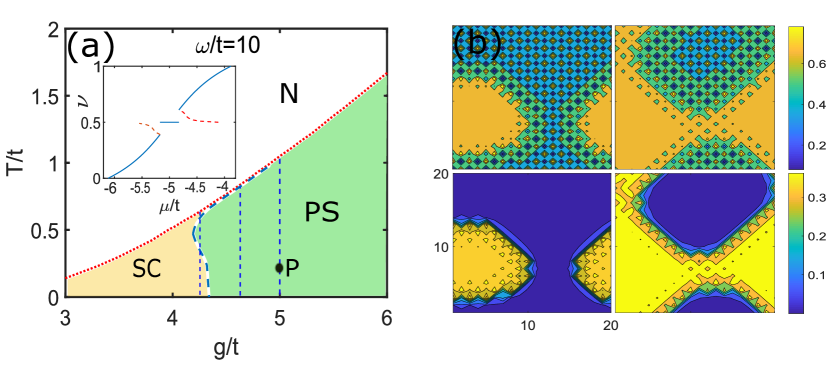
Figure 1: (a) Phase diagrams for the Holstein model in a $50\times 50$ lattice for $\omega_{b}/t=10$ and $\nu=0.6$. The inset displays the filling factor, $\nu$, as a function of the chemical potential at the point $P$, where $g/t=5$, $T/t=0.2$. (b) Phase separations at $P$ for $\nu=0.56$ (left panel) and $\nu=0.6$ (right panel) in a $20\times 20$ lattice. The first and second rows display the electron density and the SC order parameter.

Regarding the choice of variational states, a particularly useful set for the zero temperature case was introduced in Tao , and consists of states in the form

$$|\Psi(\xi)\rangle=U(\xi_{u})|\Psi_{G}(\xi_{g})\rangle.$$ (2)

Here, $\xi=(\xi_{u},\xi_{g})$ contains the variational parameters, $U\in\mathcal{U}$, a set of unitary operators with a special form, and $\Psi_{G}$ is an arbitrary Gaussian state. The latter are those which can be written in terms of a Gaussian function of creation and annihilation operators, and they are very versatile as they can be fully characterized in terms of the so-called covariance matrix and displacement vector (for the case of bosons) QO ; FG . Furthermore, $U$ is non-Gaussian, so that it can encompass different phenomena; in particular, in case one has both fermions and bosons, it can describe non-trivial correlations among them, something which is absent in Gaussian states. The TDVP method based on states of the form (2) has been successfully applied to several problems. Those include the Holstein and SSH models Tao , polaron and spin-boson problems Tao ; Ultrastrong , Kondo and Anderson impurity models Kondo ; Anderson ; Rydberg , the 2D Hubbard-Holstein model Hubbard_Holstein , and the Schwinger-like models with non-abelian gauge groups LGT .

In this Letter, we introduce a free energy flow based variational method (FEFVM) to study systems at finite temperature, and show how it can be applied to states of the form (2). Firstly, we derive an equation that extends parametric flow in (1) to finite temperatures, and which ensures that the free energy monotonically decreases during the flow, so that, regardless of the initial density operator, the system should ultimately flow to the Gibbs state. Secondly, we use a purification of that state to re-express such flow equation in the form similar to equation (1). And finally, following Tao , we show how to apply this flow based formalism to variational states of the form (2), obtaining a set of differential equations for $\xi(\tau)$, which ensure that the free energy decreases during the flow. Thus, the problem of studying finite temperature systems with FEFVM with such a family of states possesses the same complexity as the standard ITVM for zero temperature. We benchmark our method with the two dimensional (2D) negative-$U$ Hubbard model, for which standard mean-field theory can be easily applied, and show that it yields more reliable results than the ITVM. Then, we apply it to the 2D Holstein model, which describes electrons hopping on a lattice and interacting with phonons. In Fig. 1a, we present the resulting phase diagram for the phonon frequency $\omega_{b}/t=10$ and a filling factor $\nu=0.6$, where $T$ is the temperature, $g$ the coupling constant, and $t$ the hopping energy. As expected, our method predicts a superconducting phase at low $g$ (when the model reduces to the BCS). For higher values of $g$, it predicts separation between a auperconducting (SC) and a charge-density wave (CDW) phases. This is obtained by both, a homogeneous and a general variational ansatz. In the first case, this can be deduced from the dependence of the filling factor on the chemical potential (insert in Fig. 1a), whereas in the latter it explicitly follows from the distribution of the electron density and the SC order parameter (Fig. 1b). We point out that our approach predicts a CDW transition temperature that monotonically increases with increasing electron-phonon coupling strength. This temperature should be understood as the pseudogap temperature of the onset of short-range correlations. Our method is mean-field in its character and does not fully account for long-wavelength fluctuations of the order parameter that determine the actual Tc. We expect however that it accurately describes the increasing temperature of phase separation.

Imaginary time evolution for the Free energy: Given a Hamiltonian, $H$, and a temperature, $T$, we are interested in the Gibbs state described in terms of the density operator

$$\rho_{T}=\frac{e^{-\beta H}}{Z},$$ (3)

where $Z=\mathrm{tr}(e^{-\beta H})$ is the partition function, and $\beta=1/T$. A unique feature of such an operator is that it minimizes the free energy function

$$f(\rho)=\mathrm{tr}(H\rho)-TS(\rho),$$ (4)

where $S(\rho)=-\mathrm{tr}[\rho\ln(\rho)]$ is the von Neumann entropy of $\rho$. The minimum of $f$ with respect to all possible density operators is reached for $\rho=\rho_{T}$, so that this provides us with the variational principle to determine the Gibbs state. Here, we will show how this minimization can be done through a differential equation, akin to the zero temperature state.

We define the free energy operator $F(\rho)=H+T\ln\rho$, so that $f(\rho)=\mathrm{tr}[\rho F(\rho)]$. Now, let us consider the following equation

$$d_{\tau}\rho=-\{F(\rho)-f(\rho),\rho\}.$$ (5)

We want to show that any initial (normalized) state, $\rho(0)$, flows to $\rho_{T}$. For that, we will show that $d_{\tau}f[\rho(\tau)]\leq 0$ with the equality holding only if $\rho=\rho_{T}$. From the definition of $f(\rho)$, we have $d_{\tau}f(\rho)=\mathrm{tr}(Fd_{\tau}\rho)+T\mathrm{tr}[\rho d_{\tau}\ln(\rho)]$. The last term vanishes, since $\mathrm{tr}[\rho d_{\tau}\ln(\rho)]=\mathrm{tr}\left[\int_{0}^{1}due^{(1-u)\ln(\rho)}d_{\tau}[\ln(\rho)]e^{u\ln(\rho)}\right]=\mathrm{tr}\left[d_{\tau}e^{\ln(\rho)}\right]=\mathrm{tr}(d_{\tau}\rho)=0$ where we have utilized that Eq. (5) conserves the trace of $\rho$. Using Eq. (5) we obtain

$$d_{\tau}f(\rho)=-2\mathrm{tr}\left[\rho X(\rho)^{2}\right]\leq 0,$$ (6)

where we have defined $X(\rho)=[F(\rho)-f(\rho)]$. The derivative vanishes when $X(\rho)=0$ which leads to (3) footnote2 . Note that while we refer to (5) as imaginary time flow, it does not correspond to the analytic continuation of the real time evolution of the density matrix, except for the case of zero temperature.

The last piece we need is to transform (5) into an equation analogous to (1). For that, we employ a particular purification of $\rho$, $\Phi_{p}$ (also called thermal double thermo ). This is done by adding for each (bosonic or fermionic) mode an auxiliary one so that

$$|\Phi_{p}\rangle=(\sqrt{\rho}\otimes{\openone})|\Phi^{+}\rangle$$ (7)

where $\Phi^{+}$ is a maximally entangled state between each mode and the corresponding ancilla, and thus fulfills $\mathrm{tr}_{a}[|\Phi^{+}\rangle\langle\Phi^{+}|)\propto{\openone}$ footnote3 . We can recover $\rho$ out of $\Phi_{p}$ by simply tracing out the ancillas, i.e., $\rho=\mathrm{tr}_{a}(|\Phi_{p}\rangle\langle\Phi_{p}|)$. It follows directly from (5) that

$$d_{t}|\Phi_{p}\rangle=-[F_{p}(\Phi_{p})-f_{p}(\Phi_{p})]|\Phi_{p}\rangle$$ (8)

where $F_{p}(\Phi)=F(\rho)\otimes{\openone}$ and $f_{p}(\Phi)=f(\rho)$, with $\rho=\mathrm{tr}_{a}(|\Phi\rangle\langle\Phi|)$. The similarity of Eqs. (8) and (1) is apparent, although the operator $F_{p}$ explicitly depends on the state $\Phi$ and only acts non-trivially on the system (and not on the ancillas). Thus, the resulting equation is non-linear.

Variational method: We are interested in approximating the Gibbs state (3) using the family of states

$$\rho_{v}(\xi)=U(\xi_{u})\rho_{G}(\xi_{g})U(\xi_{u})^{\dagger}.$$ (9)

In equation (9) $\rho_{G}$ in (9) is an arbitrary Gaussian mixed state parametrized by $\xi_{g}$ with $\mathrm{tr}(\rho_{G})=1$. $U$ is a unitary operator which entangles different degrees of freedom and allows us to describe states that do not obey Wick’s theorem of Gaussian ensembles. We consider the same family of unitary operators $U\in\mathcal{U}$ that has been defined in the zero temperature case in Ref. Tao , including all the conditions imposed on such operators. We assume that the number of variational parameters $\xi_{u}$ in $U$ scales polynomially with the system size. With the goal of describing states in (9) we consider states in the doubled space (physical + ancilla) of the form

$$|\Psi_{v}(\xi)\rangle=[U(\xi_{u})\otimes{\openone}]|\Psi_{G}(\xi_{g})\rangle$$ (10)

with a normalized pure Gaussian state $\Psi_{G}$ as the purification of $\rho_{v}(\xi)$, namely, $\rho_{v}(\xi)=\mathrm{tr}_{a}(|\Psi_{v}(\xi)\rangle\langle\Psi_{v}(\xi)|)$ as long as the trace over the auxiliary modes reproduces $\rho_{G}(\xi_{g})=\mathrm{tr}_{a}(|\Psi_{G}(\xi_{g})\rangle\langle\Psi_{G}(\xi_{g})|)$ . Note that in constructing the Gaussian state $\Psi_{G}$ we start with the maximally entangled state between the ancilla and physical degrees of freedom and then apply a Gaussian operator Tao that acts only on the physical degrees of freedom. Starting from Eq. (8) it is possible to derive a set of equations for variational parameters characterizing the purification. In SM we present details of such derivation and provide a simple proof that the free energy decreases in the course of parametric flow with $\tau$, as long as states have been chosen to be normalized. The method consists of projecting Eq. (8) onto the tangent plane of the manifold (10), in essentially the same way as it has been done for the zero temperature case. The set $\mathcal{U}$ should be chosen so that this can be done efficiently. Furthermore, a special feature of the chosen family of variational states is that the free energy operator, $F$, can be efficiently computed, since $\ln\rho_{v}=U(\xi_{u})\ln[\rho_{G}(\xi_{g})]U(\xi_{v})^{\dagger}$, and the logarithm of a Gaussian state can be readily calculated SM .

As variational parameters for the Gaussian state, $\xi_{g}$, we use the covariant matrix formalism. We consider a set of $N_{b}$ ($N_{f}$) bosonic (fermionic) with annihilation operators $b_{n}$ ($c_{m}$). For a Gaussian state we further define, as usual Tao ; QO ; FG ; SM , the covariance matrix $\Gamma_{b,m}$ for the bosons and fermions, respectively, and the displacement vector, $\Delta_{R}$ SM .

Some conserved quantities $O$, e.g., the particle number $O=N$, may commute with the many body Hamiltonian $H$. For the thermal state that breaks the symmetry, i.e., $[\rho,O]\neq 0$, we can fix the average value $\left\langle O\right\rangle$ in the flow equation by introducing a time-dependent Lagrangian multiplier, which allows us to compute the chemical potential SM .

Negative-U Hubbard Model: We first benchmark our method by analyzing this textbook model, and show how it overcomes some of the deficiencies of the ITVM. We consider the Hubbard Hamiltonian on a square lattice

$$H_{\mathrm{BCS}}=-t\sum_{\left\langle nm\right\rangle,\sigma}c_{n\sigma}^{\dagger}c_{m\sigma}+U\sum_{n}c_{n\uparrow}^{\dagger}c_{n\downarrow}^{\dagger}c_{n\downarrow}c_{n\uparrow},$$ (11)

where the first sum is restricted to nearest neighbors and $U<0$ describes attractive interactions. This is a well known Hamiltonian, where BCS theory correctly describes the appearance of a SC phase at sufficiently low temperatures. The mean-field approach to the BCS model is known to be quantitatively correct in the thermodynamic limit, although in one- and two-dimensional systems the transition temperature should be understood as that of opening of the quasi-particle gap, rather than the onset of the true long range order.

We compare the results of our method with the mean-field calculation and the ITVM mentioned in the introduction (see also SM ), and which is widely used, for instance, in the context of matrix product states pMPS . In both, the ITVM and the FEFVM, we use the Fermionic Gaussian family of translatinally invariant states (i.e., $(\Gamma_{m})_{{n,n^{\prime}}}=(\Gamma_{m})_{n-n^{\prime}}$). To account for the spontaneous symmetry breaking in the SC phase, in the ITVM we introduce a small symmetry breaking term in the Hamiltonian $\epsilon\sum_{n}c_{{n,\uparrow}}^{\dagger}c_{{n,\downarrow}}^{\dagger}$ and take $\epsilon\rightarrow 0$.

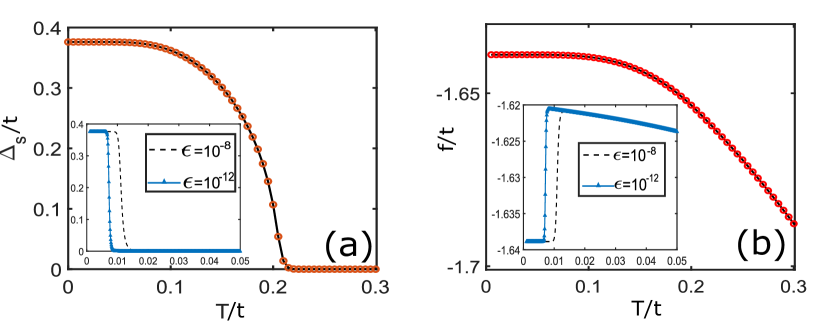
Figure 2: Lattice BCS Model: $s$-wave order parameter (a) and free energy density (b) as a function of the temperature $T/t$, for $U/t=-2$ and a $50\times 50$ lattice at half filling. The red curve gives the result of the FEFVM, which is on top of the mean field result in the thermodynamic limit. The black dashed line and the green curve (see insert) correspond to the ITVM for a symmetry-breaking field with $\epsilon=10^{-8},10^{-12}$, respectively.

The results are displayed in Fig. 2, where we draw the $s$-wave order parameter, $\Delta_{s}=U|\left\langle c_{n\downarrow}c_{n\uparrow}\right\rangle|$, as a function of the temperature at half filling. The figure shows that our method correctly reproduces the phase transition, whereas the one based on ITVM does not. As mentioned above, the accumulation of errors is responsible for this failure SM .

Holstein Model: We now investigate the 2D Holstein model, which describes electrons on a lattice interacting with optical phonons. The Hamiltonian is $H=H_{\mathrm{e}}+H_{\mathrm{ph}}+H_{\mathrm{int}}$, where $H_{\mathrm{e}}=-t\sum_{\left\langle n,m\right\rangle,\sigma}c_{n\sigma}^{\dagger}c_{m\sigma}$ and $H_{\mathrm{ph}}=\omega_{b}R^{T}R/4-\omega_{b}/2$, where $t$ and $\omega_{b}$ are the electron hopping and phonon frequency, respectively. The Holstein-type interaction $H_{\mathrm{int}}=g\sum_{n\sigma}x_{n}c_{n\sigma}^{\dagger}c_{n\sigma}$ between electrons and phonons is characterized by the coupling strength $g$. For weak electron phonon-interaction, $g\ll\omega_{b}$, one can eliminate the bosons and obtain the Hubbard model so that, at sufficient low temperatures, it displays an SC phase. For strong interactions and classical phonons, Esterlis et al. Esterlis have used a Monte-Carlo analysis to predict a commensurate CDW behavior that can be understood as the localized phase of bipolarons.

We use the variational Ansatz (10) with the generalized Lang-Firsov transformation $U=e^{S}$ Tao ; LangFirsov , where the generating function $S=i\sum_{ln,\sigma}\lambda_{ln}p_{l}c_{n\sigma}^{\dagger}c_{n\sigma}$ contains the variational parameters $\lambda_{ln}$. We use two different kinds of Ansaetze for $\Delta_{R}$, $\Gamma_{b,m}$, and $\lambda_{ln}$:

(i)

General, where all components of the vector $\Delta_{R}$ and matrices $\Gamma_{b}$, $\Gamma_{m}$, and $\lambda$ can take arbitrary values;

(ii)

Homogeneous, where $\Delta_{R,l}=\Delta_{R,0}+(-1)^{l}\Delta_{R,\pi}$ and $\xi_{n,n^{\prime}}=\xi_{0,n-n^{\prime}}+(-1)^{n}\xi_{\pi,n-n^{\prime}}$, with $\xi=\Gamma_{b},\Gamma_{m},\lambda$. Note that in this way we can describe not only states with translational symmetry, but also with CDW orders.

In both cases, the equations for the variational parameters can be easily established SM starting from (8).

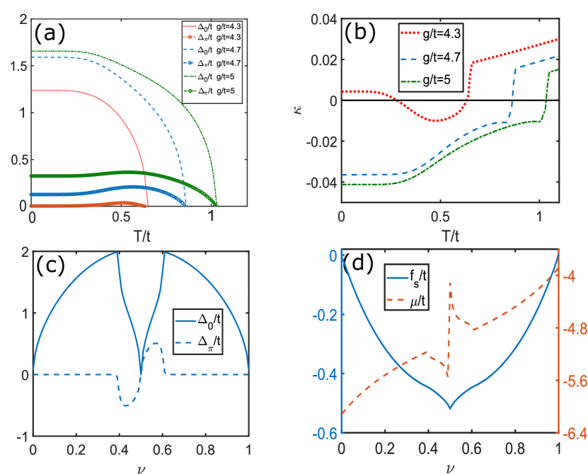
Figure 3: (a)-(b) The SC order parameters and the compressibility along three vertical lines in Fig. 1 obtained using homogeneous Ansaetze. Negative compressibility indicates thermodynamically unstable states and corresponds to phase separation. (c)-(d) The SC order parameters, the free energy, and the chemical potential versus the filling factor $\nu$ for $\omega_{b}/t=10$, $g/t=5$, $T/t=0.2$. All plots have been obtained with the homogeneous Ansatz.

In Fig. 1a, we show the phase diagram for the system with filling factor $\nu=0.6$ and $\omega_{b}/t=10$. As expected, for relatively small $g$ and low temperatures we find a SC phase. As $g$ increases, our method predicts phase separation between SC and a CDW phase. While the naive Ansatz (ii) predicts a supersolid phase (with non-vanishing SC and CDW order parameters), the general Ansatz (i) establishes phase separation, as it is shown in the snap-shots of Fig. 1b. One can recover this later behavior from (ii) as well by computing the chemical potential as a function of the filling factor $\nu$ (see insert in Fig. 1a). For $\nu$ in the interval $\sim[0.35,0.65]$ this analysis predicts phase separation between a CDW phase at half-filling, and a SC phase. The same result follows from Maxwell construction MC , in which one plots the free energy as a function of $\nu$ and draws straight lines that are tangent to the free energy $f$ and go through the minimum of $f$ (which occurs at half-filling). Maxwell construction allows to predict the fractions of CDW and SC phases for each value of the filling factor, $\nu$.

In Fig. 3a-b, we plot the order parameters $\Delta_{k=0,\pi}=\sum_{n}e^{-ikn}V_{nn}\left\langle c_{n\downarrow}c_{n\uparrow}\right\rangle/N$ and the compressibility $\kappa=\partial_{\nu}\mu$ for $g/t=4.3$, $4.7$, and $5$ as a function of the temperature (see also the three vertical lines in 1a), where $V_{nn}=2(\omega_{b}\sum_{l}\lambda_{ln}^{2}-2g\lambda_{nn})$ SM . A negative value indicates the onset of phase separation, which agrees with the corresponding region of phase diagram of Fig. 1. To carry out the Maxwell construction, in Fig. 3c-d, we display the order parameters $\Delta_{0,\pi}$, the free energy $f_{s}=f+4g^{2}\nu/\omega_{b}$ (extracting the phonon energy) and the chemical potential $\mu$ for $g/t=5$ and $T/t=0.2$ in a $50\times 50$ lattice. We have verified that this construction reproduces the results of the full variational Ansatz (i).

Spectral functions: Once we have obtained the variational approximation to the Gibbs state, we can also consider the evolution of the variational state in real time, which makes it possible to compute dynamical response functions or even analyze pump and probe experiments. Generally, one can consider situations when all parameters of the variational state in (9) become time dependent. However, when analyzing linear response it is often sufficient to keep parameters of the unitary transformation to be the same as in the equilibrium state and restrict the form of $\rho_{G}=U(\xi_{g})\rho_{0}U(\xi_{g})^{\dagger}$, so that the evolution does not change the spectrum of $\rho_{v}$. As one example of the dynamical response function, the electron spectral function measured in ARPES experiments can be calculated by extending the method reported in Anderson to finite temperature (see SM4).

Conclusions: We have developed a non-Gaussian variational approach to minimize the free energy of many-body systems at finite temperature. We have benchmarked it with the BCS and Holstein models. The later displays a transition between the SC phase for weak coupling and phase separated regime for stronger coupling. We find phase separation between the commensurate CDW at half filling and a SC phase with either lower or higher density, depending on whether the average density is below or above half-filling. Our findings are consistent with the results obtained by the Monte-Carlo analysis in the model with classical phonons Esterlis . Formalism developed in this paper can be extended to study broader classes of electron-phonon models, including the Migdal-Eliashberg regime with $\omega_{b}<t$, systems with both electron-electron and electron-phonon interactions, and systems with disorder.

Acknowledgements: We thank I. Esterlis and Y. Wang for stimulating discussions. T. S. acknowledges the Thousand-Youth-Talent Program of China. J.I.C acknowledges the ERC Advanced Grant QENOCOBA under the EU Horizon2020 program (grant agreement 742102) and the German Research Foundation (DFG) under Germany’s Excellence Strategy through Project No. EXC-2111-390814868 (MCQST) and within the D-A-CH Lead-Agency Agreement through project No. 414325145 (BEYOND C). ED acknowledges support from the Harvard-MIT CUA, Harvard-MPQ Center, AFOSR-MURI: Photonic Quantum Matter (award FA95501610323), and DARPA DRINQS program (award D18AC00014).

Supplemental Material

This supplemental material is divided into five sections. In Sec. SM1, we prove that the free energy decreases monotonically in the variational manifold as well. In Sec. SM2, we recall the definition of quadratures and covariance matrices for Gaussian states, and derive the explicit relation between the Gaussian thermal state and the corresponding covariance matrices. In Sec. SM3 we introduce a method to fix the expectation value of any operator $O$ commuting with the Hamiltonian in the flow equation. In Sec. SM4, we review the conventional purification methods to describe the time evolution in real and imaginary time. The first give rise to the ITVM mentioned in the text. As an application of the first, we give a technique to compute spectral functions. In Sec. SM5, for the Holstein model, we derove the equations of motion (EOM) for the parameters in the variational state, including a generalized Lang-Firsov transformation.

SM1 SM1. Monotonicity of the Free Energy in the FEFVM

In this section we show that the evolution equations for the variational parameters, $\xi=\{\xi_{j}\}$, ensure that the free energy decreases monotonically with time so long as the states $\Psi(\xi)$ in the variational family are normalized, that is, if we choose

$$\langle\Psi(\xi)|\Psi(\xi)\rangle=1$$ (SM1)

for all values of $\xi$. For that, let us first write the equation for the variational state as

$$d_{\tau}|\Psi(\xi)\rangle=-\mathbb{P}[\xi(\tau)]\left(F\{\rho[\xi(\tau)]\}\otimes\mathbb{I}-f\{\rho[\xi(\tau)]\}\mathbb{I}\otimes\mathbb{I}\right)|\Psi[\xi(\tau)]\rangle.$$ (SM2)

In the following, in order to simplify the notation, we will not write explicitly the dependence of the states and operators on $\xi$, the tensor product, nor the identity operators. In (SM2), $\rho=\mathrm{tr}_{a}(|\Psi\rangle\langle\Psi|)$ is the reduced state, $f(\rho)$ defined in Eq. (4), $F(\rho)=H+T\ln\rho$, and $\mathbb{P}$ is the projector onto the tangential subspace spanned by $\partial_{\xi_{j}}|\Psi(\xi)\rangle$.

The normalization condition (SM1) implies

$$0=d_{\tau}\langle\Psi|\Psi\rangle=\langle(F\mathbb{P}+\mathbb{P}F)\rangle-2f\langle\mathbb{P}\rangle$$ (SM3)

where we have written $\langle\ldots\rangle=\langle\Psi|\ldots|\Psi\rangle$. Thus, we have

$$d_{\tau}f=d_{\tau}\langle F\rangle=f\langle(F\mathbb{P}+\mathbb{P}F)\rangle-2\langle F\mathbb{P}F\rangle=-2\langle(F-f)\mathbb{P}(F-f)\rangle\leq 0$$ (SM4)

where we have used (SM3) and the fact that for any operator $X$, $X\mathbb{P}X^{\dagger}$ is positive semi-definite. We have also utilized that

$$\langle d_{\tau}F\rangle=\mathrm{tr}(d_{\tau}\rho)=0.$$ (SM5)

Therefore, as announced, the free energy of the variational state decreases under the FEFVM.

SM2 SM2. Gaussian thermal states

We define quadrature (Majorana) operators $x_{n}=b_{n}+b_{n}^{\dagger}$, $p_{n}=i(b_{n}^{\dagger}-b_{n})$ for the bosons [$a_{1,n}=c_{n}+c_{n}^{\dagger}$, $a_{2,n}=i(c_{n}^{\dagger}-c_{n})$ for the fermions]. We collect these operators in column vectors $R=(x_{1},\ldots,p_{1},\ldots)^{T}$ and $A=(a_{1,1},\ldots,a_{2,1},\ldots)^{T}$. The Gaussian state is characterized by the quadrature and covariance matrices

$$\Delta_{R} = \langle\Psi_{G}|R|\Psi_{G}\rangle,$$ (SM6a)

$$\Gamma_{b} = \frac{1}{2}\langle\Psi_{G}|\{\tilde{R},\tilde{R}^{T}\}|\Psi_{G}\rangle,$$ (SM6b)

$$\Gamma_{m} = \frac{i}{2}\langle\Psi_{G}|[A,A^{T}]|\Psi_{G}\rangle,$$ (SM6c)

where $$\tilde{R}=R-\Delta_{R}$$ is the fluctuation around the average value.

We parametrize the Gaussian density matrix $\rho_{G}=e^{-K}/Z$ by

$$K = \frac{1}{4}\tilde{R}^{T}\Omega_{b}\tilde{R}+i\frac{1}{4}A^{T}\Omega_{m}A$$ (SM7)

$$= \frac{1}{4}\tilde{R}^{T}\Omega_{b}\tilde{R}+\frac{1}{2}C^{\dagger}\Omega_{f}C$$

with the matrices $\Omega_{b}$ and $\Omega_{m}$ (or $\Omega_{f}=iW^{\dagger}\Omega_{m}W/2$ in the Nambu basis $C=(c,c^{\dagger})^{T}$), where the partition function $Z=\mathrm{tr}(e^{-K})$. We introduce the unitary operators $U_{K}$ that transforms $\tilde{R}$ and $C$ as $U_{K}^{\dagger}RU_{K}=\bar{S}_{b}R+\Delta_{R}$ and $U_{K}^{\dagger}CU_{K}=\bar{U}_{f}C$, where the symplectic matrix $\bar{S}_{b}$ and the unitary matrix $\bar{U}_{f}$ diagonalize $\Omega_{b}$ and $\Omega_{f}$, i.e., $\bar{S}_{b}^{T}\Omega_{b}\bar{S}_{b}=D_{b}$ and $\bar{U}_{f}^{\dagger}\Omega_{b}\bar{U}_{f}=E_{f}$.

By definition, the covariance matrices are

$$\Gamma_{b}=\frac{1}{2}\langle\Psi_{G}|\{\tilde{R},\tilde{R}^{T}\}|\Psi_{G}\rangle=\bar{S}_{b}\frac{1}{2}tr(\bar{\rho}_{G}\{R,R^{T}\})\bar{S}_{b}^{T}=\bar{S}_{b}\coth(\frac{D_{b}}{2})\bar{S}_{b}^{T},$$ (SM8)

and

$$\Gamma_{f}=\langle\Psi_{G}|CC^{\dagger}|\Psi_{G}\rangle=\bar{U}_{f}\frac{1}{e^{-E_{f}}+1}\bar{U}_{f}^{\dagger}=\frac{1}{e^{-\Omega_{f}}+1},$$ (SM9)

where we have used the property that the density matrix $\bar{\rho}_{G}=U_{K}^{\dagger}\rho_{G}U_{K}$ describes the thermal state of free bosons and fermions.

Using the symplectic property $\bar{S}_{b}\Sigma^{y}\bar{S}_{b}^{T}=\Sigma^{y}$ and the fact that $\coth(x/2)$ is an odd function, we can re-express $\Gamma_{b}$ in the compact form

$$\Gamma_{b}=\frac{e^{\Sigma^{y}\Omega_{b}}+1}{e^{\Sigma^{y}\Omega_{b}}-1}\Sigma^{y},$$ (SM10)

where $\Sigma^{y}=I_{N_{b}}\otimes\sigma^{y}$ is determined by the Pauli matrix $\sigma^{y}$. By inverting Eqs. (SM9) and (SM10), we obtain

$$\Omega_{b}=\Sigma^{y}\ln\frac{\Gamma_{b}\Sigma^{y}+1}{\Gamma_{b}\Sigma^{y}-1},$$ (SM11)

and

$$\Omega_{m}=i\ln(\frac{1+i\Gamma_{m}}{1-i\Gamma_{m}}).$$ (SM12)

SM3 SM3. Conserved quantities under the FEFVM

For a system with a conserved quantity $O$, i.e., $[O,H]=0$, the thermal state may break that symmetry, i.e., $[O,\rho]\neq 0$. A typical example is the $U(1)$ symmetry breaking in superconductors, where the total fermion number operator $N$ commutes with the Hamiltonian, however, the thermal state breaks that symmetry. In this section, we introduce a time-dependent term in the flow equation to fix the average value $\left\langle O\right\rangle$.

We modify the flow equation (8) to

$$\partial_{\tau}\left|\Psi\right\rangle=-\mathbf{P}_{O}(F-\mathcal{E})\left|\Psi\right\rangle,$$ (SM13)

where the projector

$$\mathbf{P}_{O}=1-\frac{1}{\mathcal{N}_{O}}O\left|\Psi\right\rangle\left\langle\Psi\right|O,$$ (SM14)

$\mathcal{N}_{O}=\left\langle\Psi\right|O^{2}\left|\Psi\right\rangle$, and $\mathcal{E}$ is a time dependent function to be determined. It immediately follows that Eq. (SM13) leads to the conservation law $\partial_{\tau}\left\langle O\right\rangle=0$.

To fulfill the normalization condition $\partial_{\tau}\left\langle\Psi\left|\Psi\right\rangle\right.=0$, we choose

$$\mathcal{E}=\frac{\left\langle F\right\rangle-\frac{1}{\mathcal{N}_{O}}\left\langle O\right\rangle\left\langle OF\right\rangle}{1-\frac{1}{\mathcal{N}_{O}}\left\langle O\right\rangle^{2}}.$$ (SM15)

A straightforward calculation results in

$$\partial_{\tau}\left|\Psi\right\rangle=-(\bar{F}-\left\langle\bar{F}\right\rangle)\left|\Psi\right\rangle,$$ (SM16)

where the new free energy operator $\bar{F}=F-\mu_{O}O$ is modified, with a time-dependent function

$$\mu_{O}=\frac{\left\langle OF\right\rangle-\left\langle O\right\rangle\left\langle F\right\rangle}{\mathcal{N}_{O}-\left\langle O\right\rangle^{2}},$$ (SM17)

For $O=N$,the particle number, $\mu_{O}$ is the chemical potential, which adjusts itself during the flow in order to keep the average value $\left\langle N\right\rangle$ unchanged. This equation can be projected onto the tangent plane of the variational manifold in order to obtain the differential equations for the variational parameters.

SM4 SM4. Imaginary and real time evolutions through purification

In the standard purification method, the thermal state $\rho_{T}=e^{-\beta H}/Z$ can be written as $\rho_{T}=\mathrm{tr}_{a}|\Phi_{p}\rangle\left\langle\Phi_{p}\right|$ with

$$|\Phi_{p}\rangle=\frac{1}{\sqrt{Z}}(e^{-\frac{1}{2}\beta H}\otimes{\openone})|\Phi^{+}\rangle,$$ (SM18)

or, in a more symmetric form, $\rho_{T}=\mathrm{tr}_{a}|\Phi_{s}\rangle\left\langle\Phi_{s}\right|$ with

$$|\Phi_{s}\rangle=\frac{1}{\sqrt{Z}}(e^{-\frac{1}{4}\beta H}\otimes e^{-\frac{1}{4}\beta\bar{H}})|\Phi^{+}\rangle,$$ (SM19)

where $|\Phi^{+}\rangle$ is the maximal entangled state.

For bosons, the Hamiltonian of the ancillas is $\bar{H}=H^{T}$. For fermions, we notice the relation

$$c|\Phi^{+}\rangle=d^{\dagger}|\Phi^{+}\rangle,c^{\dagger}|\Phi^{+}\rangle=-d|\Phi^{+}\rangle$$ (SM20)

for the annihilation and creation operators of the system and ancillas acting on $|\Phi^{+}\rangle=(1+c^{\dagger}d^{\dagger})|0\rangle/\sqrt{2}$. As a result, one has to add a minus sign for the creation operator, corresponding to a particle-hole transformation between system and ancilla.

Let us consider now the imaginary time evolution dictated by a Hamiltonian $H$. The EOM for $|\Phi_{p}\rangle$ and $|\Phi_{s}\rangle$ are

$$\partial_{\tau}|\Phi_{p}\rangle=-\frac{1}{2}(H\otimes{\openone}-\left\langle H\right\rangle)|\Phi_{p}\rangle$$ (SM21)

and

$$\partial_{\tau}|\Phi_{s}\rangle=-\frac{1}{4}(H\otimes{\openone+\openone}\otimes H-2\left\langle H\right\rangle)|\Phi_{s}\rangle.$$ (SM22)

The thermal Gibbs state is obtained by evolving this state starting from $\Phi^{+}$ for a time $\tau=\beta/2$. One can project this equation onto the tangent plane of any variational manifold in order to obtain a practicable method to study thermal equilibrium, which leads to the ITVM as described in the main text.

The standard purification method works very well if the solutions $|\Phi_{p,s}\rangle$ are exact; however, it may not give reliable results for variational states. One can track the reason for the potential failure of this method as follows. First, the standard method accumulates error along the time evolution up to the time $\tau=\beta/2$. The FEFVM, however, obtains the purified state at a fixed point, $\tau\rightarrow\infty$, and thus it does not depend on the path used to reach it. For the ITVM, this can be seen very clearly as follows in the BCS model described in the main text. Since we are dealing with Gaussian states, the projection onto the tangent plane can be translated into a differential equation of the form $d_{\tau}|\Psi_{G}\rangle=-H_{\mathrm{P}}(\tau)|\Psi_{G}\rangle$, where the projected Hamiltonian depends on the variational parameters and is thus time dependent. The solution to this equation can be written as $|\Psi(\tau)\rangle\propto\mathcal{T}\exp[-\int_{0}^{\tau}d\tau^{\prime}H_{\mathrm{P}}(\tau^{\prime})]|\Phi^{+}\rangle$, whereas we know that state that minimizes the free energy must have a purification of the form $|\Psi(\tau)\rangle\propto\exp[-H_{\mathrm{eff}}(\tau)]|\Phi^{+}\rangle$. Furthermore, the ITVM does not perform well whenever there is symmetry breaking. Since the initial thermal state with infinite temperature maintains all the symmetries, one has to add a small symmetry breaking term in the Hamiltonian. However, the appearance of the symmetry breaking is very sensitive to that term, and the corresponding order parameter only agrees with that from the correct BCS theory near zero temperature.

Let us now move to the variational study of real time evolution of mixed states. In this case, the density matrix $\rho$ obeys the Liouville equation

$$i\partial_{t}\rho=[H,\rho],$$ (SM23)

where in general $\rho$ can be a mixed state. We introduce the purification for $\rho=\mathrm{tr}_{a}|\Phi_{p}\rangle\left\langle\Phi_{p}\right|$, where

$$|\Phi_{p}\rangle=(\sqrt{\rho}\otimes{\openone})|\Phi^{+}\rangle.$$ (SM24)

One can easily show that the Schrödinger equation

$$i\partial_{t}|\Phi_{p}\rangle=H\otimes{\openone}|\Phi_{p}\rangle$$ (SM25)

leads to Eq. (SM23). The Eq. (SM25) can then be solved variationally Tao .

The purified Schrödinger Eq. (SM25) can be applied to study the spectral function $A(\omega)=-$Im$G_{R}(\omega)/\pi$, where $G_{R}(\omega)$ is the Fourier transformation of the retarded Green function

$$G_{R}(t)=-itr\rho\{c(t),c^{\dagger}\}\theta(t)$$ (SM26)

defined in some basis $c=(c_{1},c_{2},...,c_{N})^{T}$. By the purification, the Green function becomes

$$G_{R}(t) = -i\left\langle\Phi_{p}\right|\{c(t),c^{\dagger}\}|\Phi_{p}\rangle\theta(t)$$ (SM27)

$$= -i\left\langle\Phi_{p}\right|e^{iHt}ce^{-iHt}c^{\dagger}|\Phi_{p}\rangle\theta(t)-i\left\langle\Phi_{p}\right|c^{\dagger}e^{iHt}ce^{-iHt}|\Phi_{p}\rangle\theta(t).$$

By taking the second term in Eq. (SM27) as an example, we first calculate the real-time evolution $|\Phi_{p}(t)\rangle=e^{-iHt}|\Phi_{p}\rangle$ by using Eq. (SM25). The second real-time evolution $|\bar{\Phi}_{p}(t)\rangle=e^{iHt}(c|\Phi_{p}(t)\rangle)$ can also be obtain by solving Eq. (SM25), where the Hamiltonian $H$ is replaced by $-H$. Finally, the second term in Eq. (SM27) becomes the overlap $-i\left\langle\Phi_{p}\right|c^{\dagger}|\bar{\Phi}_{p}(t)\rangle$.

In practice, one has to carefully choose the variational manifold $\mathcal{M}$, such that $\{|\Phi_{p}\rangle$, $c|\Phi_{p}(t)\rangle$, $|\bar{\Phi}_{p}(t)\rangle\}\in\mathcal{M}$ and the overlap $-i\left\langle\Phi_{p}\right|c^{\dagger}|\bar{\Phi}_{p}(t)\rangle$ can be evaluated efficiently. The Gaussian variational manifold satisfies this condition, where Eq. (SM25) is projected in the Gaussian manifold. It is worthy to remark that the time-dependent global phase in the real time evolution is crucial for the spectral function, which can be tracked by the Wei-Norman algebra method Tao .

A further approximation can be applied to simplify the calculation of $A(\omega)$. The Hamiltonian $H$ in Eq. (SM27) can be approximated by the mean-field Hamiltonian $H_{\mathrm{MF}}=C^{\dagger}\mathcal{H}_{f}C/2$ in the Nambu basis $C=(c,c^{\dagger})$ Anderson , where $\mathcal{H}_{f}$ is constructed in the equilibrium state by the Wick theorem, similarly to the treatment in the superconductivity theory. As a result, the Green function $G_{R}(t)=-ie^{-i\mathcal{H}_{f}t}\theta(t)$, and the spectral function $A(\omega)=\delta(\omega-\mathcal{H}_{f})$ displays the peaks corresponding to the quasi-particle energy. In the electron-phonon interacting system, the phonon broadening effects in the spectral function can be included by the expansion of $H=H_{\mathrm{MF}}+H_{I}$ in the vicinity of the Gaussian thermal state $\rho$, where the mean-field Hamiltonian $H_{\mathrm{MF}}$ has the quadratic form and $H_{I}$ contains the higher order terms. The perturbation theory gives rise to the renormalization of the quasi-particle energy and the broadening of the peak in $A(\omega)$.

SM5 SM5. Application to Holstein models

We derive the EOM of $\Delta_{R}$, $\Gamma_{b,m}$, and $\lambda_{ln}$ for the Holstein model by projecting Eq. (8) on the tangential space. The tangential vextor of the variational ansatz (10) determined by the Lang-Firsov transformation $U=e^{S}$ reads

$$d_{\tau}|\Psi_{v}\rangle=e^{S}[i\sum_{ln,\sigma}d_{\tau}\lambda_{ln}p_{l}c_{n\sigma}^{\dagger}c_{n\sigma}|\Psi_{G}\rangle+d_{\tau}|\Psi_{G}\rangle]$$ (SM28)

The Gaussian state $|\Psi_{G}\rangle=U_{\mathrm{GS}}|0\rangle$ is determined by the unitary operator $U_{\mathrm{GS}}$ that transforms $C$ and $R$ as $U_{\mathrm{GS}}^{\dagger}RU_{\mathrm{GS}}=\Delta_{R}+S_{b}R$ and $U_{\mathrm{GS}}^{\dagger}CU_{\mathrm{GS}}=U_{f}C$, where $S_{b}$ and $U_{f}$ are the time-dependent symplectic and unitary matrices.

The time derivative to $|\Psi_{G}\rangle$ gives rise to the tangential vector $d_{\tau}|\Psi_{v}\rangle=e^{S}U_{\mathrm{GS}}(|V_{1}\rangle+|V_{2}\rangle+|V_{3}\rangle)$. The tangential vector $|V_{1}\rangle=-R^{T}S^{T}\xi_{1}|0\rangle/2$ containing the linear operator is determined by

$$\xi_{1}=\Sigma^{y}d_{\tau}\Delta_{R}-2i\sum_{n\sigma}d_{\tau}\lambda_{ln}\left\langle c_{n\sigma}^{\dagger}c_{n\sigma}\right\rangle.$$ (SM29)

The tangential vector

$$|V_{2}\rangle=\text{:}[-\frac{1}{4}R^{T}S_{b}^{T}\Sigma^{y}d_{\tau}S_{b}R+\frac{1}{2}C^{\dagger}U_{f}^{\dagger}(d_{\tau}+O_{f})U_{f}C]\text{:}|0\rangle$$ (SM30)

contains the quadratic normal ordered operators acting on the vacuum state, where the anti-Hermitian matrix $O_{f}=\sigma^{z}\otimes I_{2}\otimes diag(i\sum_{l}\left\langle p_{l}\right\rangle d_{\tau}\lambda_{ln})$. The tangential vector

$$|V_{3}\rangle=i\sum_{ln,\sigma}(R^{T}S^{T})_{l}d_{\tau}\lambda_{ln}\text{:}U_{\mathrm{GS}}^{\dagger}c_{n\sigma}^{\dagger}c_{n\sigma}U_{\mathrm{GS}}\text{:}|0\rangle$$ (SM31)

contains the cubic normal ordered operators.

The right hand side of Eq. (8) can be written as

$$|V_{R}\rangle=-e^{S}[\bar{H}+T\ln\rho_{G}-f(\rho)]U_{\mathrm{GS}}|0\rangle,$$ (SM32)

where

$$\bar{H} = -t\sum_{\left\langle nm\right\rangle,\sigma}e^{-i\sum_{l}p_{l}(\lambda_{ln}-\lambda_{lm})}c_{n\sigma}^{\dagger}c_{m\sigma}-\mu\sum_{n\sigma}c_{n\sigma}^{\dagger}c_{n\sigma}+\frac{1}{4}\omega_{b}R^{T}R-\frac{1}{2}\omega_{b}$$ (SM33)

$$+\sum_{ln,\sigma}R_{l}^{T}G_{ln}c_{n\sigma}^{\dagger}c_{n\sigma}+\frac{1}{2}\sum_{n\sigma,m\sigma^{\prime}}V_{nm}c_{n\sigma}^{\dagger}c_{n\sigma}c_{m\sigma^{\prime}}^{\dagger}c_{m\sigma^{\prime}}$$

is determined by the renormalized electron-phonon interaction $G_{ln}=\left(g\delta_{ln}-\omega_{b}\lambda_{ln},0\right)^{T}$ and the electron-electron interaction

$$V_{nm}=2[\omega_{b}\sum_{l}\lambda_{ln}\lambda_{lm}-g(\lambda_{nm}+\lambda_{mn})]$$ (SM34)

induced by mediating phonons.

In the state $|V_{R}\rangle$, we can move the Gaussian unitary operator $U_{\mathrm{GS}}$ to the left side of the free energy operator, and obtain the vector $|V_{R}\rangle=-e^{S}U_{\mathrm{GS}}(|R_{1}\rangle+|R_{2}\rangle+|R_{3}\rangle)$. The linear vector reads

$$|R_{1}\rangle = [\frac{1}{2}\omega_{b}R^{T}S^{T}\Delta_{R}+\sum_{ln,\sigma}(R^{T}S^{T})_{l}G_{ln}\left\langle c_{n\sigma}^{\dagger}c_{n\sigma}\right\rangle$$ (SM35)

$$+i\sum_{\left\langle nm\right\rangle,\sigma}t_{\mathrm{eff},nm}(R^{T}S^{T})_{l}(\lambda_{ln}-\lambda_{lm})\left\langle c_{n\sigma}^{\dagger}c_{m\sigma}\right\rangle]|0\rangle,$$

where the renormalized hopping strength

$$t_{\mathrm{eff},nm}=te^{-i\sum_{l}\left\langle p\right\rangle_{l}(\lambda_{ln}-\lambda_{lm})}e^{-\frac{1}{2}w_{l,nm}\Gamma_{b,ll^{\prime}}w_{l^{\prime},nm}},$$ (SM36)

and $w_{l,nm}=\lambda_{ln}-\lambda_{lm}$.

The quadratic vector

$$|R_{2}\rangle=\frac{1}{4}R^{T}S^{T}\Omega_{\mathrm{MF}}SR+\frac{1}{2}C^{\dagger}U_{f}^{\dagger}\mathcal{F}_{f}U_{f}C$$ (SM37)

contains the bosonic and fermionic parts. The mean-field free energy $\Omega_{\mathrm{MF}}=\Omega_{0}-T\Omega_{b}$ of phonons is determined by

$$\Omega_{0}=\omega_{b}+2\sum_{\left\langle nm\right\rangle,\sigma}t_{\mathrm{eff},nm}\left\langle c_{n\sigma}^{\dagger}c_{m\sigma}\right\rangle w_{l,nm}w_{l^{\prime},nm}.$$ (SM38)

The mean-field free energy in the Dirac basis is $\mathcal{F}_{f}=\mathcal{H}_{f}-iW^{\dagger}T\Omega_{m}W/2$:

$$\mathcal{H}_{f}=\left(\begin{array}[]{cc}\mathcal{E}&\Delta\\ \Delta^{\dagger}&-\mathcal{E}^{T}\end{array}\right),$$ (SM39)

where the dispersion relation and effective chemical potential

$$\mathcal{E} = -t_{\mathrm{eff},nm}-V_{nm}\left\langle c_{m\sigma^{\prime}}^{\dagger}c_{n\sigma}\right\rangle-\mu_{\mathrm{eff,}n\sigma},$$ (SM40)

$$\mu_{\mathrm{eff,}n\sigma} = \mu-(\frac{1}{2}V_{nn}+\sum_{l}\Delta_{R,l}^{T}G_{ln})-\sum_{m\sigma^{\prime}}V_{nm}\left\langle c_{m\sigma^{\prime}}^{\dagger}c_{m\sigma^{\prime}}\right\rangle$$ (SM41)

of the phonon dressed polaron contains the Hartree-Fock corrections, and the gap matrix $\Delta_{n\sigma,m\sigma^{\prime}}=V_{nm}\left\langle c_{m\sigma^{\prime}}c_{n\sigma}\right\rangle$. The free energy of electrons in the Majorana basis is related to $\mathcal{F}_{f}$ as $\mathcal{F}_{m}=-iW\mathcal{F}_{f}W^{\dagger}/2$. The cubic vector is

$$|R_{3}\rangle=\sum_{l}(R^{T}S^{T})_{l}\text{:}U_{\mathrm{GS}}^{\dagger}[\sum_{\left\langle nm\right\rangle,\sigma}it_{\mathrm{eff},nm}w_{l,nm}c_{n\sigma}^{\dagger}c_{m\sigma}+\sum_{n\sigma}G_{ln}c_{n\sigma}^{\dagger}c_{n\sigma}]U_{\mathrm{GS}}\text{:}.$$ (SM42)

The projection on the linear tangential vector gives rise to the EOM

$$d_{\tau}\Delta_{R} = -\Gamma_{b}[\omega_{b}\Delta_{R}+2\sum_{n\sigma}G_{ln}\left\langle c_{n\sigma}^{\dagger}c_{n\sigma}\right\rangle$$ (SM43)

$$+2i\sum_{\left\langle nm\right\rangle,\sigma}t_{\mathrm{eff},nm}(\lambda_{ln}-\lambda_{lm})\left\langle c_{n\sigma}^{\dagger}c_{m\sigma}\right\rangle]$$

$$+2i\Sigma^{y}\sum_{n\sigma}d_{\tau}\lambda_{ln}\left\langle c_{n\sigma}^{\dagger}c_{n\sigma}\right\rangle$$

for the quadrature $\Delta_{R}$. The projection on the quadratic tangential vector results in the EOM

$$d_{\tau}\Gamma_{b} = \Sigma^{y}\Omega_{\mathrm{MF}}\Sigma^{y}-\Gamma_{b}\Omega_{\mathrm{MF}}\Gamma_{b},$$ (SM44)

$$d_{\tau}\Gamma_{f} = \{\Gamma_{f},\mathcal{F}_{f}\}-2\Gamma_{f}\mathcal{F}_{f}\Gamma_{f}+[\Gamma_{f},O_{f}]$$ (SM45)

for the covariance matrices $\Gamma_{b}$ and $\Gamma_{f}=1/2-iW^{\dagger}\Gamma_{m}W/4$.

The projection on the cubic tangential vector leads to

$$d_{\tau}\lambda_{ln}=\sum_{l^{\prime}}(\Gamma_{b,p}^{-1})_{ll^{\prime}}G_{l^{\prime}n}+\sum_{m}v_{lm}D_{mn}^{-1},$$ (SM46)

where $v_{lm}=\sum_{\delta,\sigma}w_{l,m+\delta m}t_{\mathrm{eff},mm+\delta}$Re$\left\langle c_{m\sigma}^{\dagger}c_{m+\delta\sigma}\right\rangle$ and the connected correlation function

$$D_{nm}=\sum_{\sigma\sigma^{\prime}}\left\langle c_{n\sigma}^{\dagger}c_{n\sigma}c_{m\sigma^{\prime}}^{\dagger}c_{m\sigma^{\prime}}\right\rangle_{c}.$$ (SM47)

References

(1) J. Bardeen, L. Cooper, and J. R. Schriffer, Phys. Rev. 106, 162; ibid., 108, 1175 (1957).
(3) C. V. Kraus and J. I. Cirac, New J. Phys. 12,
113004 (2010).
(4) T. Shi, E. Demler, and J. I. Cirac, Annals of Physics 390, 245 (2018).
(5) Note that in principle this procedure may lead to the
flow stopping at a local rather than the global minimum. However, the
experience so far shows that this can be overcome by taking different
initial values for .
(6) M. A. Nielsen and I. L. Chuang, Quantum Computation and
Quantum Information. Cambridge University Press,
Cambridge (2000).
(7) P. Martin and J. Schwinger, Phys. Rev. 115, 1342
(1959); J. Schwinger, J. Math. Phys. 2, 407 (1961).
(8) D. Walls and G. Milburn, Quantum Optics. Springer,
Berlin (1994).
(9) K. E. Cahill and R. J. Glauber, Phys. Rev. A 59 1538
(1999).
(10) T. Shi, Y. Chang, J. J. García-Ripoll, Phys. Rev.
Lett. 120, 153602 (2018).
(11) Y. Ashida, T. Shi, M. C. Bañuls, J. I. Cirac, and E.
Demler, Phys. Rev. Lett. 121, 026805 (2018); Phys. Rev. B, 98, 024103 (2018).
(12) T. Shi, J. I. Cirac, and E. Demler, arXiv:1904.00932.
(13) Y. Ashida, T. Shi, R. Schmidt, H. R. Sadeghpour, J. I.
Cirac, and E. Demler, arXiv:1905.08523; 1905.09615.
(14) Y.Wang, I. Esterlis, T. Shi, J. I. Cirac, E.
Demler, arXiv:1910.01792
(15) P. Sala, T. Shi, S. Kühn, M. C. Bañuls, E. Demler, and
J. I. Cirac, Phys. Rev. D 98, 034505 (2018).
(16) Strictly speaking, this is the only solution as long as
we impose that has full rank.
(17) For the bosonic case, the state is not
normalizable. However, since we use the covariant matrix formalism, this
problem can be easily circumvented.
(18) See Supplemental Material.
(19) M. Zwolak and G. Vidal, Phys. Rev. Lett. 93, 207205
(2004); F. Verstraete, J. J. García-Ripoll, and J. I. Cirac, Phys. Rev.
Lett. 93, 207204 (2004).
(20) I. Esterlis, S. Kivelson, and D. Scalapino, Phys. Rev. B
99, 174516 (2019).
(21) I. G. Lang and Y. A. Firsov, Zh. Eksp. Teor. Fiz.
43, 1843 (1962).
(22) L. E. Reichl, A Modern Course in Statistical Physics
(4th Edition), New York, NY USA: Wiley-VCH (2016).

References

(1) T. Shi, E. Demler, and J. I. Cirac, Annals of Physics 390, 245 (2018).
(2) T. Shi, J. I. Cirac, and E. Demler, arXiv:1904.00932.