Anisotropic a posteriori error estimate for the Virtual Element Method

Abstract.

We derive an anisotropic a posteriori error estimate for the adaptive conforming Virtual Element approximation of a paradigmatic two-dimensional elliptic problem. In particular, we introduce a quasi-interpolant operator and exploit its approximation results to prove the reliability of the error indicator. We design and implement the corresponding adaptive polygonal anisotropic algorithm. Several numerical tests assess the superiority of the proposed algorithm in comparison with standard polygonal isotropic mesh refinement schemes.

Keywords: Virtual Element Method, anisotropy, a posteriori error analysis.

1. Introduction and Notation

In recent years, the numerical approximation of partial differential equations on computational meshes composed by arbitrarily-shaped polygonal/polyhedral (polytopal, for short) elements has been the subject of an intense research activity. Examples of polytopal element methods (POEMs) include the Mimetic Finite Difference method, the Polygonal Finite Element Method, the Polygonal Discontinuous Galerkin Finite Element Method, the Hybridizable Discontinuous Galerkin and Hybrid High-Order Methods, the Gradient Discretization method, the Finite Volume Method, the BEM-based FEM, the Weak Galerkin method and the Virtual Element method (VEM). For more details see the special issue [6] and the references therein.

The novelty and recent surge of interest in POEMs stems from their ability to describe a physical domain using not only standard shapes (triangles, tetrahedra, square, hexahedra,…) but also highly irregular and arbitrary geometries. This flexibility of essentially arbitrary polytopal meshes is naturally very attractive for designing adaptive algorithms based on mesh refinement (and derefinement/agglomeration) driven by suitable a posteriori error estimates. However, while (isotropic and anisotropic) error estimates and a posteriori error estimates and adaptive finite element methods (AFEMs) have been intensively investigated during the last decades (see, e.g., for the isotropic case the monographs [32, 31] and the references therein and for the anisotropic case [4, 21, 22, 23, 24, 25, 26] and the references therein), the corresponding study of a posteriori error estimates and adaptivity for polytopal methods is still in its infancy. See, for example, [5, 8, 2] for the study of a posteriori error estimates in the context of Mimetic Finite Differences, [9, 13, 15, 29, 10, 19, 16] for the Virtual Element Method, [34, 35, 38, 37] for polygonal BEM-based FEM, [39] for the polygonal Discontinuous Galerkin method, [20] for the Mixed High Order method, [30] for the Weak Galerkin method and [33] for lowest-order locally conservative methods on polytopal meshes. Moreover, despite the great flexibility provided by polytopal meshes, the above works focused on the isotropic case, only. The anisotropic adaptive polytopal mesh refinement, to our knowledge, has been addressed only in [3] for the Virtual Element Method in two dimensions. For completeness, see also the recent work [17] for nonconforming VEM a priori anisotropic error analysis. Aim of this paper is to push forward the research of [3] providing a rigorous polygonal anisotropic a posteriori error estimate for conforming VEM and numerically assessing its efficacy in driving polygonal adaptive anisotropic mesh refinement strategies for the virtual element approximation of a paradigmatic two-dimensional elliptic problem.

The outline of the paper is as follows. In Section 2 we introduce the continuous elliptic problem together with its lowest order virtual element approximation. In Section 3 we first make precise the notion of polygonal anisotropy, then we state the anisotropic mesh regularity assumptions under which our theoretical results will be obtained. In the same section we also collect a series of instrumental results that will be employed in the subsequent analysis. In Section 4 we introduce a quasi-interpolant operator and prove approximation results that will be employed in Section 5 where a novel polygonal anisotropic a posteriori error estimate is obtained. Finally, in Section 6 we present a set of numerical results assessing the validity of our theoretical error estimates and the capability of our anisotropic error indicators to drive an adaptive polygonal anisotropic mesh refinement strategy for the solution of an elliptic problem.

1.1. Notation of functional spaces and technical results

We use the standard definition and notation of Sobolev spaces, norms and seminorms as given in [1]. Hence, the Sobolev space $H^{s}(\omega)$ consists of functions defined on the open bounded connected subset $\omega$ of $\mathbbm{R}^{2}$ that are square integrable and whose weak derivatives up to order $s$ are square integrable. As usual, if $s=0$, we prefer the notation $L^{2}(\omega)$. Norm and seminorm in $H^{s}(\omega)$ are denoted by $||\cdot||_{s,\omega}$ and $|\cdot|_{s,\omega}$, respectively, and $(\cdot,\cdot)_{\omega}$ denote the $L^{2}$-inner product. The subscript $\omega$ may be omitted when $\omega$ is the whole computational domain $\Omega$.

If $\ell\geq 0$ is an integer number, $\mathbbm{P}_{\ell}(\omega)$ is the space of polynomials of degree up to $\ell$ defined on $\omega$, with the convention that $\mathbbm{P}_{-1}(\omega)=\{0\}$. The $L^{2}$-orthogonal projection onto the polynomial space $\mathbbm{P}_{\ell}(\omega)$ is denoted by $\Pi^{0,\omega}_{\ell}\,:\,L^{2}(\omega)\to\mathbbm{P}_{\ell}(\omega)$. The space $\mathbbm{P}_{\ell}(\omega)$ is the span of the finite set of scaled monomials of degree up to $\ell$, that are given by

(1) $$\mathcal{M}_{\ell}(\omega)=\bigg{\{}\,\left(\frac{\mathbf{x}-\bar{\mathbf{x}}_{\omega}}{h_{\omega}}\right)^{\alpha}\textrm{~{}with~{}}|\alpha|\leq\ell\,\bigg{\}},$$

where

• $\bar{\mathbf{x}}_{\omega}$ denotes the center of gravity of $\omega$ and $h_{\omega}$ its characteristic length, as, for instance, the edge length or the cell diameter for $d=1,2$;

• $\alpha=(\alpha_{1},\alpha_{2})$ is the two-dimensional multi-index of nonnegative integers $\alpha_{i}$ with degree $|\alpha|=\alpha_{1}+\alpha_{2}\leq\ell$ and such that $\mathbf{x}^{\alpha}=x_{1}^{\alpha_{1}}x_{2}^{\alpha_{2}}$ for any $\mathbf{x}\in\mathbbm{R}^{2}$.

Finally, we use the symbols $\lesssim$ and $\gtrsim$ to denote inequalities holding up to a positive constant that is independent of the characteristic length of mesh elements, but may depend on the problem constants, like the coercivity and continuity constants, or other discretization constants like the mesh regularity constant, the stability constants, etc. Accordingly, $a\simeq b$ means $a\lesssim b\lesssim a$. The hidden constant generally has a different value at each occurrence.

2. Model problem and Virtual Element discretization

Let $\Omega\subset\mathbb{R}^{2}$ be a bounded polygonal domain. In this paper we are interested in deriving anisotropic error estimates for the virtual element approximation of the following elliptic problem:

(2) $$-\Delta u=f\quad\text{in~{}}\Omega,\qquad u=0\quad\text{on~{}}\partial\Omega$$

with $f\in L^{2}(\Omega)$. The variational formulation of (2) reads as: Find $u\in H^{1}_{0}(\Omega)$ such that

(3) $$a(u,v)=F(v)$$

for every $v\in H^{1}_{0}(\Omega)$ where $a(u,v)=\int_{\Omega}\nabla u\cdot\nabla v~{}d\mathbf{x}$ and $F(v)=\int_{\Omega}fv~{}d\mathbf{x}$.

We now briefly recall (see [11] for more details) the lowest order virtual element approximation to (3). Let $\{\mathcal{K}_{h}\}_{h}$ be a sequence of decompositions of $\Omega$ where each mesh $\mathcal{K}_{h}$ is a collection of nonoverlapping polygonal elements $K$ with boundary $\partial K$, and let $\mathcal{E}_{h}$ be the set of edges $E$ of $\mathcal{K}_{h}$. Each mesh is labeled by $h$, the diameter of the mesh, defined as usual by $h=\max_{E\in\mathcal{K}_{h}}h_{K}$, where $h_{K}=\sup_{\mathbf{x},\mathbf{y}\in K}|\mathbf{x}-\mathbf{y}|$. We denote the set of vertices ${\sf v}$ in $\mathcal{K}_{h}$ by $\mathcal{V}_{h}$. The global lowest order virtual element space is defined as

(4) $${\color[rgb]{0,0,0}V_{h,0}}=\{v_{h}\in H^{1}_{0}(\Omega):~{}v_{h}|_{K}\in V_{h}^{K}~{}\text{and~{}}v_{h}({\sf v})=0~{}\forall{\sf v}\in\partial\Omega\}\subset H^{1}_{0}(\Omega),$$

where

(5) $${\color[rgb]{0,0,0}V_{h}(K)}=\{v_{h}\in H^{1}(K):~{}\Delta v_{h}=0~{}\text{in}~{}K,~{}v_{h}|_{E}\in\mathbb{P}^{1}(E)~{}\forall E\subset\partial K\},$$

is the local virtual element space. We denote by $u_{h}\in{\color[rgb]{0,0,0}V_{h,0}}$ the virtual element approximation to the solution $u$ of (3), defined as the unique solution to

(6) $$a_{h}(u_{h},v_{h})=(f_{h},v_{h})$$

for every $v_{h}\in{\color[rgb]{0,0,0}V_{h,0}}$, where $f_{h}$ is the piecewise constant approximation of $f$ on $\mathcal{K}_{h}$ and $a_{h}(u_{h},v_{h})=\sum_{K\in\mathcal{K}_{h}}a^{K}_{h}(u_{h},v_{h})$ being

$$a^{K}_{h}(u_{h},v_{h})=\int_{K}{\color[rgb]{0,0,0}\Pi_{0}^{0,K}}\nabla(u_{h})\cdot{\color[rgb]{0,0,0}\Pi_{0}^{0,K}}\nabla(v_{h})~{}d\mathbf{x}+S^{K}((I-{\color[rgb]{0,0,0}\Pi_{1}^{0,K}})(u_{h}),(I-{\color[rgb]{0,0,0}\Pi_{1}^{0,K}})(v_{h})),$$

the local discrete bilinear form that satisfies the usual stability and consistency properties (see [11] for precise definitions). For $w_{h}\in\text{Ker}(\Pi_{1}^{0,K})$ the stabilization form $S^{K}(\cdot,\cdot)$ is defined as

$$S^{K}(w_{h},w_{h})=\sum_{i=1}^{n_{K}}w_{h}^{2}({\sf v}_{i,K}),$$

being ${\sf v}_{i,K}$, $i=1,\ldots,n_{K}$ the vertices of $K$. For more details about different choices for the stabilization form, see [7].

3. Polygonal Anisotropy and mesh regularity

In this section, following [36], we first make precise the notions of isotropic and anisotropic polygonal element. This will be obtained analysing the spectral decomposition of a suitable matrix ( in the sequel named covariance matrix) associated to the element. More precisely, let $K$ be a polygonal element of the partition $\mathcal{K}_{h}$. We denote by $|K|$ the area of $K$, we define the barycenter of $K$ as

$$\bar{\mathbf{x}}_{K}=\frac{1}{|K|}\int_{K}\mathbf{x}\,d\mathbf{x},$$

and we introduce the covariance matrix of $K$ as

(7) $$M_{\mathrm{Cov}}(K)=\frac{1}{|K|}\int_{K}(\mathbf{x}-\bar{\mathbf{x}}_{K})(\mathbf{x}-\bar{\mathbf{x}}_{K})^{\top}\,d\mathbf{x}\in\mathbb{R}^{2\times 2}.$$

Obviously, $M_{\mathrm{Cov}}$ is real valued, symmetric and positive definite, once we assume that $K$ is not degenerating (i.e. $|K|>0$). Therefore, $M_{\mathrm{Cov}}$ admits an eigenvalue decomposition

$$M_{\mathrm{Cov}}(K)=U_{K}\Lambda_{K}U_{K}^{\top},$$

with

(8) $$U^{\top}=U^{-1}\quad\mbox{and}\quad\Lambda_{K}=\operatorname{diag\,}(\lambda_{K,1},\lambda_{K,2}),$$

where $\lambda_{K,1}\geq\lambda_{K,2}>0$.

The eigenvectors of $M_{\mathrm{Cov}}(K)$ give the characteristic directions of $K$. Consequently, if

$$M_{\mathrm{Cov}}(K)=cI$$

for $c>0$, there are no dominant directions in the element $K$. Thus, we can characterise the anisotropy with the help of the quotient $\lambda_{K,1}/\lambda_{K,2}\geq 1$ and say that an element $K$ is

isotropic, if $$\frac{\lambda_{K,1}}{\lambda_{K,2}}\approx 1,$$

and anisotropic, if $$\frac{\lambda_{K,1}}{\lambda_{K,2}}\gg 1.$$

Hinging upon the above spectral informations on the polygonal elements, we introduce a linear transformation of an anisotropic element $K$ onto a kind of reference element $\widehat{K}$. For each $\mathbf{x}\in K$, we define the mapping by

(9) $$\mathbf{x}\mapsto\widehat{\mathbf{x}}=F_{K}(\mathbf{x})=A_{K}\mathbf{x}\quad\mbox{ with }\quad A_{K}=\alpha_{K}\Lambda_{K}^{-1/2}U_{K}^{\top}$$

where $\alpha_{K}>0$ will be chosen later. From now on, $\widehat{K}=F_{K}(K)$ will be called the reference element associated to $K$.

It is possible to prove (see [36]) the following result.

Lemma 3.1.

There holds

1. $|\widehat{K}|=\alpha_{K}^{2}|K|/\sqrt{\det(M_{\mathrm{Cov}}(K))}$,

2. $\overline{{\mathbf{x}}}_{\widehat{K}}=F_{K}(\overline{{\mathbf{x}}}_{K})$,

3. $M_{\mathrm{Cov}}(\widehat{K})=\alpha_{K}^{2}I$.

According to the previous lemma, the reference element $\widehat{K}$ is isotropic, since $\lambda_{\widehat{K},1}/\lambda_{\widehat{K},2}=1$, and thus, it has no dominant direction. For what concerns the choice of the parameter $\alpha_{K}$ we set

(10) $$\alpha_{K}=\left(\frac{\sqrt{\det(M_{\mathrm{Cov}}(K))}}{|K|}\right)^{1/d}=\left(\frac{\sqrt{\lambda_{K,1}\lambda_{K,2}}}{|K|}\right)^{1/2},$$

which obviously ensures, in view of Lemma 3.1, $|\widehat{K}|=1$. As usual, we mark the operators and functions defined over the reference configuration by a hat, as, for instance,

$$\widehat{v}=v\circ F_{K}^{-1}:\widehat{K}\to K.$$

Obviously, it is

(11) $$\nabla v=\alpha_{K}U_{K}\Lambda_{K}^{-1/2}\widehat{\nabla}\widehat{v},$$

and, after some algebra,

(12) $$\widehat{H}(\widehat{v})=\alpha_{K}^{-2}\Lambda_{K}^{1/2}U_{K}^{\top}H(v)U_{K}\Lambda_{K}^{1/2},$$

where $H(v)$ denotes the Hessian matrix of $v\in H^{2}(\Omega)$ and $\widehat{H}(\widehat{v})$ the corresponding Hessian on the reference configuration.

Following [36], we are now ready to state the mesh requirements which will be needed in the sequel for deriving the properties of the quasi-interpolation operator (Section 4) and the anisotropic a posteriori error analysis (Section 5). We first recall the notion of isotropic regular polygonal meshes (Definition 3.2) which is instrumental for the definition of anisotropic polygonal meshes (Definition 3.3).

Definition 3.2 (regular isotropic mesh).

A polygonal mesh $\mathcal{K}_{h}$ is called regular or a regular isotropic mesh, if all elements $K\in\mathcal{K}_{h}$ are such that:

1. $K$ is a star-shaped polygon with respect to a circle of radius $\rho_{K}$ and center $z_{K}\in K$.

2. The aspect ratio is uniformly bounded from above by $\sigma_{\mathcal{K}}$, i.e. $h_{K}/\rho_{K}<\sigma_{\mathcal{K}}$, being $h_{K}$ the diameter of $K$.

3. For every edge $E\subset\partial K$ it holds $h_{K}\leq c_{\mathcal{K}}h_{E}$, being $h_{E}$ the length of $E$.

Here, the constants $\sigma_{\mathcal{K}}$ and $c_{\mathcal{K}}$ have to be uniform for all considered regular elements.

Definition 3.3 (regular anisotropic mesh).

Let $\mathcal{K}_{h}$ be a polygonal mesh with anisotropic elements. $\mathcal{K}_{h}$ is called regular or a regular anisotropic mesh, if

1. The reference configuration $\widehat{K}$ for all $K\in\mathcal{K}_{h}$ obtained by (9) is a regular polygonal element according to Definition 3.2.

2. Neighbouring elements behave similarly in their anisotropy. More precisely, for two neighbouring elements $K^{+}$ and $K^{-}$, i.e. $\overline{K}^{+}\cap\overline{K}^{-}\neq\varnothing$, with covariance matrices

   $$M_{\mathrm{Cov}}(K^{+})=U_{K^{+}}\Lambda_{K^{+}}U_{K^{+}}^{\top}\quad\mbox{and}\quad M_{\mathrm{Cov}}(K^{-})=U_{K^{-}}\Lambda_{K^{-}}U_{K^{-}}^{\top}$$

   as defined above, we can write

   $$\Lambda_{K^{-}}=(I+\Delta^{K^{+},K^{-}})\Lambda_{K^{+}}\quad\mbox{with}\quad\Delta^{K^{+},K^{-}}=\operatorname{diag\,}\left(\delta^{K^{+},K^{-}}_{1},\delta^{K^{+},K^{-}}_{2}\right),$$

   and

   $$U_{K^{-}}=R^{K^{+},K^{-}}U_{K^{+}}\quad\mbox{with}\quad R^{K^{+},K^{-}}~{}\text{rotation~{}matrix}$$

   where for $i=1,2$

   $$0\leq|\delta^{K^{+},K^{-}}_{i}|<c_{\delta}<1\quad\mbox{and}\quad\|I-R^{K^{+},K^{-}}\|_{0}\left(\frac{\lambda_{K^{+},1}}{\lambda_{K^{+},2}}\right)^{1/2}<c_{\phi}.$$

   uniformly for all neighbouring elements, being $\|\cdot\|_{0}$ the spectral norm.

Thus a regular anisotropic element can be mapped according to (9) onto a regular polygonal element in the usual sense. In the definition of quasi-interpolation operators (see Section 4 ), we deal, however, with patches of elements instead of single elements. Thus, we study the mapping of such patches. Let $\omega=\omega_{\sf v}$ be the neighbourhood of the vertex ${\sf v}$ which is defined by

$$\overline{\omega}_{\sf v}=\bigcup\left\{\overline{K^{\prime}}:{\sf v}\in\overline{K^{\prime}},\quad K^{\prime}\in\mathcal{K}_{h}\right\}.$$

Furthermore, for $K\in\mathcal{K}_{h}$, recall that the map $F_{K}$ defined in  (9) is given by

$$\mathbf{x}\mapsto F_{K}(\mathbf{x})=A_{K}\mathbf{x}=\alpha_{K}\Lambda_{K}^{-1/2}U_{K}^{\top}\mathbf{x}.$$

Consequently, we may write $\widehat{K}=F_{K}(K)$ and we know, that $\widehat{K}$ is regular for all $K\in\mathcal{K}_{h}$ with some regularity parameters $\sigma_{\mathcal{K}}$ and $c_{\mathcal{K}}$. However, let now $K^{+},K^{-}\in\mathcal{K}_{h}$ with $K^{+},K^{-}\subset\omega$. We are interested in the regularity of $F_{K^{+}}(\omega)$ and $F_{K^{+}}(K^{-})$. For the proofs of the following results we refer to [36].

Lemma 3.4.

Let $\mathcal{K}_{h}$ be a regular anisotropic mesh, $\omega=\omega_{\sf v}$ be a patch as described above, and $K^{+},K^{-}\in\mathcal{K}_{h}$ with $K^{+},K^{-}\subset\omega$. The mapped element $F_{K^{+}}(K^{-})$ is regular in the sense of Definition 3.2 with slightly perturbed regularity parameters $\widetilde{\sigma}_{\mathcal{K}}$ and $\widetilde{c}_{\mathcal{K}}$. Consequently, the mapped patch $F_{K}(\omega)$ consists of regular polygonal elements for all $K\in\mathcal{K}_{h}$ with $K\subset\omega$.

Proposition 3.5.

Let $\mathcal{K}_{h}$ be a regular anisotropic mesh. Each vertex ${\sf v}$ of the mesh $\mathcal{K}_{h}$ belongs to a uniformly bounded number of elements. Viceversa, each element $K\in\mathcal{K}_{h}$ has a uniformly bounded number of vertices on its boundary.

In the rest of the paper we will work under the following mesh assumption.

Assumption 3.6.

Let $\{\mathcal{K}_{h}\}_{h}$ be a sequence of regular anisotropic meshes with regularity parameters uniformly bounded with respect to $h$.

Finally, we recall some instrumental results (see [36] for the proofs) that will employed in the next section.

Lemma 3.7.

Let $K\in\mathcal{K}_{h}$ be a polygonal element of a regular anisotropic mesh $\mathcal{K}_{h}$. Then, for $v\in H^{1}(K)$ and corresponding $\widehat{v}\in H^{1}(\widehat{K})$ there holds

(13) $$\|\widehat{v}\|_{L^{2}(\widehat{K})}=|K|^{-1/2}\|v\|_{L^{2}(K)}$$

(14) $$\|\widehat{\nabla}\widehat{v}\|_{L^{2}(\widehat{K})}=|K|^{-1/2}\|A_{K}^{-T}\nabla v\|_{L^{2}(K)}$$

(15) $$\sqrt{\frac{\lambda_{K,2}}{\lambda_{K,1}}}\;|\widehat{v}|_{H^{1}(\widehat{K})}^{2}\leq|v|_{H^{1}(K)}^{2}\leq\sqrt{\frac{\lambda_{K,1}}{\lambda_{K,2}}}\;|\widehat{v}|_{H^{1}(\widehat{K})}^{2}.$$

Lemma 3.8 (anisotropic trace inequality).

Let $K\in\mathcal{K}_{h}$ be a polygonal element of a regular anisotropic mesh $\mathcal{K}_{h}$. For an edge $E\subset\partial K$ it holds

(16) $$\|v\|_{L_{2}(E)}^{2}\lesssim\;\frac{|E|}{|K|}\left(\|v\|_{L_{2}(K)}^{2}+\|\alpha_{K}^{-1}\Lambda_{K}^{1/2}U_{K}^{\top}\nabla v\|_{L_{2}(K)}^{2}\right).$$

Lemma 3.9 (best-approximation by a constant).

Let $K\in\mathcal{K}_{h}$ be a polygonal element of a regular anisotropic mesh $\mathcal{K}_{h}$. For $v\in H^{1}(K)$, there exists a constant $p\in\mathcal{P}^{0}(K)$ such that

$$\|v-p\|_{L_{2}(K)}\lesssim\;\|\alpha_{K}^{-1}\Lambda_{K}^{1/2}U_{K}^{\top}\nabla v\|_{L_{2}(K)}.$$

4. Quasi-Interpolation of Functions in $H^{1}(\Omega)$

Let $\omega$ be a patch of physical elements belonging to a regular anisotropic polygonal mesh. Let $\widehat{\omega}$ be the patch of reference elements $\widehat{K}$ such that $\hat{\omega}=F_{K^{*}}(\omega)$, where the mapping is dictated by an element $K^{*}$ of the patch $\omega$. On the reference patch $\widehat{\omega}$ we introduce the space

(17) $$\widehat{\Theta}(\widehat{\omega})=\{\widehat{\theta}\in C^{0}(\widehat{\omega}):~{}\forall\widehat{K}\in\widehat{\omega}\,\,\widehat{\theta}_{|\widehat{K}}=\theta\circ F_{K^{*}}^{-1},~{}\theta\in V_{h}(F_{K^{*}}^{-1}(\widehat{K}))\}$$

where $V_{h}(F_{K^{*}}^{-1}(\widehat{K}))$ is the lowest order local virtual element space defined on the polygon $F_{K^{*}}^{-1}(\widehat{K})$. We remark that in view of Lemma 3.4 the specific choice of the element $K^{*}$ in the definition of the space $\widehat{\Theta}(\widehat{\omega})$ is not restrictive. Moreover, we observe that, in view of Assumption 3.6, the dimension of $\widehat{\Theta}(\widehat{\omega})$ is uniformly bounded with respect to $h$. Finally, it is worth noticing that functions in $\widehat{\Theta}(\widehat{\omega})$ are not necessarily virtual element functions. However, constant functions are contained in $\widehat{\Theta}(\widehat{\omega})$ and this will be sufficient for our scopes.

Now, following [12], we introduce a projection operator $\widehat{r}_{\omega}(\widehat{v})$ on the reference patch $\widehat{\omega}$.

Definition 4.1.

For any function $\widehat{v}\in L^{1}(\widehat{\omega})$ we define $\widehat{r}_{\omega}(\widehat{v})\in\widehat{\Theta}(\widehat{\omega})$ as

(18) $$\int_{\widehat{\omega}}(\widehat{r}_{\widehat{\omega}}(\widehat{v})-\widehat{v})\widehat{\theta}=0\qquad\forall\widehat{\theta}\in\widehat{\Theta}(\widehat{\omega}).$$

It is important to remark that $\widehat{r}_{\widehat{\omega}}$ is a projection operator on $\widehat{\omega}$.

On the physical patch $\omega$ we can define $r_{\omega}(v)$ so that $r_{\omega}(v)\circ F_{K^{*}}^{-1}=\widehat{r}_{\widehat{\omega}}(v\circ F_{K^{*}}^{-1})$, i.e. $\widehat{r_{\omega}(v)}=\widehat{r}_{\widehat{\omega}}(\widehat{v})$. Let $\omega_{i}$ be the patch of elements sharing the vertex $\sf{v}_{i}$ and set $r_{i}=r_{\omega_{i}}$. The operators $r_{i}$ will be employed to build the quasi-interpolant $\mathfrak{I}_{C}$ (see (23) below). In the sequel, we collect some approximation results for $r_{i}$ that will be instrumental for proving the approximation properties of $\mathfrak{I}_{C}$.

Lemma 4.2.

Let $\mathcal{K}_{h}$ be a regular anisotropic mesh. For any $K\subset\omega_{i}$ there hold

(19) $$\|u-r_{i}(u)\|^{2}_{L^{2}(K)}\lesssim\sum_{\widetilde{K}\subset\omega_{i}}\frac{|K|}{|\widetilde{K}|}\|A_{\widetilde{K}}^{-T}\nabla u\|^{2}_{L^{2}(\widetilde{K})}.$$

which can also be written in the following way

(20) $$\|u-r_{i}(u)\|^{2}_{L^{2}(K)}\lesssim|K|\sum_{\widetilde{K}\subset\omega_{i}}\sqrt{\frac{\lambda_{\widetilde{K},1}}{\lambda_{\widetilde{K},2}}}|u|^{2}_{H^{1}(\widetilde{K})}.$$

Proof.

Let $K\in\omega_{i}$ then we have

(21) $$\|u-r_{i}(u)\|_{L^{2}(K)} = |K|^{1/2}\|\widehat{u}-\widehat{r}_{\color[rgb]{0,0,0}\widehat{\omega}_{i}}(\widehat{u})\|_{L^{2}(\widehat{K})}.$$

Now, employing the fact that $\widehat{r}_{\color[rgb]{0,0,0}\widehat{\omega}_{i}}$ is a projector on $\widehat{\omega}_{i}$ we have

$$\widehat{u}-\widehat{r}_{\color[rgb]{0,0,0}\widehat{\omega}_{i}}(\widehat{u})=\widehat{u}-\widehat{\theta}-\widehat{r}_{\color[rgb]{0,0,0}\widehat{\omega}_{i}}(\widehat{u}-\widehat{\theta}),$$

for $\widehat{\theta}\in\widehat{\Theta}(\widehat{\omega}_{i})$ which implies

$$\|\widehat{u}-\widehat{r}_{\color[rgb]{0,0,0}\widehat{\omega}_{i}}(\widehat{u})\|_{L^{2}(\widehat{\omega}_{i})}\leq 2\|\widehat{u}-\widehat{\theta}\|_{L^{2}(\widehat{\omega}_{i})}.$$

Assume $\widehat{\theta}$ is constant on $\widehat{\omega}_{i}$ and $\widehat{u}\in H^{1}(\widehat{\omega}_{i})$, hence employing standard interpolation error estimate together with (14) we have

$$\|\widehat{u}-\widehat{r}_{\color[rgb]{0,0,0}\widehat{\omega}_{i}}(\widehat{u})\|_{L^{2}(\widehat{\omega}_{i})} \lesssim |\widehat{u}|_{H^{1}(\widehat{\omega}_{i})}$$

$$\lesssim \left(\sum_{\widehat{K}\subset\widehat{\omega}_{i}}|\widehat{u}|^{2}_{H^{1}(\widehat{K})}\right)^{1/2}$$

$$\lesssim \left(\sum_{\widetilde{K}\subset\omega_{i}}|\widetilde{K}|^{-1}\|A_{\widetilde{K}}^{-T}\nabla u\|^{2}_{L^{2}(\widetilde{K})}\right)^{1/2}.$$

Combining (21) with the above inequality yields (19). On the other hand, using (14)-(15) we get (20). ∎

Lemma 4.3.

For any $K\subset\omega_{i}$ there holds

(22) $$|u-r_{i}(u)|^{2}_{H^{1}(K)}\lesssim\sum_{\widetilde{K}\subset\omega_{i}}\sqrt{\frac{\lambda_{K,1}\lambda_{\widetilde{K},1}}{\lambda_{K,2}\lambda_{\widetilde{K},2}}}|u|^{2}_{H^{1}(\widetilde{K})}.$$

Proof.

By using (15) and taking $\widehat{\theta}$ constant on $\widehat{\omega}_{i}$, employing the equivalence of all norms on the finite dimensional space $\widehat{\Theta}(\widehat{\omega}_{i})$, the fact that $\widehat{r}_{\color[rgb]{0,0,0}\widehat{\omega}_{i}}$ is a projection on $\widehat{\omega}_{i}$ and standard interpolation error estimate we obtain

$$|u-r_{i}(u)|_{H^{1}(K)} \leq \left(\frac{\lambda_{K,1}}{\lambda_{K,2}}\right)^{1/4}|\widehat{u}-\widehat{r}_{\color[rgb]{0,0,0}\widehat{\omega}_{i}}(\widehat{u})|_{H^{1}(\widehat{K})}\leq\left(\frac{\lambda_{K,1}}{\lambda_{K,2}}\right)^{1/4}|\widehat{u}-\widehat{r}_{\color[rgb]{0,0,0}\widehat{\omega}_{i}}(\widehat{u})|_{H^{1}(\widehat{\omega}_{i})}$$

$$\leq \left(\frac{\lambda_{K,1}}{\lambda_{K,2}}\right)^{1/4}\left(|\widehat{u}-\widehat{\theta}|_{H^{1}(\widehat{\omega}_{i})}+|\widehat{\theta}-\widehat{r}_{\color[rgb]{0,0,0}\widehat{\omega}_{i}}(\widehat{u})|_{H^{1}(\widehat{\omega}_{i})}\right)$$

$$\lesssim \left(\frac{\lambda_{K,1}}{\lambda_{K,2}}\right)^{1/4}\left(|\widehat{u}-\widehat{\theta}|_{H^{1}(\widehat{\omega}_{i})}+\|\widehat{\theta}-\widehat{r}_{\color[rgb]{0,0,0}\widehat{\omega}_{i}}(\widehat{u})\|_{L^{2}(\widehat{\omega}_{i})}\right)$$

$$\lesssim \left(\frac{\lambda_{K,1}}{\lambda_{K,2}}\right)^{1/4}\left(|\widehat{u}-\widehat{\theta}|_{H^{1}(\widehat{\omega}_{i})}+\|\widehat{r}_{\color[rgb]{0,0,0}\widehat{\omega}_{i}}(\widehat{\theta}-\widehat{u})\|_{L^{2}(\widehat{\omega}_{i})}\right)$$

$$\lesssim \left(\frac{\lambda_{K,1}}{\lambda_{K,2}}\right)^{1/4}\left(|\widehat{u}-\widehat{\theta}|_{H^{1}(\widehat{\omega}_{i})}+\|\widehat{\theta}-\widehat{u}\|_{L^{2}(\widehat{\omega}_{i})}\right)$$

$$\lesssim \left(\frac{\lambda_{K,1}}{\lambda_{K,2}}\right)^{1/4}|\widehat{u}|_{H^{1}(\widehat{\omega}_{i})}.$$

By using (15) on each $\widehat{K}\subset\widehat{\omega}_{i}$ we get the thesis. ∎

We are now ready to introduce the quasi-interpolation operator. For simplicity of exposition, we first consider the case where no boundary conditions are imposed on the boundary of $\Omega$. To this aim, we introduce the global lowest order virtual element space $V_{h}\subset H^{1}(\Omega)$, which is defined as $V_{h,0}$ except for the conditions imposed on the boundary vertexes (cf. (4)). The quasi-interpolation of lowest order $\mathfrak{I}_{C}:H^{1}(\Omega)\to V_{h}$ is defined as

(23) $$(\mathfrak{I}_{C}v)(x)=\sum_{i=1}^{N}[r_{i}(v)]({\sf v}_{i})\;\varphi_{i}(x)$$

where $r_{i}=r_{\omega_{i}}$ and $\varphi_{i}\in V_{h}$ is the global virtual element basis function with $\varphi_{i}({\sf v}_{j})=\delta_{i,j}$, $i,j=1,\ldots,N.$

We first observe that the following inverse inequality holds.

Lemma 4.4.

For any $v\in V_{h}(K)$ there holds

(24) $$|v|_{H^{1}(K)}\lesssim\frac{\sqrt{\lambda_{K,1}}}{\lambda_{K,2}}\|v\|_{L^{2}(K)}.$$

Proof.

We follow the steps of the proofs of Lemma 3.2, Lemma 3.4 and Theorem 3.6 in [18]. We report here the details only for completeness. We introduce a sub-triangulation $\mathcal{T}_{K}$ of $K$ made of (possibly anisotropic) triangles having at least one edge coinciding with one of the edges of the polygon $K$. We denote by $S_{1}(\mathcal{T}_{K})$ the space of piecewise continuous linear finite element functions on $\mathcal{T}_{K}$ and set $S_{1}^{0}(\mathcal{T}_{K})=S_{1}(\mathcal{T}_{K})\cap H^{1}_{0}(K)$. We introduce the projector $Q_{K}:V_{h}(K)\to S_{1}(\mathcal{T}_{K})$ defined as

$$Q_{k}v|_{\partial K}=v|_{\partial K}\qquad(Q_{k}v,\phi)_{L^{2}(K)}=(v,\phi)_{L^{2}(K)}\quad\forall\phi\in S_{1}^{0}(\mathcal{T}_{K}).$$

The following splitting will be employed in the sequel

$$Q_{k}v=v_{\partial,h}+v_{0,h}$$

where $v_{\partial,h}\in S_{1}(\mathcal{T}_{K})$ with $v_{\partial,h}|_{\partial K}=v|_{\partial K}$ (we recall that $v|_{\partial K}$ is piecewise linear as $v\in V_{h}(K)$) and $v_{0,h}\in S_{1}^{0}(\mathcal{T}_{K})$ defined as $v_{0,h}=Q_{k}v-v_{\partial,h}$. We observe that it holds

$$(Q_{K}v,Q_{K}v)_{L^{2}(K)}=(Q_{K}v,v_{\partial,h})+(Q_{K}v,v_{0,h})=I_{1}+I_{2}.$$

Obviously, we have

$$I_{1}\leq\|Q_{K}v\|_{L^{2}(K)}\|v_{\partial,h}\|_{L^{2}(K)}$$

and

$$I_{2}=(v,v_{0,h})_{L^{2}(K)}\leq\|v\|_{L^{2}(K)}\|v_{0,h}\|_{L^{2}(K)}\leq\|v\|_{L^{2}(K)}\left(\|Q_{K}v\|_{L^{2}(K)}+\|v_{\partial,h}\|_{L^{2}(K)}\right)$$

from which it follows

$$\|Q_{K}v\|_{L^{2}(K)}^{2}\leq\|Q_{K}v\|_{L^{2}(K)}\|v_{\partial,h}\|_{L^{2}(K)}+\|Q_{K}v\|_{L^{2}(K)}\|v\|_{L^{2}(K)}+\|v\|_{L^{2}(K)}\|v_{\partial,h}\|_{L^{2}(K)},$$

which implies

(25) $$\|Q_{K}v\|_{L^{2}(K)}\lesssim\|v\|_{L^{2}(K)}+\|v_{\partial,h}\|_{L^{2}(K)}.$$

Let us now estimate the term $\|v_{\partial,h}\|_{L^{2}(K)}$. We observe that it holds

$$\|v_{\partial,h}\|_{L^{2}(K)}^{2} \simeq \sum_{E\subset\partial K}\|v_{\partial,h}\|^{2}_{L^{2}(T_{E})}$$

$$\lesssim \sum_{E\subset\partial K}h_{E}\|v_{\partial,h}\|^{2}_{L^{2}(E)}\lesssim\sum_{E\subset\partial K}h_{E}\|v\|^{2}_{L^{2}(E)}.$$

where $T_{E}\in\mathcal{T}(K)$ is the triangle having $E$ as an edge and $h_{E}$ is the diameter of $E$. Employing the weighted trace estimate

$$h_{E}\|v\|_{L^{2}(E)}^{2}\lesssim\varepsilon^{-2}\|v\|^{2}_{L^{2}(T_{E})}+\varepsilon^{2}h_{E}^{2}\|\nabla v\|^{2}_{L^{2}(T_{E})},$$

we obtain, with $h_{E,\max}=\max_{E\subset\partial K}h_{E}$, the following

(26) $$\|v_{\partial,h}\|_{L^{2}(K)}\lesssim\varepsilon^{-1}\|v\|_{L^{2}(K)}+\varepsilon h_{E,\max}\|\nabla v\|_{L^{2}(K)},$$

which yields

(27) $$\|Q_{K}v\|_{L^{2}(K)}\lesssim(1+\varepsilon^{-1})\|v\|_{L^{2}(K)}+\varepsilon h_{E,\max}\|\nabla v\|_{L^{2}(K)}.$$

Let $v\in V_{h}(K)$ then it clearly holds

$$\|\nabla v\|_{L^{2}(K)}=\inf_{w\in H^{1}(K):~{}w|_{\partial K}=v|_{\partial K}}\|\nabla w\|_{L^{2}(K)},$$

which implies, by employing standard inverse inequality on (anisotropic) triangles the following

$$\|\nabla v\|_{L^{2}(K)}^{2} \leq\|\nabla Q_{K}v\|_{L^{2}(K)}^{2}=\sum_{T_{E}\in\mathcal{T}_{K}}\|\nabla Q_{K}v\|_{L^{2}(T_{E})}^{2}\lesssim\sum_{T_{E}\in\mathcal{T}_{K}}\frac{1}{\lambda_{2,T_{E}}}\|Q_{K}v\|_{L^{2}(T_{E})}^{2}$$

$$\lesssim\frac{1}{\lambda_{2,\mathcal{T}_{K}}}\|Q_{K}v\|_{L^{2}(K)}^{2},$$

where $\lambda_{2,\mathcal{T}_{K}}=\min_{T_{E}\in\mathcal{T}_{K}}\lambda_{2,T_{E}}$ and $\lambda_{2,T_{E}}$ is defined analogously to $\lambda_{2,K}$ (here $K=T_{E}$), cf (8). The above inequality combined with (27) yields

(28) $$\|\nabla v\|_{L^{2}(K)}\lesssim\frac{1}{\sqrt{\lambda_{2,\mathcal{T}_{K}}}}\left(\left(1+\frac{1}{\varepsilon}\right)\|v\|_{L^{2}(K)}+\varepsilon h_{E,\max}\|\nabla v\|_{L^{2}(K)}\right).$$

By choosing $\varepsilon={\sqrt{\lambda_{2,\mathcal{T}_{K}}}}/{(2h_{E,\max})}$ we obtain

(29) $$\|\nabla v\|_{L^{2}(K)}\lesssim\frac{\sqrt{\lambda_{2,\mathcal{T}_{K}}}+h_{E,\max}}{\lambda_{2,\mathcal{T}_{K}}}\|v\|_{L^{2}(K)}.$$

As $\sqrt{\lambda_{K,1}}\simeq h_{E,\max}$ and $\lambda_{2,\mathcal{T}_{K}}\simeq\lambda_{2,K}$ we get the thesis. ∎

Theorem 4.5.

For any $K\subset\mathcal{K}_{h}$ there hold

(30) $$\|u-\mathfrak{I}_{C}u\|^{2}_{L^{2}(K)}\lesssim\sum_{i=1}^{n_{K}}\sum_{\widetilde{K}\subset\omega_{i}}\frac{|K|}{|\widetilde{K}|}\|A_{\widetilde{K}}^{-T}\nabla u\|^{2}_{L^{2}(\widetilde{K})},$$

or, written in an alternative way,

(31) $$\|u-\mathfrak{I}_{C}u\|^{2}_{L^{2}(K)}\lesssim|K|\sum_{i=1}^{n_{K}}\sum_{\widetilde{K}\subset\omega_{i}}\sqrt{\frac{\lambda_{\widetilde{K},1}}{\lambda_{\widetilde{K},2}}}|u|^{2}_{H^{1}(\widetilde{K})},$$

where $n_{K}$ denotes the number of vertices of $K$.

Proof.

Denoting by $n_{K}$ the number of vertices of $K$ and by $\omega_{i}$ the patch of elements sharing the $i$-th vertex of $K$ we have

$$(u-\mathfrak{I}_{C}u)|_{K} = u|_{K}-\sum_{i=1}^{n_{K}}[r_{1}(u)]({\sf v}_{i})\varphi_{i}|_{K}-\sum_{i=2}^{n_{K}}[r_{i}(u)-r_{1}(u)]({\sf v}_{i})\varphi_{i}|_{K}$$

$$= (u-r_{1}(u))|_{K}-\sum_{i=2}^{n_{K}}[r_{i}(u)-r_{1}(u)]({\sf v}_{i})\varphi_{i}|_{K},$$

where in the last step we employed the fact that $r_{1}(u)$ is a virtual element function defined on the patch $F_{K}^{-1}(\widehat{\omega})$ and $K\subset F_{K}^{-1}(\widehat{\omega})$. It follows

$$\|u-\mathfrak{I}_{C}u\|_{L^{2}(K)} \leq \|u-r_{1}(u)\|_{L^{2}(K)}+\sum_{i=2}^{n_{K}}|[r_{i}(u)-r_{1}(u)]({\sf v}_{i})|\|\varphi_{i}\|_{L^{2}(K)}$$

$$\leq \|u-r_{1}(u)\|_{L^{2}(K)}+|K|^{1/2}\sum_{i=2}^{n_{K}}\|r_{i}(u)-r_{1}(u)\|_{L^{\infty}(K)}.$$

To conclude, it is enough to employ Lemma 4.2 in combination with the following bound

(32) $$\|r_{i}(u)-r_{1}(u)\|_{L^{\infty}(K)} = \|\widehat{r}_{i}(\widehat{u})-\widehat{r}_{1}(\widehat{u})\|_{L^{\infty}(\widehat{K})}$$

$$\lesssim \|\widehat{r}_{i}(\widehat{u})-\widehat{r}_{1}(\widehat{u})\|_{L^{2}(\widehat{K})}\lesssim\|\widehat{u}-\widehat{r}_{i}(\widehat{u})\|_{L^{2}(\widehat{K})}+\|\widehat{u}-\widehat{r}_{1}(\widehat{u})\|_{L^{2}(\widehat{K})}$$

$$\lesssim |K|^{-1/2}\left(\|{u}-{r}_{i}({u})\|_{L^{2}({K})}+\|{u}-{r}_{1}({u})\|_{L^{2}({K})}\right),$$

where in the first inequality we employed the fact that all norms are equivalent on the finite dimensional space $\widehat{\Theta}(\widehat{\omega})$. ∎

Corollary 4.6.

There holds

(33) $$\|u-\mathfrak{I}_{C}u\|^{2}_{L^{2}(K)}\lesssim\sum_{i=1}^{n_{K}}\sum_{\widetilde{K}\subset\omega_{i}}\|A_{\widetilde{K}}^{-T}\nabla u\|^{2}_{L^{2}(\widetilde{K})},$$

where $n_{K}$ denotes the number of vertices of $K$.

Proof.

Thanks to the mesh regularity assumption it is possible to prove that $\frac{|K|}{|\widetilde{K}|}$ is bounded. ∎

The following result will be obtained under an assumption on the behaviour of the constant $\alpha_{K}$ appearing in the map (9).

Assumption 4.7.

We assume that it holds $\alpha_{K}\simeq 1$ for every $K\in\mathcal{K}_{h}$, uniformly in $h$.

For a numerical exploration on the validity of Assumption 4.7 see [36, Section 6.2]. For future use, we note that the above assumption implies $|K|\simeq\sqrt{\lambda_{K,1}\lambda_{K,2}}$.

Theorem 4.8.

Under Assumption 4.7, for any $K\subset\omega_{i}$ there holds

(34) $$|u-\mathfrak{I}_{C}u|_{H^{1}(K)}\lesssim\frac{\lambda_{K,1}}{\lambda_{K,2}}\,|u|_{H^{1}(\omega_{K})},$$

being $\omega_{K}$ the patch of polygons $K^{\prime}$ such that $\overline{K^{\prime}}\cap\overline{K}\not=\emptyset$.

Proof.

Following the proof of Theorem 4.5 and employing Lemma 4.3 we have

$$|u-\mathfrak{I}_{C}u|_{H^{1}(K)} \leq |u-r_{1}(u)|_{H^{1}(K)}+\sum_{i=2}^{n_{K}}|[r_{i}(u)-r_{1}(u)]({\sf v}_{i})||\varphi_{i}|_{H^{1}(K)}$$

$$\leq \left(\sum_{\widetilde{K}\subset\omega_{1}}\sqrt{\frac{\lambda_{K,1}\lambda_{\widetilde{K},1}}{\lambda_{K,2}\lambda_{\widetilde{K},2}}}|u|^{2}_{H^{1}(\widetilde{K})}\right)^{1/2}+\sum_{i=2}^{n_{K}}|[r_{i}(u)-r_{1}(u)]({\sf v}_{i})||\varphi_{i}|_{H^{1}(K)}.$$

Now, we observe that, similarly to the proof of Theorem 4.5, employing (14) together with Lemma 4.2 the following holds

$$\|r_{i}(u)-r_{1}(u)\|_{L^{\infty}(K)} = \|\widehat{r}_{i}(\widehat{u})-\widehat{r}_{1}(\widehat{u})\|_{L^{\infty}(\widehat{K})}$$

$$\lesssim |\widehat{r}_{i}(\widehat{u})-\widehat{r}_{1}(\widehat{u})|_{L^{2}(\widehat{K})}\lesssim|\widehat{u}-\widehat{r}_{i}(\widehat{u})|_{L^{2}(\widehat{K})}+|\widehat{u}-\widehat{r}_{1}(\widehat{u})|_{L^{2}(\widehat{K})}$$

$$\lesssim |K|^{1/2}\left(|{u}-{r}_{i}({u})|_{L^{2}({K})}+|{u}-{r}_{1}({u})|_{L^{2}({K})}\right)$$

$$\lesssim \left(\sum_{\widetilde{K}\subset\omega_{1}\cup\omega_{i}}\sqrt{\frac{\lambda_{\widetilde{K},1}}{\lambda_{\widetilde{K},2}}}|u|^{2}_{H^{1}(\widetilde{K})}\right)^{1/2}.$$

Employing Lemma 4.4 and the fact that $\|\varphi\|_{L^{2}(K)}\leq|K|^{1/2}$ we have, after invoking Assumption 4.7, $|\varphi_{i}|_{H^{1}(K)}\lesssim\left(\frac{\lambda_{K,1}}{\lambda_{K,2}}\right)^{3/4}$. Thus, we get

$$\sum_{i=2}^{n_{K}}|[r_{i}(u)-r_{1}(u)]({\sf v}_{i})||\varphi_{i}|_{H^{1}(K)}\lesssim\left(\frac{\lambda_{K,1}}{\lambda_{K,2}}\right)^{3/4}\sum_{i=1}^{n_{K}}\left(\sum_{\widetilde{K}\subset\omega_{i}}\sqrt{\frac{\lambda_{\widetilde{K},1}}{\lambda_{\widetilde{K},2}}}|u|^{2}_{H^{1}(\widetilde{K})}\right)^{1/2}.$$

As a consequence of the anisotropic mesh regularity assumption we have

$$\lambda_{K,i}\simeq\lambda_{\widetilde{K},i},~{}i=1,2$$

which yields

$$\sum_{i=2}^{n_{K}}|[r_{i}(u)-r_{1}(u)]({\sf v}_{i})||\varphi_{i}|_{H^{1}(K)}\leq\frac{\lambda_{K,1}}{\lambda_{K,2}}\,|u|_{H^{1}(\omega_{K})}.$$

Combining the above inequalities we obtain the thesis.

∎

Theorem 4.9.

Let $E\subset\partial K$ be an edge of $K\in\mathcal{K}_{h}$. Then it holds

(35) $$\|u-\mathfrak{I}_{C}u\|_{L^{2}(E)}\lesssim\frac{|E|^{1/2}}{|K|^{1/2}}\|A_{\widetilde{K}}^{-T}\nabla u\|_{L^{2}(\omega_{E})}$$

being $\omega_{E}$ the patch of elements $\widetilde{K}$ having non-empty intersect with $\overline{E}$.

Proof.

Let $E\subset\partial K$ be an edge of $K\in\mathcal{K}_{h}$ with endpoints $\sf{v}_{1}$ and $\sf{v}_{2}$. Observing that $r_{1}(u)$ is a virtual element function, we have

$$\|u-\mathfrak{I}_{C}u\|_{L^{2}(E)} = \|u-\sum_{i=1}^{2}[r_{i}(u)]({\sf v}_{i})\varphi_{i}\|_{L^{2}(E)}$$

$$= \|u-r_{1}(u)-[r_{2}(u)-r_{1}(u)]({\sf v}_{2})\varphi_{2}\|_{L^{2}(E)}$$

$$\leq \|u-r_{1}(u)\|_{L^{2}(E)}+\|r_{2}(u)-r_{1}(u)\|_{L^{\infty}(E)}\|\varphi_{2}\|_{L^{2}(E)}.$$

Noting that $\|\varphi_{2}\|_{L^{2}(E)}\leq|E|^{1/2}$ and observing that it holds $\|r_{2}(u)-r_{1}(u)\|_{L^{\infty}(E)}=\|\widehat{r}_{2}(\widehat{u})-\widehat{r}_{1}(\widehat{u})\|_{L^{\infty}(\widehat{E})}\lesssim\|\widehat{r}_{2}(\widehat{u})-\widehat{r}_{1}(\widehat{u})\|_{L^{2}(\widehat{E})}\lesssim|E|^{-1/2}\|{r}_{2}({u})-{r}_{1}({u})\|_{L^{2}({E})}$ we have

$$\|u-\mathfrak{I}_{C}u\|_{L^{2}(E)} \lesssim \|u-{r}_{1}({u})\|_{L^{2}({E})}+\|{r}_{2}({u})-{r}_{1}({u})\|_{L^{2}({E})}$$

$$\lesssim \left(\frac{|E|}{|K|}\right)^{1/2}\left(\|u-r_{1}(u)\|_{L^{2}(K)}+\|r_{2}(u)-r_{1}(u)\|_{L^{2}(K)}\right.$$

$$\left.+\|A_{K}^{-T}\nabla(u-r_{1}(u))\|_{L^{2}(K)}+\|A_{K}^{-T}\nabla(r_{2}(u)-r_{1}(u))\|_{L^{2}(K)}\right),$$

where we employed trace inequality (16). Now, using (19) and (14) we obtain

$$\|u-\mathfrak{I}_{C}u\|_{L^{2}(E)} \lesssim \left(\frac{|E|}{|K|}\right)^{1/2}\left(\left(\sum_{\widetilde{K}\subset\omega_{1}\cup\omega_{2}}\frac{|K|}{|\widetilde{K}|}\|A_{\widetilde{K}}^{-T}\nabla u\|^{2}_{L^{2}(\widetilde{K})}\right)^{1/2}\right.$$

$$\left.+|K|^{1/2}(\|\widehat{\nabla}(\widehat{u}-\widehat{r}_{1}(\widehat{u}))\|_{L^{2}(\widehat{K})}+\|\widehat{\nabla}(\widehat{u}-\widehat{r}_{2}(\widehat{u}))\|_{L^{2}(\widehat{K})})\right).$$

Proceeding as in the proof of Lemma 4.3 and employing (14) we get for $i=1,2$

$$\|\widehat{\nabla}(\widehat{u}-\widehat{r}_{i}(\widehat{u}))\|_{L^{2}(\widehat{K})}\lesssim|\widehat{u}|_{H^{1}(\widehat{\omega})}\lesssim\left(\sum_{\widetilde{K}\subset\omega_{i}}|\widetilde{K}|^{-1}\|A_{\widetilde{K}}^{-T}\nabla u\|^{2}_{L^{2}(\widetilde{K})}\right)^{1/2}.$$

Combining the above estimates and employing the anisotropic mesh assumptions guaranteeing $|K|\simeq|\widetilde{K}|$ for $K,\widetilde{K}$ belonging to the same patch, we obtain the thesis. ∎

In the following, we rewrite (33) and (35) in an equivalent way, suitable for future use when deriving in the next section polygonal anisotropic error estimates. More precisely, let $\mathbf{r}_{K,i}$ be the normalized eigenvectors to the eigenvalues $\lambda_{K,i}$ for $i=1,2$, which have been used already several times in the matrix $U_{K}$. Namely, it is $U_{K}=(\mathbf{r}_{K,1},\mathbf{r}_{K,2})$. Thus, we observe

$$\Lambda_{K}^{1/2}U_{K}^{\top}\nabla v=\begin{pmatrix}\lambda_{K,1}^{1/2}\,\mathbf{r}_{K,1}\cdot\nabla v\\ \lambda_{K,2}^{1/2}\,\mathbf{r}_{K,2}\cdot\nabla v\end{pmatrix},$$

and consequently

$$\|\alpha_{K}^{-1}\Lambda_{K}^{1/2}U_{K}^{\top}\nabla v\|_{L_{2}(\omega_{K})}^{2}=\alpha_{K}^{-2}\left(\lambda_{K,1}\,\|\mathbf{r}_{K,1}\cdot\nabla v\|_{L_{2}(\omega_{K})}^{2}+\lambda_{K,2}\,\|\mathbf{r}_{K,2}\cdot\nabla v\|_{L_{2}(\omega_{K})}^{2}\right).$$

Furthermore, since $\mathbf{r}_{K,i}\cdot\nabla v\in\mathbb{R}$, we get

$$\|\mathbf{r}_{K,i}\cdot\nabla v\|_{L_{2}(\omega_{K})}^{2} = \sum_{K^{\prime}\subset\omega_{K}}\int_{K^{\prime}}(\mathbf{r}_{K,i}^{\top}\nabla v)^{2}\,d\mathbf{x}$$

$$= \sum_{K^{\prime}\subset\omega_{K}}\int_{K^{\prime}}\mathbf{r}_{K,i}^{\top}\nabla v(\nabla v)^{\top}\mathbf{r}_{K,i}\,d\mathbf{x}$$

$$= \mathbf{r}_{K,i}^{\top}\,G_{K}(v)\,\mathbf{r}_{K,i},$$

with

$$G_{K}(v)=\sum_{K^{\prime}\subset\omega_{K}}\begin{pmatrix}\|v_{x_{1}}\|_{L_{2}(K^{\prime})}^{2}&\displaystyle\int_{K^{\prime}}v_{x_{1}}v_{x_{2}}\,d\mathbf{x}\\ \displaystyle\int_{K^{\prime}}v_{x_{1}}v_{x_{2}}\,d\mathbf{x}&\|v_{x_{2}}\|_{L_{2}(K^{\prime})}^{2}\end{pmatrix}.$$

Thus (33) and (35) can be rewritten as

(36) $$\|v-\mathfrak{I}_{C}v\|_{L_{2}(K)}\leq c\,\alpha_{K}^{-1}\left(\lambda_{K,1}\,\mathbf{r}_{K,1}^{\top}\,G_{K}(v)\,\mathbf{r}_{K,1}+\lambda_{K,2}\,\mathbf{r}_{K,2}^{\top}\,G_{K}(v)\,\mathbf{r}_{K,2}\right)^{1/2}$$

and

(37) $$\|v-\mathfrak{I}_{C}v\|_{L_{2}(E)}\leq c\,\alpha_{K}^{-1}\,\,\frac{|E|^{1/2}}{|K|^{1/2}}\left(\lambda_{K,1}\,\mathbf{r}_{K,1}^{\top}\,G_{K}(v)\,\mathbf{r}_{K,1}+\lambda_{K,2}\,\mathbf{r}_{K,2}^{\top}\,G_{K}(v)\,\mathbf{r}_{K,2}\right)^{1/2},$$

respectively (cf. [22, (2.12) and (2.15)]).

We now introduce a variant of $\mathfrak{I}_{C}$ preserving the homogeneous boundary conditions. To this aim we number the $N$ vertices of the partition so that the first $N^{\partial}$ vertices are the boundary ones, while the remaining ones (i.e. from $N^{\partial}+1$ to $N$) are the internal vertices. The quasi-interpolant $\mathfrak{I}_{C,0}:H^{1}_{0}(\Omega)\to V_{h,0}$ is thus defined as

(38) $$\mathfrak{I}_{C,0}u=\sum_{i=N^{\partial}+1}^{N}[r_{i}(u)]({\sf v}_{i})\;\varphi_{i}(x).$$

The results contained in Theorem 4.5, 4.8 and 4.9 are still true, and the analogous estimates to (36) and (37) hold as well. For instance, in order to extend Theorem 4.5 it is sufficient to observe that for $u\in H^{1}_{0}(\Omega)$ the following holds true

(39) $$\|u-\mathfrak{I}_{C,0}u\|_{L^{2}(K)}\leq\|u-\mathfrak{I}_{C}u\|_{L^{2}(K)}+\sum_{i=1}^{N^{\partial}}|[r_{i}(u)]({\sf v}_{i})|\;\|\varphi_{i}(x)\|_{L^{2}(K)}.$$

Finally, denoting by $E\subset\partial\Omega$ one of the two boundary edges containing the vertex ${\sf v}_{i}$ and employing the norm equivalence on finite dimensional spaces together with $u|_{\partial\Omega}=0$ we have

$$|[r_{i}(u)]({\sf v}_{i})| \leq \|r_{i}(u)\|_{L^{\infty}(E)}=\|\widehat{r}_{i}(\widehat{u})\|_{L^{\infty}(\widehat{E})}\lesssim\|\widehat{r}_{i}(\widehat{u})\|_{L^{2}(\widehat{E})}$$

$$= \|\widehat{r}_{i}(\widehat{u})-\widehat{u}\|_{L^{2}(\widehat{E})}\leq\|\widehat{r}_{i}(\widehat{u})-\widehat{u}\|_{L^{2}(\widehat{K})}+|\widehat{r}_{i}(\widehat{u})-\widehat{u}|_{H^{1}(\widehat{K})},$$

where in the last step we used standard trace inequality. Finally, recalling that it holds

$$\|\widehat{r}_{i}(\widehat{u})-\widehat{u}\|_{L^{2}(\widehat{K})}+|\widehat{r}_{i}(\widehat{u})-\widehat{u}|_{H^{1}(\widehat{K})}\lesssim|\widehat{u}|_{H^{1}(\widehat{K})},$$

the analogous to Theorem 4.5 follows after employing (14) and summing over the boundary vertices.

5. Anisotropic a posteriori error estimate

In this section we derive an anisotropic polygonal a posteriori error estimate for the virtual element approximation of (2). We preliminary observe that in view of Lemma 3.7 the stabilization form satisfies

(40) $$\sqrt{\frac{\lambda_{K,2}}{\lambda_{K,1}}}\;S^{K}(w_{h},w_{h})\lesssim|w_{h}|_{H^{1}(K)}^{2}\lesssim\sqrt{\frac{\lambda_{K,1}}{\lambda_{K,2}}}\;S^{K}(w_{h},w_{h}),$$

for $w_{h}=(I-\Pi_{1}^{0,K})v_{h}$, $v_{h}\in V_{h}(K)$. Indeed, it is sufficient to employ (15) in combination with the following

$$S^{K}(w_{h},w_{h})\simeq\|w_{h}\|^{2}_{L^{\infty}(K)}=\|\widehat{w}_{h}\|^{2}_{L^{\infty}(\widehat{K})}\simeq\|\widehat{w}_{h}\|^{2}_{H^{1}(\widehat{K})},$$

where we used the definition of $S^{K}$, the mesh assumption (in particular the uniform boundedness of the number $n_{K}$ of element vertices) and the fact that on finite dimensional spaces all norms are equivalent.

Remark 5.1.

Let us discuss the sharpness of the bounds in (40). On the rectangle $K^{\ast}=(0,a)\times(0,b)$, with $a>b$, it can be easily seen that the virtual element basis functions in $V_{h}$ are

$$\varphi_{0}(x,y) =\frac{x\,y}{a\,b}-\frac{y}{b}-\frac{x}{a}+1\,, \varphi_{1}(x,y) =\frac{x}{a}-\frac{x\,y}{a\,b}\,,$$

$$\varphi_{2}(x,y) =\frac{x\,y}{a\,b}\,, \varphi_{3}(x,y) =\frac{y}{b}-\frac{x\,y}{a\,b}\,,$$

and, for $w_{h}=(I-\Pi_{1}^{0,K})\varphi_{i}$, $i=0,\ldots,3$, the following holds:

$$\lambda_{1,E}=\frac{a^{2}}{12}\,,\quad\lambda_{2,E}=\frac{b^{2}}{12}\,,$$

$$\frac{|w_{h}|_{H^{1}(K^{\ast})}^{2}}{S^{K^{\ast}}(w_{h},w_{h})}=\frac{1}{3}\left(\sqrt{\frac{\lambda_{K,1}}{\lambda_{K,2}}}+\sqrt{\frac{\lambda_{K,2}}{\lambda_{K,1}}}\right)\,,$$

and hence

$$\frac{2}{3}\sqrt{\frac{\lambda_{K,2}}{\lambda_{K,1}}}\;S^{K^{\ast}}(w_{h},w_{h})\leq|w_{h}|_{H^{1}(K^{\ast})}^{2}\leq\frac{2}{3}\sqrt{\frac{\lambda_{K,1}}{\lambda_{K,2}}}\;S^{K^{\ast}}(w_{h},w_{h})\,.$$

We now state the main result of the paper.

Proposition 5.2.

Let $u_{h}\in V_{h,0}$ be the VEM approximation to the solution $u$ of (2). Under Assumptions 3.6 and 4.7, for $e=u-u_{h}$ it holds

$$\|\nabla e\|^{2}_{L^{2}(\Omega)} \lesssim \sum_{K\in\mathcal{T}_{h}}\|R_{K}\|_{L^{2}(K)}\alpha_{K}^{-1}\left(\lambda_{K,1}\,\mathbf{r}_{K,1}^{\top}\,G_{K}(e)\,\mathbf{r}_{K,1}+\lambda_{K,2}\,\mathbf{r}_{K,2}^{\top}\,G_{K}(e)\,\mathbf{r}_{K,2}\right)^{1/2}$$

$$+ \sum_{E\in\mathcal{S}_{h}}\|J_{E}\|_{L^{2}(E)}\alpha_{K}^{-1}\left(\frac{|E|}{|K|}\right)^{1/2}\left(\lambda_{K,1}\,\mathbf{r}_{K,1}^{\top}\,G_{K}(e)\,\mathbf{r}_{K,1}+\lambda_{K,2}\,\mathbf{r}_{K,2}^{\top}\,G_{K}(e)\,\mathbf{r}_{K,2}\right)^{1/2}$$

$$+ \sum_{K\in\mathcal{T}_{h}}M_{K}^{2}S^{K}((I-\Pi_{1}^{0,K})u_{h},(I-\Pi_{1}^{0,K})u_{h})$$

$$+ \sum_{K\in\mathcal{T}_{h}}\|f-f_{h}\|_{L^{2}(K)}\alpha_{K}^{-1}\left(\lambda_{K,1}\,\mathbf{r}_{K,1}^{\top}\,G_{K}(e)\,\mathbf{r}_{K,1}+\lambda_{K,2}\,\mathbf{r}_{K,2}^{\top}\,G_{K}(e)\,\mathbf{r}_{K,2}\right)^{1/2},$$

where

$$R_{K} = (f_{h}+\nabla\cdot\Pi_{0}^{0,K}\nabla u_{h})_{K},$$

$$J_{E} = |\![\Pi_{0}^{0,E}\nabla u_{h}]\!{|_{E}},$$

$$M_{K} = \left(\frac{\lambda_{K,1}}{\lambda_{K,2}}\right)^{{\frac{5}{4}}}.$$

Proof.

The proof closely follows [15]. Let us set $e=u-u_{h}\in H^{1}_{0}(\Omega)$ and we preliminary observe that for every $v\in H^{1}_{0}(\Omega)$ the following holds

(41) $$a(e,v) = (f,v)-a(u_{h},\chi)-a(u_{h},v-\chi)$$

$$= (f-f_{h},\chi)+(f,v-\chi)+a_{h}(u_{h},\chi)-a(u_{h},\chi)-a(u_{h},v-\chi)$$

for all $\chi\in V_{h}$. Moreover, we observe that integration by parts yields

(42) $$a(u_{h},w)=-(\nabla\cdot\Pi_{0}^{0,h}\nabla u_{h},w)+\sum_{E\in{S}_{h}}\int_{E}|\![\Pi_{0}^{0,E}\nabla u_{h}]\!|wds+((I-\Pi_{0}^{0,h})\nabla u_{h},\nabla w)$$

for all $w\in H^{1}_{0}(\Omega)$, where $\Pi_{0}^{0,h}(\cdot)|_{K}=\Pi_{0}^{0,K}(\cdot)$ for every $K\in\mathcal{K}_{h}$. Employing (41)-(42) we get

(43) $$a(e,v) = \sum_{K\in\mathcal{T}_{h}}\left((R_{k},v-\chi)_{K}+(\theta_{K},v-\chi)_{K}+B_{K}(u_{h},v-\chi)\right)-\sum_{E\in S_{h}}(J_{E},v-\chi)_{E}$$

$$+(f-f_{h},\chi)+a_{h}(u_{h},\chi)-a(u_{h},\chi)$$

where

$$R_{K} = (f_{h}+\nabla\cdot\Pi_{0}^{L^{2}}\nabla u_{h})_{K},$$

$$\theta_{K} = (f-f_{h})_{K},$$

$$B_{K}(w_{h},v) = ((I-\Pi_{0}^{0,K})\nabla w_{h},\nabla v)_{K},$$

$$J_{E} = |\![\Pi_{0}^{0,E}\nabla u_{h}]\!{|_{E}}.$$

Let $e_{I}=\mathfrak{I}_{C,0}e\in V_{h,0}$ be the quasi-interpolant of $e$ satisfying the analogous version to the estimates (36)-(37). Then we have

(44) $$\|\nabla e\|_{L^{2}(\Omega)}^{2} = \sum_{K\in\mathcal{T}_{h}}\left\{(R_{K},e-e_{I})_{L^{2}(K)}+(\theta_{K},e-e_{I})_{L^{2}(K)}+(f-f_{h},e_{I})_{L^{2}(K)}\right.$$

$$\left.+B_{K}(u_{h},e-e_{I})+(a_{h}^{K}(u_{h},e_{I})-a^{K}(u_{h},e_{I}))\right\}-\sum_{E\in\mathcal{S}_{h}}(J_{E},e-e_{I})_{L^{2}(E)}$$

$$=: \sum_{K\in\mathcal{T}_{h}}\left({\tt I+II+III+IV+V}\right)-\sum_{E\in\mathcal{S}_{h}}{\tt VI}.$$

Let us now estimate the above terms. Employing Cauchy-Schwarz inequality together with the analogous estimate to (36) we have

(45) $${\tt I}\lesssim\|R_{K}\|_{L^{2}(K)}\alpha_{K}^{-1}\left(\lambda_{K,1}\,\mathbf{r}_{K,1}^{\top}\,G_{K}(e)\,\mathbf{r}_{K,1}+\lambda_{K,2}\,\mathbf{r}_{K,2}^{\top}\,G_{K}(e)\,\mathbf{r}_{K,2}\right)^{1/2}.$$

Similarly, employing the analogous estimate to (37), we have

(46) $${\tt VI}\lesssim\|J_{E}\|_{L^{2}(E)}\alpha_{K}^{-1}\left(\frac{|E|}{|K|}\right)^{1/2}\left(\lambda_{K,1}\,\mathbf{r}_{K,1}^{\top}\,G_{K}(e)\,\mathbf{r}_{K,1}+\lambda_{K,2}\,\mathbf{r}_{K,2}^{\top}\,G_{K}(e)\,\mathbf{r}_{K,2}\right)^{1/2}.$$

Combining ${\tt II}$ and ${\tt III}$ yields

$${\tt II}+{\tt III} = (f-f_{h},e)_{K}=(f-f_{h},e-\Pi_{0}^{0,K}e)_{K}$$

$$\leq \|f-f_{h}\|_{L^{2}(K)}\|e-\Pi_{0}^{0,K}e\|_{L^{2}(K)}$$

$$\lesssim \|f-f_{h}\|_{L^{2}(K)}\|\alpha_{K}^{-1}\Lambda_{K}^{1/2}U_{K}^{\top}\nabla e\|_{L^{2}(K)}$$

$$= \|f-f_{h}\|_{L^{2}(K)}\alpha_{K}^{-1}\left(\lambda_{K,1}\,\mathbf{r}_{K,1}^{\top}\,G_{K}(e)\,\mathbf{r}_{K,1}+\lambda_{K,2}\,\mathbf{r}_{K,2}^{\top}\,G_{K}(e)\,\mathbf{r}_{K,2}\right)^{1/2}$$

according to Lemma 3.9. We now focus on the term ${\tt IV}$. Noting that it holds

(47) $$\|(I-\Pi_{0}^{0,K})\nabla u_{h}\|_{L^{2}(K)}=\|(I-\Pi_{0}^{0,K})\nabla(I-\Pi_{1}^{0,K})u_{h}\|_{L^{2}(K)}\leq\|\nabla(I-\Pi_{1}^{0,K})u_{h}\|_{L^{2}(K)}$$

and remembering (40) we have

(48) $${\tt IV} \leq \|\nabla(I-\Pi_{1}^{0,K})u_{h}\|_{L^{2}(K)}\|\nabla(e-e_{I})\|_{L^{2}(K)}$$

$$\leq \left({\frac{\lambda_{K,1}}{\lambda_{K,2}}}\right)^{\frac{1}{4}}\left(S^{K}((I-\Pi_{1}^{0,K})u_{h},(I-\Pi_{1}^{0,K})u_{h})\right)^{\frac{1}{2}}\|\nabla(e-e_{I})\|_{L^{2}(K)}$$

$$\leq \left({\frac{\lambda_{K,1}}{\lambda_{K,2}}}\right)^{\frac{5}{4}}\left(S^{K}((I-\Pi_{1}^{0,K})u_{h},(I-\Pi_{1}^{0,K})u_{h})\right)^{\frac{1}{2}}\|\nabla e\|_{L^{2}(\omega_{K})}$$

where in the last step we employed the analogous version to (34) for $\mathfrak{I}_{C,0}$. Finally, we consider the term ${\tt V}$. It is immediate to verify that it holds

(49) $${\tt V}=\underbrace{((I-\Pi_{0}^{0,K})\nabla u_{h},\nabla e_{I})_{K}}_{\tt{V}_{1}}-\underbrace{S^{K}((I-\Pi_{1}^{0,K})u_{h},(I-\Pi_{1}^{0,K})e_{I}}_{\tt{V}_{2}}.$$

Employing the Cauchy-Schwarz inequality together with (41) and the analogous estimate to (34) we have

$$|{\tt V}_{1}| \leq \|(I-\Pi_{0}^{0,K})\nabla u_{h}\|_{L^{2}(K)}\|\nabla e_{I}\|_{L^{2}(K)}$$

$$= \|(I-\Pi_{0}^{0,K})\nabla(I-\Pi_{1}^{0,K})u_{h}\|_{L^{2}(K)}\|\nabla e_{I}\|_{L^{2}(K)}$$

$$\leq \|\nabla(I-\Pi_{1}^{0,K})u_{h}\|_{L^{2}(K)}\|\nabla e_{I}\|_{L^{2}(K)}$$

$$\leq \left({\frac{\lambda_{K,1}}{\lambda_{K,2}}}\right)^{\frac{1}{4}}\left(S^{K}((I-\Pi_{1}^{0,K})u_{h},(I-\Pi_{1}^{0,K})u_{h})\right)^{\frac{1}{2}}\|\nabla e_{I}\|_{L^{2}(K)}$$

$$\leq 2\left({\frac{\lambda_{K,1}}{\lambda_{K,2}}}\right)^{\frac{5}{4}}\left(S^{K}((I-\Pi_{1}^{0,K})u_{h},(I-\Pi_{1}^{0,K})u_{h})\right)^{\frac{1}{2}}\|\nabla e\|_{L^{2}(\omega_{K}).}$$

Employing (40) and (34) we have

$$|{\tt V}_{2}| \leq \left({\frac{\lambda_{K,1}}{\lambda_{K,2}}}\right)^{\frac{1}{4}}S^{K}((I-\Pi_{1}^{0,K})u_{h},(I-\Pi_{1}^{0,K})u_{h})^{\frac{1}{2}}\|\nabla(I-\Pi_{1}^{0,K})e_{I}\|_{L^{2}(K)}$$

$$\leq \left({\frac{\lambda_{K,1}}{\lambda_{K,2}}}\right)^{\frac{1}{4}}S^{K}((I-\Pi_{1}^{0,K})u_{h},(I-\Pi_{1}^{0,K})u_{h})^{\frac{1}{2}}\|\nabla e_{I}\|_{L^{2}(K)}$$

$$\leq 2\left({\frac{\lambda_{K,1}}{\lambda_{K,2}}}\right)^{\frac{5}{4}}S^{K}((I-\Pi_{1}^{0,K})u_{h},(I-\Pi_{1}^{0,K})u_{h})^{\frac{1}{2}}\|\nabla e\|_{L^{2}(\omega_{K})}.$$

Hence,

$${\tt V} \leq 4\left(\frac{\lambda_{K,1}}{\lambda_{K,2}}\right)^{\frac{5}{4}}S^{K}((I-\Pi_{1}^{0,K})u_{h},(I-\Pi_{1}^{0,K})u_{h})^{\frac{1}{2}}\|\nabla e\|_{L^{2}(\omega_{K})}.$$

Using that the cardinality of $\omega_{K}$ is uniformly bounded (i.e. the number of edges of each polygon is uniformly bounded) yield the thesis. ∎

Remark 5.3.

A close inspection of the proof of Proposition 5.2 reveals that the presence of the factor $5/4$ in the term $M_{K}$ is related to the combined use of (40) and (34). While the bounds in (40) are optimal (see Remark 5.1), we conjecture that the estimate (34) is suboptimal in view of the presence of the factor $\lambda_{K,1}/\lambda_{K,2}$. The presence of the factor $5/4$ has a relevant effect on the performance of the adaptive refinement procedure (see Section 6 for further comments).

In the following, we focus on the computation of $G_{K}(e)$. In order to deal with this term we employ Zienkiewicz-Zhu (ZZ) error estimator which yields

(50) $$G_{K}(e)\simeq\sum_{K^{\prime}\subset\omega_{K}}\begin{pmatrix}\displaystyle\int_{K^{\prime}}(\eta_{1}^{ZZ}(u_{h}))^{2}\,d\mathbf{x}&\displaystyle\int_{K^{\prime}}\eta_{1}^{ZZ}(u_{h})\eta_{2}^{ZZ}(u_{h})\,d\mathbf{x}\\ \displaystyle\int_{K^{\prime}}\eta_{1}^{ZZ}(u_{h})\eta_{2}^{ZZ}(u_{h})\,d\mathbf{x}&\displaystyle\int_{K^{\prime}}(\eta_{2}^{ZZ}(u_{h}))^{2}\,d\mathbf{x}\end{pmatrix},$$

with $\eta_{i}^{ZZ}(u_{h})$ to be properly defined. Here, we take

$$\eta_{i}^{ZZ}(u_{h})=(I-\Pi_{h}^{ZZ})(\partial_{x_{i}}(\Pi_{1}^{0,h}u_{h})),$$

$i=1,2$ where for every vertex ${\sf v}$ of $K^{\prime}$ we set

$$\Pi_{h}^{ZZ}(\partial_{x_{i}}(\Pi_{1}^{0,h}u_{h}))({\sf v})=\frac{1}{\sum_{K^{{}^{\prime\prime}}:{\sf v}\in K^{{}^{\prime\prime}}}|K^{{}^{\prime\prime}}|}\sum_{K^{{}^{\prime\prime}}:{\sf v}\in K^{{}^{\prime\prime}}}|K^{{}^{\prime\prime}}|\partial_{x_{i}}(\Pi_{1}^{0,K^{{}^{\prime\prime}}}u_{h})_{|K^{{}^{\prime\prime}}}.$$

We employ the above vertex values $\Pi_{h}^{ZZ}(\partial_{x_{i}}(\Pi_{1}^{0,h}u_{h}))({\sf v})$ to construct, via e.g. least square fitting, a linear polynomial on $K^{\prime}$ that we denote by $\Pi_{h}^{ZZ}(\partial_{x_{i}}(\Pi_{1}^{0,h}u_{h}))_{|K^{\prime}}$. This latter enters in the construction of $\eta_{i}^{ZZ}(u_{h})$ and thus it is employed to approximate $G_{K}(e)$.

6. Numerical Results

In this section we assess the behavior of the error estimate on three test cases. We recall that, according to the previous section (cf. Proposition 5.2), the estimator is defined as:

(51) $$\eta_{h}=\left(\sum_{K\in\mathcal{T}_{h}}\eta_{K}^{2}+\sum_{E\in\mathcal{S}_{h}}\xi_{E}^{2}+\sum_{K\in\mathcal{T}_{h}}\sigma_{K}^{2}\right)^{1/2}\,,$$

where

$$\eta_{K}^{2} = \|R_{K}\|_{L^{2}(K)}\alpha_{K}^{-1}\left(\lambda_{K,1}\,\mathbf{r}_{K,1}^{\top}\,G_{K}(e)\,\mathbf{r}_{K,1}+\lambda_{K,2}\,\mathbf{r}_{K,2}^{\top}\,G_{K}(e)\,\mathbf{r}_{K,2}\right)^{1/2},$$

$$\xi_{E}^{2} = \|J_{E}\|_{L^{2}(E)}\max_{\begin{subarray}{c}K\colon E\subset\partial K\end{subarray}}\alpha_{K}^{-1}\left(\frac{|E|}{|K|}\right)^{1/2}\left(\lambda_{K,1}\,\mathbf{r}_{K,1}^{\top}\,G_{K}(e)\,\mathbf{r}_{K,1}+\lambda_{K,2}\,\mathbf{r}_{K,2}^{\top}\,G_{K}(e)\,\mathbf{r}_{K,2}\right)^{1/2},$$

and $\sigma_{K}$ is given by

(52) $$\tilde{\sigma}_{K}^{2} = S^{K}((I-\Pi_{1}^{0,K})u_{h},(I-\Pi_{1}^{0,K})u_{h})\,,$$

(53) $$\sigma_{K}^{2} = M_{K}^{2}\tilde{\sigma}_{K}^{2}\,.$$

To highlight the advantage of using an anisotropic adaptive process, we compare our results with the ones obtained by refining the mesh with the following isotropic error estimate:

(54) $$\eta^{\mathrm{iso}}_{h}=\left(\sum_{K\in\mathcal{T}_{h}}h^{2}_{K}\|R_{K}\|_{L^{2}(K)}^{2}+\sum_{E\in\mathcal{S}_{h}}h_{E}\|J_{E}\|_{L^{2}(E)}^{2}+\sum_{K\in\mathcal{T}_{h}}\tilde{\sigma}_{K}^{2}\right)^{\frac{1}{2}},$$

see [13, 15].
We also introduce the following heuristically scaled estimator

(55) $$\eta_{h}^{\mathrm{heur}}=\left(\sum_{K\in\mathcal{T}_{h}}\eta_{K}^{2}+\sum_{E\in\mathcal{S}_{h}}\xi_{E}^{2}+\sum_{K\in\mathcal{T}_{h}}\tilde{\sigma}_{K}^{2}\right)^{\frac{1}{2}}\,,$$

that differs from $\eta_{h}$ for the presence of the unscaled stabilization terms $\tilde{\sigma}_{K}^{2}$ (cf. Remark 5.3).

In all the test cases, we consider (2) with $\Omega=(0,1)\times(0,1)$. All the three proposed tests have a boundary layer and are solved using VEM of order $1$ and $2$. We remark that the extension of the anisotropic a posteriori framework developed in the previous section to the case of VEM of order $2$ (see [11] for details on the definition of the approximation spaces) is straightforward. In the first two test cases the solution is purely anisotropic while in the last test there is both an isotropic structure and an anisotropic layer. Before presenting the results of the computations, we describe in detail the cell refinement strategy. To simplify the implementation of the anisotropic mesh refinement process, that in presence of very general elements may become computationally demanding, we restrict ourselves to convex elements. The efficient implementation of the mesh refinement process in the general case is under investigation.

6.1. Cell refinement strategy

The anisotropic adaptive VEM hinges upon the classical paradigm

$${\ldots}\to{\tt SOLVE}\to{\tt ESTIMATE}\to{\tt MARK}\to{\tt REFINE}\to{\ldots}$$

The module MARK is based on the Dörfler strategy, see, e.g., [31] for more details. All numerical tests have been run with marking parameter equal to $1/2$.

In the sequel we focus on the description of the module REFINE, see Algorithm 1 below. We aim at designing a refinement strategy that reduces the size of the element along the direction of the gradient of the error (thus cutting in the orthogonal direction), while preventing an unnecessary increase of the aspect ratio of the polygon. The approach here applied extends the strategy presented in [14] (cf., e.g., [28] and [27] for refinement strategies in the case of triangular and quadrilateral elements, respectively).

More precisely, for each marked polygon $K$, we compute: (a) the eigenvalues $\lambda_{K,1}$ and $\lambda_{K,2}$ ($\lambda_{K,1}\geq\lambda_{K,2}$) of the covariance matrix $M_{\rm Cov}=M_{\rm Cov}(K)$ together with the corresponding eigenvectors $\mathbf{r}_{K,i}$, $i=1,2$; (b) the eigenvalues $\lambda_{G,1}$ and $\lambda_{G,2}$ ($\lambda_{G,1}\geq\lambda_{G,2}$) of the matrix $G_{K}=G_{K}(e)$ together with the corresponding eigenvectors $\mathbf{r}_{G,i}$, $i=1,2$. The matrix $G_{K}$ is computed by resorting to the ZZ approximation, cf. (50) for VEM of order $1$ (the case of VEM of order $2$ simply requires the use of a quadratic least square fitting). We notice that large values of $\lambda_{G,1}/\lambda_{G,2}$ indicate a local anisotropic behaviour of the gradient of the error, whereas large values of $\lambda_{K,1}/\lambda_{K,2}$ are associated to anisotropic elements.

If $\left(\lambda_{G,1}/\lambda_{G,2}\right)\geq\left(\lambda_{K,1}/\lambda_{K,2}\right)$, then the refinement strategy cuts the polygon $K$ along $\mathbf{r}_{G,2}$, otherwise it cuts along $\mathbf{r}_{K,2}$.

Whenever $\lambda_{G,1}/\lambda_{G,2}\geq\lambda_{K,1}/\lambda_{K,2}$ the refinement strategy takes advantage of the pronounced anisotropic behaviour of the gradient of the error, whereas if $\lambda_{K,1}/\lambda_{K,2}$ dominates then the aspect ratio of the element is reduced. Heuristically speaking, when $\lambda_{K,1}/\lambda_{K,2}$ dominates on $\lambda_{G,1}/\lambda_{G,2}$ the module REFINE aims at identifying a situation where the anisotropy of the element is too pronounced (and possibly unnecessary) with respect to the (anisotropic) behaviour of the gradient of the error. A typical situation could be the presence of an anisotropic element in a region where an isotropic refinement is needed (i.e. the gradient of the error does not exhibit any preferential direction).

Finally, we remark that whenever the estimator $\eta^{\mathrm{iso}}_{h}$ is used to drive the adaptive procedure, the marked polygon is always cut along the direction $\mathbf{r}_{K,2}$.

Algorithm 1 The Module REFINE

Given a marked cell $K$

1:  Compute the barycenter $\bar{\mathbf{x}}_{K}$

2:  Compute the tensor $G_{K}$

3:  Compute the covariance matrix $M_{\rm Cov}$

4:  Compute the eigenvalues of the two tensors

5:  if $\left(\lambda_{G,1}/\lambda_{G,2}\right)\geq\left(\lambda_{K,1}/\lambda_{K,2}\right)$ then

6:     Build a straight line passing through $\bar{\mathbf{x}}_{K}$ and parallel to $\mathbf{r}_{G,2}$

7:  else

8:     Build a straight line passing through $\bar{\mathbf{x}}_{K}$ and parallel to $\mathbf{r}_{K,2}$

9:  end if

10:  Refine the cell

In the following test cases we employ

$$\tilde{e}=\|\nabla(u-\Pi^{0}_{k}u_{h})\|_{\Omega}\qquad k=1,2$$

as a measure of the exact error and we iterate the adaptive process until $\tilde{e}\leq 10^{-3}$.

6.2. Test case 1

In the first test we set the forcing term in such a way that the exact solution is given by

$$u(x,y)=10^{-6}x(1-x)(1-y)(\mathrm{e}^{10x}-1)(\mathrm{e}^{10y}-1)\,.$$

In Figure 1 we plot the exact solution, that displays a peak in the top-right corner of the domain, with boundary layers in the $x$ and $y$ directions.

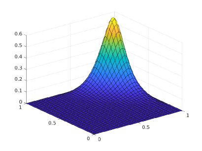
Figure 1. Test case 1. Plot of the exact solution

In Figure 2 we report the behavior of the components of the error estimator $\eta_{h}$ defined as in (51) when the adaptive process is run using $\eta_{h}$ as estimator, based on employing both VEM of order 1 (cf. Figure 2(a)) and of order 2 (cf. Figure 2(b)).

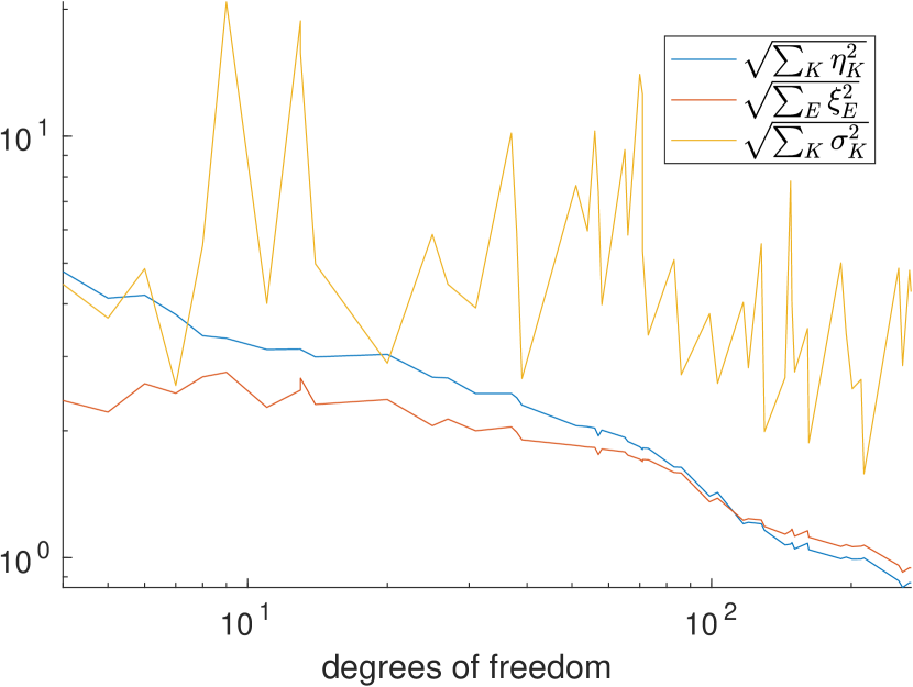
(a) VEM of order 1.

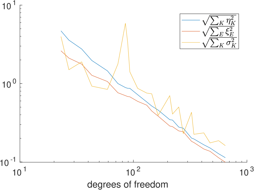
(b) VEM of order 2.

Figure 2. Test case 1. Components of the error estimator $\eta_{h}$ as a function of the number of degrees of freedom, when the adaptive process is driven by the estimator $\eta_{h}$.

From the numerical results reported in Figure 2, we can infer that the three components of the estimator $\eta_{h}$ differ one from each other of an order of magnitude. This behavior is more evident for VEM of order 1, since the larger number of refinements produces large anisotropic elements. A closer inspection, reveals that the factor $M_{K}$ could be much larger than the other factors, and thus the aspect ratio of polygons could largely increase during the anisotropic adaptive process and can drive the adaptive process itself. The large aspect ratio of the elements produced is amplified by the exponent $\frac{5}{4}$ that is present in $M_{K}$ that makes the VEM stabilization dominant with respect to the other components of the estimator (cf. Remark 5.3). The resulting behavior of the estimators might then be not optimal because the large values of $\sigma_{K}$ cause the refinement process to concentrate on cells whose error is already small. Indeed, as we show in Figure 3, the behavior of $\sigma_{K}$ when the refinement process is driven by $\eta_{h}^{\mathrm{heur}}$ tends to be parallel to the one of $\eta_{K}$ and $\xi_{E}$, showing that the behavior of the estimate $\eta_{h}$ is caused by the fact that the estimator $\sigma_{K}$ is selecting for refinement elements that should not be selected. Notice that the above definition of the $\tilde{\sigma}_{K}$ estimator used in $\eta_{h}^{\mathrm{heur}}$ correspond to the one given in Proposition 5.2, setting $M_{K}=1$.

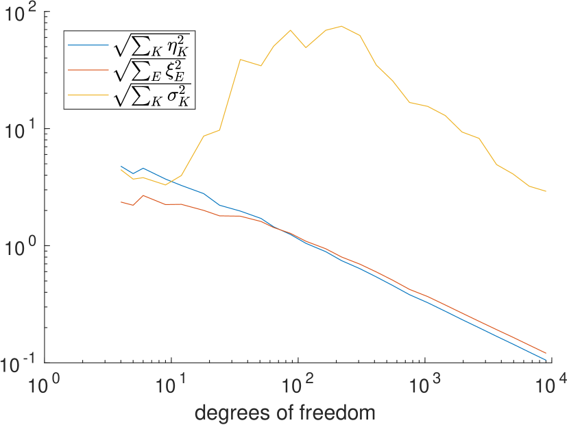
(a) VEM of order 1.

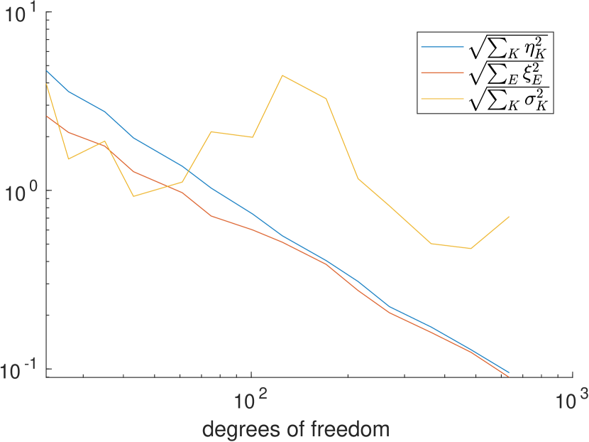
(b) VEM of order 2.

Figure 3. Test case 1. Computed values of $\eta_{K}$, $\xi_{E}$ and $\sigma_{K}$ as a function of the number of degrees of freedom based on employing the heuristically scaled estimator $\eta_{h}^{\mathrm{heur}}$ defined in (55) to drive the adaptive algorithm.

We next analyze the behavior of the error based on employing the heuristically scaled estimator defined in (55) to drive the adaptive algorithm. In Figure 4 we report the color-plot of the solutions and the meshes obtained at the first refinement iteration and at an intermediate adaptive step, based on employing VEM of order 1 and 2, respectively.

(a) VEM of order 1. Adaptive step n. 1.

(b) VEM of order 1. Adaptive step n. 12.

(c) VEM order 2. Adaptive step n. 1.

(d) VEM order 2. Adaptive step n. 7.

Figure 4. Test case 1. Computed solutions and corresponding anisotropic grids at different steps of the adaptive algorithm based on employing the heuristically scaled estimator $\eta_{h}^{\mathrm{heur}}$ defined in (55) to drive the adaptive algorithm.

A zoom of a detail of the computed anisotropic mesh as well as the computed solution at the final adaptive step, are reported in Figure 5, again employing VEM of order 1 and 2.

(a) VEM order 1. Adaptive step n. 25.

(b) VEM order 2. Adaptive step n. 13

Figure 5. Test case 1. Zoom of the computed solutions and corresponding anisotropic grids at the final step of the adaptive algorithm based on employing the heuristically scaled estimator $\eta_{h}^{\mathrm{heur}}$ defined in (55) to drive the adaptive algorithm.

We next compared the behavior of the computed estimator and of the error as a function of the number of the degrees of freedom, again based on employing the heuristically scaled estimator defined in (55) to drive the adaptive algorithm. In Figure 6 we report the computed estimator $\eta_{h}^{\mathrm{heur}}$ and the computed error $\tilde{e}$, plotted against the number of degrees of freedom as well as the convergence rates (computed based on employing a least square fitting). For the sake of comparison, we also report the analogous quantities obtained with the isotropic error estimator $\eta^{\mathrm{iso}}_{h}$ defined in (54), and denoted by $\eta^{\mathrm{iso}}_{h}$ and $\tilde{e}^{\mathrm{iso}}$, respectively. We observe, as expected, that the isotropic adaptive process requires a larger number of degrees of freedom to reduce the error below a given tolerance compared with the anisotropic error estimator.

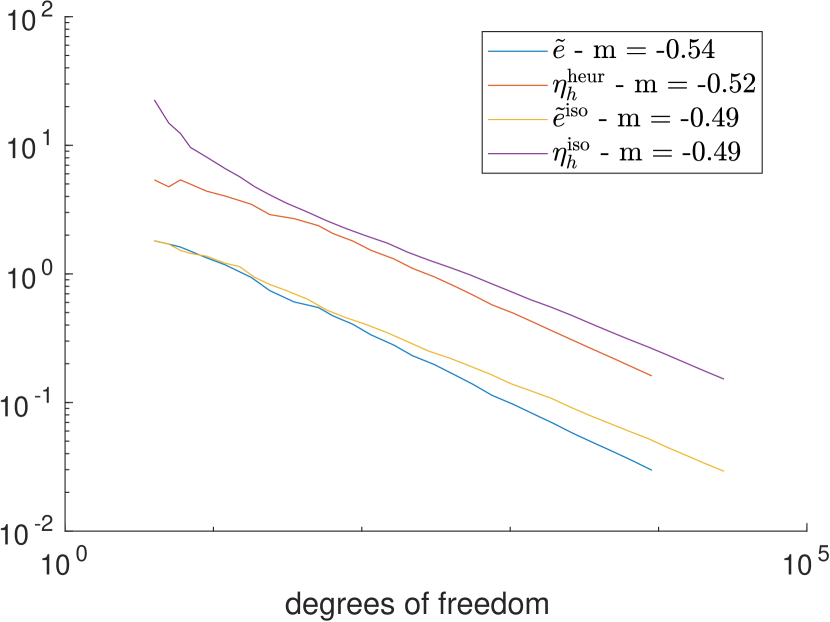
(a) VEM of order 1.

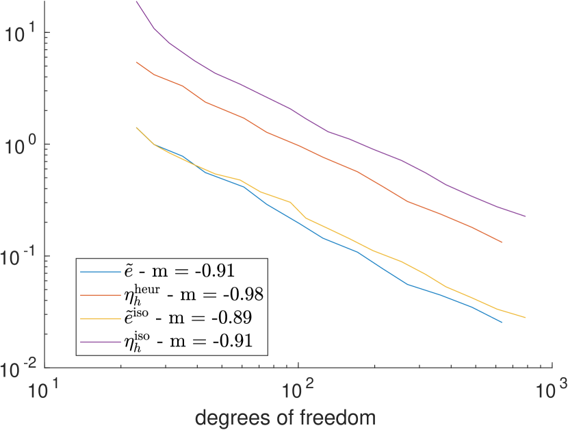
(b) VEM of order 2

Figure 6. Test case 1. Computed values of the estimator $\eta_{h}^{\mathrm{heur}}$, computed errors $\widetilde{e}$ based on employing the exact solution, and corresponding computed convergence rates m as a function of the number of degrees of freedom. The results are compared with the analogous quantities obtained based on employing the isotropic error estimator $\eta^{\mathrm{iso}}_{h}$ defined in (54).

6.3. Test case 2

We have repeated the same set of experiments of the previous section, now choosing the forcing term in such a way that the exact solution is given by

$$u(x,y)=10^{-2}xy(1-x)(1-y)(\mathrm{e}^{10x}-1).$$

We notice that the exact solution of the proposed test case exhibits a steep boundary layer in the $x$-direction close to the right boundary of the domain (see Figure 7).

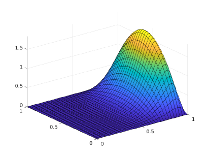
Figure 7. Test case 2. Plot of the exact solution

Next, we report the color-plot of the computed solutions and the corresponding meshes at the initial step of the adaptive algorithm, and after 16 (resp. 9), iterations based on employing VEM of order 1 (resp. 2), and using the heuristically scaled estimator $\eta_{h}^{\mathrm{heur}}$ defined in (55) to drive the adaptive process; cf. Figure 8.

(a) VEM of order 1. Adaptive step n. 1.

(b) VEM of order 1. Adaptive step n. 16.

(c) VEM order 2. Adaptive step n. 1.

(d) VEM order 2. Adaptive step n. 9.

Figure 8. Test case 2. Computed solutions and corresponding anisotropic grids at different steps of the adaptive algorithm based on employing the heuristically scaled estimator $\eta_{h}^{\mathrm{heur}}$ defined in (55) to drive the adaptive algorithm.

A zoom of a detail of the computed anisotropic mesh as well as the corresponding computed solution at the final step of the adaptive algorithm are reported in Figure 9, again employing VEM of order 1 (Figure 9, top) and VEM of order 2 (Figure 9, bottom).

(a) VEM order 1. Adaptive step n. 21.

(b) VEM order 2. Adaptive step n. 13

Figure 9. Test case 2. Zoom of the computed solutions and corresponding anisotropic grids at the final step of the adaptive algorithm based on employing the heuristically scaled estimator $\eta_{h}^{\mathrm{heur}}$ defined in (55) to drive the adaptive algorithm.

Finally, we compare the behavior of the computed estimator and of the error as a function of the number of the degrees of freedom. In Figure 10 we report the estimator $\eta_{h}^{\mathrm{heur}}$ and the error $\tilde{e}$, plotted against the number of degrees of freedom as well as the computed convergence rates. As before, we compare these results with the analogous quantities obtained with the isotropic error estimator $\eta^{\mathrm{iso}}_{h}$ defined in (54). These results have been obtained with VEM of order 1, cf. Figure 10(a) and with VEM of order 2, cf. Figure 10(b). We observe, as expected, that the isotropic adaptive process requires a larger number of degrees of freedom to reduce the error below a given tolerance compared with the anisotropic error estimator.

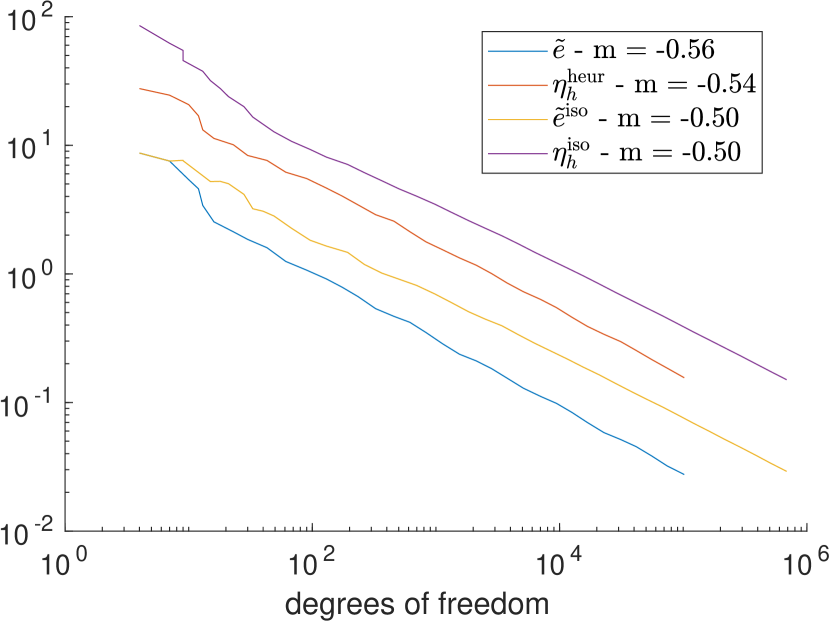
(a) VEM of order 1.

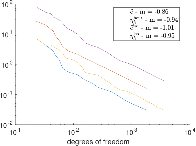
(b) VEM of order 2

Figure 10. Test case 2. Computed values of the estimator $\eta_{h}^{\mathrm{heur}}$, computed errors $\widetilde{e}$ based on employing the exact solution, and corresponding computed convergence rates m as a function of the number of degrees of freedom. The results are compared with the analogous quantities obtained based on employing the isotropic error estimator $\eta^{\mathrm{iso}}_{h}$ defined in (54).

6.4. Test case 3

We have repeated the same set of experiments of the previous section, now choosing the forcing term in such a way that the exact solution is given by

$$u(x,y)=10^{-2}xy(x-1)(y-1)(\mathrm{e}^{10x}-5000x+4499)\,,$$

that is obtained summing an isotropic bubble of the form

$$b(x,y)=50x(1-y)y(0.9-x)(1-x)\,$$

to the solution of the second test case, cf. Figure 11. The manufactured exact solution exhibits a steep boundary layer in the $x$-direction close to the right side of the domain, which requires anisotropic mesh refinement to be efficiently treated and a bubble function in the left part of the domain, which asks for isotropic mesh refinement.

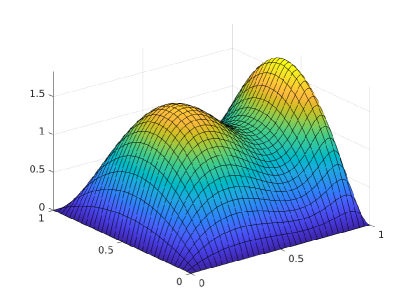
Figure 11. Test case 3. Plot of the exact solution

Next, we report the color-plot of the computed solutions and the meshes obtained at the initial step of the refinement process, and after 17 (resp. 9), iterations based on employing VEM of order 1 (resp. 2), and using the heuristically scaled estimator $\eta_{h}^{\mathrm{heur}}$ defined in (55) to drive the adaptive algorithm; Figure 12 (top) shows the results obtained with VEM of order 1, whereas in Figure 12 (bottom) we show the analogous computations obtained with VEM of order 2.

(a) VEM of order 1. Adaptive step n. 1.

(b) VEM of order 1. Adaptive step n. 17.

(c) VEM order 2. Adaptive step n. 1.

(d) VEM order 2. Adaptive step n. 9.

Figure 12. Test case 3. Computed solutions and corresponding anisotropic grids at different steps of the adaptive algorithm based on employing the heuristically scaled estimator $\eta_{h}^{\mathrm{heur}}$ defined in (55) to drive the adaptive algorithm.

A zoom of a detail of the computed solutions together with the corresponding computed anisotropic meshes at the final step of the adaptive algorithm are reported in Figure 13, again employing VEM of order 1 (left) and VEM of order 2 (right). The reported results show that the combination of isotropic and anisotropic mesh refinement is correctly captured by the adaptive algorithm.

(a) VEM order 1. Adaptive step n. 21.

(b) VEM order 2. Adaptive step n. 18

Figure 13. Test case 3. Zoom of the computed solutions and corresponding anisotropic grids at the final step of the adaptive algorithm based on employing the heuristically scaled estimator $\eta_{h}^{\mathrm{heur}}$ defined in (55) to drive the adaptive algorithm.

Finally, we compare the behavior of the computed estimator and of the error as a function of the number of the degrees of freedom. In Figure 14 we report the estimator $\eta_{h}^{\mathrm{heur}}$ and the error $\tilde{e}$ versus the number of degrees of freedom, together with the computed convergence rates (obtained through a least square fitting). These results have been obtained with VEM of order 1, cf. Figure 14(a) and with VEM of order 2, cf. Figure 14(b). As before, we compare these results with the analogous ones obtained with the isotropic error estimator $\eta^{\mathrm{iso}}_{h}$ defined in (54). Again, as expected, the adaptive algorithm based on employing the anisotropic estimator guarantees a lower error compared with the isotropic one.

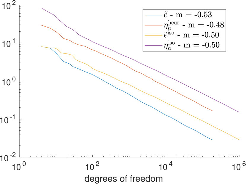
(a) VEM of order 1.

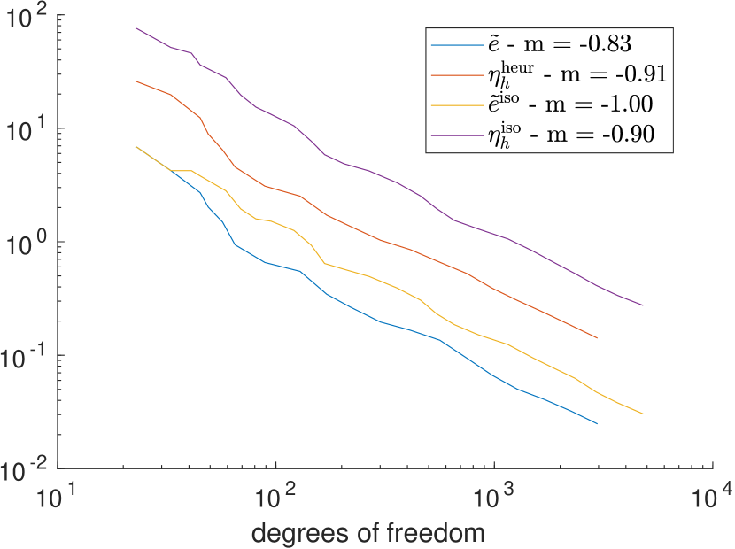
(b) VEM of order 2.

Figure 14. Test case 3. Computed values of the estimator $\eta_{h}^{\mathrm{heur}}$, computed errors $\widetilde{e}$ based on employing the exact solution, and corresponding computed convergence rates m as a function of the number of degrees of freedom. The results are compared with the analogous quantities obtained based on employing the isotropic error estimator $\eta^{\mathrm{iso}}_{h}$ defined in (54).

References

- [1] R. A. Adams and J. J. F. Fournier. Sobolev spaces, volume 140 of Pure and Applied Mathematics (Amsterdam). Elsevier/Academic Press, Amsterdam, second edition, 2003.
- [2] P. F. Antonietti, L. Beirão da Veiga, C. Lovadina, and M. Verani. Hierarchical a posteriori error estimators for the mimetic discretization of elliptic problems. SIAM J. Numer. Anal., 51(1):654–675, 2013.
- [3] P. F. Antonietti, S. Berrone, M. Verani, and S. Weisser. The virtual element method on anisotropic polygonal discretizations. Lecture Notes in Computational Science and Engineering, 126:725–733, 2019.
- [4] T. Apel. Anisotropic finite elements: local estimates and applications. Advances in Numerical Mathematics. B. G. Teubner, Stuttgart, 1999.
- [5] L. Beirão da Veiga. A residual based error estimator for the mimetic finite difference method. Numer. Math., 108(3):387–406, 2008.
- [6] L. Beirão da Veiga and A. Ern. Preface [Special issue—Polyhedral discretization for PDE]. ESAIM Math. Model. Numer. Anal., 50(3):633–634, 2016.
- [7] L. Beirão da Veiga, C. Lovadina, and A. Russo. Stability analysis for the virtual element method. Math. Models Methods Appl. Sci., 27(13):2557–2594, 2017.
- [8] L. Beirão da Veiga and G. Manzini. An a posteriori error estimator for the mimetic finite difference approximation of elliptic problems. Internat. J. Numer. Methods Engrg., 76(11):1696–1723, 2008.
- [9] L. Beirão da Veiga and G. Manzini. Residual a posteriori error estimation for the virtual element method for elliptic problems. ESAIM Math. Model. Numer. Anal., 49(2):577–599, 2015.
- [10] L. Beirão da Veiga, G. Manzini, and L. Mascotto. A posteriori error estimation and adaptivity in virtual elements. Numer. Math., 143(1):139–175, 2019.
- [11] L. Beirão da Veiga, F. Brezzi, A. Cangiani, G. Manzini, L. Marini, and A. Russo. Basic principles of Virtual Element Methods. Mathematical Models and Methods in Applied Sciences, 23(01):199–214, 2013.
- [12] C. Bernardi and V. Girault. A local regularization operator for triangular and quadrilateral finite elements. SIAM J. Numer. Anal., 35(5):1893–1916, 1998.
- [13] S. Berrone and A. Borio. A residual a posteriori error estimate for the Virtual Element Method. Math. Models Methods Appl. Sci., 27(8):1423–1458, 2017.
- [14] S. Berrone, A. Borio, and A. D’Auria. Refinement strategies for polygonal meshes applied to adaptive VEM discretization. arxiv:1912.05403, 2019.
- [15] A. Cangiani, E. H. Georgoulis, T. Pryer, and O. J. Sutton. A posteriori error estimates for the virtual element method. Numer. Math., 137(4):857–893, 2017.
- [16] A. Cangiani and M. Munar. A posteriori error estimates for mixed virtual element methods. arXiv:1904.10054, 2019.
- [17] S. Cao and L. Chen. Anisotropic error estimates of the linear nonconforming virtual element methods. SIAM J. Numer. Anal., 57(3):1058–1081, 2019.
- [18] L. Chen and J. Huang. Some error analysis on virtual element methods. Calcolo, 55(1):Art. 5, 23, 2018.
- [19] H. Chi, L. Beirão da Veiga, and G. H. Paulino. A simple and effective gradient recovery scheme and a posteriori error estimator for the virtual element method (VEM). Comput. Methods Appl. Mech. Engrg., 347:21–58, 2019.
- [20] D. A. Di Pietro and R. Specogna. An a posteriori-driven adaptive mixed high-order method with application to electrostatics. J. Comput. Phys., 326:35–55, 2016.
- [21] L. Formaggia and S. Perotto. New anisotropic a priori error estimates. Numer. Math., 89(4):641–667, 2001.
- [22] L. Formaggia and S. Perotto. Anisotropic error estimates for elliptic problems. Numer. Math., 94(1):67–92, 2003.
- [23] E. H. Georgoulis. Discontinuous Galerkin methods on shape-regular and anisotropic meshes. PhD thesis, Computing Laboratory, University of Oxford, 2003.
- [24] E. H. Georgoulis. –version interior penalty discontinuous Galerkin finite element methods on anisotropic meshes. 3(1):52–79, 2006.
- [25] E. H. Georgoulis, E. Hall, and P. Houston. Discontinuous Galerkin methods for advection-diffusion-reaction problems on anisotropically refined meshes. 30(1):246–271, 2007.
- [26] E. H. Georgoulis, E. Hall, and P. Houston. Discontinuous Galerkin methods on -anisotropic meshes i: a priori error analysis. 1(2-3):221–244, 2007.
- [27] E. H. Georgoulis, E. Hall, and P. Houston. Discontinuous Galerkin methods on -anisotropic meshes. II. A posteriori error analysis and adaptivity. Appl. Numer. Math., 59(9):2179–2194, 2009.
- [28] W. G. Habashi, J. Dompierre, Y. Bourgault, D. Ait-Ali-Yahia, M. Fortin, and M.-G. Vallet. Anisotropic mesh adaptation: towards user-independent, mesh-independent and solver-independent cfd. part i: general principles. International Journal for Numerical Methods in Fluids, 32(6):725–744, 2000.
- [29] D. Mora, G. Rivera, and R. Rodríguez. A posteriori error estimates for a virtual element method for the Steklov eigenvalue problem. Comput. Math. Appl., 74(9):2172–2190, 2017.
- [30] L. Mu. Weak Galerkin based a posteriori error estimates for second order elliptic interface problems on polygonal meshes. J. Comput. Appl. Math., 361:413–425, 2019.
- [31] R. H. Nochetto and A. Veeser. Primer of adaptive finite element methods. In Multiscale and adaptivity: modeling, numerics and applications, volume 2040 of Lecture Notes in Math., pages 125–225. Springer, Heidelberg, 2012.
- [32] R. Verfürth. A posteriori error estimation techniques for finite element methods. Numerical Mathematics and Scientific Computation. Oxford University Press, Oxford, 2013.
- [33] M. Vohralík and S. Yousef. A simple a posteriori estimate on general polytopal meshes with applications to complex porous media flows. Comput. Methods Appl. Mech. Engrg., 331:728–760, 2018.
- [34] S. Weisser. Residual error estimate for BEM-based FEM on polygonal meshes. Numer. Math., 118(4):765–788, 2011.
- [35] S. Weisser. Residual based error estimate and quasi-interpolation on polygonal meshes for high order BEM-based FEM. Comput. Math. Appl., 73(2):187–202, 2017.
- [36] S. Weisser. Anisotropic polygonal and polyedral discretizations in finite element analysis. ESAIM: Mathematical Modelling and Numerical Analysis, 53(2):475–501, 2019.
- [37] S. Weisser. BEM-based Finite Element Approaches on Polytopal Meshes, volume 130 of Lecture Notes in Computational Science and Engineering. Springer International Publishing, 2019.
- [38] S. Weisser and T. Wick. The dual-weighted residual estimator realized on polygonal meshes. Comput. Methods Appl. Math., 18(4):753–776, 2018.
- [39] G. Zenoni, T. Leicht, A. Colombo, and L. Botti. An agglomeration-based adaptive discontinuous Galerkin method for compressible flows. Internat. J. Numer. Methods Fluids, 85(8):465–483, 2017.