Field master equation theory of the self-excited Hawkes process

Abstract

A field theoretical framework is developed for the Hawkes self-excited point process with arbitrary memory kernels by embedding the original non-Markovian one-dimensional dynamics onto a Markovian infinite-dimensional one. The corresponding Langevin dynamics of the field variables is given by stochastic partial differential equations that are Markovian. This is in contrast to the Hawkes process, which is non-Markovian (in general) by construction as a result of its (long) memory kernel. We derive the exact solutions of the Lagrange-Charpit equations for the hyperbolic master equations in the Laplace representation in the steady state, close to the critical point of the Hawkes process. The critical condition of the original Hawkes process is found to correspond to a transcritical bifurcation in the Lagrange-Charpit equations. We predict a power law scaling of the PDF of the intensities in an intermediate asymptotics regime, which crosses over to an asymptotic exponential function beyond a characteristic intensity that diverges as the critical condition is approached. We also discuss the formal relationship between quantum field theories and our formulation. Our field theoretical framework provides a way to tackle complex generalisation of the Hawkes process, such as nonlinear Hawkes processes previously proposed to describe the multifractal properties of earthquake seismicity and of financial volatility.

I Introduction

The self-excited conditional Poisson process introduced by Hawkes Hawkes1 ; Hawkes2 ; Hawkes3 has progressively been adopted as a useful first-order model of intermittent processes with time (and space) clustering, such as those occurring in seismicity and financial markets. The Hawkes process was first used and extended in statistical seismology and remains probably the most successful parsimonious description of earthquake statistics KK1981 ; KK1987 ; Ogata1988 ; Ogata1999 ; HelmsSor02 ; Shyametal2019 . More recently, the Hawkes model has known a burst of interest in finance (see e.g. HawkesRev18 for a short review) as it was realised that some of the stochastic processes in financial markets can be well represented by this class of models FiliSor12 , for which the triggering and branching processes capture the herding nature of market participants (be they due to psychological or rational imitation of human traders or as a result of machine learning and adapting). In field of financial economics, the Hawkes process has been successfully involved in issues as diverse as estimating the volatility at the level of transaction data, estimating the market stability FiliSor12 ; FiliSor15 ; WheatleyWeh2019 , accounting for systemic risk contagion, devising optimal execution strategies or capturing the dynamics of the full order book Bacry1 . Another domain of intense use of the Hawkes model and its many variations is found in the field of social dynamics on the Internet, including instant messaging and blogging such on Twitter Zhao2015 as well as the dynamics of book sales SorDeschatres04 , video views CraneSor08 , success of movies EscobarSor08 , and so on.

The present article, together with the joint-submission Letter KKDS_PRL , can be considered as a sequel complementing a series of papers devoted to the analysis of various statistical properties of the Hawkes process SaiSor2004 ; SaiHSor2005 ; SaiSor2006 ; SaiSorTimes2007 ; SaiSor2014 . These papers have extended the general theory of point processes DalayVere03 to obtain general results on the distributions of total number of events, total number of generations, and so on, in the limit of large time windows. Here, we consider the opposite limit of very small time windows, and characterise the distribution of “intensities”, where the intensity $\nu(t)$ of the Hawkes process at time $t$ is defined as the probability per unit time that an event occurs (more precisely, $\nu(t)dt$ is the probability that an event occurs between $t$ and $t+dt$). We propose a novel natural formulation of the Hawkes process in the form of a field theory of probability density functionals taking the form of a field master equation. This formulation is found to be ideally suited to investigate the hitherto ignored properties of the distribution Hawkes intensities, which we analyse in depth in a series of increasingly sophisticated forms of the memory kernel characterising how past events influence the triggering of future events.

This paper is organised as follows. Section II presents the Hawkes process in its original definition. In addition, we provide a comprehensive review of the previous literature on non-Markovian stochastic processes of diffusive transport developed in traditional statistical physics. Historically, the analytical properties of the generalized Langevin equation (GLE) have been intensively studied and we provide a brief review on the similarity and dissimilarity between the GLE and the Hawkes process from the view point of the Markov embedding of the original non-Markovian one-dimensional dynamics onto a Markovian field dynamics. We then proceed to develop a stochastic Markovian partial differential equation equivalent to the Hawkes process in section III. This is done first for the case where the memory kernel is a single exponential, then made of two exponentials, an arbitrary finite number of exponentials and finally for general memory kernels. It is in section III that the general field master equations are derived. Section IV presents the analytical treatment and provides the solutions of the master equations, leading to the derivation of the probability density function of the Hawkes intensities for the various above mentioned forms of the memory kernel. We also discuss a formal relationship between quantum field theories and our formulation in Section V. Section VI summarises and concludes by outlining future possible extensions of the formalism. These sections are complemented by seven appendices, in which the detailed analytical derivations are provided.

II Model and literature review

II.1 Notation

Firstly, we explain our mathematical notation for stochastic processes. By convention, we denote stochastic variables with a hat symbol, such as $\hat{A}$, to distinguish them from the non-stochastic real numbers $A$, corresponding for instance to a specific realisation of the random variable. The ensemble average of any stochastic variable $\hat{A}$ is also denoted by $\langle\hat{A}\rangle$. The probability density function (PDF) of any stochastic $\hat{A}$ is denoted by $P_{t}(\hat{A}(t)=A)=P_{t}(A)$. The PDF characterizes the probability that $\hat{A}(t)\in[A,A+dA)$ as $P_{t}(A)dA$. Using the notation of the PDF, the ensemble average reads $\langle\hat{A}(t)\rangle:=\int AP_{t}(A)dA$.

We also make the following remark on notations used for our functional analysis. For any function $z(x)\in\mathcal{S}_{F}$ defined for $x\in\bm{R}_{+}=(0,\infty)$ with a function space $\mathcal{S}_{F}$, we can consider a functional $f[\{z(x)\}_{x\in\bm{R}_{+}}]$: i.e., $f:\mathcal{S}_{F}\to\bm{R}$. Functionals in this paper are often abbreviated as $f[z]:=f[\{z(x)\}_{x}]$, with the square brackets emphasized to distinguish from ordinary functions.

II.2 Definition of the Hawkes conditional Poisson process

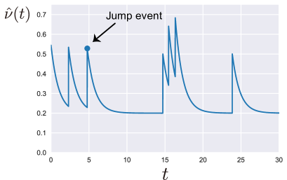
Figure 1: Schematic representation of the Hawkes process (1) with an exponential kernel (13). The event occurring at a given time stamp is represented by a jump in the intensity $\hat{\nu}(t)$, the probability per unit time that a next event will occur.

The Hawkes process is the simplest self-excited point process, which describes with a linear intensity function $\hat{\nu}$ how past events influence the triggering of future events. Its structure is particularly well-suited to address the general and important question occurring in many complex systems of disentangling the exogenous from the endogenous sources of observed activity. It has been and continues to be a very useful model in geophysical, social and financial systems.

The Hawkes process, as any other point process, deals with events (“points” along the time axis). The theory of point processes indeed considers events as being characterised by a time of occurrence but vanishing duration (the duration of events is very small compared to the inter-event times). Thus, to a given event $i$ is associated a time $t_{i}$ of occurrence. In the case where one deals with spatial point processes, the event has also a position ${\vec{r}}_{i}$. And a “mark” $m_{i}$ can be included to describe the event’s size, or its “fertility”, i.e. the average number of events it can trigger directly.

The stochastic dynamics of the Hawkes process is defined as follows. Let us introduce a state variable $\hat{\nu}$, called the intensity. The intensity $\hat{\nu}$ is a statistical measure of the frequency of events per unit time (i.e., a shock occurs during $[t,t+dt)$ with the probability of $\hat{\nu}dt$). In the Hawkes process, the intensity satisfies the following stochastic sum equation (see Fig. 1):

$$\hat{\nu}(t)=\nu_{0}+n\sum_{i=1}^{\hat{N}(t)}h(t-\hat{t}_{i}),$$ (1)

where $\nu_{0}$ is the background intensity, $\{\hat{t}_{i}\}_{i}$ represent the time series of events, $n$ is a positive number called the branching ratio, $h(t)$ is a normalized positive function (i.e., $\int_{0}^{\infty}h(t)dt=1$), and $\hat{N}(t)$ is the number of events during the interval $[0,t)$ (called “counting process”). One often refers to $\hat{\nu}(t)$ as a conditional intensity in the sense that, conditional on the realised sequence of $\hat{N}(t)=k$ (with $k\geq 0$) events, the probability that the $(k+1)$th event occurs during $[t,t+dt)$, such that $\hat{t}_{k+1}\in[t,t+dt)$, is given by $\hat{\nu}(t)dt$. The pulse (or memory) kernel $h(t)$ represents the non-Markovian influence of a given event, and is non-negative definite.

The branching ratio $n$ is a very fundamental quantity, which is the average number of events of first generation (“daughters”) triggered by a given event DalayVere03 ; HelmsSor02 . This definition results from the fact that the Hawkes model, as a consequence of the linear structure of its intensity (1), can be mapped exactly onto a branching process, making unambiguous the concept of generations: more precisely, a given realisation of the Hawkes process can be represented by the set of all possible tree combinations, each of them weighted by a certain probability derived from the intensity function ZhuangVere02 . The branching ratio is the control parameter separating three different regimes: (i) $n<1$: subcritical; (ii) $n=1$: critical and (iii) $n>1$: super-critical or explosive (with a finite probability). The branching ratio $n$ can be shown to be also the fraction of events that are endogenous, i.e., that have been triggered by previous events HelmsSor03 .

II.3 Review of non-Markovian stochastic processes in the framework of the generalized Langevin equation

This subsection provides the background of previous methods for non-Markovian stochastic processes in statistical physics, by focusing on the diffusive dynamics of Brownian particles (e.g., see Refs.Hanggi1990 for detailed reviews). While this class of physical stochastic processes exhibits dynamical characteristics that are quite different from those of the Hawkes processes, our framework can been formally related to such standard theories (in particular for the Markov embedding techniques for non-Markovian processes). We thus offer a comprehensive review to prepare the reader to better understand our theoretical developments. This subsection is written in a self-contained way and is not needed to understand our main results; readers only interested in our formulation can skip this section.

II.3.1 Markovian Langevin equations

Langevin equation.

In the context of statistical physics, non-Markovian stochastic processes have been studied from the viewpoint of diffusion processes KuboB ; ZwanzigB . One of the typical diffusive models is the Langevin equation,

$$M\frac{d\hat{v}(t)}{dt}=-\frac{dU(\hat{x})}{d\hat{x}}-\gamma\hat{v}(t)+\hat{\eta}(t),\>\>\>\frac{d\hat{x}(t)}{dt}=\hat{v}(t),$$ (2)

where $\hat{v}(t)$ and $\hat{x}(t)$ are the velocity and the position of the Brownian particle, $M$ is its mass, $U(\hat{x})$ is the confining potential, $\gamma$ is the viscous friction coefficient, and $\hat{\eta}(t)$ represents the thermal fluctuation modelled by the zero-mean white Gaussian noise. Equation (2) is one of the stochastic differential equations (SDE) first written down in the history of Physics.

The noise term embodying the presence of thermal fluctuation satisfies the fluctuation-dissipation relation (FDR)

$$\langle\hat{\eta}(t)\hat{\eta}(t^{\prime})\rangle=2\gamma T\delta(t-t^{\prime})$$ (3)

where $T$ is the temperature. In this paper, the Boltzmann constant is taken unity: $k_{B}=1$. The FDR must hold for relaxation dynamics near equilibrium states because both viscous friction and thermal fluctuation come from the same thermal environment ZwanzigB .

The standard analytical solution to this Langevin equation can be obtained via the time-evolution equation for the joint PDF $P_{t}(v,x)$, which is given by the Fokker-Planck (FP) equation GardinerB ; VanKampenB :

$$\frac{\partial P_{t}(v,x)}{\partial t}=\mathcal{L}_{\mathrm{FP}}P_{t}(v,x),\>\>\>\mathcal{L}_{\mathrm{FP}}:=-\frac{\partial}{\partial x}v+\frac{\gamma}{M}\left[\frac{\partial}{\partial v}\left(v+\frac{dU(x)}{dx}\right)+\frac{T}{M}\frac{\partial}{\partial v}\right].$$ (4)

It is remarkable that the FP equation is always linear in terms of the PDF even if the Langevin equation has nonlinear terms in general. While there is a one-to-one correspondence between the Langevin equation and the FP equation, the FP equation is often analyzed because the standard methods based on linear algebra is available, such as the eigenfunction expansion.

The Langevin equation (2) can be interpreted as the equation of motion for a Brownian particle, obtained after integrating out the many degrees of freedom of the original microscopic dynamics except for those of the Brownian particles. For example, Eq. (2) can be systematically derived from the Hamiltonian dynamics of the Brownian particle surrounded by a dilute gas (see the kinetic framworks McDonald ; Spohn1980 ; VanKampenB for examples).

Non-Markovian nature as a result of variable elimination.

Let us focus on the case of a harmonic potential $U(\hat{x})={1\over 2}k\hat{x}^{2}$ and eliminate the velocity ZwanzigB , to change the system descriptions from $(\hat{v},\hat{x})$ to $\hat{x}$. By integrating out the velocity degree, we obtain the non-Markovian dynamics for the position $\hat{x}(t)$:

$$\frac{d\hat{x}(t)}{dt}=-\int_{0}^{\infty}dsK(s)\hat{x}(t-s)+\hat{\zeta}(t),\>\>\>\hat{\zeta}(t):=\frac{1}{M}\int_{0}^{\infty}dse^{-\gamma s/M}\hat{\eta}(t-s).$$ (5)

Here, the memory kernel $K(t):=ke^{-\gamma t/M}/M$ represents the retarded potential effect and the noise term $\hat{\zeta}(t)$ is the colored Gaussian noise with zero mean $\langle\hat{\zeta}(t)\rangle=0$ and auto-correlation $\langle\hat{\zeta}(t)\hat{\zeta}(t^{\prime})\rangle=(T/M)e^{-\gamma|t-t^{\prime}|/M}$. Remarkably, the non-Markovian nature has appeared as a result of variable elimination. Here the non-Markovian version of the FDR holds $\langle\hat{\zeta}(t)\hat{\zeta}(t^{\prime})\rangle=\langle x^{2}\rangle_{\rm{eq}}K(|t-t^{\prime}|)$ with equilibrium average $\langle x^{2}\rangle_{\rm{eq}}:=k_{B}T/k$.

II.3.2 Generalized non-Markovian Langevin equation.

While the Markovian Langevin description (2) is reasonable for dilute thermal environments LiReview2013 ; LiNature2010 , such a Markovian description is not available for dense thermal environments, such as liquids LiReview2013 ; Huang2011 ; Franosch2011 . Indeed, Eq. (2) is not valid even for a Brownian particle in water, which is one of the most historically important cases. For such cases, the Langevin description must be modified to accommodate non-Markovian effects originating from hydrodynamic interactions in liquids. The minimal model for such systems is given by the generalized Langevin equation (GLE) KuboB ; ZwanzigB :

$$M\frac{d\hat{v}(t)}{dt}=-\frac{dU(\hat{x})}{d\hat{x}}-\int_{0}^{\infty}dsK(s)\hat{v}(t-s)+\hat{\eta}(t),$$ (6)

where $K(t)$ is the memory kernel for viscous friction and $\hat{\eta}(t)$ is the thermal fluctuation modeled by a colored Gaussian noise with zero mean $\langle\hat{\eta}(t)\rangle=0$. Since both viscous friction and thermal fluctuation share the same origin, they are related to each other via the FDR for non-Markovian processes:

$$\langle\hat{\eta}(t)\hat{\eta}(t^{\prime})\rangle=TK(|t-t^{\prime}|).$$ (7)

For typical three-dimensional liquid systems, the memory kernel has a long tail due to the hydrodynamic retardation effect, such that $K(t)\propto t^{-3/2}$, which was verified by direct experiments in Refs. LiReview2013 ; Huang2011 ; Franosch2011 .

The GLE (6) can be derived from microscopic dynamics by rearrangement of the Liouville operator by the method of the projection operators Mori1965 ; ZwanzigB . Assuming that the initial state of the system is sufficiently close to equilibrium and that a sufficient number of macroscopic variables are accessible via experiments, the projection operator formalism provides a microscopic foundation of the non-Markovian stochastic processes with intuitive physical interpretation.

The solution of the GLE (6) is much harder to obtain than that of the Markovian Langevin equations due to its non-Markovian nature. However, due to the linearity of the dynamics and the Gaussianity of the thermal fluctuations (while they are specific to the GLE equation (6)), all the moments and correlation functions can be analytically calculated based on the Laplace transformation of the SDE Morgado2002 and response functions can be expanded as sums of exponentials through the residue theorems Bao2006 . In addition, the recurrence methods of Ref. Lee1982 are also available for this model.

II.3.3 Origin of the non-Markovian property and Markov embedding

We have seen that the non-Markovian property appears as the result of variable elimination through the example of Eq. (5). This shows that some non-Markovian systems with an exponential memory kernel can be converted back to a Markovian system by adding an auxiliary variable ZwanzigB . This procedure is called Markov embedding Goychuk2009 ; Kupferman2004 and can be generalized to transform the GLE (6) into simultaneous Markovian SDEs when the kernel is given by a sum of exponentials:

$$K(t)=\sum_{k=1}^{K}\kappa_{i}e^{-t/\tau_{i}}\>\>\>\Longrightarrow\>\>\>M\frac{d\hat{v}(t)}{dt}=\sum_{k=1}^{K}\hat{u}_{k}(t),\>\>\>\frac{d\hat{u}_{k}(t)}{dt}=-\frac{\hat{u}_{k}(t)}{\tau_{k}}-\kappa_{k}\hat{v}(t)+\sqrt{\frac{2\kappa_{k}T}{\tau_{k}}}\hat{\xi}^{\mathrm{G}}_{k}(t)$$ (8)

with independent standard Gaussian noises $\hat{\xi}^{\mathrm{G}}_{k}(t)$, satisfying $\langle\hat{\xi}^{\mathrm{G}}(t)_{k}\rangle=0$ and $\langle\hat{\xi}^{\mathrm{G}}_{k}(t)\hat{\xi}^{\mathrm{G}}_{j}(t^{\prime})\rangle=\delta_{kj}\delta(t-t^{\prime})$. Here we have taken the free potential case $U(\hat{x})=0$ for simplicity. We thus find that the exponential-sum memory case is Markovian by introducing the new system-variable set $\hat{\Gamma}:=(\hat{v},\hat{u}_{1},\dots,\hat{u}_{K})$, while it was non-Markovian in the original variable representation $\hat{v}(t)$.

In this sense, whether a system is regarded as Markovian or non-Markovian crucially depends on which variable set is taken for the description of the system. This story is actually consistent with the projection operator formalism: while the original Hamiltonian dynamics obeys the Markovian dynamics (i.e., the time-evolution of the phase-space distribution is given by the Liouville equation), the reduced dynamics of macroscopic variables obeys the non-Markovian Langevin dynamics due to integrating out irrelevant variables. Furthermore, a systematic method of Markov embedding Marchesoni1983 was proposed on the basis of the continued-fraction expansion Mori1965 .

II.3.4 Fokker-Planck descriptions of non-Markovian processes

Compared with Markovian stochastic processes, there are few mathematical techniques that can be applied to the Fokker-Plank (master) equations associated with general non-Markovian processes. One of the formal methods is to use the time-convolution Fokker-Planck equation for macroscopic variables $\bm{x}$: $\partial P_{t}(\bm{x})/\partial t=\int_{0}^{t}ds\mathcal{L}_{\mathrm{GFP}}(\bm{x},s)P_{t-s}(\bm{x})$, which was derived from the projection operator formalism ZwanzigB . Also, some specific class of non-Markovian SDEs can be formulated as a Fokker-Planck equation with time-dependent coefficients via the functional stochastic calculus HanggiReview1995 . While these equations are formally correct, they are not easy to exploit for practical calculations due to their genuine non-Markovian nature.

One of the most powerful approaches to tackle GLE is to use Markov embedding, thus making the system Markovian. This research direction was proposed by Ref. Marchesoni1983 and there are a variety of ways to select the auxiliary variables. By taking the selection in Eq. (8) according to Ref. Goychuk2009 , we obtain the complete Fokker-Planck equation for the GLE with the exponential-sum memory $K(t)=\sum_{k=1}^{K}\kappa_{i}e^{-t/\tau_{k}}$ in the absence of potential $U(\hat{x})=0$,

$$\frac{\partial P_{t}(\Gamma)}{\partial t}=\sum_{k=1}^{K}\left[-\frac{\partial}{\partial v}\frac{u_{k}}{M}+\frac{\partial}{\partial u_{k}}\left(\frac{u_{k}}{\tau_{k}}+\kappa_{k}v\right)+\frac{\kappa_{k}T}{\tau_{k}}\frac{\partial^{2}}{\partial u_{k}^{2}}\right]P_{t}(\Gamma)$$ (9)

for the extended phase point $\Gamma:=(v,u_{1},\dots,u_{K})$ and the corresponding PDF $P_{t}(\Gamma)$.

II.3.5 Field description for an infinite number of auxiliary variables

There are two classes for Markov embedding: one requires a finite number of auxiliary variables (e.g., the GLE with a finite discrete sum of exponential terms to describe the memory (8)), and the other one requires an infinite number of auxiliary variables. The latter class is essentially similar to the classical field theory of stochastic processes, represented by stochastic partial differential equations (SPDE). Indeed, the continuous version of the Markov embedding (8) can be expressed in terms of SPDEs as follows. For the continuous decomposition

$$K(t)=\int_{0}^{\infty}dx\kappa(x)e^{-t/x},$$ (10)

we obtain an equivalent Markov embedding representation in the absence of the potential $U(\hat{x})=0$,

$$\frac{d\hat{v}(t)}{dt}=\frac{1}{M}\int_{0}^{\infty}dxu(t,x),\>\>\>\frac{\partial\hat{u}(t,x)}{\partial t}=-\frac{\hat{u}(t,x)}{x}-\kappa(x)\hat{v}(t)+\sqrt{\frac{2\kappa(x)T}{x}}\hat{\xi}^{\mathrm{G}}(x,t)~{},$$ (11)

with the spatial white Gaussian noise term $\hat{\xi}^{\mathrm{G}}(t,x)$ satisfying $\langle\hat{\xi}^{\mathrm{G}}(t,x)\rangle$=0 and $\langle\hat{\xi}^{\mathrm{G}}(t,x)\hat{\xi}^{\mathrm{G}}(t^{\prime},x^{\prime})\rangle=\delta(x-x^{\prime})\delta(t-t^{\prime})$. This is a simple equation in terms of the time derivative but it can be regarded as a SPDE, since $\hat{u}(t,x)$ is spatially distributed over the auxiliary field $x\in(0,\infty)$. Indeed, this interpretation enables us to apply the functional calculus historically developed for the analytical solution of SPDEs GardinerB .

In the domain of mathematics dealing with SPDEs, the Fokker-Planck description is based on the functional calculus for the field variable (called the functional Fokker-Planck equation in Ref. GardinerB ). The corresponding field Fokker-Planck equation can be derived by replacing the discrete sum with the functional derivative:

$$\frac{\partial P_{t}[\Gamma]}{\partial t}=\int_{0}^{\infty}dx\left[-\frac{\partial}{\partial v}\frac{u(x)}{M}+\frac{\delta}{\delta u(x)}\left(\frac{u(x)}{x}+\kappa(x)v\right)+\frac{\kappa(x)T}{x}\frac{\delta^{2}}{\delta u^{2}(x)}\right]P_{t}[\Gamma]$$ (12)

for the extended phase point $\Gamma:=(v,\{u(x)\}_{x\in(0,\infty)})$ and the corresponding probability functional $P_{t}[\Gamma]$.

We note that the mathematical precise definition of such Fokker-Planck description has not been established yet GardinerB . One can see a formal divergent term in the FP field equation, such as $[\delta/\delta u(x)]u(x)=\delta(0)$. This divergence is irrelevant for physical observables as shown in Sec. V.1.2 since the SPDE is linear. But, general non-linear SPDEs can have divergences even for observables (see the example of the nonlinear stochastic reaction-diffusion model in Ref. GardinerB , Chapter 13.3.3). According to convention, the safest interpretation is that all the procedures are implicitly discrete and the continuous notation is regarded as a useful abbreviation of the discrete underlying model. By introducing the finite lattice constant $dx$ for the auxiliary variable $x$, we have the variable transformations $u_{k}\to u(x_{k})dx$ and $\kappa_{k}\to\kappa(x_{k})dx$. The functional derivative is then introduced as the formal limit of $\delta F[\Gamma]/\delta u(x_{k}):=\lim_{dx\to 0}(\partial F[\Gamma]/\partial u_{k})/dx$ (see Ref. GardinerB , Chapter 13.1.1). In this sense, the derivation of the field Fokker-Planck equation (11) here follows this convention: we first confirm that the discrete Markov embedding (8) works well and then generalize it to its general continuous version (11).

II.3.6 Relation to the non-Markovian Hawkes processes

The above historical discussion of non-Markovian diffusive process provides a clear guideline for different classes of stochastic processes, including the Hawkes process as follows. The summary highlighting dissimilarities and similarities between the GLE and the Hawkes process is presented in Table 1.

Dissimilarities.

The Hawkes process is an example of non-Markovian point processes, triggering finite-size jumps along a sample trajectory. This is in contrast to the non-Markovian Langevin equation, which is based on infinitesimal Gaussian noise to describe the diffusive local transport, and thus does not include trajectory jumps. This difference should be reflected in the form of the time-evolution equation of the PDF. Indeed, the time-evolution of the PDF for the Hawkes process will be shown to obey the master equation (integro-differential equations), while that for the Langevin dynamics obeys the Fokker-Planck equations (second-order derivative equations).

Another dissimilarity comes from the fact that the Hawkes process is an out-of-equilibrium model typically describing a branching process requiring immigrants or background events to drive the whole sequence of events, while the Langevin equations are near-equilibrium models in the sense that initial distributions of the thermal baths are characterized by small perturbations from the Gibbs distribution. Note that the physical validity of the projection operator formalism is not guaranteed in general for out-of-equilibrium systems ZwanzigB characterized by non-Gibbs initial distributions. This conceptual difference is important because the FDR (7) is not necessarily assumed for the Hawkes processes. Indeed, the master equation for the Hawkes process does not satisfy the detailed balance condition GardinerB (or the time-reversal symmetry) as shown later.

We should stress that the word “non-equilibrium” is used here for systems driven by external forces, which leads to non-Gibbs initial distributions for thermal baths in contact with the system. While we did not review these cases in detail, there are various understandings of the FDR. In the historical context of stochastic processes, the FDR is defined as being closely associated with the time-reversal symmetry of the stochastic processes. In this sense, one can mathematically prove that the Hawkes processes is actually “out-of-equilibrium”, in the sense that the corresponding master equation does not satisfy the symmetry condition in Gardiner’s textbook GardinerB . We note that such “out-of-equilibrium” processes are physically reasonable in general non-equilibrium setups. Indeed, the shot noise process GardinerB and the Levy flights dynamics KlafterB can be observed in out-of-equilibrium systems (e.g., see Refs. KanazawaPRL2015 ; KanazawaNature2020 for their statistical-physics derivation from microscopic dynamics), while they do not satisfy the detailed balance condition. In the historical context of the projection operators, the “near-equilibrium condition” is defined such that the initial distribution for the noise-space is characterized by a linear response around the Gibbs distribution. In the context of fluctuation theorems FTJarzynski2000 , the FDR is derived from the assumptions of (1) time-reversal symmetry of the microscopic dynamics and (2) validity of the Gibbs distribution for the thermal bath in contact with the target system. The common understanding is that the noise source (i.e. the thermal bath in contact with the systems) is characterised by a distribution close to the Gibbs distribution. Therefore, there should not be any confusion when considering the Hawkes process for which the FDR is irrelevant.

Similarities.

The GLE (6) can be mapped onto a Markovian process (11) by adding a sufficient number of auxiliary variables. As we show below, the same Markov embedding technique is available even for the non-Markovian Hawkes processes (1), by adding a sufficient number of auxiliary variables. Since the memory kernel can be a continuous sum of exponential kernels, the most general description of the Hawkes process should be based on an infinite number of auxiliary variables. As discussed above, such systems are typically described as a classical field theory driven by stochastic terms and thus the dynamics of the original Hawkes process can be finally mapped onto an SPDE (36) and the field master equations (40).

Model	GLE (exponential memory)	GLE (general memory)	Hawkes process (general memory)
Character	Diffusive transport	Diffusive transport	Point process
Fundamental equation	Fokker-Planck equation (9)	Field Fokker-Planck equation (12)	Field master equation (40)
Typical systems	Near equilibrium	Near equilibrium	Out-of-equilibrium
Phenomena	Relaxation	Relaxation	Critical bursts
FDR	Yes	Yes	No
Non-Markovian representation	SDE (6)	SDE (6)	SDE (1)
Markovian representation	SDE (8)	SPDE (11)	SPDE (36)
# of auxiliary variables	finite	inifinite (field description)	infinite (field description)

Table 1: Summary table to compare the generalized Langevin equation and the Hawkes process. Here FDR stands for the fluctuation-dissipation relation.

III Master equations

We now formulate the master equation for the model (1) and provide its asymptotic solution around the critical point.

III.1 Markov embedding: introduction of auxiliary variables

As discussed in Sec. II.3.3, non-Markovian properties in many stochastic systems often arise as a result of variable eliminations. This suggests that, reciprocally, it might be possible to map a non-Markovian system onto a Markovian one by adding auxiliary variables (i.e., Markov embedding). While the Hawkes process (1) is non-Markovian in its original representation only based on the intensity $\hat{\nu}(t)$, it can be also transformed onto a Markovian process by selecting an appropriate set of system variables. In this section, we formulating such a Markov embedding procedure to derive the corresponding master equations.

III.2 The single exponential kernel case

III.2.1 Mapping to Markovian dynamics

Before developing the general framework for arbitrary memory kernel $h(t)$, we consider the simplest case of an exponential memory kernel:

$$h(t)=\frac{1}{\tau}e^{-t/\tau},$$ (13)

satisfying the normalization $\int_{0}^{\infty}h(t)dt=1$. The decay time $\tau$ quantifies how long an event can typically trigger events in the future. This special case is Markovian as discussed in Refs. Oakes1975 ; Dassios2011 , because the lack of memory of exponential distributions ensures that the number of events after time $t$ defines a Markov process in continuous time Knopoff1997 .

As shown in the example (5), some non-Markovian processes can be mapped onto a Markovian stochastic system if the memory function is exponential. Here we show that, likewise, this single exponential case (13) can be mapped onto an SDE driven by a state-dependent Markovian Poisson noise. By decomposing the intensity as

$$\hat{z}:=\hat{\nu}-\nu_{0},$$ (14)

let us consider the Langevin dynamics

$$\frac{d\hat{z}}{dt}=-\frac{1}{\tau}\hat{z}+\frac{n}{\tau}\hat{\xi}^{\mathrm{P}}_{\hat{\nu}}$$ (15)

with a state-dependent Poisson noise $\hat{\xi}^{\mathrm{P}}_{\hat{\nu}}$ with intensity given by $\hat{\nu}=\hat{z}+\nu_{0}$ and initial condition $\hat{z}(0)=0$. The introduction of $\hat{z}$ is similar to the trick proposed in BouchaudTradebook2018 for an efficient estimation of the maximum likelihood of the Hawkes process. By expressing the state-dependent Poisson noise as

$$\hat{\xi}^{\mathrm{P}}_{\hat{\nu}}(t)=\sum_{i=1}^{\hat{N}(t)}\delta(t-\hat{t}_{i}),$$ (16)

we obtain the formal solution of equation (15)

$$\hat{\nu}(t)=\nu_{0}+\hat{z}(t)=\nu_{0}+\frac{n}{\tau}\int_{0}^{t}dt^{\prime}e^{-(t-t^{\prime})/\tau}\hat{\xi}^{\mathrm{P}}_{\hat{\nu}}(t^{\prime})=\nu_{0}+n\sum_{i=0}^{\hat{N}(t)}h(t-\hat{t}_{i}).$$ (17)

This solution shows that the SDE (15) is equivalent to the Hawkes process (1). Equation (15) together with (16) is therefore a short hand notation for

$$\hat{z}(t+dt)-\hat{z}(t)=\begin{cases}-\frac{1}{\tau}\hat{z}(t)dt&(\mbox{No jump during $[t,t+dt)$; probability}=1-\hat{\nu}(t)dt)\\ \frac{n}{\tau}&(\mbox{Jump in $[t,t+dt)$; probability}=\hat{\nu}(t)dt)\end{cases}$$ (18)

for the probabilistic time evolution during $[t,t+dt)$ (see Fig. 2a for a schematic representation). Note that the event probability explicitly depends on $\hat{\nu}(t)$, which reflects the endogenous nature of the Hawkes process. This is the first example of the Markov embedding of the Hawkes process. Note that this procedure corresponds to Eq. (8) for the case of the GLE with $K=1$.

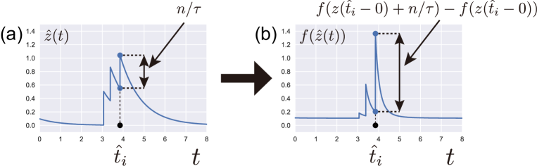
Figure 2: (a) Schematic representation of a typical trajectory for $\hat{z}(t)$ defined by (14). A jump of size $n/\tau$ may occur in the time interval $[t,t+dt)$ with probability $\hat{\nu}(t)dt$. (b) Let us consider an arbitrary function $f(\hat{z})$. At the time $t=\hat{t}_{i}$ of the jump, there is a corresponding jump in the trajectory of $f(\hat{z})$, which is characterized by $df(\hat{z}(t)):=f(\hat{z}(\hat{t}_{i}-0)+n/\tau)-f(\hat{z}(\hat{t}_{i}-0))$. The plots shown here are based on a numerical simulation with the following parameters: $\tau=1$, $n=0.5$, $\nu_{0}=0.1$ and $f(z)=\exp[5(z-1)]+0.1$.

III.2.2 Master equation

By introducing equation (15) together with (16), we have transformed a non-Markovian point process into a Markovian SDE. This allows us to derive the corresponding master equation for the probability density function (PDF) $P_{t}(z)$ of the excess intensity $\hat{z}$ (14),

$$\frac{\partial P_{t}(z)}{\partial t}=\frac{1}{\tau}\frac{\partial}{\partial z}zP_{t}(z)+\Big{[}(\nu_{0}+z-n/\tau)P_{t}(z-n/\tau)-(\nu_{0}+z)P_{t}(z)\Big{]},$$ (19)

with the boundary condition

$$P_{t}(z)\Big{|}_{z=0}=0$$ (20)

$P_{t}(z)dz$ is thus the probability that $\hat{z}(t)$ takes a value in the interval $\hat{z}(t)\in[z,z+dz)$ at time $t$. We note that this master equation after Markov embedding corresponds to the FP equation (9) for the case of the GLE with $K=1$.

The master equation (19) is derived as follows. Let us consider an arbitrary function $f(\hat{z})$. Using (18), its time evolution during $[t,t+dt)$ is given by

$$f(\hat{z}(t+dt))-f(\hat{z}(t))=\begin{cases}-\frac{\hat{z}(t)}{\tau}\frac{\partial f(\hat{z}(t))}{\partial\hat{z}}dt&(\mbox{Probability}=1-\hat{\nu}(t)dt)\\ f(\hat{z}(t)+n/\tau)-f(\hat{z}(t))&(\mbox{Probability}=\hat{\nu}(t)dt)\end{cases},$$ (21)

as schematically illustrated in Fig. 2b. By taking the ensemble average of both sides, we obtain

$$dt\int dz\frac{\partial P_{t}(z)}{\partial t}f(z) =\int dzP_{t}(z)\left[-\frac{z}{\tau}\frac{\partial f(z)}{\partial z}dt+(z+\nu_{0})\{f(z+n/\tau)-f(z)\}dt\right],$$

$$\Longrightarrow\int dz\frac{\partial P_{t}(z)}{\partial t}f(z) =\int dzf(z)\left[\frac{1}{\tau}\frac{\partial}{\partial z}zP_{t}(z)+\{(\nu_{0}+z-n/\tau)P(z-n/\tau)-(\nu_{0}+z)P(z)\}\right].$$ (22)

This result (22) is obtained by (i) using the identity

$$\left<f(\hat{z}(t+dt))-f(\hat{z}(t))\right>=\int dz[P_{t+dt}(z)-P_{t}(z)]f(z)=dt\int dz\frac{\partial P_{t}(z)}{\partial t}f(z),$$ (23)

(ii) by performing a partial integration of the first term in the right-hand side of Eq. (22), and (iii) by introducing the change of variable $z\to z-n/\tau$ for the second term. Since (22) is an identity holding for arbitrary $f(z)$, the integrants of the lelf-hand-side and right-hand-side must be equal for arbitrary $f(z)$, which yields the master equation (19).

Note that the above derivation of the master equation is not restricted to the exponential shape of the memory kernel. We are going to use the same derivation in the more complex examples discussed below. We also note that the master equation (19) does not satisfy the detailed balance condition of Ref. GardinerB , which reflects the fact that the Hawkes process is a model for out-of-equilibrium systems.

III.3 Discrete sum of exponential kernels

III.3.1 Mapping to Markovian dynamics

The above formulation can be readily generalized to the case of a memory kernel expressed as a discrete sum of exponential functions:

$$h(t)=\frac{1}{n}\sum_{k=1}^{K}\frac{n_{k}}{\tau_{k}}e^{-t/\tau_{k}}.$$ (24)

In this case, each coefficient $n_{k}$ quantifies the contribution of the $k$-th exponential with memory length $\tau_{k}$ to the branching ratio $n=\sum_{k=1}^{K}n_{k}$, satisfying the normalization $\int_{0}^{\infty}h(t)dt=1$. We note that this representation (24) is quite general, as it can approximate well the case of a power-law kernel with cut-off up to a constant Hardimanetal2013 .

Harris suggested the intuitive notion that it is possible to map this case to a Markovian dynamics if the state of the system at time $t$ is made to include the list of the ages of all events Harris1963 . The problem is that this conceptual approach is unworkable in practice due to the exorbitant size of the required information. By introducing an auxiliary age pyramid process, Ref. Boumezoued2016 identified some key components to add to the Hawkes process and its intensity to make the dynamics Markovian. Here, in order to map model (1) onto a Markovian stochastic process, we propose a more straightforward Markov embedding approach, which generalised the previous case of a single exponential memory function. We decompose the intensity into a sum of $K$ excess intensities $\{z_{k}\}_{k=1}^{K}$ as follows:

$$\hat{\nu}(t)=\nu_{0}+\sum_{k=1}^{K}\hat{z}_{k}(t)~{}.$$ (25)

Each excess intensity $\hat{z}_{k}$ is the solution of a Langevin equation driven by a state-dependent Markovian Poisson shot noise

$$\frac{d\hat{z}_{k}}{dt}=-\frac{\hat{z}_{k}}{\tau_{k}}+\frac{n_{k}}{\tau_{k}}\hat{\xi}^{\mathrm{P}}_{\hat{\nu}}~{}.$$ (26)

Note that the same state-dependent Poisson noise $\hat{\xi}^{\mathrm{P}}_{\hat{\nu}}(t)$ defined by expression (16) acts on the Langevin equation for each excess intensity $\{\hat{z}_{k}\}_{k=1,\dots,K}$. In other words, each shock event impacts simultaneous the trajectories for all excess intensities $\{\hat{z}_{k}\}_{k=1,\dots,K}$ (see the vertical broken line in Fig. 3a and 3b and the resulting trajectory of $\hat{\nu}(t)$ in Fig. 3c). Note that this Markov embedding corresponds to Eq. (8) for the case of the GLE.

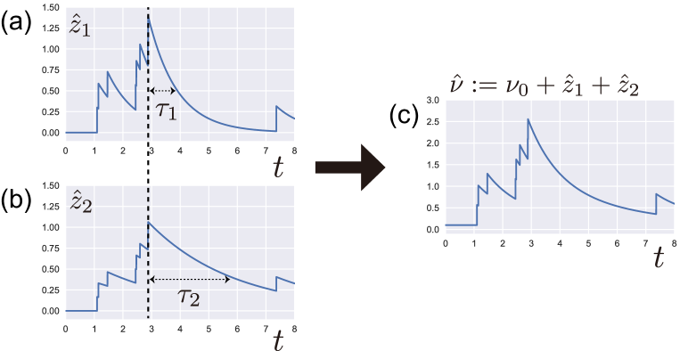
Figure 3: Case where the memory kernel is the sum of two exponentials. Panels (a) and (b) show the schematic trajectories of the two excess intensities $\hat{z}_{1}$ and $\hat{z}_{2}$ and panel (c) that of the resulting total intensity $\hat{\nu}:=\nu 0+\hat{z}_{1}+\hat{z}_{2}$. The parameters are $K=2$, $\tau_{1}=1$, $n_{1}=0.3$, $\tau_{2}=3$, $n_{2}=0.5$ (and thus $n=0.8$) and $\nu_{0}=0.1$.

III.3.2 Master equation

As the set of SDEs for $\hat{\bm{z}}:=(\hat{z}_{1},\hat{z}_{2},\dots,\hat{z}_{K})^{\mathrm{T}}$ are standard Markovian stochastic processes, we obtain the corresponding master equation:

$$\frac{\partial P_{t}(\bm{z})}{\partial t}=\sum_{k=1}^{K}\frac{\partial}{\partial z_{k}}\frac{z_{k}}{\tau_{k}}P_{t}(\bm{z})+\left[\left\{\nu_{0}+\sum_{k=1}^{K}(z_{k}-n_{k}/\tau_{k})\right\}P_{t}(\bm{z}-\bm{h})-\left\{\nu_{0}+\sum_{k=1}^{K}z_{k}\right\}P_{t}(\bm{z})\right].$$ (27)

The jump-size vector is given by $\bm{h}:=(n_{1}/\tau_{1},n_{2}/\tau_{2},\dots,n_{K}/\tau_{K})^{\mathrm{T}}$. The PDF $P_{t}(\bm{z})$ obeys the following boundary condition

$$P_{t}(\bm{z})\Big{|}_{\bm{z}\in\partial\bm{R}^{K}_{+}}=0~{},$$ (28)

on the boundary $\partial\bm{R}^{K}_{+}:=\{\bm{z}|z_{k}=0\mbox{ for some }k\}$. This equation (27) can be derived following the procedure used for the single exponential case that led us to the master equation (19) (see Appenedix A.1 for an explicit derivation). Note that this master equation corresponds to the FP equation (9) for the case of the GLE.

III.3.3 Laplace representation of the master equation

The master equation (27) takes a simplified form under the Laplace representation,

$$\tilde{P}_{t}(\bm{s}):=\mathcal{L}_{K}[P_{t}(\bm{z});\bm{s}]~{},$$ (29)

where the Laplace transformation in the $K$ dimensional space is defined by

$$\mathcal{L}_{K}[f(\bm{z});\bm{s}]:=\int_{0}^{\infty}d\bm{z}e^{-\bm{s}\cdot\bm{z}}f(\bm{z})$$ (30)

with volume element $d\bm{z}:=\prod_{k=1}^{K}dz_{k}$. The wave vector $\bm{s}:=(s_{1},\dots,s_{K})^{\mathrm{T}}$ is the conjugate of the excess intensity vector $\bm{z}:=(z_{1},\dots,z_{K})^{\mathrm{T}}$.

The Laplace representation of the master equation (27) is then given by

$$\frac{\partial\tilde{P}_{t}(\bm{s})}{\partial t}=-\sum_{k=1}^{K}\frac{s_{k}}{\tau_{k}}\frac{\partial\tilde{P}_{t}(\bm{s})}{\partial s_{k}}+\left(e^{-\bm{h}\cdot\bm{s}}-1\right)\left(\nu_{0}-\sum_{k=1}^{K}\frac{\partial}{\partial s_{k}}\right)\tilde{P}_{t}(\bm{s}).$$ (31)

Then, the Laplace representation (29) of $P_{t}(\bm{z})$, which is the solution of (31), allows us to obtain the Laplace representation $\tilde{Q}_{t}(s)$ of the intensity PDF $P_{t}(\nu)$ according to

$$\tilde{Q}_{t}(s):=\mathcal{L}_{1}[P_{t}(\nu);s]=\left<e^{-s(\nu_{0}+\sum_{k=1}^{K}\hat{z}_{k})}\right>=e^{-\nu_{0}s}\tilde{P}_{t}\left(\bm{s}=(s,s,\dots,)^{\mathrm{T}}\right)~{}.$$ (32)

III.4 General kernels

III.4.1 Mapping to Markovian dynamics

The above formulation can be generalized to general forms of the memory kernel. Let us decompose the kernel as a continuous superposition of exponential kernels,

$$h(t)=\frac{1}{n}\int_{0}^{\infty}\frac{n(x)}{x}e^{-t/x}dx~{},\>\>\>n=\int_{0}^{\infty}n(x)dx~{},$$ (33)

where we have introduced the set of continuous auxiliary variables $x\in\bm{R}_{+}$. This decomposition satisfies the normalization condition $\int_{0}^{\infty}h(t)dt=1$. Here we use the notation $x$ for these auxiliary variables to emphasise the formal connection with the usual field theory of classical stochastic (or quantum) systems. Indeed, the observables will be defined over the “field” $x\in\bm{R}_{+}$. The function $n(x)$ quantifies the contribution of the $x$-th exponential with memory length $x$ to the branching ratio. We can then interpret $n(x)/n$ as a normalised distribution of time scales present in the memory kernel of the Hawkes process. As we show below, an important condition for solvability will be the existence of its first-order moment

$$\frac{\alpha}{n}:=\langle\tau\rangle:=\int_{0}^{\infty}x\frac{n(x)}{n}dx<\infty~{}.$$ (34)

This condition (34) means that $n(x)$ should decay faster than $1/x^{2}$ at large $x$’s. Hence, the representation (33) implies that the memory kernel has to decay at large times faster than $1/t^{2}$. This covers situations where the variance of the time scales embedded in the memory kernel diverges. But this excluded the cases $h(t)\sim 1/t^{1+\theta}$ with $0<\theta<1$ that are relevant to the Omori law for earthquakes SorDeschatres04 ; CraneSor08 and to the response to social shocks SaiSor2004 . This case $0<\theta<1$ for which $\alpha$ diverges needs to be treated separately and this is beyond the content of the present work.

We then decompose the intensity of the Hawkes process as a continuous sum of excess intensities $\hat{z}(t,x)$

$$\hat{\nu}(t)=\nu_{0}+\int_{0}^{\infty}dx\hat{z}(t,x)~{}.$$ (35)

Each excess intensities $\hat{z}_{t}(\tau)$ is the solution of the following dynamical equation

$$\frac{\partial\hat{z}(t,x)}{\partial t}=-\frac{\hat{z}(t,x)}{x}+\hat{\eta}(t,x),\>\>\>\hat{\eta}(t,x):=\frac{n(x)}{x}\hat{\xi}^{\mathrm{P}}_{\hat{\nu}},$$ (36)

where, as for the previous case of a discrete sum of exponentials, the same state-dependent Poisson noise $\hat{\xi}^{\mathrm{P}}_{\hat{\nu}}(t)$ defined by expression (16) acts on the Langevin equation for each excess intensity $\hat{z}(t,x)$. While Eq. (36) is a simple equation only related to the time derivative, this equation can be regarded as an SPDE since $\hat{z}(t,x)$ is distributed over the auxiliary variable field $x\in(0,\infty)$. Furthermore, this interpretation allows us to use functional calculus, historically developed for the solution of SPDEs (such as the stochastic reaction-diffusion equations GardinerB ). Note that this SPDE corresponds to Eq. (11) for the case of the GLE.

The set of SPDEs (36) expresses the fact that the continuous field of excess intensity $\{\hat{z}(t,x)\}_{x\in\bm{R}_{+}}$ tends to relax to zero, but they are intermittently simultaneously shocked by the shared shot noise term $\hat{\xi}^{\mathrm{P}}_{\hat{\nu}}$, with a $x$-dependent jump size $n(x)/x$. This is in contrast to the SPDE representation (11) for the GLE (6), where the noise term at $x$ has no correlation with that at another point $x^{\prime}$: $\langle\hat{\xi}^{\mathrm{G}}(t,x)\hat{\xi}^{\mathrm{G}}(t,x^{\prime})\rangle=0$ for $x\neq x^{\prime}$. In a more conventional expression, we can rewrite the long-range nature of the spatial correlation in $\hat{\eta}(t,x)$ as

$$\langle\hat{\eta}(t,x)\hat{\eta}(t,x^{\prime})\rangle_{\mathrm{ss}}=\mathcal{K}(x,x^{\prime})\delta(t-t^{\prime}),\>\>\>\mathcal{K}(x,x^{\prime})=\frac{n(x)n(x^{\prime})}{xx^{\prime}}\langle\hat{\nu}\rangle_{\mathrm{ss}}.$$ (37)

If $K(x,x^{\prime})$ was a $\delta$ function, the SPDE could be regarded as a non-interacting infinite variable systems. This long-range nature means that all the excess intensity $\hat{z}(t,x)$ at different points are strongly correlated through this noise term, even though the SPDE (36) has no spatial derivatives.

III.4.2 Field master equation

The master equation corresponding to the SDE (36) can be derived by following the same procedure presented for the simple exponential case and for the discrete sum of exponentials. There is however a technical difference since the state of the system is now specified by the continuous field variable $\{\hat{z}(t,x)\}_{x\in\bm{R}_{+}}$. Thus, the probability density function is replaced with the probability density functional $P[\{\hat{z}(t,x)=z(x)\}_{x\in\bm{R}_{+}}]=P_{t}[\{z(x)\}_{x\in\bm{R}_{+}}]$. In other words, the probability that the system state is in the state specified by $\{z(x)\}_{x\in\bm{R}_{+}}$ at time $t$ is characterized by $P_{t}[\{z(x)\}_{x\in\bm{R}_{+}}]\mathcal{D}z$ with functional integral volume element $\mathcal{D}z$.

We use the notational convention that any mapping with square bracket $A[\{f(x)\}_{x\in\bm{R}_{+}}]$ indicates that the map $A$ is a functional of $\{f(x)\}_{x\in\bm{R}_{+}}$. In addition, we sometimes abbreviate the functional $P_{t}[\{z(x)\}_{x\in\bm{R}_{+}}]$ by $P_{t}[z]:=P_{t}[\{z(x)\}_{x\in\bm{R}_{+}}]$ for the sake of brevety.

The presence of a continuous field variable leads to several technical issues, such as in the correct application of the Laplace transform. The functional Laplace transformation $\mathcal{L}_{\mathrm{path}}$ of an arbitrary functional $f[z]$ is defined by a functional integration (i.e., a path integral):

$$\mathcal{L}_{\mathrm{path}}\big{[}f[z];s\big{]}:=\int\mathcal{D}ze^{-\int_{0}^{\infty}dxs(x)z(x)}f[z]~{}.$$ (38)

This allows us to define the Laplace representation of the probability density functional by

$$\tilde{P}_{t}[s]:=\mathcal{L}_{\mathrm{path}}\big{[}P_{t}[z];s\big{]}$$ (39)

for an arbitrary nonnegative function $\{s(\tau)\}_{\tau\in\bm{R}_{+}}$.

As the natural extension of Eq. (27), the master equation for the probability density functional is given by

$$\frac{\partial P_{t}[z]}{\partial t}=\int_{0}^{\infty}dx\frac{\delta}{\delta z(x)}\frac{z(x)}{x}P_{t}[z]+\Bigg{[}\left\{\nu_{0}+\int_{0}^{\infty}(z-n/x)dx\right\}P_{t}[z-n/x]-\left\{\nu_{0}+\int_{0}^{\infty}zdx\right\}P_{t}[z]\Bigg{]}$$ (40)

with the boundary condition

$$P_{t}[z]\Big{|}_{z\in\partial\bm{R}^{\infty}_{+}}=0$$ (41)

where the boundary of the function space $\partial\bm{R}^{\infty}_{+}:=\{z|z(x)=0\mbox{ for some }x\in[0,\infty)\}$. This field master equation after Markov embedding corresponds to the FP field equation (11) for the GLE.

Interpretation.

As discussed in Sec. II.3.5, one of the safest interpretations is to regard this functional description as the formal continuous limit from the discrete description in Sec. III.3. By introducing a finite lattice interval $dx>0$ and rewriting $\tau_{k}\to x_{k}$, $\hat{z}_{k}(t)\to\hat{z}(t,x_{k})dx$, and $n_{k}\to n(x_{k})dx$, Eqs. (24) - (26) can be rewritten as

$$h(t)=\frac{1}{n}\sum_{k=1}^{K}\frac{n(x_{k})}{x_{k}}e^{-t/x_{k}}dx,\>\>\>\hat{\nu}(t)=\nu_{0}+\sum_{k=1}^{K}\hat{z}(t,x_{k})dx,\>\>\>\frac{\partial z(t,x_{k})}{\partial t}=-\frac{\hat{z}(t,x_{k})}{x_{k}}+\frac{n(x_{k})}{x_{k}}\hat{\xi}^{\mathrm{P}}_{\hat{\nu}}(t).$$ (42)

The master equation (27) is rewritten as

$$\frac{\partial P_{t}(\bm{z})}{\partial t}=\sum_{k=1}^{K}dx\left[\frac{1}{dx}\frac{\partial}{\partial z(x_{k})}\right]\frac{z(x_{k})}{x_{k}}P_{t}(\bm{z})+\left\{\nu_{0}+\sum_{k=1}^{K}(z(x_{k})-n(x_{k})/x_{k})dx\right\}P_{t}(\bm{z}-\bm{h})-\left\{\nu_{0}+\sum_{k=1}^{K}z(x_{k})dx\right\}P_{t}(\bm{z}).$$ (43)

According to the convention in Ref. GardinerB , we take a formal limit $K\to\infty$ and $dx\to 0$ to apply the formal replacement

$$\int_{0}^{\infty}dx[...]:=\lim_{dx\to 0}\sum_{k=1}^{K}dx[...],\>\>\>\frac{\delta}{\delta z(x)}:=\lim_{dx\to 0}\frac{1}{dx}\frac{\partial}{\partial z(x_{k})}.$$ (44)

The master equation (40) for the field variables $\{\hat{z}(t,x)\}_{x\in(0,\infty)}$ is thus derived. While this derivation is based on a formal limit of a discrete description, Eq. (40) can be also derived by direct continuous operations based on the functional Taylor expansions (See Appendix. A.2 for the detailed derivation based on functional calculus).

We remark that the SPDE (36) is linear and serious divergence problems did not appear at least for our main results on physical observables. In addition, our final results have been confirmed to be robust for both discrete and continuous cases as shown later. This strategy is consistent with the safe prescription suggested in Ref. GardinerB : in the beginning, the functional descriptions for field variables should be based on a discrete formulation. The continuous description should be introduced afterward as a formal limit of zero-lattice intervals. In this sense, our analysis has successfully avoided the delicate divergence problems on general SPDEs.

III.4.3 Laplace representation of the master equation

In the functional Laplace representation (39), the master equation (40) takes the following simple first-order functional differential equation

$$\frac{\partial\tilde{P}_{t}[s]}{\partial t}=\nu_{0}\left(e^{-\int_{0}^{\infty}dx^{\prime}s(x^{\prime})n(x^{\prime})/x^{\prime}}-1\right)\tilde{P}_{t}[s]-\int_{0}^{\infty}dx\left(e^{-\int_{0}^{\infty}dx^{\prime}s(x^{\prime})n(x^{\prime})/x^{\prime}}-1+\frac{s(x)}{x}\right)\frac{\delta\tilde{P}_{t}[s]}{\delta s(x)}~{}.$$ (45)

III.4.4 General formulation

All the above forms of the memory kernel can be unified by remarking that the variable transformation (33) is equivalent to a Laplace transform, since it can be rewritten as

$$h(t)=\frac{1}{n}\int_{0}^{\infty}\frac{1}{s}n\left(\frac{1}{s}\right)e^{-st}ds=\frac{1}{n}\mathcal{L}_{1}\left[\frac{1}{s}n\left(\frac{1}{s}\right);t\right]\>\>\>\>\Longleftrightarrow\>\>\>\>\frac{n(x)}{n}=\frac{1}{x}\mathcal{L}^{-1}_{1}\left[h(t);s\right]\bigg{|}_{s=1/x}.$$ (46)

This allows us to reformulate the several examples discussed above in a unified way presented in Table 2.

Case	$\displaystyle h(t)$	$\displaystyle n(x)$
Single exponential kernel	$\displaystyle\frac{1}{\tau_{1}}e^{-t/\tau_{1}}$	$\displaystyle n_{1}\delta(x-\tau_{1})$
Discrete superposition of exponential kernel	$\displaystyle\frac{1}{n}\sum_{k=1}^{K}\frac{n_{k}}{\tau_{k}}e^{-t/\tau_{k}}$	$\displaystyle\sum_{k=1}^{K}n_{k}\delta(x-\tau_{k})$
Power-law kernel $(\beta\geq 0)$	$\displaystyle\frac{1}{\tau^{*}}\frac{\beta}{(1+t/\tau^{*})^{\beta+1}}$	$\displaystyle\frac{n}{x}\left(\frac{\tau^{*}}{x}\right)^{\beta}\frac{e^{-\tau^{*}/x}}{\Gamma(\beta)}$

Table 2: Examples of various memory kernel $h(t)$ and corresponding $n(x)$ defined in expression (33).

IV Solution

In section III, we have derived the master equations and their Laplace representations for the Hawkes processes with arbitrary memory kernels. Remarkably, the Laplace representations are first-order partial (functional) differential equations. Because first-order partial (functional) differential equations can be formally solved by the method of characteristics (see Appendix C for a brief review), various analytical properties of the Hawkes process can be studied in details.

In this section, we present novel properties of the Hawkes process unearthed from the solution of the master equations by the method of characteristics. In particular, we focus on the behavior of the PDF of the steady-state intensity near the critical point $n=1$. Under the condition of the existence of the first-order moment (34), an asymptotic analysis of the master equations shows that the PDF $P_{\mathrm{ss}}(\nu):=\lim_{t\to\infty}P_{t}(\nu)$ exhibits a power-law behavior with a non-universal exponent:

$$P_{\mathrm{ss}}(\nu)\propto{1\over\nu^{1-2\nu_{0}\alpha}}~{},~{}~{}~{}~{}~{}{\rm with}~{}\alpha=n\langle\tau\rangle~{}(\ref{rhr2bg2})$$ (47)

for large $\nu$, up to an exponential truncation, which is pushed towards $\nu\to\infty$ as $n\to 1$. As the tail exponent is smaller than $1$, the steady-state PDF $P_{\mathrm{ss}}(\nu)$ is not renormalizable without the exponential cutoff. However, the characteristic scale of the exponential tail diverges as the system approaches the critical point $n=1$, and the power-law tail (47) can be observed over many orders of magnitude of the intensity for near-critical systems, as we illustrate below.

The parameter $\alpha=n\langle\tau\rangle$ entering in the expression of tail exponent in expression (47) has been defined by expression (34). Since $\nu_{0}$ is the background intensity of the Hawkes intensity as defined in (1), the exponent of $P_{\mathrm{ss}}(\nu)$ depends on $\nu_{0}\alpha=n\nu_{0}\langle\tau\rangle$, which is $n$ times the average number of background events (or immigrants) occurring during a time equal to the average time scale $\langle\tau\rangle$ of the memory kernel. Thus, the larger the memory $\langle\tau\rangle$, the larger the background intensity $\nu_{0}$ and the larger the branching ratio $n$, the smaller is the exponent $1-2\nu_{0}\alpha$. Note that $1-2\nu_{0}\alpha$ can even turn negative for $\nu_{0}\alpha>1/2$, which corresponds to a non-monotonous PDF $P_{\mathrm{ss}}(\nu)$, which first grows according to the power law (47) before decaying exponentially at very large $\nu$’s.

In simple terms, the PDF (47) describes the distribution of the number $\nu dt$ of events in the limit of infinitely small time windows $[t,t+dt]$. We should contrast this limit to the other previously studied limit of infinitely large and finite but very large time windows. Standard results of branching processes (of which the Hawkes model is a subset) give the total number of events generated by a given triggering event (see Ref. SaiHSor2005 for a detailed derivation). In equation (1), this corresponds to counting all the events over an infinitely large time window that are triggered by a single source event $\nu_{0}=\delta(t)$ occurring at the origin of time. Ref. SaiSor2006 has studied the distribution of “seismic rates” in the limit of large time windows which, in our current formulation, corresponds to the distribution of $N(t):=\int_{t}^{t+T}\nu(\tau)d\tau$, in the limit of large $T$’s. The corresponding probability density distributions are totally different from (47), which corresponds to the other limit $T\to 0$.

We derive our main result (47) first for the single exponential form of the memory kernel, then for the discrete sum of exponentials and then for the general case.

IV.1 Single exponential kernel

As the first example, we focus on the single exponential kernel (13). While this special case is analytically tractable without the need to refer to the master equation approach Dassios2011 , we nevertheless derive its exact solution via the master equation approach, because the methodology will be readily generalized to the more complex cases.

IV.1.1 Steady state solution

Let us first study the steady solution of the PDF $P_{\mathrm{ss}}(\nu)$. By setting $K=1$ in Eq. (31), we obtain the expression of the Laplace transform of the steady state $\tilde{P}_{\mathrm{ss}}(s):=\int_{0}^{\infty}d\nu e^{-s\nu}P_{\mathrm{ss}}(z)$ of the master equation (19) in the form of a first-order ordinary differential equation

$$\left(e^{-ns/\tau}-1+\frac{s}{\tau}\right)\frac{d\tilde{P}_{ss}(s)}{ds}=\nu_{0}\left(e^{-ns/\tau}-1\right)\tilde{P}_{ss}(s).$$ (48)

By solving this equation, we obtain the exact steady solution below the critical point $n<1$,

$$\log\tilde{Q}_{\mathrm{ss}}(s)=-s\nu_{0}+\log\tilde{P}_{\mathrm{ss}}(s)=-\frac{\nu_{0}}{\tau}\int_{0}^{s}\frac{sds}{e^{-ns/\tau}-1+s/\tau}$$ (49)

with the renormalization condition

$$\int_{0}^{\infty}P_{\mathrm{ss}}(\nu)=\tilde{Q}_{\mathrm{ss}}(s=0)=1.$$ (50)

Near the critical point.

Let us evaluate the asymptotic behavior of $\tilde{Q}_{\mathrm{ss}}(s)$ for large $\nu$ by assuming that the system is in the near-critical state, such that

$$\varepsilon:=1-n\ll 1.$$ (51)

By performing an expansion in the small parameter $\varepsilon$, we obtain an asymptotic formula for small $s$ (large $\nu$),

$$\log\tilde{Q}_{\mathrm{ss}}(s)\simeq-\frac{\nu_{0}}{\tau}\int_{0}^{s}\frac{ds}{\epsilon/\tau+s/2\tau^{2}}=-2\nu_{0}\tau\log\left(1+\frac{s}{2\tau\epsilon}\right),$$ (52)

which implies a power-law behavior with a non-universal exponent, up to an exponential truncation:

$$P_{\mathrm{ss}}(\nu)\propto\nu^{-1+2\nu_{0}\tau}~{}e^{-2\tau\epsilon\nu}~{}.$$ (53)

for large $\nu$. This is a special case of expression (47) obtained for $n\to 1$ and $\langle\tau\rangle=\tau$.

It is remarkable that the power-law exponent is less than one, and thus the PDF is not renormalizable without the exponential truncation. This means that the power-law scaling actually corresponds to an intermediate asymptotics of the PDF, according to the classification of Barenblatt Barenblatt . In addition, while this scaling can be regarded as a heavy “tail” for $2\nu_{0}\tau<1$, the exponent can be negative when $2\nu_{0}\tau>1$ (i.e., the PDF is a power-law increasing function until the exponential tail takes over and ensure the normalisation of the PDF).

The characteristic scale of the exponential truncation is defined by

$$\nu_{\mathrm{cut}}:=\frac{1}{2\tau\varepsilon}=\frac{1}{2\tau(1-n)}~{},$$ (54)

which diverges as the system approaches to the critical condition $n=1$. This means that (i) if the system is in a near-critical state $\varepsilon\ll 1$ and (ii) the background intensity is sufficiently small $\nu_{0}<1/(2\tau)$, one can actually observe the power-law intermediate asymptotics for a wide range $\nu\ll\nu_{\mathrm{cut}}=O(\varepsilon^{-1})$, up to the exponential truncation.

Numerical verification.

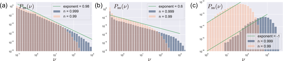
Figure 4: Numerical evaluation of the steady state PDF of the intensity $\hat{\nu}$ for the following parameter sets near the critical point: $n=0.999$ (blue bars) and $n=0.99$ (red bars). The theoretical power law is shown by the green straight line. (a) Background intensity $\nu_{0}=0.01$, relaxation time $\tau=1$, leading to the power-law exponent $0.98$. (b) $\nu_{0}=0.2$, $\tau=1$, leading to the power-law exponent $0.6$. (c) $\nu_{0}=1.0$, $\tau=1$, leading to the negative (i.e. growing) power-law exponent $-1.0$. For all simulations, the sampling time interval and total sampling time are $dt=0.001$ and $T_{\mathrm{tot}}=10000$ with the initial condition $\hat{z}(0)=0$. The initial 10% of the sample trajectories were discarded from the statistics.

We now present numerical confirmations of our theoretical prediction, in particular for the intermediate asymptotics as shown in Fig. 4. There is a well-developed literature on the numerical simulation of Hawkes process Harte2010 ; DassiosZhao13 . We have used an established simulation package for Python called “tick” (version 0.6.0.0) for 32-threads parallel computing. The total simulation time was $10^{4}$ seconds and the sampling time interval was $0.001$ second. We note that the initial 10% of the sampled trajectories were discorded for initialization.

For small background intensity $\nu_{0}\ll 1/\tau$, we obtain an approximate universal exponent $-1$. For $2\nu_{0}\tau<1$, we observe a decaying power law of exponent $1-2\nu_{0}\tau$, while we observe a growing power law for $2\nu_{0}\tau>1$. The power-law intermediate asymptotics is truncated by the exponential function, as predicted and also discussed in Ref. BouchaudTradebook2018 (albeit with the error of missing the $1$ in the exponent and thus failing to describe the intermediate asymptotics), ensuring the normalization of the PDF of the Hawkes intensities.

IV.1.2 Time-dependent solution

We now present the exact solution of the time-dependent master equation. In the Laplace representation, the dynamics of the PDF of the intensities is given by the following first-order PDE,

$$\frac{\partial\tilde{P}_{t}(s)}{\partial t}+\left(e^{-ns/\tau}-1+\frac{s}{\tau}\right)\frac{\partial\tilde{P}_{t}(s)}{\partial s}=\nu_{0}\left(e^{-ns/\tau}-1\right)\tilde{P}_{t}(s).$$ (55)

This equation can be solved by the method of characteristics (see Appendix C for a brief review). The corresponding Lagrange-Charpit equations are given by

$$\frac{ds}{dt}=e^{-ns/\tau}-1+\frac{s}{\tau},\>\>\>~{}~{}~{}~{}~{}~{}~{}~{}\frac{d\Phi}{dt}=\nu_{o}\left(e^{-ns/\tau}-1\right),~{}~{}~{}{\rm with}~{}~{}\Phi:=\log\tilde{P}~{}.$$ (56)

These equations can be solved explicitly,

$$t=\mathcal{F}(s)+C_{1},\>\>\>\>~{}~{}~{}~{}~{}~{}\Phi=\nu_{0}s-\frac{\nu_{0}}{\tau}\int_{0}^{s}\frac{s^{\prime}ds^{\prime}}{e^{-ns^{\prime}/\tau}-1+s^{\prime}/\tau}+C_{2}$$ (57)

with

$$\mathcal{F}(s):=\int_{s_{0}}^{s}\frac{ds^{\prime}}{e^{-ns^{\prime}/\tau}-1+s^{\prime}/\tau}+C_{1}.$$ (58)

$C_{1}$ and $C_{2}$ are constants of integration and $s_{0}$ is a positive constant chosen to satisfy several convenient properties discussed below.

Summary of the properties of $\mathcal{F}$.

We present several analytical properties of $\mathcal{F}(s)$ (see Appendix D for their proof):

1. $\mathcal{F}(s)$ is a monotonically increasing function by choosing $s_{0}>0$ appropriately.

2. The inverse function $\mathcal{F}^{-1}(s)$ can be defined uniquely.

In addition, for the sub-critical case $n<1$, the following properties hold true:

1. $s_{0}$ can be set to any positive value.

2. $\lim_{s\to+0}\mathcal{F}(s)=-\infty$.

3. $\lim_{s\to\infty}\mathcal{F}(s)=+\infty$.

4. $\mathcal{F}(s)$ can take all real values: $\mathcal{F}(s)\in(-\infty,\infty)$ for $s>0$.

Regularization of $\mathcal{F}(s)$.

In the following, we assume the sub-critical condition $n<1$. It is useful to decompose $\mathcal{F}(s)$ into regular and singular parts:

$$\mathcal{F}(s)=\int_{s_{0}}^{s}\frac{ds}{e^{-ns/\tau}-1+s/\tau}\underbrace{-\int_{s_{0}}^{s}\frac{ds}{(1-n)s/\tau}+\frac{\tau}{1-n}\log\frac{s}{s_{0}}}_{\mbox{totally zero as an identity}}=\underbrace{\frac{\tau}{1-n}\int_{s_{0}}^{s}ds\frac{1-e^{-ns/\tau}-ns/\tau}{s(e^{-ns/\tau}-1+s/\tau)}}_{\mbox{regular part}}+\underbrace{\frac{\tau}{1-n}\log\frac{s}{s_{0}}}_{\mbox{singular part}},$$ (59)

where the regular part is well-defined even for $s_{0}\to 0$. This expression is useful since the divergent factor in $\mathcal{F}(s)$ can be renormalized into the integral constant $C_{1}$, such that

$$C_{1}-\frac{\tau}{1-n}\log s_{0}\to C_{1}.$$ (60)

We then take the formal limit $s_{0}\to 0$ and use the following regularized expression for the sub-critical condition $n<1$,

$$\mathcal{F}(s)=\mathcal{F}_{\rm R}(s)+\frac{\tau}{1-n}\log s,\>\>\>\mathcal{F}_{\rm R}(s):=\frac{\tau}{1-n}\int_{0}^{s}ds\frac{1-e^{-ns/\tau}-ns/\tau}{s(e^{-ns/\tau}-1+s/\tau)},$$ (61)

where the $s_{0}$-dependence is removed as the result of the renormalization. The regular part has no singularity at $s\simeq 0$, and reads $\mathcal{F}_{\rm R}(s)\simeq-n^{2}s/\{2\tau(1-n)\}$.

Explicit solution.

Building on the above, we now provide the solution of the master equation (55). According to the method of characteristics (see Appendix. C for a brief review), the general solution is given by

$$C_{2}=\mathcal{H}(C_{1})$$ (62)

with an arbitrary function $\mathcal{H}(\cdot)$. The time-dependent solution $\log\tilde{Q}_{t}(s)=\log\tilde{P}_{t}(s)-\nu_{0}s$ is thus given by

$$\log\tilde{Q}_{t}(s)=-\frac{\nu_{0}}{\tau}\int_{0}^{s}\frac{sds}{e^{-ns/\tau}-1+s/\tau}+\mathcal{H}\left(t-\mathcal{F}(s)\right).$$ (63)

The function $\mathcal{H}(\cdot)$ is determined by the initial condition.

Let us assume that the initial PDF and its Laplace representation are given by $P_{t=0}(\nu)$ and $\tilde{P}_{t=0}(s)$, respectively. Then, we obtain

$$\mathcal{H}(-\mathcal{F}(s))=\log\tilde{P}_{t=0}(s)+\frac{\nu_{0}}{\tau}\int_{0}^{s}\frac{sds}{e^{-ns/\tau}-1+s/\tau}$$ (64)

or equivalently,

$$\mathcal{H}(x)=\log\tilde{P}_{t=0}\left(S(x)\right)+\frac{\nu_{0}}{\tau}\int_{0}^{S(x)}\frac{sds}{e^{-ns/\tau}-1+s/\tau},\>\>\>S(x)=\mathcal{F}^{-1}(-x).$$ (65)

Note that the time-dependent solution (63) is consistent with the steady solution (49)

$$\lim_{t\to\infty}\tilde{Q}_{t}(s)=\tilde{Q}_{\mathrm{ss}}(s),$$ (66)

since $\lim_{x\to+\infty}\mathcal{H}(x)=0$ (see Appendix. E.1 for the proof). We also note that, from the time-dependent solution  (63), we can derive the dynamics of the intensity $\hat{\nu}(t)$ for finite $t$ as

$$\langle\hat{\nu}(t)\rangle=\nu_{\rm ini}e^{-(1-n)t/\tau}+\nu_{0}\frac{1-e^{-nt/\tau}}{1-n}$$ (67)

with the initial condition $\hat{\nu}(0)=\nu_{\rm ini}$ (see Appendix. E.2 for the derivation). This expression (67) shows that the mean intensity converges at long times $t\to+\infty$ to $\langle\hat{\nu}(t)\rangle\to\nu_{0}/(1-n)$, which is a well-known result DalayVere03 ; HelmsSor02 . Expression (67) also shows that an initial impulse decays exponentially with a renormalised time decay $\tau/(1-n)$, which is also consistent with previous reports Escobar2015 . This diverging time scale $\tau/(1-n)$, as $n\to 1$, reflects the occurrence of all the generations of triggered events that renormalise the “bare” memory function into a “dressed” memory kernel with much longer memory.

Asymptotic relaxation dynamics for large $t$.

The time-dependent asymptotic solution is given for large $t$ by

$$\log\tilde{P}_{t}(s)\simeq-\frac{\nu_{0}}{\tau}\int_{S(t,s)}^{s}\frac{sds}{e^{-ns/\tau}-1+s/\tau}+\log\tilde{P}_{t=0}\left(S(t,s)\right),\>\>\>S(t,s)=s\exp\left[-\frac{1-n}{\tau}\left(t-\mathcal{F}_{\rm R}(s)\right)\right],$$ (68)

assuming that $t\gg\mathcal{F}(s)$ for a given $s$. As a corollary of this formula, an asymptotic prediction for the distribution conditional on the initial intensity is given by the following formula

$$P(\nu,t|\nu_{\rm ini},t=0)=\mathcal{L}^{-1}_{1}\left[\tilde{P}_{t}(s);t\right],\>\>\>\log\tilde{P}_{t=0}(s)=-\nu_{\rm ini}s$$ (69)

for large $t$. Note that asymptotic convergence of these formula is not uniform in terms of $s$; indeed, the convergence of the Laplace representation for large $s$ is slower than that for small $s$.

IV.1.3 Another derivation of the power law exponent: linear stability analysis of the Lagrange-Charpit equation

We have presented both the steady state and time-dependent solutions of the master equations, based on exact or asymptotic methods. While these formulations are already clear, here we revisit the power-law bahavior (53) of the steady state PDF, and present another derivation based on the linear stability analysis of the Lagrange-Charpit equation, which has the advantage of being generalisable to memory kernels defined as superposition of exponential functions. Indeed, while the derivation based on the exact solution (49) is clear and powerful, it is not easy to extend this kind of calculation to general cases, such as superposition of exponential kernels. In contrast, the derivation that we now present can be extended to arbitrary forms of the memory kernel of the Hawkes processes, as will be shown later. Moreover, we have found additional distinct derivations of (53) and we refer the interested reader to Appendix. B.

While the steady state master equation (48) is a ordinary differential equation which can be solved exactly, let us consider its corresponding Lagrange-Charpit equations,

$$\frac{ds}{dl}=-e^{-ns/\tau}+1-\frac{s}{\tau},\>\>\>\frac{d}{dl}\log\tilde{P}_{\mathrm{ss}}=-\nu_{0}\left(e^{-ns/\tau}-1\right)$$ (70)

where we introduce the parameter $l$ of the characteristic curve. These equations can be regarded as describing a “dynamical system” in terms of the auxiliary “time” $l$. This formulation is useful because the well-developed theory of dynamical systems is applicable even to more general cases as shown later.

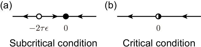
Figure 5: Schematic illustration of the vector field $V(s):=ds/dt=-e^{-ns/\tau}+1-s/\tau$ along the $s$ dimension as a function of “time” $l$. (a) Near critical condition $\epsilon:=1-n\ll 1$, two fixed points exist at $s=0$ (attractor) and $s\simeq-2\tau\epsilon$ (repeller). (b) At the critical condition $n=1$, the repeller merges with the attractor, which corresponds to a transcritical bifurcation.

Sub-critical condition $n<1$.

Let us first focus on the sub-critical case $n<1$ and consider the expansion of equations (70) around $s=0$, which leads to

$$\frac{ds}{dl}\simeq-\frac{1-n}{\tau}s-\frac{n^{2}s^{2}}{2\tau^{2}}+\dots,\>\>\>\frac{d}{dl}\log\tilde{P}_{\mathrm{ss}}\simeq\frac{n\nu_{0}}{\tau}s+\dots.$$ (71)

The corresponding flow of this effective dynamical system $s(l)$ along the $s$ axis as a function of “time” $l$ is illustrated in Fig. 5. Near the critical condition $\epsilon=1-n\ll 1$, this “dynamical system” has two fixed points $V(s)=0$ at

$$s=0,\>\>\>s\simeq-2\tau\epsilon$$ (72)

The former is a stable attractor whereas the latter is an unstable repeller (see Fig. 5a). Remarkably, the critical condition $n=1$ for the Hawkes process corresponds to the condition of a transcritical bifurcation (i.e., the repeller merges with the attractor; see Fig. 5b) for the “dynamical system” described by the Lagrange-Charpit equations. This picture is useful because it can be straightforwardly generalized to more general memory kernels $h(t)$, as shown later.

Let us neglect the sub-leading contribution to obtain the general solution as

$$s=e^{-(1-n)(l-l_{0})/\tau},\>\>\>\log\tilde{P}_{\mathrm{ss}}\simeq\frac{n\nu_{0}}{\tau}\int dl~{}s(l)+C$$ (73)

with constants of integration $l_{0}$ and $C$. In the following, we set the initial “time” (i.e., the initial point on the characteristic curve) as $l_{0}=0$. We then obtain

$$\log\tilde{P}_{\mathrm{ss}}\simeq-\frac{n\nu_{0}s}{1-n}+C$$ (74)

with constant of integration $C$. This constant is fixed by the condition of normalization of the PDF, given by $\log\tilde{P}_{\mathrm{ss}}=0$ for $s=0$, which imposes $C=0$. We thus obtain

$$\log\tilde{Q}_{\mathrm{ss}}(s)=-\nu_{0}s+\log\tilde{P}_{\mathrm{ss}}(s)\simeq-\frac{\nu_{0}s}{1-n},$$ (75)

which is consistent with the asymptotic mean intensity in the steady state (see the long time limit of Eq. (67)).

At criticality $n=1$.

For $n=1$, the lowest-order contribution in the Lagrange-Charpit equation is given by

$$\frac{ds}{dl}\simeq-\frac{s^{2}}{2\tau^{2}}\>\>\>\Longrightarrow\>\>\>s=\frac{2\tau^{2}}{l-l_{0}}.$$ (76)

with constant of integration $l_{0}$. In the following, we set $l_{0}=0$ as the initial point on the characteristic curve. We then obtain

$$\log\tilde{P}_{\mathrm{ss}}=\frac{\nu_{0}}{\tau}\int dl~{}s(l)+C\simeq-2\nu_{0}\tau\log|s|+C$$ (77)

with the constant of integration $C$. The constant is an “divergent” constant since it has to compensate the diverging logarithm to ensure that $\log P_{\mathrm{ss}}(s=0)=0$. This “divergent” constant appears as a result of neglecting the ultra-violet (UV) cutoff for small $s$ (which corresponds to neglecting the exponential tail of the PDF of intensities). By ignoring the divergent constant $C$, we obtain the intermediate asymptotics,

$$P_{\mathrm{ss}}(\nu)\propto\nu^{-1+2\nu_{0}\tau},$$ (78)

which recovers the leading power law intermediate asymptotic (53), which is a special case of the general solution (47).

IV.2 Double exponential kernel

We now consider the case where the memory function (24) is made of $K=2$ exponential functions. Since the Laplace representation of the master equation is still a first-order partial differential equation, its solution can be formally obtained by the method of characteristics (see Appendix. C for a short review). Unfortunately, the time-dependent Lagrange Charpit equation cannot be exactly solved in explicit form anymore. We therefore focus on the steady state solution of the master equation, with a special focus on the regime close to the critical point. We develop the stability analysis of the Lagrange-Charpit equations following the same approach as in Sec. IV.1.3.

Let us start from the Lagrange-Charpit equations, which are given by

$$\frac{ds_{1}}{dl} =-e^{-(n_{1}s_{1}/\tau_{1}+n_{2}s_{2}/\tau_{2})}+1-\frac{s_{1}}{\tau_{1}},$$ (79a)

$$\frac{ds_{2}}{dl} =-e^{-(n_{1}s_{1}/\tau_{1}+n_{2}s_{2}/\tau_{2})}+1-\frac{s_{2}}{\tau_{2}},$$ (79b)

$$\frac{d\Phi}{dl} =-\nu_{0}\left(e^{-(n_{1}s_{1}/\tau_{1}+n_{2}s_{2}/\tau_{2})}-1\right)~{}~{}~{}~{}~{}{\rm with}~{}~{}\Phi:=\log\tilde{P}_{\mathrm{ss}}$$ (79c)

and $l$ is the auxiliary “time” parameterising the position on the characteristic curve. Let us develop the stability analysis around $s=0$ (i.e. for large $\nu$’s) for this pseudo dynamical system.

Sub-critical case $n<1$.

Assuming $n:=n_{1}+n_{2}<1$, let us first consider the linearized dynamics of system (79) as

$$\frac{d\bm{s}}{dl}\simeq-\bm{H}\bm{s},\>\>\>\frac{d\Phi}{dl}\simeq\nu_{0}\bm{K}\bm{s}$$ (80)

with

$$\bm{s}:=\begin{pmatrix}s_{1}\\ s_{2}\end{pmatrix},\>\>\>\bm{H}:=\begin{pmatrix}\frac{1-n_{1}}{\tau_{1}}&\frac{-n_{2}}{\tau_{2}}\\ \frac{-n_{1}}{\tau_{1}}&\frac{1-n_{2}}{\tau_{2}}\end{pmatrix},\>\>\>\bm{K}:=\begin{pmatrix}\frac{n_{1}}{\tau_{1}},\frac{n_{2}}{\tau_{2}}\end{pmatrix}.$$ (81)

Regarding this system as a dynamical system with the auxiliary “time” $l$, its qualitative dynamics can be illustrated by its phase space depicted in Fig. 6. In the subcritical case $n<1$, the origin $\bm{s}=(0,0)$ is “attractive” since all the eigenvalues of $\bm{H}$ are positive (Fig. 6a).

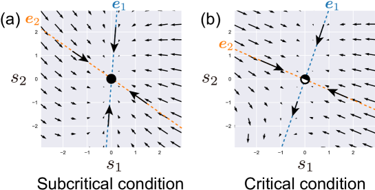
Figure 6: Qualitative representation of the Lagrange-Charpit equations in phase space. By rewriting $d\bm{s}/dk:=\bm{V}(\bm{s})\simeq-\bm{H}\bm{s}$, the “velocity” vector field $\bm{V}(\bm{s})$ is plotted in the phase space $(s_{1},s_{2})$. (a) Subcritical case with $(\tau_{1},\tau_{2},n_{1},n_{2})=(1,3,0.3,0.1)$, showing that $\bm{s}=\bm{0}$ is a stable attractor. (b) Critical case with $(\tau_{1},\tau_{2},n_{1},n_{2})=(1,3,0.3,0.7)$, showing that the $\bm{e}_{1}$ direction is marginal in terms of the linear stability analysis (i.e., the repeller merges with the attractor, which corresponds to a transcritical bifurcation in dynamical systems).

Let us introduce the eigenvalues $\lambda_{1},\lambda_{2}$ and eigenvectors $\bm{e}_{1},\bm{e}_{2}$ of $\bm{H}$, such that

$$\bm{P}:=\begin{pmatrix}\bm{e}_{1},\bm{e}_{2}\end{pmatrix},\>\>\>\bm{P}^{-1}\bm{H}\bm{P}=\begin{pmatrix}\lambda_{1}&0\\ 0&\lambda_{2}\end{pmatrix}.$$ (82)

Because all eigenvalues are real (see Appendix. F.1 for the proof), we denote $\lambda_{1}\leq\lambda_{2}$. The determinant of $\bm{H}$ is given by

$$\det\bm{H}=\frac{1-n}{\tau_{1}\tau_{2}}.$$ (83)

This means that the zero eigenvalue $\lambda_{1}=0$ appears at the critical point $n=1$. Below the critical point $n<1$, all the eigenvalues are positive ($\lambda_{1},\lambda_{2}>0$). For $n<1$, the dynamics can be rewritten as

$$\frac{d}{dl}\bm{P}^{-1}\bm{s}=-\begin{pmatrix}\lambda_{1}&0\\ 0&\lambda_{2}\end{pmatrix}\bm{P}^{-1}\bm{s}\>\>\>\Longrightarrow\>\>\>\bm{s}(l)=\bm{P}\begin{pmatrix}e^{-\lambda_{1}(l-l_{0})}\\ e^{-\lambda_{2}(l-l_{0})}/C_{1}\end{pmatrix}$$ (84)

with constants of integration $l_{0}$ and $C_{1}$. We can assume $l_{0}=0$ as the initial point of the characteristic curve without loss of generality. Integrating the second equation in (80), we obtain

$$\Phi=\nu_{0}\bm{K}\int\bm{s}(l)dl+C_{2}=-\nu_{0}\bm{K}\bm{P}\begin{pmatrix}1/\lambda_{1}&0\\ 0&1/\lambda_{2}\end{pmatrix}\bm{P}^{-1}\bm{s}+C_{2}=-\nu\bm{K}\bm{H}^{-1}\bm{s}+C_{2}.$$ (85)

The general solution is given by

$$\mathcal{H}(C_{1})=C_{2}$$ (86)

with a function $\mathcal{H}$ determined by the initial condition on the characteristic curve. Let us introduce

$$\bar{s}:=\bm{P}^{-1}\bm{s}=\begin{pmatrix}\bar{s}_{1}\\ \bar{s}_{2}\end{pmatrix}\>\>\>\Longrightarrow\>\>\>C_{1}=\left(\bar{s}_{1}\right)^{\lambda_{2}/\lambda_{1}}\left(\bar{s}_{2}\right)^{-1}.$$ (87)

This means that the solution is given by the following form:

$$\Phi(\bm{s})=-\nu\bm{K}\bm{H}^{-1}\bm{s}+\mathcal{H}\left(\left(\bar{s}_{1}\right)^{\lambda_{2}/\lambda_{1}}\left(\bar{s}_{2}\right)^{-1}\right).$$ (88)

Because of the renormalization of the PDF, the following relation must hold

$$\lim_{\bm{s}\to\bm{0}}\Phi(\bm{s})=0$$ (89)

for any path in the $(s_{1},s_{2})$ space ending on the origin (limit $\bm{s}\to\bm{0}$). Let us consider the specific limit such that $\bar{s}_{1}\to 0$ with $\bar{s}_{2}=x^{-1}(\bar{s}_{1})^{\lambda_{2}/\lambda_{1}}$ for an arbitrary positive $x$:

$$\lim_{\bar{s}_{1}\to 0}\Phi(\bm{s})=\mathcal{H}(x).$$ (90)

Since the left-hand side (LHS) is zero for any $x$, the function $\mathcal{H}(\cdot)$ must be identically zero. With $\Phi:=\log\tilde{P}_{\mathrm{ss}}$ as defined in (79), this leads to

$$\log\tilde{P}_{\mathrm{ss}}(\bm{s})=-\nu\bm{K}\bm{H}^{-1}\bm{s}.$$ (91)

By substituting with the special $\bm{s}=(s_{1}=s,s_{2}=s)^{\rm{T}}$, we obtain

$$\log\tilde{Q}_{\mathrm{ss}}(s)=-\nu_{0}s+\Phi_{t=\infty}\left(s(1,1)^{\rm{T}}\right)\simeq-\frac{\nu_{0}}{1-n}s$$ (92)

for small $s$, which recovers expression (75) derived above.

Critical case $n=1$.

In this case, the eigenvalues and eigenvectors of $\bm{H}$ are given by

$$\lambda_{1}=0,\>\>\>\lambda_{2}=\frac{n_{1}\tau_{1}+n_{2}\tau_{2}}{\tau_{1}\tau_{2}},\>\>\>\bm{e}_{1}=\begin{pmatrix}\tau_{1}\\ \tau_{2}\end{pmatrix},\>\>\>\bm{e}_{2}=\begin{pmatrix}-n_{2}\\ n_{1}\end{pmatrix}.$$ (93)

This means that the eigenvalue matrix and its inverse matrix are respectively given by

$$\bm{P}=\begin{pmatrix}\tau_{1}&-n_{2}\\ \tau_{2}&n_{1}\end{pmatrix},\>\>\>\bm{P}^{-1}=\frac{1}{\alpha}\begin{pmatrix}n_{1}&n_{2}\\ -\tau_{2}&\tau_{1}\end{pmatrix},\>\>\>\alpha:=\det\bm{P}=\tau_{1}n_{1}+\tau_{2}n_{2}$$ (94)

This value of $\alpha$ is the special case for two exponentials of the general definition (34). Accordingly, let us introduce

$$\bm{X}=(X,Y)^{\rm{T}}=\bm{P}^{-1}\bm{s},\>\>\>\Longleftrightarrow\>\>\>X=\frac{n_{1}s_{1}+n_{2}s_{2}}{\alpha},\>\>\>Y=\frac{-\tau_{2}s_{1}+\tau_{1}s_{2}}{\alpha}.$$ (95)

We then obtain

$$\frac{dX}{dl}=0,\>\>\>\frac{dY}{dl}=-\lambda_{2}Y$$ (96)

at the leading linear order in expansions in powers of $X$ and $Y$. Since the first linear term is zero in the dynamics of $X$, corresponding to a transcritical bifurcation for the Lagrange-Charpit equations (79), we need to take into account the second order term in $X$, namely

$$e^{-(n_{1}s_{1}/\tau_{1}+n_{2}s_{2}/\tau_{2})}\simeq 1-X+\frac{X^{2}}{2}+n_{1}n_{2}\left(\frac{1}{\tau_{1}}-\frac{1}{\tau_{2}}\right)Y+O(XY,X^{2}Y,Y^{2})$$ (97)

where we have dropped terms of the order $Y^{2}$, $XY$ and $X^{2}Y$. We then obtain the dynamical equations at the transcritical bifurcation (see Fig. 6b) to leading-order

$$\frac{dY}{dl}\simeq-\lambda_{2}Y,\>\>\>\frac{dX}{dl}\simeq-\frac{X^{2}}{2\alpha}$$ (98)

whose solutions are given by

$$X(l)=\frac{2\alpha}{l-l_{0}},\>\>\>Y(l)=C_{1}e^{-\lambda_{2}(l-l_{0})}$$ (99)

with constants of integration $l_{0}$ and $C_{1}$. We can assume $l_{0}=0$ as the initial point on the characteristic curve. Remarkably, only the contribution along the $X$ axis is dominant for the large $l$ limit (i.e., $|X|\gg|Y|$ for $l\to\infty$), which corresponds to the asymptotic limit $\bm{s}\to 0$. We then obtain

$$\Phi\simeq\nu_{0}\int dl\left(\frac{n_{1}s_{1}(l)}{\tau_{1}}+\frac{n_{2}s_{2}(l)}{\tau_{2}}\right)\simeq-2\nu_{0}\alpha\log|X|+\frac{\nu_{0}n_{1}n_{2}}{\lambda_{2}}\left(\frac{1}{\tau_{1}}-\frac{1}{\tau_{2}}\right)Y+C_{2}$$ (100)

with constant of integration $C_{2}$. The general solution is given by

$$\mathcal{H}(C_{1})=C_{2}$$ (101)

with a function $\mathcal{H}$, which is determined by the initial condition. Considering that

$$C_{1}=Y\exp\left[\frac{2\lambda_{2}\alpha}{X}\right],$$ (102)

the solution is given by the following form:

$$\Phi(\bm{s})=-2\nu_{0}\alpha\log|X|+\frac{\nu_{0}n_{1}n_{2}}{\lambda_{2}}\left(\frac{1}{\tau_{1}}-\frac{1}{\tau_{2}}\right)Y+\mathcal{H}\left(Y\exp\left[\frac{2\lambda_{2}\alpha}{X}\right]\right).$$ (103)

Because we have neglected the UV cutoff for small $s$, there is an artificial divergent term $-2\nu_{0}\alpha\log|X|$ for small $X$. Except for this divergent term, $\Phi(\bm{s})$ must be constant for $s\to 0$. The function $\mathcal{H}(\cdot)$ is thus constant because

$$\lim_{y\to 0}\left[\Phi(\bm{s})+2\nu_{0}\alpha\log|X|\right]=\mathcal{H}(Z)=\mbox{const.}$$ (104)

with the choice of $X=2\lambda_{2}\alpha/\log(Z/Y)$ for any positive constant $Z$. Therefore, we obtain the steady solution

$$\log\tilde{P}_{\mathrm{ss}}(\bm{s})\simeq-2\nu_{0}\alpha\log|X|+\frac{\nu_{0}n_{1}n_{2}}{\lambda_{2}}\left(\frac{1}{\tau_{1}}-\frac{1}{\tau_{2}}\right)Y$$ (105)

for small $X$ and $Y$, by ignoring the UV cutoff and the constant contribution. This recovers the power law formula of the intermediate asymptotics of the PDF of the Hawkes intensities:

$$\log\tilde{Q}_{\mathrm{ss}}(s):=-\nu_{0}s+\log\tilde{P}_{\mathrm{ss}}(s,s)\simeq-2\nu_{0}\alpha\log|s|\>\>\>(s\sim 0)\>\>\>\Longleftrightarrow\>\>\>P(\nu)\sim\nu^{-1+2\nu_{0}\alpha}\>\>\>(\nu\to+\infty),$$ (106)

with $\alpha=\tau_{1}n_{1}+\tau_{2}n_{2}$ as defined in (94).

Numerical verification.

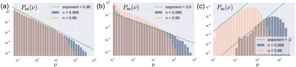
Figure 7: Numerical evaluation of the steady state PDF of the Hawkes intensity $\hat{\nu}$ for the double exponential case $K=2$ (24) with $(\tau_{1},\tau_{2})=(1,3)$, $(n_{1},n_{2})=(0.5,0.499)$ or $(n_{1},n_{2})=(0.5,0.49)$, near the critical point: (a) Background intensity $\nu_{0}=0.01$, leading to the power law exponent $0.96$. (b) $\nu_{0}=0.1$, leading to the power law exponent $0.6$. (c) $\nu_{0}=0.75$, leading to the negative (i.e. growing PDF) power law exponent $-2.0$. For all simulations, the sampling time interval and total sampling time are $dt=0.001$ and $T_{\mathrm{tot}}=10000$ from the initial condition $\hat{z}(0)=0$. The initial 10% of the sample was discarded from the statistics.

We have numerically confirmed our theoretical prediction (106), a special case of (47) for a memory kernel with two exponentials, as shown in Fig. 7. The main properties are the same as those shown in Fig. 4, implying that our prediction is verified for memory kernels with one and two exponentials.

IV.3 Discrete superposition of exponential kernels

We now consider the case where the memory kernel is the sum of an arbitrary finite number $K$ of exponentials according to expression (24). Our treatment follows the method presented for the case $K=2$.

The corresponding Lagrange-Charpit equations read:

$$\frac{ds_{k}}{dl}=-e^{-\sum_{j=1}^{K}n_{j}s_{j}/\tau_{j}}+1-\frac{s_{k}}{\tau_{k}},\>\>\>~{}~{}~{}~{}~{}~{}\frac{d\Phi}{dl}=-\nu_{0}\left(e^{-\sum_{j=1}^{K}n_{j}s_{j}/\tau_{j}}-1\right).$$ (107)

The derivation of the PDF of the Hawkes intensities boils down to a stability analysis of these equations around $s=0$ in the neighbourhood of the critical condition $n=1$.

Sub-critical case $n<1$.

We linearize the Lagrange-Charpit equations to obtain

$$\frac{d\bm{s}}{dl}\simeq-\bm{H}\bm{s},\>\>\>\frac{d\Phi}{dl}\simeq\nu_{0}\bm{K}\bm{s}$$ (108)

with

$$\bm{H}:=\begin{pmatrix}\frac{1-n_{1}}{\tau_{1}},&-\frac{n_{2}}{\tau_{2}},&\dots&-\frac{n_{K}}{\tau_{K}}\\ -\frac{n_{1}}{\tau_{1}},&\frac{1-n_{2}}{\tau_{2}},&\dots&-\frac{n_{K}}{\tau_{K}}\\ \vdots&\vdots&\ddots&\vdots\\ -\frac{n_{1}}{\tau_{1}},&-\frac{n_{2}}{\tau_{2}},&\dots&\frac{1-n_{K}}{\tau_{K}}\end{pmatrix},\>\>\>\bm{K}:=\left(\frac{n_{1}}{\tau_{1}},\dots,\frac{n_{K}}{\tau_{K}}\right).$$ (109)

Considering that all eigenvalues $\{\lambda_{k}\}_{k=1,\dots,K}$ of $\bm{H}$ are real (see Appendix. F.1 for its proof), we order them according to $\lambda_{i}<\lambda_{j}$ for $i<j$. We denote the corresponding eigenvectors as $\{\bm{e}_{k}\}_{k=1,\dots,K}$. The matrix $\bm{H}$ can thus be diagonalised as follows

$$\bm{P}:=(\bm{e}_{1},\dots,\bm{e}_{K}),\>\>\>\bm{P}^{-1}\bm{H}\bm{P}=\begin{pmatrix}\lambda_{1},&0,&\dots&0\\ 0,&\lambda_{2},&\dots&0\\ \vdots&\vdots&\ddots&\vdots\\ 0,&0,&\dots&\lambda_{K}\end{pmatrix}.$$ (110)

The critical case $n=1$ corresponds to the existence of a zero eigenvalue. Therefore, at the critical point, the determinant of $\bm{H}$ is zero (see Appendix. F.2 for the derivation of the explicit form of its determinant):

$$\det\bm{H}=\frac{1-\sum_{k=1}^{K}n_{k}}{\prod_{k=1}^{K}\tau_{k}}=0\>\>\>\>\Longleftrightarrow\>\>\>\>n:=\sum_{k=1}^{K}n_{k}=1.$$ (111)

Following calculations similar those presented in to Sec. IV.2, we obtain

$$\Phi(\bm{s})\simeq-\nu_{0}\bm{K}\bm{H}^{-1}\bm{s}$$ (112)

where the inverse matrix $\bm{H}^{-1}$ is explicitly given in Appendix. F.3. We finally obtain

$$\log\tilde{Q}_{\mathrm{ss}}(s)=-\nu_{0}s+\Phi(s(1,\dots,1)^{T})=\frac{-\nu_{0}}{1-n}s,$$ (113)

again recovering (92) and (75) derived above.

Critical case $n=1$.

At the critical point, the smallest eigenvalue of $\bm{H}$ is zero ($\lambda_{1}=0$). By direct substitution, its corresponding eigenvector is

$$\bm{e}_{1}=(\tau_{1},\dots,\tau_{K})^{T}~{},$$ (114)

as seen from

$$\bm{H}\bm{e}_{1}=\begin{pmatrix}\frac{1-n_{1}}{\tau_{1}},&-\frac{n_{2}}{\tau_{2}},&\dots&-\frac{n_{K}}{\tau_{K}}\\ -\frac{n_{1}}{\tau_{1}},&\frac{1-n_{2}}{\tau_{2}},&\dots&-\frac{n_{K}}{\tau_{K}}\\ \vdots&\vdots&\ddots&\vdots\\ -\frac{n_{1}}{\tau_{1}},&-\frac{n_{2}}{\tau_{2}},&\dots&\frac{1-n_{K}}{\tau_{K}}\end{pmatrix}\begin{pmatrix}\tau_{1}\\ \tau_{2}\\ \vdots\\ \tau_{K}\end{pmatrix}=\begin{pmatrix}1-n\\ 1-n\\ \vdots\\ 1-n\end{pmatrix}=\bm{0}~{}~{}~{}~{}~{}{\rm for}~{}n=1.$$ (115)

We now introduce a new set of variables (i.e., representation based on the eigenvectors)

$$\bm{X}=\begin{pmatrix}X_{1}\\ X_{2}\\ \dots\\ X_{K}\end{pmatrix}:=\bm{P}^{-1}\bm{s},\>\>\>\>~{}~{}~{}~{}~{}\bm{P}^{-1}=\begin{pmatrix}\bm{g}_{1}^{T}\\ \bm{g}_{2}^{T}\\ \dots\\ \bm{g}_{K}^{T}\end{pmatrix}\bm{s}.$$ (116)

The linearized Lagrange-Charpit equations are given by

$$\frac{dX_{1}}{dl}\simeq 0,\>\>\>~{}~{}~{}~{}\frac{dX_{j}}{dl}\simeq-\lambda_{j}X_{j}~{}~{}~{}~{}{\rm for}~{}j\geq 2~{}.$$ (117)

Similarly to Eq. (99), the leading-order contribution comes from the $X_{1}$ direction because $|X_{1}|\gg|X_{j}|$ for $j\geq 2$ in the asymptotic limit $l\to\infty$. We thus neglect other contribution by assuming $X_{j}\sim 0$ for $j\geq 1$. It is therefore necessary to take the second-order contribution along the $X_{1}$ direction,

$$e^{-\sum_{k=1}^{K}n_{k}s_{k}/\tau_{k}}-1=-\sum_{k=1}^{K}\frac{n_{k}s_{k}}{\tau_{k}}+\frac{1}{2}\left(\sum_{k=1}^{K}\frac{n_{k}s_{k}}{\tau_{k}}\right)^{2}+\dots.$$ (118)

We note that $X_{1}$ is given by

$$X_{1}=\bm{g}_{1}\cdot\bm{s}=\frac{1}{\alpha}\sum_{k=1}^{K}n_{k}s_{k},\>\>\>~{}~{}~{}~{}~{}\bm{g}_{1}=\left(\frac{n_{1}}{\alpha},\dots,\frac{n_{K}}{\alpha}\right)^{T},$$ (119)

where $\alpha:=\sum_{k=1}^{K}\tau_{k}n_{k}$, which is a special case for a discrete sum of exponentials of the general definition (34).

Taking the derivative of (119) and using equation (107), we obtain

$$\frac{dX_{1}}{dl}=\frac{1}{\alpha}\sum_{k=1}^{K}n_{k}\frac{ds_{k}}{dl}=0-\frac{1}{2\alpha}\left(\sum_{k=1}^{K}\frac{n_{k}s_{k}}{\tau_{k}}\right)^{2}+\dots.$$ (120)

This means that $\bm{g}_{1}$ is a correct representation. Note that the value of $\alpha$ given by (34) ensures consistency with the following identify:

$$\bm{P}^{-1}\bm{P}=\begin{pmatrix}\bm{g}_{1}^{T}\\ \bm{g}_{2}^{T}\\ \dots\\ \bm{g}_{K}^{T}\end{pmatrix}\begin{pmatrix}\bm{e}_{1},\bm{e}_{2},\dots,\bm{e}_{K}\end{pmatrix}=\begin{pmatrix}n_{1}/\alpha,&n_{2}/\alpha,&\dots&n_{K}/\alpha\\ \bigcirc,&\bigcirc,&\dots&\bigcirc\\ \vdots&\vdots&\ddots&\vdots\\ \bigcirc,&\bigcirc,&\dots&\bigcirc\end{pmatrix}\begin{pmatrix}\tau_{1},&\bigcirc,&\dots&\bigcirc\\ \tau_{2},&\bigcirc,&\dots&\bigcirc\\ \vdots&\vdots&\ddots&\vdots\\ \tau_{2},&\bigcirc,&\dots&\bigcirc\end{pmatrix}=\begin{pmatrix}1,&0,&\dots&0\\ 0,&1,&\dots&0\\ \vdots&\vdots&\ddots&\vdots\\ 0,&0,&\dots&1\end{pmatrix},$$ (121)

where $\bigcirc$ represents some unspecified value. Since the contribution of $X_{2},\dots X_{K}$ can be ignored for the description of the leading behavior along $X_{1}$, let us set $X_{2}=X_{3}=\dots=X_{K}=0$, which leads

$$\bm{s}=\bm{P}\bm{X}\simeq(\bm{e}_{1},\dots,\bm{e}_{K})\begin{pmatrix}X_{1}\\ 0\\ \vdots\\ 0\end{pmatrix}=X\bm{e}_{1}=\begin{pmatrix}X_{1}\tau_{1}\\ X_{1}\tau_{2}\\ \vdots\\ X_{1}\tau_{K}\end{pmatrix}.$$ (122)

We thus obtain the second-order contribution along the $X_{1}$ axis by ignoring nonlinear contribution from $X_{2},\dots,X_{K}$:

$$\frac{dX_{1}}{dl}\simeq-\frac{X_{1}^{2}}{2\alpha}.$$ (123)

With calculations that follow step by step those in Sec. IV.2, we obtain

$$\log\tilde{Q}_{\mathrm{ss}}(s)\simeq-2\nu_{0}\alpha\log|s|\>\>\>\Longleftrightarrow\>\>\>P(\nu)\sim\nu^{-1+2\nu_{0}\alpha},\>\>\>{\rm with}~{}\alpha:=\sum_{k=1}^{K}n_{k}\tau_{k}.$$ (124)

This recovers the power law formula of the intermediate asymptotics of the PDF of the Hawkes intensities given by (47).

IV.4 General case

We are now prepared to study the general case where the memory kernel of the Hawkes process is a continuous superposition of exponential functions (33). Introducing the steady state cumulant functional

$$\Phi[s]:=\log\tilde{P}_{\mathrm{ss}}[s],$$ (125)

and from the master equation in its functional Laplace representation Eq. (45), we obtain the following first-order functional differential equation in the steady state,

$$\int_{0}^{\infty}dx\left(e^{-\int_{0}^{\infty}dx^{\prime}s(x^{\prime})n(x^{\prime})/x^{\prime}}-1+\frac{s(x)}{x}\right)\frac{\delta\Phi[s]}{\delta s(x)}=\nu_{0}\left(e^{-\int_{0}^{\infty}dx^{\prime}s(x^{\prime})n(x^{\prime})/x^{\prime}}-1\right).$$ (126)

The corresponding Lagrange-Charpit equations are the following partial-integro equations,

$$\frac{\partial s(l;x)}{\partial l}=1-e^{-\int_{0}^{\infty}dx^{\prime}s(x^{\prime})n(x^{\prime})/x^{\prime}}-\frac{s(x)}{\tau},\>\>\>\>\frac{\partial\Phi(l)}{\partial l}=-\nu_{0}\left(e^{-\int_{0}^{\infty}dx^{\prime}s(x^{\prime})n(x^{\prime})/x^{\prime}}-1\right)$$ (127)

where $l$ is the curvilinear parameter indexing the position along the characteristic curve. We now perform the stability analysis of this equation (127) in the neighbourhood of $s=0$ close to the critical condition $n=1$.

Sub-critical case $n<1$.

We linearize the Lagrange-Charpit equation (127) to obtain

$$\frac{\partial s(l;x)}{\partial l}=-\int_{0}^{\infty}dx^{\prime}H(x,x^{\prime})s(x^{\prime}),\>\>\>\>\frac{\partial\Phi(l)}{\partial l}=\nu_{0}\int_{0}^{\infty}dx^{\prime}K(x^{\prime})s(x^{\prime})$$ (128)

with

$$H(x,x^{\prime}):=\frac{\delta(x-x^{\prime})-n(x^{\prime})}{x^{\prime}},\>\>\>\>K(x^{\prime}):=\frac{n(x^{\prime})}{x^{\prime}}.$$ (129)

Let us introduce the eigenvalues $\lambda\geq\lambda_{\min}$ and eigenfunctions $e(x;\lambda)$, satisfying

$$\int_{0}^{\infty}dx^{\prime}H(x,x^{\prime})e(x^{\prime};\lambda)=\lambda e(x;\lambda).$$ (130)

Appendix  G.1 shows that all the eigenvalues are real. The inverse matrix of $H(x,x^{\prime})$, denoted by $H^{-1}(x,x^{\prime})$, can be explicitly obtained as shown in Appendix G.2. Since the inverse matrix $H^{-1}(x,x^{\prime})$ has a singularity at $n=1$, the critical condition of this Hawkes process is given by $n=1$ as expected. Using calculations that are analogous to those in Sec. IV.2, we obtain

$$\Phi[s]\simeq-\nu_{0}\int_{0}^{\infty}dx\int_{0}^{\infty}dx^{\prime}K(x)H^{-1}(x,x^{\prime})s(x^{\prime}),$$ (131)

from which we state that

$$\log\tilde{Q}_{\mathrm{ss}}(s)=-\nu_{0}s+\Phi[s\bm{1}(x)]=\frac{-\nu_{0}}{1-n}s.$$ (132)

where $\bm{1}(x)$ is an indicator function defined by $\bm{1}(x)=1$ for any $x$. This recovers (75), (92) and (113) derived above.

Critical case $n=1$.

At criticality, the smallest eigenvalue vanishes: $\lambda_{\min}=0$. Indeed, we obtain the zero eigenfunction

$$e(x;\lambda=0)=x,$$ (133)

which can be checked by direct substitution:

$$\int_{0}^{\infty}dxH(x,x^{\prime})e(x^{\prime};\lambda=0)=\int_{0}^{\infty}dx\frac{\delta(x-x^{\prime})-n(x^{\prime})}{x^{\prime}}x^{\prime}=1-n=0~{},~{}~{}{\rm for}~{}n=1.$$ (134)

We now introduce a set of variables to obtain a new representation based on the eigenfunctions,

$$s(x)=\sum_{\lambda}e(x;\lambda)X(\lambda)\>\>\>\Longleftrightarrow\>\>\>X(\lambda)=\int_{0}^{\infty}dxe^{-1}(\lambda;x)s(x)$$ (135)

with the inverse matrix $e^{-1}(\lambda;x)$ satisfying

$$\int_{0}^{\infty}dxe^{-1}(\lambda;x)e(x;\lambda^{\prime})=\delta_{\lambda,\lambda^{\prime}}.$$ (136)

We assume the existence of the inverse matrix, which is equivalent to the assumption that the set of all eigenfunctions is complete. $H(x,x^{\prime})$ can be diagonalized:

$$\int_{0}^{\infty}dx\int_{0}^{\infty}dx^{\prime}e^{-1}(\lambda;x)H(x,x^{\prime})e(x^{\prime};\lambda^{\prime})=\lambda\delta_{\lambda,\lambda^{\prime}}.$$ (137)

We then obtain the linearized Lagrange-Charpit equations,

$$\frac{\partial X(\lambda)}{\partial l}\simeq-\lambda X(\lambda).$$ (138)

The dominant contribution comes from the vanishing eigenvalue. We therefore focus on $X(0)$ by setting $X(\lambda)=0$ for $\lambda>0$. We then form the expansion

$$e^{-\int_{0}^{\infty}dx^{\prime}s(x^{\prime})n(x^{\prime})/x^{\prime}}-1=-\int_{0}^{\infty}dx^{\prime}\frac{n(x^{\prime})s(x^{\prime})}{x^{\prime}}+\frac{1}{2}\left(\int_{0}^{\infty}dx^{\prime}\frac{n(x^{\prime})s(x^{\prime})}{x^{\prime}}\right)^{2}+\dots.$$ (139)

The explicit representation of $x(0)$ is given by

$$X(\lambda=0)=\int_{0}^{\infty}dxe^{-1}(\lambda=0;x)s(x)=\frac{1}{\alpha}\int_{0}^{\infty}dxn(x)s(x),\>\>\>e^{-1}(\lambda=0;x)=\frac{n(x)}{\alpha},$$ (140)

where $\alpha$ is defined by expression (34). Expression (140) can be checked to be valid by direct substitution since, from Eq. (127), we have

$$\frac{\partial X(0)}{\partial l}=\int_{0}^{\infty}dxe^{-1}(0;x)\frac{\partial s(x)}{\partial l}=0-\frac{1}{2\alpha}\left(\int_{0}^{\infty}dx\frac{n(x)s(x)}{x}\right)^{2}+\dots,$$ (141)

showing that the first-order contribution is actually null in this representation. The parameter $\alpha$ (34) has the property to ensure the consistency with the following identity:

$$\int_{0}^{\infty}dxe^{-1}(\lambda=0;x)e(x;\lambda=0)=\frac{1}{\alpha}\int_{0}^{\infty}dxn(x)x=\delta_{\lambda=0,\lambda^{\prime}=0}=1.$$ (142)

Since we ignore the contribution from $X(\lambda)$ except for $\lambda=0$, let us set $X(\lambda)=0$ for $\lambda>0$, which yields

$$s(x)=\sum_{\lambda}e(x;\lambda)X(\lambda)=e(x;0)X_{0}=X_{0}x$$ (143)

where we have written $X_{0}:=X(0)$. We then obtain the second-order contribution along the $X_{0}$ axis,

$$\frac{\partial X_{0}}{\partial l}\simeq-\frac{X_{0}^{2}}{2\alpha}$$ (144)

From calculations mimicking those in Sec. IV.2, we obtain

$$\log\tilde{Q}_{\mathrm{ss}}(s)\simeq-2\nu_{0}\alpha\log|s|\>\>\>\Longleftrightarrow\>\>\>P(\nu)\sim\nu^{-1+2\nu_{0}\alpha},\>\>\>\alpha:=\int_{0}^{\infty}dxn(x)x.$$ (145)

This recovers the power law formula of the intermediate asymptotics of the PDF of the Hawkes intensities given by (47).

V Discussion: Formal Relation to Quantum Field Theory

We have formulated the non-Markovian Hawkes process as a classical field theory associated with stochastic excitation. While the formulation is entirely classical, it is interesting to point out its formal relationship with quantum field theory.

V.1 Formal equivalence between the generalized Langevin equation and quantum field theory

We first discuss the formal relationship between the GLE and quantum field theory. In the beginning, let us study the case of the discrete-exponential-sum memory kernel (8). It is well-known that the Fokker-Planck/master equations have a structure that is quite similar to that of the Schrödinger equation QuantumMapForFP , and here we reformulate the Fokker-Planck/master equations according to this classical idea.

V.1.1 Schrödinger-like representation for the Fokker-Planck equation

After rewriting $v\to\Phi$, $u_{k}\to\phi_{k}$ and $|P_{t}\rangle:=\int d\Phi\prod_{k=1}^{K}d\phi_{k}P_{t}(\Phi,\phi_{1},\dots,\phi_{K})|\Phi,\phi_{1},\dots,\phi_{K}\rangle$, the FP equation can be rewritten in a quantum-mechanics-like form:

$$\frac{\partial}{\partial t}|P_{t}\rangle=H_{\mathrm{orgn}}|P_{t}\rangle,\>\>\>H_{\mathrm{orgn}}:=\sum_{k=1}^{K}\left[\frac{-i}{M}\Pi\phi_{k}+i\pi_{k}\left(\frac{\phi_{k}}{\tau_{k}}+\kappa_{k}\Phi\right)-\frac{\kappa_{k}T}{\tau_{k}}\pi_{k}^{2}\right]$$ (146)

with the “momentum” operators $\Pi:=-i\partial/\partial\Phi$ and $\pi_{k}:=-i\partial/\partial\phi_{k}$ satisfying commutative relations

$$[\Phi,\Pi]=i,\>\>\>[\phi_{k},\pi_{k^{\prime}}]=i\delta_{kk^{\prime}}.$$ (147)

While the Hamiltonian $H_{\mathrm{org}}$ is non-Hermitian (i.e., the evolution operator is not self-adjoint), this quantum-mechanical formulation is sometimes useful since analytical methods developed in quantum mechanics are available and can be formally transposed.

In particular, on the condition that the detailed balance is satisfied, there exists a mathematically better mapping RiskenB . The steady solution of the FP is given by

$$P_{\mathrm{ss}}(\Phi,\phi_{1},\dots,\phi_{K})\propto\exp\left[-\frac{1}{T}\left(\frac{M}{2}\Phi^{2}+\sum_{k=1}^{K}\frac{1}{2\kappa_{k}}\phi^{2}_{k}\right)\right].$$ (148)

Here we make a transformation $|\psi_{t}\rangle:=P_{\mathrm{ss}}^{-1/2}|P_{t}\rangle$ to obtain

$$-\frac{\partial}{\partial t}|\psi_{t}\rangle=(H_{H}+H_{A})|\psi_{t}\rangle,\>\>\>H_{H}:=\sum_{k=1}^{K}\left[\frac{\pi^{2}_{k}}{2m_{k}}+\frac{m_{k}\omega^{2}_{k}}{2}\phi^{2}_{k}-\frac{\omega_{k}}{2}\right],\>\>\>H_{A}:=i\sum_{k=1}^{K}\left[\kappa_{k}\Phi\pi_{k}-\frac{1}{M}\phi_{k}\Pi\right]$$ (149)

with $m_{k}:=\tau_{k}/(2T\kappa_{k})$ and $\omega_{k}:=1/\tau_{k}$. Here, $H_{H}$ and $H_{A}$ are Hermitian and anti-Hermitian operators, respectively (i.e., $H^{\dagger}_{H}=H_{H}$ and $H^{\dagger}_{A}=-H_{A}$). Equation (149) can be regarded as a non-Hermitian Schrödinger equation based on the harmonic-oscillator Hamiltonian $H_{H}$. This decomposition is known to be mathematically useful in particular for the eigenfunction expansions RiskenB .

We can introduce the creation and annihilation operators and their commutative relation

$$a_{k}^{\dagger}:=\sqrt{\frac{m_{k}\omega_{k}}{2}}\left(\phi_{k}-\frac{i}{m_{k}\omega_{k}}\pi_{k}\right),\>\>\>a_{k}:=\sqrt{\frac{m_{k}\omega_{k}}{2}}\left(\phi_{k}+\frac{i}{m_{k}\omega_{k}}\pi_{k}\right),\>\>\>[a_{k},a_{k^{\prime}}^{\dagger}]=\delta_{k,k^{\prime}}$$ (150)

to lead the Hamiltonian of the harmonic oscillators

$$H_{H}=\sum_{k=1}^{K}\omega_{k}a^{\dagger}_{k}a_{k}.$$ (151)

V.1.2 Schrödinger-like representation for the field Fokker-Planck equation

This calculation can be generalized to the stochastic field theory of the Fokker-Planck equation. Indeed, by introducing the field operator and the corresponding commutative relation

$$\pi(x):=-i\frac{\delta}{\delta\phi(x)},\>\>\>[\phi(x),\pi(x^{\prime})]=i\delta(x-x^{\prime}),$$ (152)

we obtain the operator form of the FP field equation for the state vector $|P_{t}\rangle:=\int d\Phi\mathcal{D}\phi P_{t}(\Phi,\phi)|\Phi,\phi\rangle$:

$$\frac{\partial}{\partial t}|P_{t}\rangle=H_{\mathrm{orgn}}|P_{t}\rangle,\>\>\>H_{\mathrm{orgn}}:=\int dx\left[\frac{-i}{M}\Pi\phi(x)+i\pi(x)\left(\frac{\phi(x)}{x}+\kappa(x)\Phi\right)-\frac{\kappa(x)T}{x}\pi(x)^{2}\right].$$ (153)

The FP field equation can be transformed into a non-Hermitian quantum-field theory composed of harmonic oscillators on the field:

$$-\frac{\partial}{\partial t}|\psi_{t}\rangle=(H_{H}+H_{A})|\psi_{t}\rangle$$ (154)

with Hermitian and anti-Hermitian operators

$$H_{H}:=\int dx\left[\frac{\pi^{2}(x)}{2m(x)}+\frac{m(x)\omega^{2}(x)}{2}\phi^{2}(x)-\frac{\omega(x)}{2}\delta(0)\right],\>\>\>H_{A}:=i\int dx\left[\kappa(x)\Phi\pi(x)-\frac{1}{M}\phi(x)\Pi\right]$$ (155)

by defining

$$|\psi_{t}\rangle:=P_{\mathrm{ss}}^{-1/2}|P_{t}\rangle,\>\>\>P_{\mathrm{ss}}(\Phi,\{\phi(x)\}_{x})\propto\exp\left[-\frac{1}{T}\left(\frac{M}{2}\Phi^{2}+\int dx\frac{1}{2\kappa(x)}\phi^{2}(x)\right)\right],\>\>\>m(x):=\frac{x}{2T\kappa(x)},\>\>\>\omega(x):=\frac{1}{x}.$$ (156)

While the divergent term $\delta(0)$ appears due to the singularity of the commutative relation (152) at $x=x^{\prime}$, this term is irrelevant to the physical observables. Indeed, by introducing the field creation and annihilation operators

$$a^{\dagger}(x):=\sqrt{\frac{m(x)\omega(x)}{2}}\left(\phi(x)-\frac{i}{m(x)\omega(x)}\pi(x)\right),\>\>\>a(x):=\sqrt{\frac{m(x)\omega(x)}{2}}\left(\phi(x)+\frac{i}{m(x)\omega(x)}\pi(x)\right)$$ (157)

satisfying the field commutative relation

$$[a(x),a^{\dagger}(x^{\prime})]=\delta(x-x^{\prime}),$$ (158)

we obtain the field harmonic-oscillator representation

$$H_{H}=\int dx\omega(x)a^{\dagger}(x)a(x),$$ (159)

where the divergent term $\delta(0)$ cancels out of the final results. This technical procedure is essentially the same as that in quantum electrodynamics, where renormalization of the energy is required to avoid divergence by removing the zero-point energy of harmonic oscillators.

The formal correspondence between the FP field equation and non-Hermitian quantum field theory itself is not surprising. For example, it is known that a stochastic chemical reaction system, characterized by an SPDE, are formally equivalent to non-Hermitian quantum field theory (see Sec. I E in Ref. OdorRMP ). Since the formal relationship between classical and quantum mechanics is a recent hot topic in terms of non-Hermitian physics Ashida2020 , it might be interesting to further seek this mathematical relationship in understanding general non-Markovian processes.

V.2 Quantum-field-like representation for the Hawkes process

We can apply this formal procedure to the field master equation for the Hawkes process. Let us apply the functional Kramers-Moyal expansion to obtain

$$\frac{\partial P_{t}[z]}{\partial t}=\left[\int dx\frac{\delta}{\delta z(x)}\frac{z(x)}{x}+\sum_{k=1}^{\infty}\frac{(-1)^{k}}{k!}\left(\int dx\frac{n(x)}{x}\frac{\delta}{\delta z(x)}\right)^{k}\left(\nu_{0}+\int z(x^{\prime})dx^{\prime}\right)\right]P_{t}[z],$$ (160)

where we have used the functional Taylor expansion

$$\left(\nu_{0}+\int\left(z(x^{\prime})-\frac{n(x^{\prime})}{x^{\prime}}\right)dx^{\prime}\right)P_{t}\left[z-\frac{n}{x}\right] =\sum_{k=0}^{\infty}\frac{1}{k!}\left(-\int dx\frac{n(x)}{x}\frac{\delta}{\delta z(x)}\right)^{k}\left(\nu_{0}+\int z(x^{\prime})dx^{\prime}\right)P_{t}[z]$$

$$=\exp\left[-\int dx\frac{n(x)}{x}\frac{\delta}{\delta z(x)}\right]\left(\nu_{0}+\int z(x^{\prime})dx^{\prime}\right)P_{t}[z].$$ (161)

We then introduce the field operators and the corresponding commutative relations,

$$\phi(x):=z(x),\>\>\>\pi(x):=-i\frac{\delta}{\delta\phi(x)},\>\>\>[\phi(x),\pi(x^{\prime})]=i\delta(x-x^{\prime}).$$ (162)

We then obtain the Schrödinger-like representation for the state vector $|P_{t}\rangle:=\int\mathcal{D}\phi P_{t}[\phi]|\phi\rangle$

$$\frac{\partial}{\partial t}|P_{t}\rangle=H|P_{t}\rangle$$ (163)

with non-Hermitian Hamiltonian $H$ defined by

$$H:=\int\frac{dx}{x}\pi(x)\phi(x)+\left\{\exp\left[\frac{1}{i}\int dx\frac{n(x)}{x}\pi(x)\right]-1\right\}\left(\nu_{0}+\int\phi(x^{\prime})dx^{\prime}\right).$$ (164)

Since the Hamiltonian includes infinite-order “momentum” operators, the Hamiltonian is classified as a non-local operator, which reflects trajectory jumps in the point processes. A similar non-local Hamiltonian representation for the master equation can be seen in Ref. KleinertB in the context of path integral representations of Lévy processes. In this sense, the field master equation can be formally regarded as a non-Hermitian quantum field theory without locality. The exponential operator $T[y]:=\exp[-i\int dxy(x)\pi(x)]$ naturally appears because it is a translation operator: $T[y]P_{t}[z]=P_{t}[z-y]$.

We note that the Hamiltonian reduces to a local operator if we can approximately truncate the Kramers-Moyal expansion up to the second order. While the validity of such approximation is not obvious for this linear Hawkes process, we can actually formulate such a formal approximation by generalizing the system size expansion for the field master equation in the case of nonlinear Hawkes processes KanazawaSornetteFuture .

VI Conclusion

We have presented an analytical framework of the Hawkes process for an arbitrary memory kernel, based on the master equation governing the behavior of auxiliary field variables. We have derived systematically the corresponding functional master equation for the auxiliary field variables. While the Hawkes point process is non-Markovian by construction, the introduction of auxiliary field variables provides a formulation in terms of linear stochastic partial differential equations that are Markovian. For the case of a memory kernel decaying as a single exponential, we presented the exact time-dependent and steady state solutions for the probability density function (PDF) of the Hawkes intensities, using the Laplace representation of the Master equation. For memory kernels represented as arbitrary sums of exponential (discrete and continuous sums), we derived the asymptotic solutions of the Lagrange-Charpit equations for the hyperbolic master equations in the Laplace representation in the steady state, close to the critical point $n=1$ of the Hawkes process, where $n$ is the branching ratio. Our theory predicts a power law scaling of the PDF of the intensities in an intermediate asymptotics regime, which crosses over to an asymptotic exponential function beyond a characteristics intensity that diverges as the critical condition is approached ($n\to 1$). The exponent of the PDF is non-universal and a function of the background intensity $\nu_{0}$ of the Hawkes intensity and of the parameter $\alpha=n\langle\tau\rangle$, where $\langle\tau\rangle$ is the first-order moment of the distribution of time scales of the memory function of the Hawkes process. We found that, the larger the memory $\langle\tau\rangle$, the larger the background intensity $\nu_{0}$ and the larger the branching ratio $n$, the smaller is the exponent $1-2\nu_{0}\alpha$ of the PDF of Hawkes intensities.

This work provides the basic analytical tools to analyse Hawkes processes from a different angle than hitherto developed and will be useful to study more general and complex models derived from the Hawkes process. For instance, it is straightforward to extend our treatment to the case where each event has a mark quantifying its impact or “fertility”, thus defining the more general Hawkes process with intensity $\hat{\nu}(t)=\nu_{0}+n\sum_{i=1}^{\hat{N}(t)}\hat{\rho}_{i}h(t-\hat{t}_{i})$ with independent and identically distributed random numbers $\{\hat{\rho}_{i}\}_{i}$. Our framework is also well-suited to nonlinear generalisations of the Hawkes process, for instance with the intensity taking the form $\hat{\nu}(t)=g(\hat{\omega}(t))>0$, where the auxiliary variable $\hat{\omega}$ is given by $\hat{\omega}(t)=\omega_{0}+n\sum_{i=1}^{\hat{N}(t)}\hat{\rho}_{i}h(t-\hat{t}_{i})$ and where the times $\{\hat{t}_{i}\}_{i}$ of the events are determined from the intensity $\hat{\nu}(t)$. In this nonlinear version, the positivity of $\hat{\omega}(t)$ and $\rho_{i}$ are not anymore required. This nonlinear Hawkes process is more complex than the linear Hawkes process but our framework can be applied to derive its most important analytical properties KanazawaSornetteFuture . We note that such nonlinear Hawkes process include several models that have been proposed in the past, with applications to explain the multifractal properties of earthquake seismicity SornetteMSA and of financial volatility FiliSornette11 .

Appendix A Explicit derivation of the master equations

A.1 Derivation of Eqs. (27, 31)

Given the dynamical equations (26) for the excess intensities $\{\hat{z}_{k},k=1,...,K\}$, which are short hand notations for the dynamics given by equation (18), for an arbitrary function $f(\bm{\hat{z}})$, its stochastic time evolution therefore reads

$$df(\bm{\hat{z}}(t))=f(\bm{\hat{z}}(t+dt))-f(\bm{\hat{z}}(t))=\begin{cases}-\sum_{k=1}^{K}\frac{\hat{z}_{k}}{\tau_{k}}\frac{\partial f(\bm{\hat{z}})}{\partial\hat{z}_{k}}dt&(\mbox{No jump during $[t,t+dt)$; probability}=1-\hat{\nu}(t)dt)\\ f(\bm{\hat{z}}(t)+\bm{h})-f(\bm{\hat{z}}(t))&(\mbox{Jump in $[t,t+dt)$; probability}=\hat{\nu}(t)dt)\end{cases}$$ (165)

with jump size vector $\bm{h}$ and Hawkes intensity $\hat{\nu}$, defined by

$$\bm{h}:=\left(\frac{n_{1}}{\tau_{1}},\frac{n_{2}}{\tau_{2}},\dots,\frac{n_{K}}{\tau_{K}}\right)^{\mathrm{T}},\>\>\>\hat{\nu}(t):=\nu_{0}+\sum_{k=1}^{K}\hat{z}_{k}(t).$$ (166)

Taking the ensemble average of both sides of (165) and after partial integration of the left-hand side, we get

$$\int d\bm{z}f(\bm{z})\frac{\partial P_{t}(\bm{z})}{\partial t}dt=\int d\bm{z}\left[-\sum_{k=1}^{K}\frac{z_{k}}{\tau_{k}}\frac{\partial f(\bm{z})}{\partial z_{k}}dt+\left(\nu_{0}+\sum_{k=1}^{K}z_{k}\right)dt\left\{f(\bm{z}+\bm{h})-f(\bm{z})\right\}\right]P_{t}(\bm{z}).$$ (167)

After partial integration of the right-hand side and making the change of variable $\bm{z}+\bm{h}\to\bm{z}$, we obtain

$$\int d\bm{z}f(\bm{z})\frac{\partial P_{t}(\bm{z})}{\partial t}=\int d\bm{z}\left[\sum_{k=1}^{K}\frac{\partial}{\partial z_{k}}\frac{z_{k}}{\tau_{k}}P(\bm{z})+\left\{\nu_{0}+\sum_{k=1}^{K}(z_{k}-h_{k})\right\}P(\bm{z}-\bm{h})-\left\{\nu_{0}+\sum_{k=1}^{K}z_{k}\right\}P(\bm{z})\right]f(\bm{z}).$$ (168)

Since this is an identify for an arbitrary $f(\bm{z})$, we obtain Eq. (27).

We derive the corresponding Laplace representation (31) as follows: Let us apply the Laplace transform to both sides of Eq. (27),

$$\mathcal{L}_{K}\left[\frac{\partial P_{t}(\bm{z})}{\partial t}\right]=\mathcal{L}_{K}\left[\sum_{k=1}^{K}\frac{\partial}{\partial z_{k}}\frac{z_{k}}{\tau_{k}}P(\bm{z})+\left\{\nu_{0}+\sum_{k=1}^{K}(z_{k}-h_{k})\right\}P(\bm{z}-\bm{h})-\left\{\nu_{0}+\sum_{k=1}^{K}z_{k}\right\}P(\bm{z})\right].$$ (169)

The left-hand side is given by

$$\mathcal{L}_{K}\left[\frac{\partial P_{t}(\bm{z})}{\partial t}\right]=\frac{\partial\tilde{P}_{t}(\bm{s})}{\partial t}.$$ (170)

For the right-hand side, let us consider the following two relations:

$$\mathcal{L}_{K}\left[\frac{\partial}{\partial z_{k}}\frac{z_{k}}{\tau_{k}}P(\bm{z})\right] =\int d\bm{z}e^{-\bm{s}\cdot\bm{z}}\frac{\partial}{\partial z_{k}}\frac{z_{k}}{\tau_{k}}P(\bm{z})$$

$$=\int\prod_{i|i\neq k}dz_{i}\int dz_{k}e^{-\bm{s}\cdot\bm{z}}\frac{\partial}{\partial z_{k}}\frac{z_{k}}{\tau_{k}}P(\bm{z})$$

$$=\int\prod_{i|i\neq k}dz_{i}\left\{\left[\frac{z_{k}}{\tau_{k}}P(\bm{z})\right]_{z_{k}=0}^{z_{k}=\infty}+s_{k}\int dz_{k}e^{-\bm{s}\cdot\bm{z}}\frac{z_{k}}{\tau_{k}}P(\bm{z})\right\}$$

$$=s_{k}\int\prod_{i|i\neq k}dz_{i}\int dz_{k}e^{-\bm{s}\cdot\bm{z}}\frac{z_{k}}{\tau_{k}}P(\bm{z})$$

$$=s_{k}\int\prod_{i|i\neq k}dz_{i}\left(-\frac{1}{\tau_{k}}\frac{\partial}{\partial s_{k}}\right)\int dz_{k}e^{-\bm{s}\cdot\bm{z}}P(\bm{z})$$

$$=-\frac{s_{k}}{\tau_{k}}\frac{\partial}{\partial s_{k}}\tilde{P}_{t}(\bm{s}),$$ (171)

where we have used the partial integration on the second line and have used the boundary condition (28) on the third line, and

$$\mathcal{L}_{K}\left[\left\{\nu_{0}+\sum_{k=1}^{K}(z_{k}-h_{k})\right\}P(\bm{z}-\bm{h})\right] =\int d\bm{z}e^{-\bm{s}\cdot\bm{z}}\left\{\nu_{0}+\sum_{k=1}^{K}(z_{k}-h_{k})\right\}P(\bm{z}-\bm{h})$$

$$=e^{-\bm{s}\cdot\bm{h}}\int d\bm{z}e^{-\bm{s}\cdot(\bm{z}-\bm{h})}\left\{\nu_{0}+\sum_{k=1}^{K}(z_{k}-h_{k})\right\}P(\bm{z}-\bm{h})$$

$$=e^{-\bm{s}\cdot\bm{h}}\int d\bm{z}e^{-\bm{s}\cdot\bm{z}}\left\{\nu_{0}+\sum_{k=1}^{K}z_{k}\right\}P(\bm{z})$$

$$=e^{-\bm{s}\cdot\bm{h}}\left\{\nu_{0}-\sum_{k=1}^{K}\frac{\partial}{\partial s_{k}}\right\}\int d\bm{z}e^{-\bm{s}\cdot\bm{z}}P(\bm{z})$$

$$=e^{-\bm{s}\cdot\bm{h}}\left\{\nu_{0}-\sum_{k=1}^{K}\frac{\partial}{\partial s_{k}}\right\}\tilde{P}_{t}(\bm{s}),$$ (172)

where we have applied the change of variable $\bm{z}-\bm{h}\to\bm{z}$ on the second line. By applying these two relations to the right-hand side of Eq. (169), we obtain Eq. (31)

A.2 Derivation of Eq. (40)

The Hawkes intensity $\hat{\nu}$ is defined by

$$\hat{\nu}(t):=\nu_{0}+\int_{0}^{\infty}\hat{z}(t,x)dx~{},$$ (173)

in terms of the continuous field of excess intensities $\{\hat{z}(t,x)\}_{x\in(0,\infty)}$. For an arbitrary functional $f[\hat{z}]$, let us consider its stochastic time evolution:

$$df[\hat{z}] =f[\{\hat{z}(t+dt,x)\}_{x}]-f[\{\hat{z}(t,x)\}_{x}]$$

$$=\begin{cases}\displaystyle-dt\int_{0}^{\infty}dx\frac{\hat{z}(t,x)}{x}\frac{\delta f[\hat{z}]}{\delta\hat{z}(x)}&(\mbox{No jump during $[t,t+dt)$; probability}=1-\hat{\nu}_{t}dt)\\ f[\hat{z}+n/x]-f[\hat{z}]&(\mbox{Jump in $[t,t+dt)$; probability}=\hat{\nu}_{t}dt)\end{cases},$$ (174)

where we have used the the functional Taylor expansion

$$f[z+\eta]-f[z]=\sum_{k=0}^{\infty}\frac{1}{k!}\int dx_{1}\dots dx_{k}\frac{\delta^{k}f[z]}{\delta z(x_{1})\dots\delta z(x_{k})}\eta(x_{1})\dots\eta(x_{k})$$ (175)

up to first-order. Taking the ensemble average of both sides of (174) yields

$$\int\mathcal{D}zf[z]\frac{\partial P_{t}[z]}{\partial t}dt=\int\mathcal{D}z\left[-\int_{0}^{\infty}dx\frac{z(x)}{x}\frac{\delta f[z]}{\delta z(x)}dt+\left(\nu_{0}+\int_{0}^{\infty}z(x)dx\right)dt\left\{f[z+n/x]-f[z]\right\}\right]P_{t}[z].$$ (176)

By partial integration and with the change of variable $z+n/x\to z$, we obtain

$$\int\mathcal{D}zf[z]\frac{\partial P_{t}[z]}{\partial t}=\int\mathcal{D}z\left[\int_{0}^{\infty}dx\frac{\delta}{\delta z}\frac{z}{x}P_{t}[z]+\left\{\nu_{0}+\int_{0}^{\infty}\left(z-\frac{n}{x}\right)dx\right\}P_{t}[z-n/x]-\left\{\nu_{0}+\int_{0}^{\infty}zdx\right\}P[z]\right]f[z].$$ (177)

Since this is an identify for arbitrary $f[z]$, we obtain Eq. (40).

Appendix B Derivations of the power law PDF of Hawkes intensities for the exponential memory kernel

Here, we provide two different derivations of the power law PDF (53) of Hawkes intensities for the exponential memory kernel (13).

B.1 Introduction of a UV cutoff.

We now investigate the steady solution of the master equation (19) for the probability density function (PDF) $P_{t}(z)$ of the excess intensity $\hat{z}$ (14), at the critical point $n=1$.

Let us introduce a UV cutoff $s_{\mathrm{uv}}$ to address the singularity at $s\to 0$ so that we can express

$$\tilde{Q}_{\mathrm{ss}}(s)\simeq\exp\left[-\frac{\nu_{0}}{\tau}\int_{s_{\mathrm{uv}}}^{s}\frac{sds}{e^{-s/\tau}-1+s/\tau}\right]=\exp\left[-\nu_{0}(s-s_{\rm uv})-\nu_{0}\tau\log\left(\frac{e^{-s/\tau}-1+s/\tau}{e^{-s_{\rm uv}/\tau}-1+s_{\rm uv}/\tau}\right)\right]~{}.$$ (178)

Recall that $\log\tilde{Q}_{\mathrm{ss}}(s)=-s\nu_{0}+\log\tilde{P}_{\mathrm{ss}}(s)$ and $\tilde{P}_{\mathrm{ss}}(s)$ is the Laplace transform of the steady state $\tilde{P}_{\mathrm{ss}}(s):=\int_{0}^{\infty}d\nu e^{-s\nu}P_{\mathrm{ss}}(z)$ of the master equation (19). The introduction of this UV cut-off $s_{\mathrm{uv}}$ amounts to introducing a cut-off in the memory function $h(t)$ at large timescale (i.e., there exists $t_{\mathrm{cut}}$ such that $h(t)$ is negligible for $t>t_{\mathrm{cut}}$). The validity of this approximation is confirmed by considering the time-dependent solution (see Sec. IV.1.2). At the critical point $n=1$, it has an asymptotic form for small $s_{\mathrm{uv}}<s\ll\tau$,

$$\log\tilde{Q}_{\mathrm{ss}}(s)\simeq-\frac{\nu_{0}}{\tau}\int_{s_{\mathrm{uv}}}^{s}\frac{sds}{e^{-s/\tau}-1+s/\tau}\sim-\frac{\nu_{0}}{\tau}\int_{s_{\mathrm{uv}}}^{s}\frac{2\tau^{2}ds}{s}=-2\nu_{0}\tau\log\frac{s}{s_{\rm uv}},$$ (179)

which implies the power-law relation for the tail distribution:

$$P_{\mathrm{ss}}(\nu)\propto\nu^{-1+2\nu_{0}\tau}$$ (180)

for $0\ll\nu\ll\nu_{\max}:=1/s_{\rm uv}$.

B.2 Kramers-Moyal apparoch

We can derive relation (53) using the Kramers-Moyal expansion of the master equation (19). Let us consider the expansion

$$(\nu_{0}+z-n/\tau)P_{t}(z-n/\tau)=\sum_{k=0}^{\infty}\frac{1}{k!}\left(\frac{-n}{\tau}\right)^{k}\frac{\partial^{k}}{\partial z^{k}}(\nu_{0}+z)P_{t}(z).$$ (181)

By truncating the series at the second order, we obtain the Fokker-Planck equation at the critical point $n=1$ in the steady state:

$$\left[-\frac{\nu_{0}}{\tau}\frac{\partial}{\partial z}+\frac{1}{2\tau^{2}}\frac{\partial^{2}}{\partial z^{2}}(\nu_{0}+z)\right]P_{\mathrm{ss}}(z)\simeq 0,$$ (182)

for $z\to\infty$. We thus obtain an asymptotic formula

$$P_{\mathrm{ss}}(z)\sim(\nu_{0}+z)^{-1+2\nu_{0}\tau}~{},~{}~{}~{}~{}~{}{\rm for~{}large}~{}z.$$ (183)

This solution is consistent with the truncation of the Kramers-Moyal series at the second order, which consists in removing negligible higher order terms. For large $l\geq 3$, indeed, we obtain

$$\left|\frac{\partial^{2}}{\partial z^{2}}(\nu_{0}+z)P_{\mathrm{ss}}(z)\right|\gg\left|\frac{\partial^{l}}{\partial z^{l}}(\nu_{0}+z)P_{\mathrm{ss}}(z)\right|~{},~{}~{}~{}~{}~{}{\rm for~{}large}~{}z.$$ (184)

Appendix C Elementary summary of the method of characteristics

The method of characteristics is a standard method to solve first-order PDEs. Here we focus on linear first-order PDEs that are relevant to the derivation of the PDF of Hawkes intensities. Let us consider the following PDE:

$$a(x,y,z)\frac{\partial z(x,y)}{\partial x}+b(x,y,z)\frac{\partial z(x,y)}{\partial y}=c(x,y,z).$$ (185)

According to the method of characteristics, we consider the corresponding Lagrange-Charpit equations:

$$\frac{dx}{dl} =-a(x,y,z)$$ (186a)

$$\frac{dy}{dl} =-b(x,y,z)$$ (186b)

$$\frac{dz}{dl} =-c(x,y,z)$$ (186c)

with the parameter $l$ encoding the position along the characteristic curves. These equations are equivalent to an invariant form in terms of $l$

$$\frac{dx}{a(x,y,z)}=\frac{dy}{b(x,y,z)}=\frac{dz}{c(x,y,z)}.$$ (187)

Let us write their formal solutions as $C_{1}=F_{1}(x,y,z)$ and $C_{2}=F_{2}(x,y,z)$ with constants of integration $C_{1}$ and $C_{2}$. The general solution of the original PDE (185) is given by

$$\phi\left(F_{1}(x,y,z),F_{2}(x,y,z)\right)=0$$ (188)

with an arbitrary function $\phi(C_{1},C_{2})$, which is determined by the initial or boundary condition of the PDE (185). This method can be readily generalized to systems with many variables.

Appendix D Analytical derivation of some main properties of $\mathcal{F}(s)$ (58)

Here, we derive properties ($\alpha$1)-($\alpha$6) of $\mathcal{F}(s)$ (58). First, the following relations hold true:

$$s>\frac{\tau}{n}\log n\>\>\>\Longrightarrow\>\>\>\frac{d}{ds}\left(e^{-ns/\tau}-1+s/\tau\right)=-\frac{n}{\tau}e^{-ns/\tau}+\frac{1}{\tau}>0$$ (189)

and

$$\lim_{s\to\infty}\left(e^{-ns/\tau}-1+s/\tau\right)=\infty.$$ (190)

These relations guarantee that there exists $s_{0}>0$ such that $e^{-ns/\tau}-1+s/\tau>0$ for $s>s_{0}$. Therefore, the integrand is positive-definite

$$\frac{1}{e^{-ns/\tau}-1+s/\tau}>0$$ (191)

for $s>s_{0}$ by choosing an appropriate positive $s_{0}$. Since the integrand is positive definite, the statement ($\alpha$1) is proved. As a corollary of ($\alpha$1), the statement ($\alpha$2) is proved.

We next study $\mathcal{F}(s)$ in the sub-critical regime ($n<1$). For $n<1$, the statement ($\alpha$3) is true because $e^{-ns/\tau}-1+s/\tau>0$ for any $s>0$ and $(\tau/n)\log n<0$. The statement ($\alpha$4) is true because, for $0<s<s_{0}\ll\tau/n$, we obtain

$$\mathcal{F}(s)\simeq\frac{\tau}{1-n}\log\frac{s}{s_{0}}\to-\infty$$ (192)

for $s\to+0$. The statement ($\alpha$5) is correct because

$$\mathcal{F}(s)\simeq\int_{c_{0}}^{s}\frac{ds^{\prime}}{s^{\prime}/\tau}+c_{1}=\tau\log s+c_{1}\to+\infty$$ (193)

for $s\to+\infty$ with constants $c_{0}$ and $c_{1}$. As a corollary of ($\alpha$1), ($\alpha$4) and ($\alpha$5), the statement ($\alpha$6) is proved.

Appendix E Analytical derivation of the time-dependent solution (63)

E.1 Consistency check 1: convergence to the steady solution.

Let us check that the time-dependent solution (63) is consistent with the steady solution (49) for $n<1$. To prove this, it is sufficient to show that

$$\lim_{x\to\infty}\mathcal{H}(x)=0.$$ (194)

Using ($\alpha$1), ($\alpha$4), and ($\alpha$5), we obtain

$$\lim_{x\to\infty}S(x)=\lim_{x\to-\infty}\mathcal{F}^{-1}(x)=0~{},$$ (195)

and thus

$$\lim_{x\to\infty}\mathcal{H}(x)=\lim_{S\to 0}\left[\log\tilde{P}_{t=0}\left(S\right)+\frac{\nu_{0}}{\tau}\int_{0}^{S}\frac{sds}{e^{-ns/\tau}-1+s/\tau}\right]=0.$$ (196)

E.2 Consistency check 2: relaxation dynamics of the average $\hat{\nu}(t)$ at finite times

Let us now study the dynamics of the average intensity $\hat{\nu}(t)$ via the time-dependent formula (63). Below the critical point, we can use the renormalized expression (61). Then the integral $\mathcal{F}(s)$ can be asymptotically evaluated for small $0\leq s\ll\tau/n$:

$$\mathcal{F}(s)\simeq\frac{\tau}{1-n}\log s\to-\infty\>\>\>(s\to 0).$$ (197)

This means that the argument $x(t,s)=t-\mathcal{F}(s)$ shows the divergence

$$x(t,s)=t-\mathcal{F}(s)\simeq t-\frac{\tau}{1-n}\log s\to+\infty$$ (198)

From Eq. (197), the inverse function shows the asymptotic behavior for large $x$:

$$S(x)=\mathcal{F}^{-1}(-x)\simeq\exp\left[-\frac{1-n}{\tau}x\right].$$ (199)

By substituting the relation (198), we obtain

$$S(x(t,s))=\mathcal{F}^{-1}(-x(t,s))\simeq\exp\left[-\frac{1-n}{\tau}\left(t-\frac{\tau}{1-n}\log s\right)\right]=se^{-(1-n)t/\tau}.$$ (200)

We now assume the initial condition $\hat{\nu}(0)=\nu_{\rm ini}$, or equivalently $\log\tilde{P}_{t=0}(s)=-\nu_{\rm ini}s$. From Eq. (63), we thus obtain the relaxation dynamics for the tail $s\simeq 0$,

$$\log\tilde{P}_{t}(s)\simeq-se^{-(1-n)t/\tau}\nu_{\rm{ini}}-\frac{\nu_{0}}{\tau}\int_{se^{-(1-n)t/\tau}}^{s}\frac{sds}{e^{-ns/\tau}-1+s/\tau}\simeq-\left(\nu_{\rm ini}e^{-(1-n)t/\tau}+\frac{\nu_{0}(1-e^{-nt/\tau})}{1-n}\right)s,$$ (201)

which means that the average of $\hat{\nu}(t)$ is given by

$$\langle\hat{\nu}(t)\rangle=-\frac{d}{ds}\log\tilde{P}_{t}(s)\bigg{|}_{s=0}=\nu_{\rm ini}e^{-(1-n)t/\tau}+\frac{\nu_{0}(1-e^{-nt/\tau})}{1-n}.$$ (202)

E.3 Derivation of the asymptotic formula (68)

Let us derive the asymptotic relaxation formula (68) for sufficiently large $t$, satisfying

$$t\gg\mathcal{F}(s)$$ (203)

for a given $s$. Under such a condition, the asymptotic relation for the inverse function $\mathcal{F}^{-1}(-x(t,s))$ is available as Eq. (199) with $x(t,s)=t-\mathcal{F}(s)$. We then obtain

$$\mathcal{F}^{-1}(-x(t,s))\simeq\exp\left[-\frac{1-n}{\tau}\left(t-\mathcal{F}_{\rm R}(s)-\frac{\tau}{1-n}\log s\right)\right]=s\exp\left[-\frac{1-n}{\tau}\left(t-\mathcal{F}_{\rm R}(s)\right)\right]$$ (204)

for sufficiently large $t$. By substituting this into Eq. (63), we obtain Eq. (68).

Appendix F Proofs of mathematical properties of $\bm{H}$ (109)

Here, we summarize the proofs of the main mathematical properties of $\bm{H}$ (109) for arbitrary values of $K$.

F.1 Proof of that its eigenvalues are real

All eigenvalues of $\bm{H}$ are real numbers for the following reasons. $\bm{H}$ can be symmetrized as $\bar{\bm{H}}$, defined by

$$\bar{\bm{H}}:=\bm{A}\bm{H}\bm{A}^{-1}=\begin{pmatrix}\frac{1-n_{1}}{\tau_{1}},&\sqrt{\frac{n_{1}n_{2}}{\tau_{1}\tau_{2}}},&\dots&\sqrt{\frac{n_{1}n_{K}}{\tau_{1}\tau_{K}}}\\ \sqrt{\frac{n_{2}n_{1}}{\tau_{2}\tau_{1}}},&\frac{1-n_{2}}{\tau_{2}},&\dots&\sqrt{\frac{n_{2}n_{K}}{\tau_{2}\tau_{K}}}\\ \vdots&\vdots&\ddots&\vdots\\ \sqrt{\frac{n_{K}n_{1}}{\tau_{K}\tau_{1}}},&\sqrt{\frac{n_{K}n_{2}}{\tau_{K}\tau_{2}}},&\dots&\frac{1-n_{K}}{\tau_{K}}\end{pmatrix},\>\>\>\>\>\bm{A}:=\begin{pmatrix}\sqrt{\frac{n_{1}}{\tau_{1}}},&0,&\dots&0\\ 0,&\sqrt{\frac{n_{2}}{\tau_{2}}},&\dots&0\\ \vdots&\vdots&\ddots&\vdots\\ 0,&0,&\dots&\sqrt{\frac{n_{2}}{\tau_{2}}}\end{pmatrix}.\>\>\>$$ (205)

Indeed, by representing all the matrices by their elements $\bar{\bm{H}}:=(\bar{H}_{ij})$, $\bm{H}:=(H_{ij})$, and $\bm{A}:=A_{ij}$, we obtain

$$\bar{H}_{ij}=\sum_{k,l}A_{ik}H_{kl}A^{-1}_{lj}=\sum_{k,l}\sqrt{\frac{n_{i}}{\tau_{i}}}\delta_{ik}\left(\frac{\delta_{kl}}{\tau_{k}}-\frac{n_{l}}{\tau_{l}}\right)\sqrt{\frac{\tau_{j}}{n_{j}}}\delta_{lj}=\frac{\delta_{ij}-\sqrt{n_{i}n_{j}}}{\sqrt{\tau_{i}\tau_{j}}}.$$ (206)

We therefore obtain

$$\bm{H}\bm{e}_{i}=\lambda_{i}\bm{e}_{i}\>\>\>\Longleftrightarrow\>\>\>\bar{\bm{H}}\left(\bm{A}\bm{e}_{i}\right)=\lambda_{i}\left(\bm{A}\bm{e}_{i}\right),$$ (207)

implying that any eigenvalue of $\bm{H}$ is the same as that of $\bar{\bm{H}}$. Because $\bar{\bm{H}}$ is a symmetric matrix, all the eigenvalues of $\bar{\bm{H}}$ are real. Therefore, all the eigenvalues of $\bm{H}$ are also real.

F.2 Determinant

Here, we derive the determinant $\det\bm{H}$ for arbitrary values of $K$. Let us recall the following identities, showing the invariance of determinants:

$$\det\bm{H} =\det\begin{pmatrix}\bm{a}_{1}\\ \bm{a}_{2}\\ \vdots\\ \bm{a}_{j}\\ \vdots\\ \bm{a}_{K}\end{pmatrix}=\det\begin{pmatrix}\bm{a}_{1}\\ \bm{a}_{2}\\ \vdots\\ \bm{a}_{j}+c\bm{a}_{k}\\ \vdots\\ \bm{a}_{K}\end{pmatrix}.$$ (208)

This implies

$$\det\bm{H} =\det\begin{pmatrix}\bm{a}_{1}\\ \bm{a}_{2}\\ \bm{a}_{3}\\ \vdots\\ \bm{a}_{K}\end{pmatrix}=\det\begin{pmatrix}\bm{a}_{1}\\ \bm{a}_{2}-\bm{a}_{1}\\ \bm{a}_{3}\\ \vdots\\ \bm{a}_{K}\end{pmatrix}=\det\begin{pmatrix}\bm{a}_{1}\\ \bm{a}_{2}-\bm{a}_{1}\\ \bm{a}_{3}-\bm{a}_{1}\\ \vdots\\ \bm{a}_{K}\end{pmatrix}=\dots=\det\begin{pmatrix}\bm{a}_{1}\\ \bm{a}_{2}-\bm{a}_{1}\\ \bm{a}_{3}-\bm{a}_{1}\\ \vdots\\ \bm{a}_{K}-\bm{a}_{1}\end{pmatrix}:=\det\begin{pmatrix}\bm{a}_{1}^{\prime}\\ \bm{a}_{2}^{\prime}\\ \bm{a}_{3}^{\prime}\\ \vdots\\ \bm{a}_{K}^{\prime}\end{pmatrix}$$ (209)

and

$$\det\bm{H}=\det\begin{pmatrix}\bm{a}_{1}^{\prime}\\ \bm{a}_{2}^{\prime}\\ \vdots\\ \bm{a}_{K}^{\prime}\end{pmatrix}=\det\begin{pmatrix}\bm{a}_{1}^{\prime}+n_{2}\bm{a}_{2}^{\prime}\\ \bm{a}_{2}^{\prime}\\ \vdots\\ \bm{a}_{K}^{\prime}\end{pmatrix}=\det\begin{pmatrix}\bm{a}_{1}^{\prime}+n_{2}\bm{a}_{2}^{\prime}+n_{3}\bm{a}_{3}^{\prime}\\ \bm{a}_{2}^{\prime}\\ \vdots\\ \bm{a}_{K}^{\prime}\end{pmatrix}=\dots=\det\begin{pmatrix}\bm{a}_{1}^{\prime}+\sum_{k=2}^{K}n_{k}\bm{a}_{k}^{\prime}\\ \bm{a}_{2}^{\prime}\\ \vdots\\ \bm{a}_{K}^{\prime}\end{pmatrix}$$ (210)

with constants $\{n_{k}\}_{k}$. Using these relations, the determinant of $\bm{H}$ is given by

$$\det\bm{H} =\det\begin{pmatrix}-n_{1}/\tau_{1}+1/\tau_{1},&-n_{2}/\tau_{2},&\dots,&-n_{K}/\tau_{K}\\ -n_{1}/\tau_{1},&-n_{2}/\tau_{2}+1/\tau_{2},&\dots,&-n_{K}/\tau_{K}\\ \vdots&\vdots&\ddots&\vdots\\ -n_{1}/\tau_{1},&-n_{2}/\tau_{2},&\dots,&-n_{K}/\tau_{K}+1/\tau_{K}\end{pmatrix}\begin{matrix}\leftarrow\bm{a}_{1}\\ \leftarrow\bm{a}_{2}\\ \vdots\\ \leftarrow\bm{a}_{K}\\ \end{matrix}$$

$$=\det\begin{pmatrix}(1-n_{1})/\tau_{1},&-n_{2}/\tau_{2},&\dots&-n_{K}/\tau_{K}\\ -1/\tau_{1},&1/\tau_{2},&\dots&0\\ \vdots&\vdots&\ddots&\vdots\\ -1/\tau_{1},&0,&\dots&1/\tau_{K}\end{pmatrix}\begin{matrix}\leftarrow\bm{a}_{1}^{\prime}&=\bm{a}_{1}\\ \leftarrow\bm{a}_{2}^{\prime}&=\bm{a}_{2}&-&\bm{a}_{1}\\ \vdots\\ \leftarrow\bm{a}_{K}^{\prime}&=\bm{a}_{K}&-&\bm{a}_{1}\\ \end{matrix}$$

$$=\det\begin{pmatrix}(1-\sum_{k=1}^{K}n_{k})/\tau_{1},&0,&\dots&0\\ -1/\tau_{1},&1/\tau_{2},&\dots&0\\ \vdots&\vdots&\ddots&\vdots\\ -1/\tau_{1},&0,&\dots&1/\tau_{K}\end{pmatrix}\begin{matrix}\leftarrow\bm{a}_{1}^{\prime\prime}&=\bm{a}_{1}^{\prime}&+&\sum_{k=2}^{K}n_{k}\bm{a}_{k}^{\prime}\\ \leftarrow\bm{a}_{2}^{\prime\prime}&=\bm{a}_{2}^{\prime}\\ \vdots\\ \leftarrow\bm{a}_{K}^{\prime\prime}&=\bm{a}_{K}^{\prime}\\ \end{matrix}$$

$$=\frac{1-\sum_{k=1}^{K}n_{k}}{\tau_{1}\dots\tau_{K}}.$$ (211)

F.3 Inverse matrix

Here we derive the inverse matrix of $\bm{H}$ for arbitrary values of $K$. The inverse matrix is derived from the method of row reduction:

$$\left(\begin{array}[]{cccc|cccc}-n_{1}/\tau_{1}+1/\tau_{1},&-n_{2}/\tau_{2},&\dots&-n_{K}/\tau_{K}&1,&0,&\dots,&0\\ -n_{1}/\tau_{1},&-n_{2}/\tau_{2}+1/\tau_{2},&\dots&-n_{K}/\tau_{K}&0,&1,&\dots,&0\\ \vdots&\vdots&\ddots&\vdots&\vdots&\vdots&\ddots&\vdots\\ -n_{1}/\tau_{1},&-n_{2}/\tau_{2},&\dots,&-n_{K}/\tau_{K}+1/\tau_{K}&0,&0,&\dots,&1\end{array}\right)\begin{matrix}\leftarrow\bm{b}_{1}\\ \leftarrow\bm{b}_{2}\\ \vdots\\ \leftarrow\bm{b}_{K}\\ \end{matrix}$$ (216)

$$\to \left(\begin{array}[]{cccc|cccc}(1-n_{1})/\tau_{1},&-n_{2}/\tau_{2},&\dots&-n_{K}/\tau_{K}&1,&0,&\dots&0\\ -1/\tau_{1},&1/\tau_{2},&\dots&0&-1,&1,&\dots&0\\ \vdots&\vdots&\ddots&\vdots&\vdots&\vdots&\ddots&\vdots\\ -1/\tau_{1},&0,&\dots&1/\tau_{K}&-1,&0,&\dots&1\end{array}\right)\begin{matrix}\leftarrow\bm{b}_{1}^{\prime}&=\bm{b}_{1}&\\ \leftarrow\bm{b}_{2}^{\prime}&=\bm{b}_{2}&-&\bm{b}_{1}\\ \vdots\\ \leftarrow\bm{b}_{K}^{\prime}&=\bm{b}_{K}&-&\bm{b}_{1}\\ \end{matrix}$$ (221)

$$\to \left(\begin{array}[]{cccc|cccc}(1-n)/\tau_{1},&0,&\dots&0&1-\sum_{k=2}^{K}n_{k},&n_{2},&\dots&n_{K}\\ -1/\tau_{1},&1/\tau_{2},&\dots&0&-1,&1,&\dots&0\\ \vdots&\vdots&\ddots&\vdots&\vdots&\vdots&\ddots&\vdots\\ -1/\tau_{1},&0,&\dots&1/\tau_{K}&-1,&0,&\dots&1\end{array}\right)\begin{matrix}\leftarrow\bm{b}_{1}^{\prime\prime}&=\bm{b}_{1}^{\prime}&+&\sum_{k=2}^{K}n_{k}\bm{b}_{k}^{\prime}\\ \leftarrow\bm{b}_{2}^{\prime\prime}&=\bm{b}_{2}^{\prime}\\ \vdots\\ \leftarrow\bm{b}_{K}^{\prime\prime}&=\bm{b}_{K}^{\prime}\\ \end{matrix}$$ (226)

$$\to \left(\begin{array}[]{cccc|cccc}1,&0,&\dots&0&\tau_{1}+\tau_{1}n_{1}/(1-n),&\tau_{1}n_{2}/(1-n),&\dots&\tau_{1}n_{K}/(1-n)\\ -\tau_{2}/\tau_{1},&1,&\dots&0&-\tau_{2},&\tau_{2},&\dots&0\\ \vdots&\vdots&\ddots&\vdots&\vdots&\vdots&\ddots&\vdots\\ -\tau_{K}/\tau_{1},&0,&\dots&1&-\tau_{K},&0,&\dots&\tau_{K}\end{array}\right)\begin{matrix}\leftarrow\bm{b}_{1}^{\prime\prime\prime}&=\frac{\tau_{1}}{(1-n)}\bm{b}_{1}^{\prime\prime}\\ \leftarrow\bm{b}_{2}^{\prime\prime\prime}&=\tau_{2}\bm{b}_{2}^{\prime\prime}\\ \vdots\\ \leftarrow\bm{b}_{K}^{\prime\prime\prime}&=\tau_{K}\bm{b}_{K}^{\prime\prime}\\ \end{matrix}$$ (231)

$$\to \left(\begin{array}[]{cccc|cccc}1,&0,&\dots&0&\tau_{1}+\tau_{1}n_{1}/(1-n),&\tau_{1}n_{2}/(1-n),&\dots&\tau_{1}n_{K}/(1-n)\\ 0,&1,&\dots&0&\tau_{2}n_{1}/(1-n),&\tau_{2}+\tau_{2}n_{2}/(1-n),&\dots&\tau_{2}n_{K}/(1-n)\\ \vdots&\vdots&\ddots&\vdots&\vdots&\vdots&\ddots&\vdots\\ 0,&0,&\dots&1&\tau_{K}n_{1}/(1-n),&\tau_{K}n_{2}/(1-n),&\dots&\tau_{K}+\tau_{K}n_{K}/(1-n)\end{array}\right)\begin{matrix}\leftarrow\bm{b}_{1}^{\prime\prime\prime\prime}&=\bm{b}_{1}^{\prime\prime\prime}\\ \leftarrow\bm{b}_{2}^{\prime\prime\prime\prime}&=\bm{b}_{2}^{\prime\prime\prime}&+&\frac{\tau_{2}}{\tau_{1}}\bm{b}_{1}^{\prime\prime\prime}\\ \vdots\\ \leftarrow\bm{b}_{K}^{\prime\prime\prime\prime}&=\bm{b}_{K}^{\prime\prime\prime}&+&\frac{\tau_{2}}{\tau_{1}}\bm{b}_{1}^{\prime\prime\prime}\\ \end{matrix}$$ (236)

which implies

$$\bm{H}^{-1}=\begin{pmatrix}\tau_{1}+\tau_{1}n_{1}/(1-n),&\tau_{1}n_{2}/(1-n),&\dots&\tau_{1}n_{K}/(1-n)\\ \tau_{2}n_{1}/(1-n),&\tau_{2}+\tau_{2}n_{2}/(1-n),&\dots&\tau_{2}n_{K}/(1-n)\\ \vdots&\vdots&\ddots&\vdots\\ \tau_{K}n_{1}/(1-n),&\tau_{K}n_{2}/(1-n),&\dots&\tau_{K}+\tau_{K}n_{K}/(1-n)\end{pmatrix}$$ (237)

or equivalently

$$H^{-1}_{ij}=\tau_{i}\delta_{ij}+\frac{\tau_{i}n_{j}}{1-n}$$ (238)

in the representation by matrix elements. As a check of the above calculation, we can directly confirm the following relation, defining the inverse matrix:

$$\bm{H}\bm{H}^{-1}=\bm{I}\>\>\>\Longleftrightarrow\>\>\>\sum_{j=1}^{K}H_{ij}H^{-1}_{jk}=\sum_{j=1}^{K}\left(-\frac{n_{j}}{\tau_{j}}+\frac{1}{\tau_{j}}\delta_{ij}\right)\left(\tau_{j}\delta_{jk}+\frac{\tau_{j}n_{k}}{1-n}\right)=\delta_{ik}.$$ (239)

The inverse matrix has a singularity at $n=1$, which corresponds to the critical regime of the Hawkes process.

Appendix G Proofs of the mathematical properties of $\bm{H}(x,x^{\prime})$ (129)

G.1 Proof that the eigenvalues are real

Considering the analogy to the eigenvalue problem of the finite-dimensional matrix $\bm{H}$ (109), it is obvious by taking the continuous limit that all the eigenvalues of $H(x,x^{\prime})$ are positive. As an appendix, we remark that all eigenvalues can be proved real for $H(x,x^{\prime})$ by making some specific assumptions. For example, let us assume that $n(x)$ has a finite cutoff, such that

$$n(x)=\begin{cases}\tilde{n}(x)&(x<\tau^{*})\\ 0&(x\geq\tau^{*})\end{cases}$$ (240)

with a positive continuous function $\tilde{n}(x)>0$ and a cutoff $\tau^{*}>0$. In this case, the eigenvalue problem for $H(x,x^{\prime})$ can be rewritten as

$$\int_{0}^{\infty}dx^{\prime}H(x,x^{\prime})e(x^{\prime};\lambda)=\int_{0}^{\tau^{*}}H(x,x^{\prime})e(x^{\prime};\lambda)=\lambda e(x;\lambda)$$ (241)

While $H(x,x^{\prime})$ itself is not a symmetric kernel, $H(x,x^{\prime})$ can be symmetrized by introducing

$$\bar{H}(x,x^{\prime}):=\frac{\delta(x-x^{\prime})-\sqrt{n(x)n(x^{\prime})}}{\sqrt{xx^{\prime}}},$$ (242)

such that

$$\int_{0}^{\tau^{*}}dx^{\prime}\bar{H}(x,x^{\prime})\bar{e}(x;\lambda)=\lambda\bar{e}(x;\lambda),\>\>\>\bar{e}(x;\lambda):=\sqrt{\frac{n(x)}{x}}e(x;\lambda)$$ (243)

or equivalently,

$$\int_{0}^{\tau^{*}}dx^{\prime}\sqrt{\frac{n(x)n(x^{\prime})}{xx^{\prime}}}\bar{e}(x;\lambda)=(1/x-\lambda)\bar{e}(x;\lambda)$$ (244)

This implies that all the eigenvalues of $H(x,x^{\prime})$ are identical to those of $\bar{H}(x,x^{\prime})$. Since Eq. (244) is a homogeneous Fredholm integral equation of the second kind with a continuous and symmetric kernel $\sqrt{n(x)n(x^{\prime})/(xx^{\prime})}$ and with a finite interval $[0,\tau^{*}]$, all the eigenvalues of $\bar{H}(x,x^{\prime})$ are real according to the Hilbert-Schmidt theory ArfkenBook . Therefore, all the eigenvalues of $H(x,x^{\prime})$ are also real.

G.2 Inverse matrix

The inverse matrix of $H(x,x^{\prime})$ is given by

$$H^{-1}(x,x^{\prime}):=x\left\{\delta(x-x^{\prime})+\frac{n(x^{\prime})}{1-n}\right\}.$$ (245)

Indeed, we verify that

$$\int_{0}^{\infty}dx^{\prime}H(x,x^{\prime})H^{-1}(x^{\prime},x^{\prime\prime})=\int_{0}^{\infty}dx^{\prime}\frac{\delta(x-x^{\prime})-n(x^{\prime})}{x^{\prime}}x^{\prime}\left\{\delta(x^{\prime}-x^{\prime\prime})+\frac{n(x^{\prime\prime})}{1-n}\right\}=\delta(x-x^{\prime\prime}).$$ (246)

The inverse matrix has a singularity at $n=1$, corresponding to the critical regime of the Hawkes process.

References

• (1) A. Hawkes, Journal of the Royal Statistical Society. Series B (Methodological) 33 (3), 438 (1971).
• (2) A. Hawkes, Biometrika 58 (1), 83 (1971).
• (3) A. Hawkes and D. Oakes, J. Appl. Prob. 11 (3), 493 (1974).
• (4) Y.Y. Kagan and L. Knopoff, J. Geophys. Res. 86, 2853 (1981).
• (5) Y.Y. Kagan and L. Knopoff, Science 236, 1563 (1987).
• (6) Y. Ogata, J. Am. stat. Assoc. 83, 9 (1988).
• (7) Y. Ogata, Pure Appl. Geophys. 155, 471 (1999).
• (8) A. Helmstetter and D. Sornette, J. Geophys. Res. 107 (B10), 2237 (2002).
• (9) S. Nandan, G. Ouillon, D. Sornette, and S. Wiemer, Seismological Research Letters 90 (4), 1650 (2019).
• (10) A.G. Hawkes, Quantitative Finance, 18 (2), 193-198 (2018).
• (11) V. Filimonov and D. Sornette, Phys. Rev. E 85 (5), 056108 (2012).
• (12) V. Filimonov and D. Sornette, Quantitative Finance 15 (8), 1293 (2015).
• (13) S. Wheatley, A. Wehrli, and D. Sornette, Quantitative Finance 19 (7), 1165 (2019).
• (14) E. Bacry, I. Mastromatteo and J.-F. Muzy, Market Microstructure and Liquidity 1 (1), 1550005 (2015).
• (15) Q. Zhao, M. A. Erdogdu, H.Y. He, A. Rajaraman, and J. Leskovec, SEISMIC: A Self-Exciting Point Process Model for Predicting Tweet Popularity. In Proceedings of the 21th ACM SIGKDD International Conference on Knowledge Discovery and Data Mining 1513. ACM (2015).
• (16) D. Sornette, F. Deschatres, T. Gilbert, and Y. Ageon, Phys. Rev. Letts. 93 (22), 228701 (2004).
• (17) R. Crane and D. Sornette, Proc. Nat. Acad. Sci. USA 105 (41), 15649 (2008).
• (18) J.V. Escobar and D. Sornette, PLoS ONE 10 (1): e0116811 (2015).
• (19) K. Kanazawa and D. Sornette, Phys. Rev. Lett. (joint submission paper); arXiv:2001.01195.
• (20) A.I. Saichev and D. Sornette, Phys. Rev. E 70, 046123 (2004).
• (21) A. Saichev, A. Helmstetter, and D. Sornette, Pure and Applied Geophysics 162, 1113 (2005).
• (22) A.I. Saichev and D. Sornette, Eur. Phys. J. B 49, 377 (2006).
• (23) A. Saichev and D. Sornette, J. Geophys. Res. 112, B04313 (2007).
• (24) A. Saichev and D. Sornette, Phys. Rev. E 89, 012104 (2014).
• (25) D.J. Daley and D. Vere-Jones, An introduction to the theory of point processes, Volume I, Springer, Heidelberg (2003).
• (26) J. Zhuang, Y. Ogata and D. Vere-Jones, Journal of the American Statistical Association 97 (458), 369 (2002).
• (27) A. Helmstetter and D. Sornette, Geophys. Res. Lett. 30 (11), 1576 (2003).
• (28) P. Hänggi, P. Talkner, and M. Borkovec, Rev. Mod. Phys. 62, 251 (1990); R. Metzler and J. Krafter, Phys. Rep. 339 1 (2000);
• (29) R. Kubo, M. Toda, and N. Hashitsume, Statsitical Physics II (Springer-Verlag, Berlin, 1991), 2nd ed.
• (30) R. Zwanzig, Nonequilibrium Statistical Mechanics (Oxford University Press, New York, 2001).
• (31) C.W. Gardiner, Handbook of Stochastic Methods, 4th ed. (Springer, Berlin, 2009).
• (32) N.G. van Kampen, Stochastic Processes in Physics and Chemistry, 3rd ed. (Elsevier, Amsterdam, 2007).
• (33) J.-P. Hansen and I. McDonald, Theory of Simple Liquids, 3rd ed. (Academic Press, Amsterdam, 2006).
• (34) H. Spohn, Rev. Mod. Phys. 52, 569 (1980).
• (35) T. Li and M.G. Raizen, Ann. Phys. (Berlin) 525, 281 (2013).
• (36) T. Li, S. Kheifets, D. Medellin, M.G. Raizen, Science 328, 1673 (2010).
• (37) R. Huang, I. Chavez, K.M. Taute, B. Lukić, S Jeney, M.G. Raizen, and E.-L. Florin, Nat. Phys. 7, 576 (2011).
• (38) T. Franosch, M. Grimm, M. Belushkin, F.M. Mor, G. Foffi, L. Forró, and S. Jeney, Nature 478, 85 (2011).
• (39) H. Mori, Prog. Theor. Phys. 33, 423 (1965); 34, 399 (1965).
• (40) R. Morgado, F.A. Oliveira, G.G. Batrouni, and A. Hansen, Phys. Rev. Lett. 89, 100601 (2002).
• (41) J.-D. Bao, Y.-Z. Zhuo, F.A. Oliveira, and P. H’́anggi, Phys. Rev. E 74, 061111 (2006).
• (42) M.H. Lee, Phys. Rev. B 26, 2547 (1982).
• (43) I. Goychuk, Phys. Rev. E 80, 046125 (2009)
• (44) R. Kupferman, J. Stat. Phys. 114, 291 (2004).
• (45) F. Marchesoni and P. Grigolini, J. Chem. Phys. 78, 6287 (1982); M. Ferrario and P. Grigolini, J. Math. Phys. 20, 2567 (1979).
• (46) P. Hänggi and P. Jung, Adv. Chem. Phys. 89, 239 (1995).
• (47) J. Klafter and I.M. Sokolov, First Steps in Random Walks: From Tools to Applications (Oxford University Press, Oxford, 2011).
• (48) K. Kanazawa, T.G. Sano, T. Sagawa, H. Hayakawa, Phys. Rev. Lett. 114, 090601 (2015).
• (49) K. Kanazawa, T.G. Sano, A. Cairoli, and A. Baule, Nature 579, 364 (2020).
• (50) C. Jarzynski, J. Stat. Phys. 98, 77 (2000).
• (51) D. Oakes, J. Appl. Prob. 12, 69 (1975).
• (52) A. Dassios and H. Zhao, Advances in Applied Probability 43, 814 (2011).
• (53) D. Sornette and L. Knopoff, Bull. Seism. Soc. Am. 87, 789 (1997).
• (54) J.-P. Bouchaud, J. Bonart, J. Donier and M. Gould, Trades, quotes and prices, Cambridge University Press (2018). [section 9.3.4]
• (55) S.J. Hardiman, N. Bercot, and J.-P. Bouchaud, Eur. Phys. J. B, 86, 442 (2013).
• (56) T.E. Harris, The Theory of Branching Processes. Springer, Berlin (1963).
• (57) A. Boumezoued, Advances in Applied Probability 48 (2), 463 (2016).
• (58) G.I. Barenblatt, Scaling, self-similarity, and intermediate asymptotics (Cambridge University Press, Cambridge, UK, 1996).
• (59) A. Dassios and H. Zhao, Electron. Commun. Probab. 18 (62), 1 (2013).
• (60) D. Harte, Journal of Statistical Software 35 (8), 1 (2010).
• (61) J.V. Escobar and D. Sornette, PLoS ONE 10, e0116811 (2015).
• (62) K. Kawasaki, Prog. Theor. Phys. 51, 1064 (1974); H. Leschke and M. Schmutz, Z. Phys. B 27, 85 (1977); M. Doi, J. Phys. A: Math. Gen. 9, 1465 (1976); M. Doi, J. Phys. A: Math. Gen. 9, 1479 (1976); L. Peliti, J. Physique 46, 1469 (1985).
• (63) H. Risken, The Fokker-Planck Equation, 2nd edn, (Springer-Verlag, Berlin, 1989).
• (64) G. Ódor, Rev. Mod. Phys. 76, 663 (2004).
• (65) Y. Ashida, Z. Gong, and M. Ueda, arXiv:2006.01837 (2020).
• (66) H. Kleinert, Path Integrals in Quantum Mechanics, Statistics, and Polymer Physics, 5th edn. (World Scientific, Singapore, 2009).
• (67) K. Kanazawa and D. Sornette, in preparation.
• (68) D. Sornette and G. Ouillon, Phys. Rev. Lett. 94, 038501 (2005).
• (69) V.A. Filimonov and D. Sornette, Europhysics Letters 9 (4), 46003 (2011).
• (70) G.B. Arfken and H.J. Weber, Mathematical Methods for Physicists (Academic, San Diego, 1995).