A Preconditioned Difference of Convex Algorithm for Truncated Quadratic Regularization with Application to Imaging

Abstract

We consider the minimization problem with the truncated quadratic regularization, which is a nonsmooth and nonconvex problem. We cooperated the classical preconditioned iterations for linear equations into the nonlinear difference of convex functions algorithms with extrapolation. Especially, our preconditioned framework can deal with the large linear system efficiently which is usually expensive for computations. Global convergence is guaranteed and local linear convergence rate is given based on the analysis of the Kurdyka-Łojasiewicz exponent of the minimization functional. The proposed algorithm with preconditioners turns out to be very efficient for image restoration and is also appealing for image segmentation.

1 Introduction

In this paper, we consider the truncated quadratic regularization with gradient operator for image restoration and segmentation

$$\operatorname*{arg\,min}_{\boldsymbol{x}\in X}F(\boldsymbol{x})=f(\boldsymbol{x})+P^{I}(\boldsymbol{x}),\quad{P^{I}(\boldsymbol{x}):=\sum_{i=1}^{m}\sum_{j=1}^{n}\frac{\mu}{2}\min(|(\nabla\boldsymbol{x})_{i,j}|^{2},\frac{\lambda}{\mu})},$$ (ITQ)

$$\operatorname*{arg\,min}_{\boldsymbol{x}\in X}F(\boldsymbol{x})=f(\boldsymbol{x})+P^{A}(\boldsymbol{x}),\quad{P^{A}(\boldsymbol{x}):=\sum_{i=1}^{m}\sum_{j=1}^{n}\frac{\mu}{2}\sum_{l=1}^{2}\min(|(\nabla_{l}\boldsymbol{x})_{i,j}|^{2},\frac{\lambda}{\mu})},$$ (ATQ)

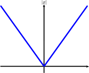
(a) $|x|$

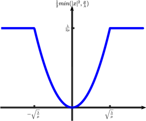
(b) $\frac{1}{2}\min(|x|^{2},\frac{\lambda}{\mu})$

Figure 1: Absolute value function and truncated quadratic function in $\mathbb{R}$.

where $\lambda$ and $\mu$ are positive constants, $X:=\mathbb{R}^{m\times n}$ is a finite dimensional discrete image space, $\nabla=[\nabla_{1},\nabla_{2}]^{T}$ and $f(\boldsymbol{x}):=\|A\boldsymbol{x}-\boldsymbol{x}_{0}\|_{2}^{2}/2$ with $A:X\rightarrow Y_{0}=\mathbb{R}^{m_{0}\times n_{0}}$ being a linear and bounded operator and $\boldsymbol{x}_{0}$ being the noisy or degraded image. Here and subsequently, the $|\cdot|$ norm denotes the usual Euclid norm which is also the length of the corresponding vector. For example, $|(\nabla\boldsymbol{x})_{i,j}|=\sqrt{(\nabla_{1}\boldsymbol{x})_{i,j}^{2}+(\nabla_{2}\boldsymbol{x})_{i,j}^{2}}$ for the isotropic case in (ITQ) and $|(\nabla_{l}\boldsymbol{x})_{i,j}|$ is the absolute value of $(\nabla_{l}\boldsymbol{x})_{i,j}$ with $l=1$ or $l=2$ in (ATQ). $P^{I}$ or $P^{A}$ is the isotropic or anisotropic truncated quadratic regularizations (abbreviated as ITQ or ATQ). The truncated quadratic (also called as half-quadratic) regularization has various applications in signal, image processing and computer vision AIG ; AA ; BVZ ; BZ ; GY ; SC . It was originated from the maximal posterior estimates for the Markov random fields within the probabilistic setting mainly the Bayesian framework GG . It also appeared as the weak membrane energy and the corresponding graduated non-convexity algorithm developed in BZ . The nonsmooth and nonconvex truncated quadratic regularization without gradient operator was also found in robust statistic where it can kill the outliers completely HRRS ; GW ; see Figure 1 for the absolute value function and the truncated quadratic function. The discrete truncated quadratic regularization can also be seen as the discrete version of the continuous variational Mumford-Shah functional CH ; MS1 ; MS2 ; GW . We refer to WLW for the general framework of truncated regularization which covered the truncated quadratic problem. Due to so many important applications in imaging and other fields, there are already a lot of studies on algorithmic developments for this problems NN ; GY . Generally, there are two categories of algorithms. One is the stochastic approximation approach including the simulated annealing and the other is the deterministic approach. There are many kinds of deterministic optimization algorithms including the graph-cut algorithm BVZ and the graduated non-convexity algorithm (GNC) BZ ; see MN ; CLMS for its recent development. Fast algorithms are also developed in AA ; AIG ; CBAB1 ; CBAB2 which benefit from the alternating minimization technique by introducing some auxiliary variables GY ; MD .

Inspired by the recent developments of the difference of convex algorithms (DCA) HAD ; HAD1 ; HAD2 ; YU and the powerful Kurdyka-Łojasiewicz (KL) analysis for nonconvex optimizations AB ; ABRC ; ABS ; LP ; WCP together with the preconditioned techniques in convex splitting algorithms BS1 ; BS2 ; BS3 , we tackle this problem by the proposed preconditioned DCA algorithm with extrapolation. DCA is now widely used for analyzing and computing noncovex models in image and signal processing. For example, a weighted difference of anisotropc and isotropic TV model is proposed in LZOX for better reconstruction and a more delicate $l_{1}$-$\alpha l_{2}$ model is further developed in LCGN . For (ITQ) or (ATQ), we will employ the following difference of convex functions (DC) throughout this paper, $P^{l}(\boldsymbol{x})=P_{1}^{l}(\boldsymbol{x})-P_{2}^{l}(\boldsymbol{x})$ with $l=I$ or $l=A$ and

$$P_{1}^{I}(\boldsymbol{x})=\sum_{i=1}^{m}\sum_{j=1}^{n}\frac{\mu}{2}(|(\nabla\boldsymbol{x})_{i,j}|^{2}+\frac{\lambda}{\mu}),\ P_{2}^{I}(\boldsymbol{x})=\sum_{i=1}^{m}\sum_{j=1}^{n}\frac{\mu}{2}\max{(|(\nabla\boldsymbol{x})_{i,j}|^{2},\frac{\lambda}{\mu})},$$ (1.1)

$$P_{1}^{A}(\boldsymbol{x})=\sum_{i=1}^{m}\sum_{j=1}^{n}\frac{\mu}{2}\sum_{l=1}^{2}(|(\nabla_{l}\boldsymbol{x})_{i,j}|^{2}+\frac{\lambda}{\mu}),\ P_{2}^{A}(\boldsymbol{x})=\sum_{i=1}^{m}\sum_{j=1}^{n}\frac{\mu}{2}\sum_{l=1}^{2}\max{(|(\nabla_{l}\boldsymbol{x})_{i,j}|^{2},\frac{\lambda}{\mu})}.$$

Note that both $f(\boldsymbol{x})$, $P_{1}^{I}(\boldsymbol{x})$ and $P_{2}^{I}(\boldsymbol{x})$ (or $P_{1}^{A}(\boldsymbol{x})$ and $P_{2}^{A}(\boldsymbol{x})$) are convex functions. $P_{1}^{I}$ (or $P_{1}^{A}$) is continuous differentiable with locally Lipschitz gradient and $P_{2}^{I}$ (or $P_{2}^{A}$) is proper closed function. Our motivation mainly comes from the challenging problem for solving the linear subproblems appeared in DCA, which is the most expensive step for DCA in a lot of applications HAD . For example, splitting decomposition algorithm with error control is employed in HAD . We proposed a preconditioned framework and cooperated the preconditioned iteration for linear systems into the total nonlinear DCA iterations. In this framework, only one or few preconditioned steps are needed for the linear subproblems without solving it inexactly or exactly. Especially, the global convergence and the local linear convergent rate of DCA can also be obtained. Usually, the computational amount of one time or few times preconditioned iterations is quite less. For example, the computation effort of one Jacobi or one symmetric Gauss-Seidel iteration for large scale linear system is nearly negligible compared to solving the linear sytem even with moderate accuracy, especially for large scale linear system.

Our contributions belong to the following parts. First, we propose a preconditioned DCA for the truncated quadratic regularization with gradient operator including both the isotropic and anisotropic cases. With the classical preconditioning technique, we can deal with the large linear system efficiently for the nonlinear DCA algorithm with any finite time preconditioned iterations. No error control is needed for solving large linear systems while the convergence can be guaranteed. For example, in the proposed preconditioned framework, one can still obtain global convergence of the DCA by employing 10 specially designed symmetric red-black Gauss-Seidel iterations for the linear subproblem during each DCA iteration. Second, with detailed analysis of the Kurdyka-Łojasiewicz exponent of the minimization functional, together with the global convergence of the iterative sequence, we also prove the local linear convergence rate of the proposed preconditioned DCA. Third, our global convergence and local convergence rate analysis is based on the difference of convex structure (1.1) where $P_{1}$ ($P_{1}^{I}$ or $P_{1}^{A}$) has locally Lipschitz gradient and $P_{2}$ ($P_{2}^{I}$ or $P_{2}^{I}$) is closed and convex. This is different from the case in WCP where $P_{1}$ is closed and convex and $P_{2}$ has locally Lipschitz gradient. Fourth, we also explore the feature of the truncated quadratic regularization for image segmentation within the proposed preconditioned DCA framework, which was already studied by a lot of algorithms including the graduated non-convexity algorithm BZ , the graph-cut based discrete optimization method BVZ , and the primal-dual first-order method SC . Besides the image segmentation, it is known that the truncated quadratic regularization can also be used for image denoising. However, there is no systematic comparisons with the total variation regularization. We give some comparisons between the truncated quadratic regularization and the total variation for image denoising with detailed parameters.

The rest of the paper is organized as follows. In section 2, after some preparations and the calculation of the Kurdyka-Łojasiewicz exponent, we give the global convergence and present the local linear convergence rate of the proposed preconditioned and extrapolated DCA. In section 3, we give a systematic numerical study on the image denoising and image segmentation. Finally, we give some discussions on section 4.

2 Preconditioned DCA_e: convergence and preconditioners

2.1 Preliminaries and KL exponent analysis

Let $h:\mathbb{R}^{n}\rightarrow\mathbb{R}\cup\{+\infty\}$ be a proper lower semicontinuous function. Denote $\operatorname{dom}h:=\{x\in\mathbb{R}^{n}:\ h(x)<+\infty\}$. For each $x\in\operatorname{dom}h$, the limiting-subdifferential of $h$ at $x\in\mathbb{R}^{n}$, written $\partial h$, is defined as follows BM ; Roc1 ,

$$\partial h(x):=\left\{\xi\in\mathbb{R}^{n}:\exists x_{n}\rightarrow x,h(x_{n})\rightarrow h(x),\xi_{n}\rightarrow\xi,\lim_{y\rightarrow x}\inf_{y\neq x_{n}}\frac{h(y)-h(x_{n})-\langle\xi_{n},y-x_{n}\rangle}{|y-x_{n}|}\geq 0\right\}.$$

It is known that the above subdifferential $\partial h$ reduces to the classical subdifferential in convex analysis when $h$ is convex. It can be seen that a necessary condition for $x\in\mathbb{R}^{n}$ to be a minimizer of $h$ is $0\in\partial h(x)$ AB . For the global and local convergence analysis, we also need the Kurdyka-Łojasiewicz (KL) property and KL exponent.

Definition 1 (KL property and KL exponent)

A proper closed function $h$ is said to satisfy the KL property at $\bar{x}\in\operatorname{dom}\partial h$ if there exists $a\in(0,+\infty]$, a neighborhood $\mathcal{O}$ of $\bar{x}$, and a continuous concave function $\psi:[0,a)\rightarrow(0,+\infty)$ with $\psi(0)=0$ such that:

• $\psi$ is continuous differentiable on $(0,a)$ with $\psi^{\prime}>0$.

• For any $x\in\mathcal{O}$ with $h(\bar{x})<h(x)<h(\bar{x})+a$, one has

  $$\psi^{\prime}(h(x)-h(\bar{x}))\operatorname{dist}(0,\partial h(x))\geq 1.$$ (2.1)

A proper closed function $h$ satisfying the KL property at all points in $\operatorname{dom}\partial h$ is called a KL function. If $\psi$ in (2.1) can be chosen as $\psi(s)=cs^{1-\theta}$ for some $\theta\in[0,1)$ and $c>0$, we say that $h$ satisfies KL properties at $\bar{x}$ with exponent $\theta$. This means that for some $\bar{c}>0$, we have

$$\operatorname{dist}(0,\partial h(x))\geq\bar{c}(h(x)-h(\bar{x}))^{\theta}.$$ (2.2)

If $h$ satisfies KL property with exponent $\theta\in[0,1)$ at all the points of $\operatorname{dom}\partial h$, we call $h$ is a KL function with exponent $\theta$.

The following uniformized KL property proved in BST is also important for our discussions.

Lemma 1

Assume $h$ is a proper closed function and $\Gamma$ is a compact set. If $h$ is a constant on $\Gamma$ and satisfies the KL property at each point of $\Gamma$, then there exist $\epsilon,a>0$ for any $\psi$ as in definition 1,

$$\psi^{\prime}(h(x)-h(\hat{x}))\operatorname{dist}(0,\partial h(x))\geq 1,$$ (2.3)

for any $\hat{x}\in\Gamma$ and any $x$ satisfying $\operatorname{dist}(x,\Gamma)<\epsilon$ and $h(\hat{x})<h(x)<h(x)+a$.

The minimization problem (ITQ) or (ATQ) is a standard DC programming and can be solved by DCA. From now on, we will denote $x$ as the vectorized $\boldsymbol{x}$. We will still use the same notations $A$, $\Delta$, $A^{*}$ and $\nabla$ (or $F$, $f$ and $P$) as the matrix version of the linear mappings (the functions) after vectorization. Let’s take the problem (ITQ) for example. The standard DCA iteration reads as follows,

$$x^{t+1}:=\operatorname*{arg\,min}_{x}f(x)+P_{1}^{I}(x)-\langle\xi^{t},x\rangle,\quad\xi^{t}\in\partial P_{2}^{I}(x)|_{x=x^{t}},$$ (2.4)

where $P_{1}^{I}$, $f$ and $P_{1}^{I}$ are the same functions in (1.1) and the term $\langle\xi^{t},x\rangle$ essentially represents the linearization of the convex function $P_{1}^{I}(x)$ through its subgradient. It can be seen by replacing $\langle\xi^{t},x\rangle$ by $\langle\xi^{t},x-x^{t}\rangle+P_{2}^{I}(x^{t})$ in (2.4) without changing the minimization problem (2.4). By direct calculation, the minimizer $x^{k+1}$ of (2.4) can be obtained by solving the following linear equation during each DCA iteration

$$(A^{*}A-\mu\Delta)x=\xi^{t}+A^{*}x_{0}.$$ (2.5)

It is very expensive and challenging to solve this kind of equation especially for large linear systems during each iteration even with error control. In HAD , “preconditioned decomposition algorithm” is employed to solve the equation with error control while $A$ is the identity operator in (2.5). Inspired by the preconditioned framework for the convex splitting algorithm BS1 ; BS2 ; BS3 , our motivation is to introduce the powerful and classical preconditioning technique for linear systems such as (2.5) and cooperate them into the nonlinear DCA.

We introduce the preconditioned iterations for (2.5) through proximal terms with special metric (or weight). Let’s first introduce the inner product and norm induced by the positive definite and self-adjoint operator (metric) $M$,

$$\langle x,y\rangle_{M}:=\langle x,My\rangle,\quad\|x\|_{M}^{2}:=\langle x,Mx\rangle.$$

Moreover, we will also employ the extrapolation framework that can bring out certain acceleration WCP for a lot of cases. The extrapolation strategy is originated from Nesterov’s accelerated gradient method. To this end, let’s introduce the extrapolation parameter $\beta$ such that $\{\beta_{t}\}\subseteq[0,1)$ and $\sup_{t}\beta_{t}<1$. The extrapolation step is done by $y^{t}=x^{t}+\beta_{t}(x^{t}-x^{t-1})$ where the previous iteration $x^{t-1}$ is incorporated. With these preparations, we now give our algorithmic framework, i.e., the Algorithm 1. Henceforth, we will consider the proposed Algorithm 1 with efficient preconditioners for solving the problem.

Algorithm 1 Preconditioned difference-of-convex algorithm with extrapolation (preDCA_e) for $\operatorname*{arg\,min}_{x}F(x)=f(x)+P_{1}(x)-P_{2}(x)$

$x^{0}\in\operatorname{dom}P_{1}$, $\{\beta_{t}\}\subseteq[0,1)$, with $\sup_{t}\beta_{t}<1$. Set $x^{-1}=x^{0}$.

Iterate the following steps for $t=0,1,\cdots$,

$$\xi^{t} \in\partial P_{2}(x^{t}),$$ (2.6)

$$y^{t} =x^{t}+\beta_{t}\left(x^{t}-x^{t-1}\right)$$ (2.7)

$$x^{t+1} =\underset{y}{\arg\min}\left\{\left\langle\nabla f(y^{t})-\xi^{t},y\right\rangle+\frac{1}{2}\|y-y^{t}\|_{M}^{2}+P_{1}(y)\right\}.$$ (2.8)

Unless some stopping criterion is satisfied, stop

Supposing the Lipschitz constant of $f$ in Algorithm 1 is $L$, if choosing $M=L\boldsymbol{I}$ with $\boldsymbol{I}$ denoting the identity operator (or the identity matrix when vectoring $\boldsymbol{x}$), Algorithm 1 reduces to the proximal extrapolation DCA proposed in WCP with different conditions on $P_{1}$ and $P_{2}$. We employ the metric induced by $M$, which can bring out great flexibility to deal with the linear system with efficient preconditioners. Let’s take the following Lemma 2 for example to illustrate our motivation, where we can reformulate (2.8) as the classical preconditioned iteration SA .

Lemma 2

With appropriately chosen linear operator $M\geq L_{0}\boldsymbol{I}$ with positive constant $L_{0}\geq L$, the iteration (2.8) actually can be reformulated as the following classical preconditioned iteration

$$x^{t+1}:=y^{t}+M_{p}^{-1}[b^{t}-Ty^{t}],$$ (2.9)

where

$$b^{t}=L_{0}y^{t}-\nabla f(y^{t})+\xi^{t},\quad T=L_{0}\boldsymbol{I}-\mu\Delta,\quad M_{p}=M-\mu\Delta\geq T.$$

Proof

Denote $b_{1}^{t}=\xi^{t}-\nabla f(y^{t})$. By the structure of $P_{1}^{A}$ or $P_{1}^{I}$ in (1.1), we see

$$M(y-y^{t})-\mu\Delta y-b_{1}^{t}=0.$$

We thus have

$$x^{t+1} =(M-\mu\Delta)^{-1}(b_{1}^{t}+My^{t})$$

$$=(M-\mu\Delta)^{-1}((M-\mu\Delta)y^{t}+b_{1}^{t}+\mu\Delta y^{t})$$

$$=y^{t}+(M-\mu\Delta)^{-1}[b_{1}^{t}+L_{0}y^{t}-(L_{0}\boldsymbol{I}-\mu\Delta)y^{t}],$$

$$=y^{t}+(M-\mu\Delta)^{-1}[b^{t}-(L_{0}\boldsymbol{I}-\mu\Delta)y^{t}],$$ (2.10)

which leads to (2.9) with notation $M_{p}:=M-\mu\Delta$. $M_{p}$ is actually a preconditioner for $T$ to solve the following linear equation

$$Tx=b^{t}.$$ (2.11)

∎

The following remark will give more interpretation of the preconditioned iteration (2.9).

Remark 1

Suppose the discretization of the operator $T=L_{0}\boldsymbol{I}-\mu\Delta$ in Lemma 2 is $D-E-E^{*}$ (still denoting it as $T$ and using $\Delta$ as the discretized $\Delta$) where $D$ is the diagonal part, $-E$ represents the strict lower triangular part and $E^{*}$ is the transpose of $E$. If choosing $M_{p}$ as the symmetric Gauss-Seidel preconditioner for $T$, it is well-known that SA (chapter 4.1) (or BS1 )

$$M_{p}=T+E^{*}D^{-1}E.$$

By Lemma 2, since $M_{p}=(M-\mu\Delta)$, we thus have the explicit form of $M$

$$M=M_{p}+\mu\Delta=T+E^{*}D^{-1}E+\mu\Delta=T+E^{*}D^{-1}E+L_{0}\boldsymbol{I}-(L_{0}\boldsymbol{I}-\mu\Delta)=E^{*}D^{-1}E+L_{0}\boldsymbol{I}.$$

We also see $M\geq L_{0}\boldsymbol{I}$ as in Lemma 2. However, we do not need to calculate the explicit form of $M$ or $M_{p}^{-1}$, since the update (2.9) is exactly the one time symmetric Gauss-Seidel iteration for the linear equation $Ty=b^{t}$ SA . This means that $x^{t+1}$ as in (2.9) is also equivalent to (2.8) through one time symmetric Gauss-Seidel iteration.

For image denosing problem, with $f(x)={\|x-x_{0}\|_{2}^{2}}/{2}$ with Lipschitz constant $1$, if we choose $L_{0}=\boldsymbol{I}$ in Lemma 2, the linear equation (2.11) coincides with the original linear equation of DCA (2.5). For image deblurring problem, one possible choice is that we can still use algorithm 1 with $f(x)={\|Ax-x_{0}\|_{2}^{2}}/{2}$, where the symmetric Gauss-Seidel preconditoners can still be employed for the corresponding perturbed Laplacian equation with using $\nabla f(y^{t})$ explicitly in (2.8). Here, we provide another choice. Taking the (ATQ) for example, letting

$$f=0,\quad P_{1}(y)={\|Ay-x_{0}\|_{2}^{2}}/{2}+P_{1}^{A}(y),\quad P_{2}(y)=P_{2}^{A}(y),$$ (2.12)

we have the following proposition, whose proof is completely similar to Lemma 2 and is thus omitted.

Proposition 1

With appropriately chosen linear operator $M\geq L_{0}\boldsymbol{I}$ with positive constant $L_{0}\geq L$ and the data in (2.12), the iteration (2.8) in Algorithm 1 can be reformulated as the following classical preconditioned iteration

$$x^{t+1}:=y^{t}+M_{p}^{-1}[b^{t}-Ty^{t}],$$ (2.13)

where

$$b^{t}=L_{0}y^{t}+A^{*}x_{0}+\xi^{t},\quad T=L_{0}\boldsymbol{I}+A^{*}A-\mu\Delta,\quad M_{p}=M+A^{*}A-\mu\Delta\geq T.$$

The condition $M\geq L_{0}\boldsymbol{I}$ comes from the positive definite requirement of $M$, which is important for the following convergence analysis. However, we can choose very small $L_{0}$ for the deblurring problem and $T$ can thus approximate the original linear system (2.5). Throughout this paper, if $f=0$ in (2.12) with Lipschitz constant $L=0$, we further assume $M\geq L_{0}\boldsymbol{I}$ with constant $L_{0}>0$.

With Lemma 2, Remark 1, and Proposition 1, it can be seen that one can cooperate the classical preconditioned iteration into the DCA framework through the proximal mapping with metric. We thus can deal with linear systems with powerful tools from the classical preconditioning techniques for linear algebraic equations. Now let’s turn to the KL analysis for the convergence with our preconditioning framework. We begin with the KL exponent of the quadratic functions with an elementary proof.

Lemma 3

The quadratic function ${q}(x)=\frac{1}{2}x^{T}Qx-u^{T}x+s$ is a KL function with KL exponent of $\frac{1}{2}$, where Q is a symmetric positive semidefinite matrix. Moreover, supposing that the minimal positive eigenvalue of $M$ is $\lambda_{M}$, then there exist small positive $\varepsilon$ and $\eta$, such that for any $x$ satisfying $|x-\bar{x}|\leq\varepsilon$ and ${q}(\bar{x})<{q}(x)<{q}(\bar{x})+\eta$, we have

$${q}(x)-{q}(\bar{x})=|{q}(x)-{q}(\bar{x})|\leq\frac{1}{2\lambda_{M}}|\nabla{q}(x)|^{2}.$$

Proof

First, noting that $\frac{1}{2}x^{T}Qx-u^{T}x+s$ and $\frac{1}{2}x^{T}Qx-u^{T}x$ have the same KL exponent, we just need to prove the case of the function ${q}(x)=\frac{1}{2}x^{T}Qx-u^{T}x$ without loss of generality. We first consider the case $\bar{x}$ such that $\nabla{q}(x)|_{x=\bar{x}}=0$, i.e., $Q\bar{x}=u$. Supposing $\lambda_{1}\geq\lambda_{2}\geq\cdots\geq\lambda_{n}\geq 0$ are the eigenvalues of $Q$, we know $\lambda_{M}=\min\{\lambda_{i},\lambda_{i}>0\}$ by assumption. There exists an orthogonal matrix $P$ such that $Q=P^{-1}\text{Diag}[\lambda_{1},\cdots,\lambda_{n}]P$. Furthermore,

$$|{q}(x)-{q}(\bar{x})|=|\frac{1}{2}\langle Q(x-\bar{x}),x-\bar{x}\rangle|$$

$$=\frac{1}{2}(x-\bar{x})^{T}P^{-1}\begin{pmatrix}\lambda_{1}\\ &\ddots\\ &&\lambda_{n}\end{pmatrix}P(x-\bar{x})\leq\frac{1}{2\lambda_{M}}(x-\bar{x})^{T}P^{-1}\begin{pmatrix}\lambda^{2}_{1}\\ &\ddots\\ &&\lambda_{n}^{2}\end{pmatrix}P(x-\bar{x})$$

$$=\frac{1}{2\lambda_{M}}\langle Q(x-\bar{x}),Q(x-\bar{x})\rangle=\frac{1}{2\lambda_{M}}\langle Qx-u,Qx-u\rangle=\frac{1}{2\lambda_{M}}|\nabla{q}(x)|^{2}.$$

Now, let’s turn to the case $|\nabla{q}(\bar{x})|=|Q\bar{x}-u|=\delta_{0}>0$. Supposing $|x-\bar{x}|\leq\varepsilon$, we see

$$|{q}(x)-{q}(\bar{x})| =|\frac{1}{2}x^{T}Qx-u^{T}x-\frac{1}{2}\bar{x}^{T}Q\bar{x}+u^{T}\bar{x}|$$ (2.14)

$$=|\langle\frac{1}{2}(x-\bar{x})^{T}Q(x-\bar{x})+\langle Q\bar{x}-u,x-\bar{x}\rangle|$$

$$\leq\frac{1}{2}\|Q\|\varepsilon^{2}+\delta_{0}\varepsilon.$$

For $|\nabla{q}(x)|^{2}$, we have

$$|\nabla{q}(x)|^{2}=|Qx-u|^{2}=|Qx-Q\bar{x}+Q\bar{x}-u|^{2}$$ (2.15)

$$=|Qx-Q\bar{x}|^{2}+2\langle Q(x-\bar{x}),Q\bar{x}-u\rangle+|Q\bar{x}-u|^{2}\geq\delta_{0}^{2}-\|Q\|^{2}\varepsilon^{2}-2\delta_{0}\|Q\|\varepsilon.$$

To obtain $|{q}(x)-{q}(\bar{x})|\leq\frac{1}{2\lambda_{M}}|\nabla f(x)|^{2}$, one can choose

$$(\delta_{0}^{2}-\|Q\|^{2}\varepsilon^{2}-2\delta_{0}\|Q\|\varepsilon)\frac{1}{2\lambda_{M}}\geq\frac{\delta_{0}^{2}}{2}\frac{1}{2\lambda_{M}}\geq\frac{1}{2}\|Q\|\varepsilon^{2}+\delta_{0}\varepsilon,$$

which leads to

$$\varepsilon\leq\varDelta_{0}:=\min\left(\frac{\delta_{0}}{\|Q\|},\frac{\delta_{0}}{\|Q\|}(\sqrt{\frac{\|Q\|}{2\lambda_{M}}+1}-1)\right).$$

We thus have $|{q}(x)-{q}(\bar{x})|\leq\frac{1}{2\lambda_{M}}|\nabla{q}(x)|^{2}$ for all $|x-\bar{x}|\leq\varDelta_{0}$. The proof is complete. ∎

Remark 2

Lemma 3 can be seen as a special case of Corollary 5.1 of LP , which originated from LL for the convex quadratic problem.

We now discuss the KL exponent of the truncated quadratic regularization functional (ITQ) and (ATQ). We will employ the recent study on KL analysis of the functions which can be written as minimization of a finite number of KL functions with KL exponent $1/2$; see LP . Let’s turn to the following theorem.

Theorem 2.1

Assuming the linear operators $A:X\rightarrow Y_{0}=\mathbb{R}^{m_{0}\times n_{0}}$, $K_{l}:X\rightarrow Y_{l}=\mathbb{R}^{m_{l}\times n_{l}\times c_{l}}$, $l=1,\cdots,k$ are linear, bounded operators and $\mu_{l}$, $\tau_{l}$ are positive parameters, then the KL exponent of the following general truncated quadratic regularization functional $F(\boldsymbol{x})$ is ${1}/{2}$,

$$F(\boldsymbol{x})=\frac{\|A\boldsymbol{x}-\boldsymbol{x}_{0}\|_{2}^{2}}{2}+\sum_{l=1}^{k}\sum_{i=1}^{m_{l}}\sum_{j=1}^{n_{l}}\frac{\mu_{l}}{2}\min(|(K_{l}\boldsymbol{x})_{i,j}|^{2},\tau_{l}).$$ (2.16)

Proof

Let’s first vectorize $\boldsymbol{x}$ and $\boldsymbol{x}_{0}$ as the column vector ${x}\in\mathbb{R}^{mn}$ and ${x}_{0}\in\mathbb{R}^{m_{0}n_{0}}$ correspondingly. We will still use $A$, $K_{l}$, $l=1,\cdots,k$ as the discrete matrix versions of the corresponding linear operators. The equation (2.16) then becomes

$$F({x})=\frac{\|A{x}-{x}_{0}\|_{2}^{2}}{2}+\sum_{l=1}^{k}\sum_{i=1}^{m_{l}n_{l}}\frac{\mu_{l}}{2}\min(|(K_{l}{x})_{i}|^{2},\tau_{l}),$$ (2.17)

where $(K_{l}{x})_{i}$ denote the $i$-th component of $K_{l}{x}$. Note the fact that

$$\min(a,b)+\min(c,d)=\min(a+c,a+d,b+c,b+d),\quad\forall a,b,c,d\in\mathbb{R}.$$

Similarly, for the summation with $N:=\sum_{l=1}^{k}m_{l}n_{l}$ terms with each term of the form $\min(|(K_{l}{x})_{i}|^{2},\tau_{l})$ as in (2.17), we can rewrite $F(x)$ as follows

$$F({x})=\frac{\|A{x}-{x}_{0}\|_{2}^{2}}{2}+\min_{1\leq i\leq 2^{N}}P_{i}(x).$$ (2.18)

$P_{i}(x)$ comes from summing the selected term $|(K_{l}{x})_{i}|^{2}$ or $\tau_{l}$ from $\min(|(K_{l}{x})_{i}|^{2},\tau_{l})$ for $l=1,\cdots,k$ and $i=1,\cdots,m_{l}n_{l}$. For example, we can choose

$$P_{1}(x)=\sum_{l=1}^{k}\sum_{i=1}^{m_{l}n_{l}}\tau_{l},\quad P_{2}(x)=\sum_{l=1}^{k}\sum_{i=1}^{m_{l}n_{l}}|(K_{l}{x})_{i}|^{2}.$$

All the other $P_{i}(x)$ with $i=3,\cdots,2^{N}$ can be chosen similarly. Furthermore, it can be readily checked that each $P_{i}(x)$, $i=1,\cdots,2^{N}$, is a convex quadratic function. It is straightforward that (2.18) can be written as

$$F({x})=\min_{1\leq i\leq 2^{N}}F_{i}(x),\quad F_{i}(x):=\frac{\|A{x}-{x}_{0}\|_{2}^{2}}{2}+P_{i}(x),\quad i=1,\cdots,2^{N}.$$ (2.19)

Actually, we can reformulate each $F_{i}(x)$ in the form of quadratic function as in Lemma 3. Taking the function $F_{2}(x)$ for example, let

$$\Lambda=[A/\sqrt{2},K_{1,1},\cdots,K_{1,m_{1}n_{1}},\cdots,K_{l,1}\cdots,K_{l,m_{l}n_{l}},\cdots,K_{k,1}\cdots,K_{k,m_{k}n_{k}}]^{T},$$

$$b=[x_{0}/\sqrt{2},0,\cdots,0]^{T}\in\mathbb{R}^{N_{0}},\quad N_{0}:=m_{0}n_{0}+\sum_{l=1}^{k}m_{l}n_{l}c_{l},$$

where $K_{i_{1},i_{2}}x=(K_{i_{1}}x)_{i_{2}}$, $i_{1}=1,\cdots,k$, and $i_{2}=1,\cdots,m_{i_{1}}n_{i_{1}}$. We can thus rewrite $F_{2}(x)$ as follows

$$P_{2}(x)=\|\Lambda x-b\|_{2}^{2},$$

which is clearly a quadratic function. Since each $F_{i}(x)$ is a quadratic function as in Lemma 3, then each $F_{i}(x)$ has KL exponent $1/2$ by Lemma 3. With LP (Theorem 3.1) and noting $F(x)$ is a continuous function, we conclude that $F({x})$ is a KL function with an exponent $1/2$, since it can be written as minimization of $F_{i}(x)$ with KL exponent of $1/2$ in (2.19). ∎

Remark 3

For the isotropic model (ITQ), we can choose $m_{0}=m$, $n_{0}=n$, $K_{1}=[\nabla_{1},\nabla_{2}]$ with $m_{1}=n$, $n_{1}=n$, $c_{1}=2$ and $k=1$ as in (2.16). For the anisotropic model (ATQ), we can choose $m_{0}=m$, $n_{0}=n$, $K_{1}=\nabla_{1}$ and $K_{2}=\nabla_{2}$ with $m_{1}=m_{2}=m$, $n_{1}=n_{2}=n$, $c_{1}=c_{2}=1$ and $k=2$ as in (2.16).

Henceforth, we will make extensive use of the following auxiliary function

$${E(x,y)=f(x)+P(x)+\frac{1}{2}\|x-y\|_{M}^{2}=F(x)+\frac{1}{2}\|x-y\|_{M}^{2}.}$$ (2.20)

Let’s calculate the exponent of KL inequality of the auxiliary function $E(x,y)$ in (2.20) at the stationary point. We do this through the relationship between the original function $F(x)$ and the auxiliary function $E(x,y)$.

Lemma 4

If a proper closed function ${F}(x)$ has the KL property at a stationary point $\bar{x}$ with an exponent of $\frac{1}{2}$, then the auxiliary function $E(x,y)={F}(x)+\frac{1}{2}\|x-y\|_{M}^{2}$ has the KL property at the stationary point $(\bar{x},\bar{x})$ with the exponent of $\frac{1}{2}$.

Proof

Because $\bar{x}$ is a stationary point of $F(x)$, we have $0\in\partial F(\bar{x})$. Supposing $0\in\partial E(\bar{x},\bar{y})=({\partial F(\bar{x})+M(\bar{x}-\bar{y})},{M(\bar{y}-\bar{x})})^{T}$, we have $\bar{x}=\bar{y}$ by $M\geq L_{0}\boldsymbol{I}$. Since $F$ has the KL property at $\bar{x}$ with the exponent $\frac{1}{2}$, there exist $c_{1}$, $\epsilon$ and $\eta>0$ such that

$$(F(x)-F(\bar{x}))\leq c_{1}\operatorname{dist}^{2}(0,\partial F(x)),$$ (2.21)

whenever $x\in\operatorname{dom}\partial F(x)$, $\|x-\bar{x}\|\leq\epsilon$ and $F(\bar{x})<F(x)<F(\bar{x})+\eta$. We thus have

$$|E(x,y)-E(\bar{x},\bar{x})| \leq|F(x)-F(\bar{x})|+\frac{1}{2}\|x-y\|_{M}^{2}$$ (2.22)

$$\leq c_{1}\operatorname{dist}^{2}(0,\partial F(x))+\frac{1}{2}\|x-y\|_{M}^{2}$$

for any $(x,y)$ satisfying $x\in\operatorname{dom}\partial F$, $\|x-\bar{x}\|\leq\epsilon$, $\|y-\bar{x}\|\leq\epsilon$ and $E(\bar{x},\bar{x})<E(x,y)<E(\bar{x},\bar{x})+\eta$. Furthermore, if there exists a positive constant $c_{2}$ such that

$$c_{1}\operatorname{dist}^{2}(0,\partial F(x))+\frac{1}{2}\|x-y\|_{M}^{2} \leq c_{2}\operatorname{dist}^{2}(0,\partial E(x,y))$$ (2.23)

$$=c_{2}\operatorname{dist}^{2}((0,0)^{T},(\partial F(x)+M(x-y),M(y-x))^{T}),$$

we get the lemma. For any $\epsilon>0$, we have

$$\operatorname{dist}^{2}(0,\partial E(x,y)) =2\|M(y-x)\|^{2}+\inf_{\xi\in\partial F(x)}(\|\xi\|^{2}+\langle\xi,x-y\rangle_{M})$$ (2.24)

$$\geq 2\|M(y-x)\|^{2}+\inf_{\xi\in\partial F(x)}\left[\|\xi\|^{2}-(\alpha\|\xi\|^{2}+\frac{1}{\alpha}\|M(x-y)\|^{2})\right]$$

$$=(2-\frac{1}{\alpha})\|M(y-x)\|^{2}+(1-\alpha)\operatorname{dist}^{2}(0,\partial F(x))$$

$$\geq(2-\frac{1}{\alpha})\ushort\lambda_{M}\|y-x\|_{M}^{2}+(1-\alpha)\operatorname{dist}^{2}(0,\partial F(x))$$

where the first inequality follows from the inequality $ab\geq-(\alpha a^{2}+\frac{1}{\alpha}b^{2})$, $\forall\alpha>0$ and $\ushort\lambda_{M}$ is the minimum positive eigenvalue of $M$ as before. Setting $\frac{1}{2}<\alpha<1$, we have $1-\alpha>0$ and $2-\frac{1}{\alpha}>0$. With (2.22) and (2.24), to obtain (2.23), one can fix $c_{2}$ as follows

$$\frac{1}{2}\leq c_{2}(2-\frac{1}{\alpha})\ushort\lambda_{M},\quad c_{1}\leq c_{2}(1-\alpha)\Rightarrow c_{2}\geq\max(\frac{c_{1}}{1-\alpha},\frac{\alpha}{(4\alpha-2)\ushort\lambda_{M}})\geq 0.$$ (2.25)

We thus get

$$|E(x,y)-E(\bar{x},\bar{x})|\leq c_{2}\operatorname{dist}^{2}(0,\partial E(x,y)),$$ (2.26)

and the lemma follows. ∎

2.2 Global convergence and local convergence rate

Recall that $\bar{x}$ is a stationary point of $F$ if $0\in\partial F(\bar{x})$. We will first study a property of the iteration (2.8). We further assume $F$ is level-bounded (see Definition 1.8 Roc1 ), i.e., lev${}_{\leq\alpha}F:=\{x:F(x)\leq\alpha\}$ is bounded (or possibly empty). We employ the similar idea in WCP with different conditions on $P_{1}$ and $P_{2}$ here.

Proposition 2

The right hand-side of (2.8): $g(x):=\left\langle\nabla f(y^{t})-\xi^{t},x\right\rangle+\frac{1}{2}\|x-y^{t}\|_{M}^{2}+P_{1}(x)$ is a strongly convex function. Moreover, $g(x^{t+1})\leq g(x^{t})-\frac{1}{2}\|x^{t+1}-x^{t}\|_{M}$ when $x^{t+1}$ is a stationary point of $g(x)$.

Proof

For any $\xi_{1}\in\partial P_{1}(x)$, by the convexity of $\frac{1}{2}\|x-y^{t}\|_{M}$ and $P_{1}(x)$ on $x$, we have

$$g(y)-g(x) =\left\langle\nabla f(y^{t})-\xi^{t},y-x\right\rangle+\frac{1}{2}\|y-y^{t}\|_{M}^{2}-\frac{1}{2}\|x-y^{t}\|_{M}^{2}+P_{1}(y)-P_{1}(x)$$

$$\geq\left\langle\nabla f(y^{t})-\xi^{t},y-x\right\rangle+\frac{1}{2}\|y-x\|_{M}^{2}+\left\langle x-y^{t},y-x\right\rangle_{M}+\left\langle\xi_{1},y-x\right\rangle$$

$$=\left\langle\nabla f(y^{t})-\xi^{t}+M(x-y^{t})+\xi_{1},y-x\right\rangle+\frac{1}{2}\|y-x\|_{M}^{2}$$ (2.27)

$$\geq\left\langle\nabla f(y^{t})-\xi^{t}+M(x-y^{t})+\xi_{1},y-x\right\rangle+\frac{L}{2}\|y-x\|^{2},\ \ \forall x,y\in\operatorname{dom}g.$$

Since

$$\nabla f(y^{t})-\xi^{t}+M(x-y^{t})+\xi_{1}\in\partial g(x),$$

we see $g(x)$ is a strongly convex function with a modulus that is not less than $L_{0}$. Setting $x=x^{t+1}$ and $y=x^{t}$, by the fact that $0\in\partial g(x)|x=x^{t+1}$, according to (2.8), together with (2.27), we have

$$g(x^{t+1})\leq g(x^{t})-\frac{1}{2}\|x^{t+1}-x^{t}\|_{M}.$$ (2.28)

∎

We will first show that the sequence $\{{x^{t}}\}$ generated by the proposed algorithm 1 converges to a stationary point of $E(x,y)$.

Theorem 2.2

Let ${x^{t}}$ be a sequence generated by $preDCA_{e}$ for solving the minimization problem (ITQ) or (ATQ). Then the following statements hold:

• $\displaystyle{\lim_{t\to\infty}\|x^{t+1}-x^{t}\|_{M}=0}$,

• The limit $\displaystyle{\lim_{k\to\infty}E(x^{t},x^{t-1})=:\zeta}$ exists and $E\equiv\zeta$ on $\Upsilon$. Henceforth, we denote $\Upsilon$ as the set of accumulation points of the sequence $(x^{t},x^{t-1})$.

Proof

We first prove (i). By Proposition 2, we can get

$$\left\langle\nabla f(y^{t})-\xi^{t},x^{t}\right\rangle+\frac{1}{2}\|x^{t+1}-y^{t}\|_{M}^{2}+P_{1}(x^{t+1})\\ \leq\left\langle\nabla f(y^{t})-\xi^{t},x^{t+1}\right\rangle+\frac{1}{2}\|x^{t}-y^{t}\|_{M}^{2}+P_{1}(x^{t})-\frac{1}{2}\|x^{t+1}-x^{t}\|_{M}^{2}.$$ (2.29)

On the other hand, since $\nabla f$ is Lipschitz continuous with a modulus of $L$, we have

$$f(x^{t+1})+P(x^{t+1})\leq f(y^{t})+\langle\nabla f(y^{t}),x^{t+1}-y^{t}\rangle+\frac{L}{2}\|x^{t+1}-y^{t}\|^{2}+P_{1}(x^{t+1})-P_{2}(x^{t+1})$$

$$\leq f(y^{t})+\langle\nabla f(y^{t}),x^{t+1}-y^{t}\rangle+\frac{1}{2}\|x^{t+1}-y^{t}\|_{M}^{2}+P_{1}(x^{t+1})-P_{2}(x^{t+1})$$

$$\leq f(y^{t})+\langle\nabla f(y^{t}),x^{t+1}-y^{t}\rangle+\frac{1}{2}\|x^{t+1}-y^{t}\|_{M}^{2}+P_{1}(x^{t+1})-P_{2}(x^{t})-\langle\xi^{t},x^{t+1}-x^{t}\rangle$$

$$\leq f(y^{t})+\langle\nabla f(y^{t}),x^{t}-y^{t}\rangle+\frac{1}{2}\|x^{t}-y^{t}\|_{M}^{2}+P_{1}(x^{t})-P_{2}(x^{t})-\frac{1}{2}\|x^{t+1}-x^{t}\|_{M}^{2}$$

$$\leq f(x^{t})+P(x^{t})+\frac{1}{2}\|x^{t}-y^{t}\|_{M}^{2}-\frac{1}{2}\|x^{t+1}-x^{t}\|_{M}^{2},$$ (2.30)

where the second inequality follows from $M\geq L_{0}\boldsymbol{I}\geq L\boldsymbol{I}$, the third one comes from the fact that $\xi^{t}\in\partial P_{2}(x^{t})$, the fourth inequality follows from (2.28) and the fifth one by the convexity of $f$. From (2.30), we have

$$f(x^{t+1})+P(x^{t+1})\leq f(x^{t})+P(x^{t})+\frac{1}{2}\beta_{t}^{2}\|x^{t}-x^{t-1}\|_{M}^{2}-\frac{1}{2}\|x^{t+1}-x^{t}\|_{M}^{2}.$$

Then, we can obtain that

$$\frac{1}{2}(1-\beta_{t}^{2})\|x^{t}-x^{t-1}\|_{M}^{2}\leq\left[f(x^{t})+P(x^{t})+\frac{1}{2}\|x^{t}-x^{t-1}\|_{M}^{2}\right]$$

$$-\left[f(x^{t+1})+P(x^{t+1})+\frac{1}{2}\|x^{t+1}-x^{t}\|_{M}^{2}\right]=E(x^{t},x^{t-1})-E(x^{t+1},x^{t}).$$ (2.31)

Since ${\beta_{t}}\in\left[0,1\right)$, we see from (2.31) that ${f(x^{t})+P(x^{t})+\frac{1}{2}\|x^{t}-x^{t-1}\|_{M}^{2}}$ is nonincreasing. We can thus get that

$$f(x^{t})+P(x^{t})\leq f(x^{t})+P(x^{t})+\frac{1}{2}\|x^{t}-x^{t-1}\|_{M}^{2}\leq f(x^{0})+P(x^{0}),\ \ \forall t\geq 0,$$

which shows that ${x^{t}}$ is bounded by the level-boundedness of $F$ (Definition 1.8 of Roc1 and WCP ) and $F(x)\geq 0$. Then summing up both sides of (2.31) from $t=0$ to $\infty$, we obtain

$$\frac{1}{2}\sum_{t=0}^{\infty}(1-\beta_{t}^{2})\|x^{t}-x^{t-1}\|_{M}^{2} \leq f(x^{0})+P(x^{0})-\liminf_{t\to\infty}\left[f(x^{t+1})+P(x^{t+1})+\frac{1}{2}\|x^{t+1}-x^{t}\|_{M}^{2}\right]$$

$$\leq f(x^{0})+P(x^{0})<\infty.$$

Since $\sup_{t}\beta_{t}<1$, we deduce from the above inequation that $\sum_{t=1}^{\infty}\|x^{t}-x^{t-1}\|_{M}^{2}<\infty$ and $\lim_{t\to\infty}\|x^{t+1}-x^{t}\|_{M}^{2}=0$. This proves (i).

Now we prove (ii), it can be seen that the sequence ${E(x^{t},x^{t-1})}$ is nonincreasing form (2.31). Together with the fact that $\Upsilon$ is a nonempty compact set due to ${x^{t}}$ is bounded, we conclude that $\zeta:=\lim_{k\to\infty}E(x^{t},x^{t-1})$ exists. Now, let’s show $E\equiv\zeta$ on $\Upsilon$. Taking any $(\bar{x},\bar{x})\in\Upsilon$, there exists a convergent subsequence $(x^{t_{i}},x^{t_{i}-1})$ such that $\lim_{i\to\infty}(x^{t_{i}},x^{t_{i}-1})=(\bar{x},\bar{x})$. Using the fact that $x^{t_{i}}$ is the minimizer of the subproblem in (2.8), we have

$$P_{1}\left(x^{t_{i}}\right)+\left\langle\nabla f\left(y^{t_{i}-1}\right)-\xi^{t_{i}-1},x^{t_{i}}\right\rangle+\frac{1}{2}\|x^{t_{i}}-y^{t_{i}-1}\|_{M}^{2}$$

$$\leq P_{1}(\bar{x})+\left\langle\nabla f\left(y^{t_{i}-1}\right)-\xi^{t_{i}-1},\bar{x}\right\rangle+\frac{1}{2}\|\bar{x}-y^{t_{i}-1}\|_{M}^{2}.$$

Rearranging terms above, we obtain

$$P_{1}\left(x^{t_{i}}\right)+\left\langle\nabla f\left(y^{t_{i}-1}\right)-\xi^{t_{i}-1},x^{t_{i}}-\bar{x}\right\rangle+\frac{1}{2}\|x^{t_{i}}-y^{t_{i}-1}\|_{M}^{2}\leq P_{1}(\bar{x})+\frac{1}{2}\|\bar{x}-y^{t_{i}-1}\|_{M}^{2}.$$ (2.32)

Furthermore, we observe

$$\|\bar{x}-y^{t_{i}-1}\|_{M} =\|\bar{x}-x^{t_{i}}+x^{t_{i}}-y^{t_{i}-1}\|_{M}\leq\|\bar{x}-x^{t_{i}}\|_{M}+\|x^{t_{i}}-y^{t_{i}-1}\|_{M}$$

$$=\|\bar{x}-x^{t_{i}}\|_{M}+\left\|x^{t_{i}}-x^{t_{i}-1}-\beta_{t_{i}-1}\left(x^{t_{i}-1}-x^{t_{i}-2}\right)\right\|_{M}$$

$$\leq\|\bar{x}-x^{t_{i}}\|_{M}+\|x^{t_{i}}-x^{t_{i}-1}\|_{M}+\|x^{t_{i}-1}-x^{t_{i}-2}\|_{M}.$$

Since $\|x^{t+1}-x^{t}\|_{M}\to 0$ and $\lim_{i\to\infty}x^{t_{i}}=\bar{x}$, we have

$$\|\bar{x}-y^{t_{i}-1}\|_{M}\to 0\ \text{ and }\ \|x^{t_{i}}-y^{t_{i}-1}\|_{M}\to 0.$$

Moreover, with (2.32), we obtain

$$\zeta =\lim_{i\to\infty}f\left(x^{t_{i}}\right)+P\left(x^{t_{i}}\right)$$

$$=\lim_{i\to\infty}f\left(x^{t_{i}}\right)+P\left(x^{t_{i}}\right)+\left\langle\nabla f\left(y^{t_{i}-1}\right)-\xi^{t_{i}-1},x^{t_{i}}-\bar{x}\right\rangle+\frac{1}{2}\left\|x^{t_{i}}-y^{t_{i}-1}\right\|_{M}^{2}$$

$$\leq\limsup_{i\to\infty}f\left(x^{t_{i}}\right)+P_{1}(\bar{x})-P_{2}\left(x^{t_{i}}\right)+\frac{1}{2}\left\|\bar{x}-y^{t_{i}-1}\right\|_{M}^{2}=F(\bar{x}).$$

Since $F$ is lower semicontinuous, we have

$$F(\bar{x})\leq\liminf_{i\to\infty}F\left(x^{t_{i}}\right)=\lim_{i\to\infty}F\left(x^{t_{i}}\right)=\zeta.$$ (2.33)

Consequently, $F(\bar{x})=\liminf_{i\to\infty}F(x^{t_{i}})=\zeta$. Noting that for any $(\bar{x},\bar{x})\in\Upsilon$, we have $E(\bar{x},\bar{x})=F(\bar{x})=\zeta$. We thus conclude $E\equiv\zeta$ on $\Upsilon$ and (ii) follows. ∎

Theorem 2.3

Any accumulation point of ${x^{t}}$ is a stationary point of $F$. Furthermore, we have $\sum^{\infty}_{k=1}\|x^{t}-x^{t-1}\|$$\leq\infty$.

Proof

With the same assumption of Theorem 2.2, let $\bar{x}$ be an accumulation of ${x^{t}}$. By the first-order optimality condition of the subproblem (2.8), we get

$$-M(x^{t+1}-y^{t})\in\nabla P_{1}(x^{t+1})+\nabla f(y^{t})-\xi^{t}.$$

With the fact $y^{t}=x^{t}+\beta_{t}(x^{t}-x^{t-2})$, we obtain that

$$-M[(x^{t+1}-x^{t})-\beta_{t}(x^{t}-x^{t-1})]\in\nabla P_{1}(x^{t+1})+\nabla f(y^{t})-\xi^{t}.$$ (2.34)

Because of the convexity of $P_{2}$ and the the boundeness of ${x^{t}}$, by passing to a subsequence if necessary, then $\lim_{i\to\infty}\xi^{t}$ exists without loss of generality, which belongs to $\partial P_{2}(\bar{x})$ due to the closedness of $\partial P_{2}$ (Theorem 8.6 Roc1 ). Using the fact that $\|x^{t+1}-x^{t}\|_{M}^{2}\to 0$ from Theorem 2.2 (ii) together with the closedness of $\nabla P_{1}$ and $\nabla f$, we get upon passing to the limit in (2.34) that

$$0\in\nabla P_{1}(\bar{x})+\nabla f(\bar{x})-\partial P_{2}(\bar{x}).$$

Then, considering the subdifferential of the function $E(x,y)$ at the point $(x^{t},x^{t-1})$, we have

$$\partial E\left(x^{t},x^{t-1}\right)=\left(\nabla f(x^{t})+\nabla P_{1}(x^{t})+M(x^{t}-x^{t-1})-\partial P_{2}(x^{t}),-M(x^{t}-x^{t-1})\right)^{T}.$$ (2.35)

On the other hand, with (2.34) and the fact $\xi^{t}\in\partial P_{2}(x^{t})$, we have

$$(M(x^{t}-x^{t+1}+(1+\beta_{t})(x^{t}-x^{t-1}))+\nabla f(x^{t})-\nabla f(y^{t})+\nabla P_{1}(x^{t})-\nabla P_{1}(x^{t+1}),$$

$$-M(x^{t}-x^{t-1}))^{T}\in\partial E(x^{t},x^{t-1}).$$

Together with the fact that $\nabla f,\nabla P_{1}$ is Lipschitz continuous on a bounded set and $M\geq L\boldsymbol{I}$, we see that there exists $C_{0}>0$ such that

$$\operatorname{dist}((0,0),\partial E(x^{t},x^{t-1})) \leq C_{0}(\|x^{t}-x^{t-1}\|_{M}+\|x^{t+1}-x^{t}\|_{M})$$ (2.36)

$$\leq C(\|x^{t}-x^{t-1}\|+\|x^{t+1}-x^{t}\|),$$

where the constant $C$ depending on $M$ and $C_{0}$. We rewrite (2.31) as

$$E(x^{t},x^{t-1})-E(x^{t+1},x^{t})\geq D_{0}\|x^{t}-x^{t-1}\|_{M}^{2}\geq D\|x^{t}-x^{t-1}\|^{2}.$$ (2.37)

Then, we first consider the case that there exists a $t>0$ such that $E(x^{t},x^{t-1})=\zeta$. Since ${E(x^{t},x^{t-1})}$ is decreasing with the limit $\zeta$, we thus have $E(\bar{x}^{t},\bar{x}^{t-1})=\zeta$ for any $\bar{t}>t$. Hence, $\sum_{t=0}^{\infty}\|x^{t}-x^{t-1}\|_{M}<\infty$ follows easily. We next consider the case that $E(x^{t},x^{t-1})>\zeta$, $\forall t>0$. Since $E$ is a KL function and $E\equiv\zeta$ on $\Upsilon$, by Lemma 1, there exist an $\epsilon>0$ and a continuous concave function $\psi$ with $a>0$ such that

$$\psi^{\prime}(E(x,y)-\zeta)\text{dist}((0,0),\partial E(x,y))\geq 1,\ \ \forall(x,y)\in U,$$ (2.38)

where $U=\left\{(x,y)\in\mathbb{R}^{n}\times\mathbb{R}^{n}:\operatorname{dist}((x,y),\Upsilon)<\epsilon\right\}\cap$ $\left\{(x,y)\in\mathbb{R}^{n}\times\mathbb{R}^{n}:\zeta<E(x,y)<\zeta+a\right\}$. Moreover, we can get that there exists $T>0$ such that

$$\psi^{\prime}\left(E(x^{t},x^{t-1})-\zeta\right)\cdot\operatorname{dist}\left((0,0),\partial E(x^{t},x^{t-1})\right)\geq 1,\ \ \forall t\geq T.$$ (2.39)

Due to $\lim_{t\to\infty}\text{dist}((x^{t},x^{t-1}),\Upsilon)=0$, there thus exists $T_{1}>0$ such that $\operatorname{dist}((x^{t},x^{t-1}),\Upsilon)<\epsilon$ whenvere $t\geq T_{1}$. From the concavity of $\psi$, we see that

$$\begin{array}[]{l}{\left[\psi\left(E(x^{t},x^{t-1})-\zeta\right)-\psi\left(E(x^{t+1},x^{t})-\zeta\right)\right]\cdot\operatorname{dist}\left((0,0),\partial E(x^{t},x^{t-1})\right)}\\ {\left.\geq\psi^{\prime}\left(E(x^{t},x^{t-1})-\zeta\right)\right)\cdot\operatorname{dist}\left((0,0),\partial E(x^{t},x^{t-1})\right)\cdot\left[E(x^{t},x^{t-1})-E(x^{t+1},x^{t})\right]}\\ {\geq E(x^{t},x^{t-1})-E(x^{t+1},x^{t})}.\end{array}$$

Combining this with (2.36) and (2.37), we can get that for any $t\geq T$,

$$\|x^{t}-x^{t-1}\|^{2}\leq \frac{C}{D}\left[\psi\left(E(x^{t},x^{t-1})-\zeta\right)-\psi\left(E(x^{t+1},x^{t})-\zeta\right)\right]$$

$$\cdot\left(\|x^{t}-x^{t-1}\|+\|x^{t-1}-x^{t-2}\|\right).$$

Moreover, we can see further that (by the inequality $a\leq\sqrt{cd}$ $\Rightarrow$ $a\leq c+\frac{d}{4}$ for $a,b,c\geq 0$)

$$\frac{1}{2}\|x^{t}-x^{t-1}\|\leq \frac{C}{D}\left[\psi\left(E(x^{t},x^{t-1})-\zeta\right)-\psi\left(E(x^{t+1},x^{t})-\zeta\right)\right]$$ (2.40)

$$+\frac{1}{4}\left(\|x^{t-1}-x^{t-2}\|-\|x^{t}-x^{t-1}\|\right).$$

Summing up the above relation from $t=T$ to $\infty$, we have

$$\sum_{t=T}^{\infty}\|x^{t}-x^{t-1}\|\leq\frac{2C}{D}\psi\left(E(x^{T},x^{T-1})-\zeta\right)+\frac{1}{2}\|x^{T-1}-x^{\bar{T}-2}\|<\infty.$$ (2.41)

Thus $\{x^{t}\}$ is a Cauchy sequence and its global convergence follows. ∎

Remark 4

Actually, the proofs in Theorems 2.2 and 2.3 have a lot of differences from the proofs in WCP . These are mainly because of two reasons. The first is the proximal term $\|y-y^{t}\|_{M}^{2}/2$ designed for preconditioning which is different from WCP where $M=L\boldsymbol{I}$. The second is the conditions on the functions $P_{1}$ and $P_{2}$ are different from WCP as mentioned in section 1.

We next consider the convergence rate of the sequence $\{x^{t}\}$ under the condition that the auxiliary function $E$ is a KL function at the stationary point whose $\psi$ takes the form $\psi(s)=cs^{1-\theta}$ for $\theta=\frac{1}{2}$, which can be guaranteed by Theorem 2.1 and Lemma 4. This kind of convergence rate analysis is standard; see AB ; ABRC ; LP ; WCP for more comprehensive analysis. We follow a similar line of arguments for the local convergence analysis based on the KL property.

Theorem 2.4

Let ${x^{t}}$ be a sequence generated by preDCA_e for solving (ITQ) or (ATQ) and suppose that ${x^{t}}$ converges to some $\bar{x}$. Since $E$ is a KL function with $\psi$ in KL inequality taking the form $\psi(s)=cs^{1-\theta}$ for $\theta=\frac{1}{2}$ and $c>0$ at the stationary point, then there exist $c_{1}>0,t_{0}>0$ and $\eta\in(0,1)$ such that $\|x^{t}-\bar{x}\|<c_{1}\eta^{t}$ for $\forall t>t_{0}$.

Proof

If there exists $t_{0}>0$ such that $E(x^{t_{0}},x^{t_{0}-1})=\zeta$, then one can show that ${x^{t}}$ is finitely convergent as before and the local linear convergence holds trivially. Hence, we only consider the case when $E(x^{t},x^{t-1})>\zeta$, $\forall t>0$. Define $\Delta_{t}=E(x^{t},x^{t-1})-\zeta$ and $S_{t}=\sum_{i=t}^{\infty}\|x^{i+1}-x^{i}\|$, where $S_{t}$ is well-define thanks to Theorem 2.2 (ii). Then, using (2.40), we have for any $t>T$ that

$$S_{t} =2\sum_{i=t}^{\infty}\frac{1}{2}\|x^{i+1}-x^{i}\|\leq 2\sum_{i=t}^{\infty}\frac{1}{2}\|x^{i}-x^{i-1}\|$$

$$\leq 2\sum_{i=t}^{\infty}\left[\frac{C}{D}\left[\phi(E(x^{i},x^{i-1})-\zeta)-\phi(E(x^{i+1},x^{i})-\zeta)\right]+\frac{1}{4}(\|x^{i-1}-x^{i-2}\|-\|x^{i}-x^{i-1}\|)\right]$$

$$\leq\frac{2C}{D}\phi(E(x^{t},x^{t-1})-\zeta)+\frac{1}{2}\|x^{t-1}-x^{t-2}\|$$

$$=\frac{2C}{D}\phi(\Delta_{t})+\frac{1}{2}(S_{t-2}-S_{t-1})\leq\frac{2C}{D}\phi(\Delta_{t})+\frac{1}{2}(S_{t-2}-S_{t}),$$

where the last inequality follows from the fact that ${S_{t}}$ is nonincreasing. By (2.39) with $\psi(s)=cs^{\frac{1}{2}}$, for all sufficiently large $t$,

$$\frac{c}{2}\Delta_{t}^{-\frac{1}{2}}\text{dist}((0,0),\partial E(x^{t},x^{t-1}))\geq 1.$$

Rewriting (2.36) by the definition of $S_{t}$, we see that for all sufficiently large $t$,

$$\text{dist}((0,0),\partial E(x^{t},x^{t-1}))\leq C(S_{t-2}-S_{t}).$$

We thus can get

$$(\Delta_{t})^{\frac{1}{2}}\leq\frac{Cc}{2}(S_{t-2}-S_{t}).$$

Combining this with $S_{t}\leq\frac{2C}{D}\phi(\Delta_{t})+\frac{1}{2}(S_{t-2}-S_{t})$, we see that for all sufficiently large $t$,

$$S_{t}\leq C_{1}(S_{t-2}-S_{t})+\frac{1}{2}(S_{t-2}-S_{t})=(C_{1}+\frac{1}{2})(S_{t-2}-S_{t}),$$ (2.42)

where $C_{1}=\frac{c^{2}C^{2}}{D}$. Hence,

$$\|x^{t}-\bar{x}\|\leq\sum_{i=t}^{\infty}\|x^{i+1}-x^{i}\|=S_{t}\leq S_{t_{1}-2}\eta^{t-t_{1}+1},\quad\eta:=\sqrt{\frac{2C_{1}+1}{2C_{1}+3}},$$ (2.43)

which completes the proof. ∎

Remark 5

As $L_{0}$ in Lemma 2 is sufficiently large, the upper bound of the convergence rate $\eta$ in (2.43) would decrease as the condition number of $M$ increases.

Proof

Suppose the minmial and maximal eigenvalues of $M$ are $\ushort{\lambda}_{M}$ and $\bar{\lambda}_{M}$. We can see that the convergence rate is related to $c,C$ and $D$ from (2.43). Firstly, we see that $c$ is not related to $M$ for large $L_{0}$, since $\frac{c_{1}}{1-\alpha}\geq\frac{\alpha}{(4\alpha-2)\ushort\lambda_{M}}$ by (2.25), (2.26) and $M\geq L_{0}\boldsymbol{I}$ when $L_{0}$ is large enough. Note that here $c$ is related to $c_{2}$ in (2.26). Furthermore, we can choose $D=\ushort\lambda_{M}D_{0}$ from (2.37) and $C=\sqrt{\bar{\lambda}_{M}}C_{0}$ from (2.36) and the fact $\bar{\lambda}_{M}\|x\|^{2}\geq\|x\|_{M}^{2}\geq\ushort\lambda_{M}\|x\|^{2}$. Since $C_{0},D_{0}$ is not related to $M$, we see $C_{1}=\frac{c^{2}C^{2}}{D}=\frac{c^{2}C_{0}^{2}}{D_{0}}\frac{\bar{\lambda}_{M}}{\ushort{\lambda}_{M}}$ would increase when the condition number of $M$ increases. Thus the upper bound of the convergence rate $\sqrt{1-\frac{2}{2C_{1}+3}}$ is decreased when the condition number of $M$ increases. ∎

2.3 Preconditioners and Preconditioned DCA_e

Let’s first consider the convex subdifferentials $\partial P_{2}^{I}$ or $\partial P_{2}^{A}$ by the following lemma for more general case.

Lemma 5

The subdifferential of the convex function $p(x):=\max(|Kx|^{2},\tau)/2$ is as follows

$$\left\{K^{*}\chi^{s}_{K,\tau}Kx\ |\ s\in[0,1]\right\}=\partial_{x}(\frac{1}{2}\max(|Kx|^{2},\tau)),$$ (2.44)

where the constant $\tau>0$ and $\chi^{s}_{K,\tau}$ is the generalized Clarke derivatives of $\max(\cdot,1.0)$,

$$\chi^{s}_{K,\tau}=\begin{cases}1,\quad&|Kx|/\sqrt{\tau}>1.0,\\ s,\quad&|Kx|/\sqrt{\tau}=1.0,\ s\in[0,1],\\ 0,\quad&|Kx|/\sqrt{\tau}<1.0.\end{cases}$$ (2.45)

Furthermore, we have

$$\partial\left(\sum_{i=1}^{l}\frac{\mu_{i}}{2}\max(|K_{i}x|^{2},\tau_{i})\right)=\left\{\sum_{i=1}^{l}\mu_{i}K_{i}^{*}\chi^{s^{i}}_{K_{i},\tau_{i}}K_{i}x:\ \ s^{i}\in[0,1],\ \ i=1,\cdots,l\right\}.$$ (2.46)

Henceforth, we choose $s^{i}\equiv 1$, $i=1,\cdots,l$ throughout this paper.

Proof

We mainly need to consider (2.45). Since for each $p_{i}(x):=\frac{\mu_{i}}{2}\max(|K_{i}x|^{2},\tau_{i})$, $i=1,\cdots,l$, $\operatorname{dom}p_{i}=X$ which is the whole domain, then by Roc (Theorem 23.8), we have

$$\partial(\sum_{i=1}^{l}p_{i}(x))=\sum_{i=1}^{l}\partial p_{i}(x).$$

Let’s consider the Clarke’s generalized subdifferential of $p(x)$. Denote $p_{1}(x)=\frac{1}{2}|Kx|^{2}$ and $p_{2}(x)=0$. It can be seen that $p(x)$ is a $PC^{1}$ function Sch . It can be easily checked that while $|Kx|>\sqrt{\tau}$,

$$\langle\nabla_{x}(\frac{1}{2}|Kx|^{2}),y\rangle=\langle Kx,Ky\rangle,$$

where the inner product above is understood in the usual vector inner product such as $a^{T}b$. We thus have $(\nabla_{x}p_{1})(y)=\chi^{s}_{K,\tau}\langle Kx,Ky\rangle$ with $s=1$ for $|Kx|>\sqrt{\tau}$. $\nabla_{x}p_{2}(x)=0$ follows easily. We thus conclude that Sch (Proposition 4.3.1)

$$\partial_{x}p(x)=\text{co}\{\nabla_{x}p_{1}(x),\nabla_{x}p_{2}(x)\},$$

where the notation “co” denotes the convex hull of the corresponding set CL . Since for convex functions, the Clarke generalized subdifferential concides with their convex subdifferential CL (Proposition 2.2.7), we have (2.44). ∎

Now we turn to the preconditioners for image denoising. According to Lemma 2, we call a preconditioner $M_{p}$ feasible for $T$ if and only if

$$M_{p}\geq T=L_{0}\boldsymbol{I}-\mu\Delta,$$

where $L_{0}$ is the same as in Lemma 2. For operators of type $T=\alpha\boldsymbol{I}-\beta\Delta$ for $\alpha,\beta>0$ where $\Delta=\operatorname{div}\nabla$ can be interpreted as a discrete Laplace operator with homogeneous Neumann boundary conditions BS1 ; BS2 . In other words: solving $Tx=b$ correspond to a discrete version of the boundary value problem

$$\begin{cases}\alpha\boldsymbol{x}-\beta\Delta\boldsymbol{x}=b,\\ \frac{\partial\boldsymbol{x}}{\partial\nu}|_{\partial\Omega}=0.\end{cases}$$ (2.47)

Besides Remark 1, here are some examples from the classical iterative methods for linear systems.

Example 1

• Obviously, $M_{p}=T$ with $L_{0}=L$ is a feasible preconditioner for $T$ in (2.51). This choice reproduces the original proximal DCA with $M=L\boldsymbol{I}$ without preconditioners.

• The choice $M_{p}=c\boldsymbol{I}$ with $c\geq L+\mu\|\nabla\|^{2}$ also yields a feasible preconditioner. This is corresponding to the Richardson method, where the update for $x^{k+1}$ can be seen as an explicit step.

We employ the efficient symmetric Red-Black Gauss-Seidel (SRBGS) iterations as the preconditioner BS1 ; BS2 . Of course, several steps of this preconditioner can also be performed; see the following Proposition 3. Furthermore, we denote the $n$-fold application of the symmetric Red-Black to the initial guess $x$ and right-hand side $b$ by BS1 ; BS2

$$\operatorname{SRBGS}_{\alpha,\beta}^{n}(x,b)=(\boldsymbol{I}+M_{p}^{-1}(\mathbf{1}_{b}-T))^{n}x$$ (2.48)

making it again explicit that $M_{p}$ and $T$ depend on $\alpha$ and $\beta$.

Proposition 3 (BS1 )

Let $M_{p}$ be a feasible preconditioner for $T$ and $n\geq 1$. Then, applying the preconditioner $n$ times, i.e.,

$$\left\{\begin{aligned} x^{k+(i+1)/n}&=x^{k+i/n}+M_{p}^{-1}(b^{k}-Tx^{k+i/n})\\ i&=0,\ldots,n-1\end{aligned}\right.$$

corresponds to $x^{k+1}=x^{k}+M_{p,n}^{-1}(b^{k}-Tx^{k})$ where $M_{p,n}$ is a feasible preconditioner.

It is proved in BS1 that $M_{p,n}\geq T$. We thus conclude that the corresponding metric in the proximal term in (2.8) $M_{n}$ is positive definite, since $M_{n}=M_{p,n}+\mu\Delta\geq T+\mu\Delta\geq L_{0}\boldsymbol{I}$. Proposition 3 provides great flexibility for choosing how many inner preconditioned iterations for the linear subproblems.

Remembering $\nabla x=[\nabla_{1}x,\nabla_{2}x]^{T}$ and $|\nabla x|^{2}=|\nabla_{1}x|^{2}+|\nabla_{2}x|^{2}$, let’s denote

$$\chi_{x}=\begin{cases}1,\quad|\nabla x|\geq\sqrt{\frac{\lambda}{\mu}},\\ 0,\quad|\nabla x|<\sqrt{\frac{\lambda}{\mu}},\end{cases}\ \chi_{x,1}=\begin{cases}1,\quad|\nabla_{1}x|\geq\sqrt{\frac{\lambda}{\mu}},\\ 0,\quad|\nabla_{1}x|<\sqrt{\frac{\lambda}{\mu}},\end{cases}\ \chi_{x,2}=\begin{cases}1,\quad|\nabla_{2}x|\geq\sqrt{\frac{\lambda}{\mu}},\\ 0,\quad|\nabla_{2}x|<\sqrt{\frac{\lambda}{\mu}}.\end{cases}$$

With these preparations, we give the following Algorithm 2.

Algorithm 2 preDCA_e for image denoising or segmentation of the truncated model (ITQ) or (ATQ) with $A=\boldsymbol{I}$

$x^{0}\in\operatorname{dom}P_{1}$, $\{\beta_{t}\}\subseteq[0,1)$, with $\sup_{t}\beta_{t}<1$. Choose $L_{0}\geq L$ and set $x^{-1}=x^{0}$.

Iterate the following steps for $t=0,1,\cdots$,

$$\xi^{t} =\begin{cases}\nabla^{*}\chi_{x^{t}}\nabla x^{t},\quad\text{for the isotropic case,}\\ (\nabla_{1}^{*}\chi_{x^{t},1}\nabla_{1}+\nabla_{2}^{*}\chi_{x^{t},2}\nabla_{2})x^{t},\quad\text{for the anisotropic case,}\end{cases}$$ (2.49)

$$y^{t} =x^{t}+\beta_{t}(x^{t}-x^{t-1}),$$

$$b^{t} =(L_{0}-I)y^{t}+\nabla f|_{y=y^{t}}+\xi^{t},$$ (2.50)

$$x^{t+1} =\operatorname{SRBGS}_{\alpha,\beta}^{n}(y^{t},b^{t}),\quad T:=(L_{0}\boldsymbol{I}-\mu\Delta).$$ (2.51)

Unless some stopping criterion is satisfied, stop

For color images, denoting the color image as $\textbf{x}=(\boldsymbol{x}_{1},\boldsymbol{x}_{2},\boldsymbol{x}_{3})^{T}$, the truncated quadratic regularization models are as follows

$$\operatorname*{arg\,min}_{\bf x}\mathcal{F}({\bf x})=\frac{\|{\bf A}{\bf x}-{\bf x}_{0}\|_{2}^{2}}{2}+\sum_{i=1}^{m}\sum_{j=1}^{n}\frac{\mu}{2}\min(|(\nabla\textbf{x})_{i,j}|^{2},\frac{\lambda}{\mu}),\ \ \text{isotropic case}$$ (2.52)

$$\operatorname*{arg\,min}_{\bf x}\mathcal{F}({\bf x})=\frac{\|{\bf A}{\bf x}-{\bf x}_{0}\|_{2}^{2}}{2}+\sum_{i=1}^{m}\sum_{j=1}^{n}\sum_{k=1}^{3}\frac{\mu}{2}\min(|(\nabla\boldsymbol{x}_{k})_{i,j}|^{2},\frac{\lambda}{\mu}),\ \ i=1,2,3,\ \ \text{anisotropic case}$$

where $|\nabla{\bf x}|^{2}=\sum_{i=1}^{3}|\nabla\boldsymbol{x}_{i}|^{2}$ and $|\nabla\boldsymbol{x}_{i}|^{2}=|\nabla_{1}\boldsymbol{x}_{i}|^{2}+|\nabla_{2}\boldsymbol{x}_{i}|^{2}$, $i=1,2,3$ and $\bf A$ is a linear and bounded operator. It can be seen that the functional of the isotropic case in (2.52) is still within the form of Theorem 2.1. For the anisotropic case, denoting ${\bf K}_{1}=\text{Diag}[\nabla,0,0]$, ${\bf K}_{2}=\text{Diag}[0,\nabla,0]$ and ${\bf K}_{3}=\text{Diag}[0,0,\nabla]$, then the functional

$$\sum_{i=1}^{3}\frac{\mu}{2}\min(|\nabla\boldsymbol{x}_{i}|^{2},\frac{\lambda}{\mu})=\sum_{i=1}^{3}\frac{\mu}{2}\min(|{\bf K_{i}}{\bf x}|^{2},\frac{\lambda}{\mu}),$$

is still of the form in Theorem 2.1 before the summation over all the pixels as in (2.52). The global convergence and local linear convergence rate also follow. The corresponding algorithm is completely similar to Algorithm 2 and we omit here.

3 Numerics

In this section, we will consider the image denoising and image segmentation problem. All experiments are performed in Matlab 2019a on a 64-bit PC with an Inter(R) Core(TM) i5-6300HQ CPU(2.30Hz) and 12 GB of RAM.

3.1 Image Denoising

We will compare with the well-known total variation (TV) regularization

$$\operatorname*{arg\,min}_{\boldsymbol{x}\in X}F(\boldsymbol{x})=\frac{1}{2}\|A\boldsymbol{x}-f\|_{2}^{2}+\alpha\|\nabla\boldsymbol{x}\|_{1},$$ (3.1)

For image denoising, $A=\boldsymbol{I}$. The first-order primal-dual algorithm is employed for the minimization problem (3.1) CP . We will also compare with the appealing truncated regularization framework developed in WLW including the truncated TV (shorten as TR-TV), truncated logarithmic regularization (shorten as TR-LN), the truncated quadratic regularization (shorten as TR-$l_{2}$), and the weighted difference of anisotropic and isotropic total variation mode (Ani-iso-DCA) LZOX . The TR-$l_{2}$ models are the same as (ITQ) and (ATQ). As in WLW , ADMM (Alternating direction method of multipliers) type method is employed to solve the TR-TV, TR-$l_{2}$, and TR-LN. It is already shown TR-TV and TR-LN can give promising PSNR especially for isotropic cases WLW . Here we focus on the anisotropic cases. The extrapolation parameter $\{\beta_{t}\}$ is chosen according to WCP for the proposed preconditioned DCA, where

$$\beta_{t}=(\theta_{t-1}-1)/{\theta_{t}},\quad\theta_{t}=(1+\sqrt{4\theta_{t-1}^{2}+1})/{2},\quad\theta_{-1}=\theta_{0}=1.$$ (3.2)

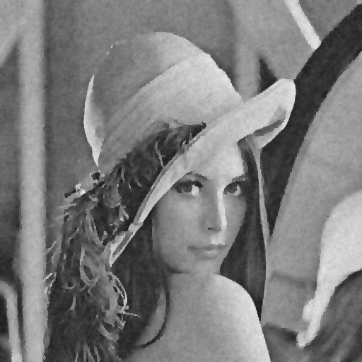
(b) ATQ model with $\lambda=3,\mu=0.01$

(c) TV model, $\alpha=0.1$

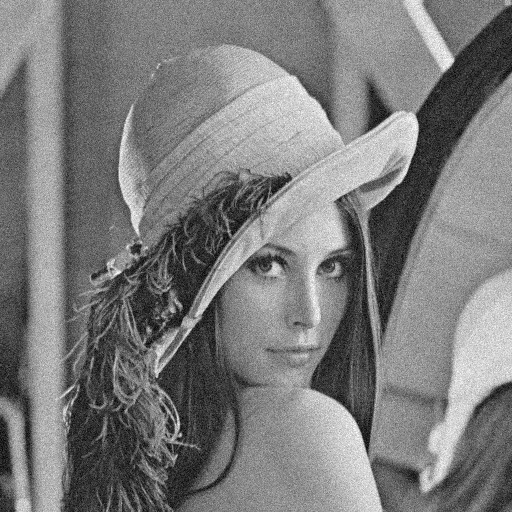
(d) Noisy image with $\sigma=0.05$

(e) ATQ model with $\lambda=1.5,\mu=0.005$

(f) TV model, $\alpha=0.05$

Figure 2: Images (a) and (d) show the corresponding noisy images of the standard Lena image of size $512\times 512$ corrupted by Gaussian noise of Gaussian variance $\sigma=0.1$ and $\sigma=0.05$, i.e., Lena1 and Lena2 image in Table 1. Images (b) and (e) show the denoised images of (a) and (d) with ATQ by parameters $\mu=3,\lambda=0.01$ and $\mu=1.5,\lambda=0.005$ correspondingly. Images (c) and (f) are denoised images of (a) and (d) by the anisotropic TV through the first-order primal-dual algorithm with the corresponding parameters $\alpha=0.1$ and $\alpha=0.05$.

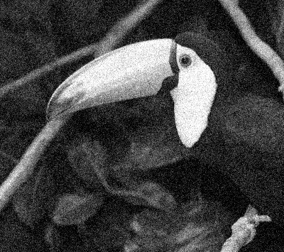
(b) Noisy image with $\sigma=0.1$

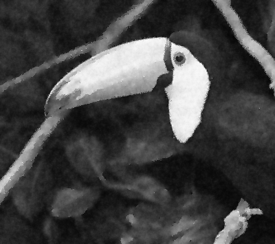
(c) ITQ model with $\lambda=3,\mu=0.01$

Figure 3: Images (a) shows the original $400\times 355$ Tucan image. Image (b) is a noisy image corrupted by 10% Gaussian noise. Image (c) shows the denoised image by (ITQ) with parameters $\mu=3,\lambda=0.01$.

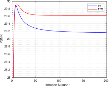
(a) PSNR comparison with iteration number between ATQ and anisotropic TV

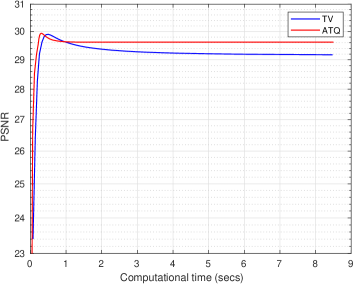
(b) PSNR comparison with iteration time between ATQ and anisotropic TV

Figure 4: Figures (a) or (b) shows the PSNR comparisons with iteration number or computational time between (ATQ) and the anisotropic TV. The computations are based on the Monarch image of size $768\times 512$. The parameters of (ATQ) are $\mu=3,\lambda=0.01$ and the parameter of the anisotropic TV is $\alpha=0.1$.

Restarting strategy is necessary for satisfying the condition $\{\beta_{t}\}\in[0,1)$ and $\sup_{t}\beta_{t}<1$. The adaptive $\beta_{t}$ in (3.2) can bring out certain acceleration experimentally. With appropriate parameters of $\lambda$ and $\beta$, it can be seen that the truncated regularization (ITQ) and (ATQ) can obtain high quality denoised images; see Figure 2 for the anisotropic truncated quadratic case (ATQ) and Figure 3 for the isotropic truncated quadratic case (ITQ). Especially, there is no staircasing effect for (ITQ) or (ATQ) as the total variation. From Figure 4, it can be seen that the (ATQ) can get better PSNR with less iterations and less computation time compared with the anisotropic TV.

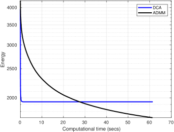
(a) Energy comparison with iteration number between ATQ and anisotropic ADMM

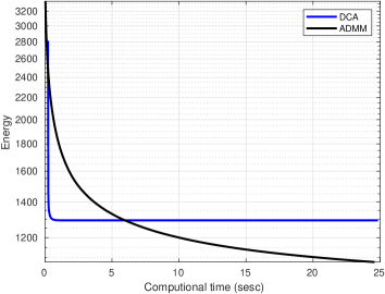
(b) Energy comparison with iteration time between ATQ and anisotropic ADMM

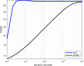
(c) PSNR comparison with iteration number between ATQ and anistropic ADMM

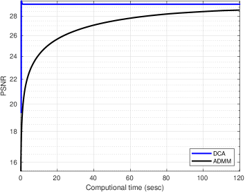
(d) PSNR comparison with iteration time between ATQ and anistropic ADMM

Figure 7: Figures (a) or (b) shows the energy comparisons with iteration number or computational time between (ATQ) and the anisotropic ADMM for image denoising. Figures (c) or (d) shows the PSNR comparison with iteration number or computational time between (ATQ) and the anisotropic ADMM for image denoise. The computations are based on the Lena image of size $512\times 512$ and the zeros mean Gaussian white noise of variance $\sigma=0.1$ are added to the image. The parameters of (ATQ) are $\mu=3,\lambda=0.01$ and the parameters of the anisotropic ADMM is $\alpha=2/3,\beta=6000,\tau=0.0577$.

From Table 1 which is focused on the anisotropic cases, it can be seen that both (ATQ) and TR-LN are very competitive with high PSNR values for most cases compared with TV. The TR-TV can get higher SSIM for some cases. Although the same model with the same parameters $\lambda$ and $\mu$ for (ATQ), our proposed preconditioned DCA can get higher PSNR and SSIM compared with ADMM used in WLW . The preconditioned DCA may exploit more potential of the model (ATQ) compared to the ADMM employed in WLW . For the comparison with computational efficiency, Figure 7 tells that while the proposed preconditioned DCA can decrease the energy quickly and achieve a better PSNR value much fast compared with both iteration number and iteration time, the ADMM employed in WLW can obtain a lower energy with enough iterations. Tables 1 also shows that the Ani-iso-DCA LZOX is also competitive compared to TV. However, it is not as promising as ATQ and TR-LN models.

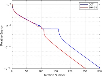
(a) Comparison with iteration number between SRBGS preconditioner and the DCT slover

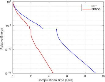
(b) Comparison with iteration time between SRBGS preconditioner and the DCT slover

Figure 5: Figures (a) or (b) shows the comparison with iteration number or computational time between preconditioned DCA with 10 times symmetric Red-Black Gauss-Seidel (SRBGS) iterations and the DCT solver. The DCT solver can be seen as an approximately exact solver without preconditioners, i.e., $M=L\boldsymbol{I}$. The computation is based on Monarch with size $768\times 512$ for the model (ATQ) with parameters $\mu=3,\lambda=0.01$.

For the global convergence with preconditioners, Figure 5 tells that the proposed preconditioned DCA is faster than DCA with solving the linear subproblem very accurately by the DCT (Discrete cosine transform) compared both with iteration number and computational time. This is surprising that the proposed preconditioned DCA not only can save the computational efforts but also can improve the performance of DCA with more efficient algorithms. For the local convergence rate, Figure 6(a) tells that for the whole nonlinear DCA iterations, for the linear system appeared, the SRBGS preconditioner is very efficient compared to solving the linear subproblems very accurately with DCT. The proposed preconditioned DCA can get faster local linear convergence rate with less computations compared to the original proximal DCA with highly accurate DCT solver. Theoretically, the proposed preconditioned DCA not only provides an efficient inexact framework with any finite time preconditioned iterations for DCA with global convergence guarantee, but also can potentially give a faster local convergence rate compared to the original DCA with a very accurate solver.

Figure 8 shows that the proposed preconditioned DCA can be used for image segmentation with various examples, which is not surprising since the truncated quadratic model is widely studied and used for image segmentation problems BVZ ; BZ . Figure 8 also shows that the truncated quadratic model can give better segmentation than TV.

3.2 Image deblurring

For image deblurring, by Proposition 1, we just need to design a preconditioner for the discrete version of the following equation

$$T_{n}\boldsymbol{x}=b^{t},\quad T_{n}:=(L_{0}\boldsymbol{I}+A^{*}A-\mu\Delta_{n}),\quad\frac{\partial\boldsymbol{x}}{\partial\nu}=0,$$ (3.3)

where we use $\Delta_{n}$ to denote the Laplacian operator with emphasis on the Neumann boudary condition. The above equation is usually solved directly by FFT (fast fourier transform). However, considering the FFT is based on the periodic boundary condition which does not match the Neumann boundary condition, it can be circumvented through preconditioning technique BS2 ,

$$T_{p}x=b^{t},\quad T_{p}:=(L_{0}\boldsymbol{I}+A^{*}A-\mu\Delta_{p}),\quad x\ \ \text{with periodic boundary condition},$$ (3.4)

where $\Delta_{p}$ denotes the Laplacian operator with emphasis on the periodic boundary condition. It is proved that $T_{p}\geq T_{n}$ BS2 . We can use $T_{p}$ as a preconditioner for $T_{n}$ as follows

$$x^{t+1}=y^{t}+T_{p}^{-1}(b^{t}-T_{n}y^{t})=T_{p}^{-1}(b^{t}+T_{p}y^{t}-T_{n}y^{t})=T_{p}^{-1}(b^{t}-\mu(\Delta_{p}-\Delta_{n})y^{t}).$$

Since $T_{p}=A^{*}A-\mu\Delta_{n}+M$ by Proposition 1, we have the proximal metric $M=T_{p}-T_{n}+L_{0}\boldsymbol{I}\geq L_{0}\boldsymbol{I}$. Denoting the periodic convolution kernel of $-\Delta$ is $\kappa_{\Delta}$ along with $\mathcal{F}$ and $\mathcal{F}^{-1}$ being the discrete Fourier and inverse Fourier transform BS2 , with these preparations, we now give our Algorithm 3 for image deblurring.

Algorithm 3 preDCA_e for image deblurring of the truncated model (ITQ) or (ATQ) with $Ax=x\ast\kappa$ and $A^{*}x=x\ast\kappa^{\prime}$ with $\kappa$ being the convolution kernel

$x^{0}\in\operatorname{dom}P_{1}$, $\{\beta_{t}\}\subseteq[0,1)$, with $\sup_{t}\beta_{t}<1$. Choose $L_{0}>0$ and set $x^{-1}=x^{0}$.

Iterate the following steps for $t=0,1,\cdots$,

$$\xi^{t} =\begin{cases}\nabla^{*}\chi_{x^{t}}\nabla x^{t},\quad\text{for the isotropic case,}\\ (\nabla_{1}^{*}\chi_{x^{t},1}\nabla_{1}+\nabla_{2}^{*}\chi_{x^{t},2}\nabla_{2})x^{t},\quad\text{for the anisotropic case,}\end{cases}$$ (3.5)

$$y^{t} =x^{t}+\beta_{t}(x^{t}-x^{t-1}),$$

$$b^{t} =L_{0}y^{t}+x_{0}\ast\kappa^{\prime}+\xi^{t},$$ (3.6)

$$x^{t+1} \displaystyle=\mathcal{F}^{-1}\Bigl{(}\frac{\mathcal{F}(b^{t})}{|\mathcal{F}(\kappa)|^{2}+\mu\mathcal{F}(\kappa_{\Delta})+L_{0}}\Bigr{)}.$$ (3.7)

Unless some stopping criterion is satisfied, stop

For image deblurring of anisotropic cases, we will compare with TV, i.e., $Au=u\ast\kappa$ in (3.1) with first-order primal-dual algorithm CP , the TR-TV and TR-$l_{2}$ models in WLW with ADMM who can get stable PSNR during iterations. We also compared with the DCA without preconditioning by $x^{t+1}=T_{p}^{-1}(b^{t})$ and we denote it as ATQ-Npre. In ATQ-Npre, the different boundary conditions of $T_{p}$ and $T_{n}$ are ignored, and FFT together with inverse FFT is directly applied to the Neumann boundary condition $T_{n}$.

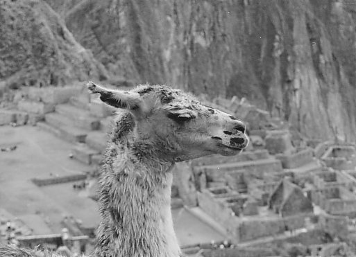
(a) Original image: llama

(b) Degraded image: motion filter, $\sigma=0.01$

(c) ATQ model: $\lambda=0.01$, $\mu=10^{-4}$

(d) Original image: kodim25

(e) Degraded image: Gaussian filter, $\sigma=0.01$

(f) ATQ model: $\lambda=0.01$, $\mu=10^{-4}$

Figure 9: Images (a) or (d) show the original $513\times 371$ Llama image and $720\times 436$ Kodim25 image. Image (b) is degraded Llama2 image by motion blur as in Table 2. Images (c) shows the reconstructed image by (ATQ) with parameters $\mu=0.01,\lambda=10^{-4}$. Image (e) is degraded Kodim251 image with Guassian filter blur as in Table 2. Images (f) shows the reconstructed image by (ATQ) with parameters $\mu=0.01,\lambda=10^{-4}$.

Figure 9 tells that we can get high quality deblurred images with (ATQ) with our preconditioned DCA, i.e., Algorithm 3 for degraded images blurred by motion filter or Gaussian filter. Here we choose $L_{0}=10^{-10}$ to approximate the original linear system (2.5) of the standard DCA. Table 2 shows that (ATQ) with the proposed algorithm can get competitive PSNR and SSIM. Our preconditioned DCA can still obtain better PSNR or SSIM compared the TR-$l_{2}$ by ADMM. Both Table 2 and Figure 6(b) shows that (ATQ) with preconditioned DCA in Algorithm 3 can get better PSNR, SSIM and lower energy compared to the DCA without preconditioning, i.e., ATQ-Npre. The performance of Ani-iso-DCA LZOX is similar to the denoising case, which is competitive compared to TV.

We also found that Algorithm 3 with small $L_{0}$ can get much better PSNR and SSIM than Algorithm 1 for imaging deblurring where the $A^{*}A$ is put into the backward step. Since whose PSNR and SSIM are much lower according to our experience, we did not present the corresponding numerical results.

Table 1: Comparison for anisotropic image denoising models. The noisy images are as follows: Lena1, Lena2 with size $512\times 512$, Monarch1 and Monarch2 with size $768\times 512$. The usual zero mean Gaussian white noise of variance $\sigma=0.1$ for Lena1 or Monarch1 and $\sigma=0.05$ for Lena2 or Monarch2. The parameters for the corresponding models are as follows. For (ATQ), we choose $\mu=3,\lambda=0.01$ for $\sigma=0.1$ cases and $\mu=1.5,\lambda=0.005$ for $\sigma=0.05$ cases. For the anisotropic TV model, the regularization parameter $\alpha$ is chosen as the variance of the noise, i.e., $\alpha=\sigma$. For the truncated regularization, the parameters of TR-TV are $\alpha=10,\beta=600,\tau=0.6$ for $\sigma=0.1$ cases and $\alpha=40,\beta=6000,\tau=0.2$ for $\sigma=.05$ cases. The parameters of TR-$l_{2}$ are $\alpha=2/3,\beta=6000,\tau=0.0577$ for $\sigma=0.1$ cases and $\alpha=4/3,\beta=6000,\tau=0.0577$ for $\sigma=0.05$ cases. The parameters of TR-LN are $\alpha=10,\beta=600,\tau=0.5,\theta=1$ for $\sigma=0.1$ cases and $\alpha=40,\beta=600,\tau=0.5,\theta=1$ for $\sigma=0.05$ cases. The parameters of Ani-iso-DCA are $\mu=5,\lambda=0.5$ for $\sigma=0.1$ cases and $\mu=15,\lambda=1$ for $\sigma=0.05$ cases.

	Lena1		Monarch1		Lena2		Monarch2
	PSNR	SSIM	PSNR	SSIM	PSNR	SSIM	PSNR	SSIM
ATQ model	29.308	0.784	29.620	0.836	32.380	0.859	33.203	0.898
TV model	29.227	0.800	29.143	0.873	31.850	0.854	32.613	0.919
TR-TV	29.250	0.801	29.169	0.875	32.601	0.854	33.178	0.893
TR-$l_{2}$	29.079	0.741	27.851	0.768	31.950	0.832	30.975	0.853
TR-LN	29.285	0.800	29.361	0.873	32.615	0.850	33.223	0.887
Ani-iso-DCA	29.113	0.793	29.227	0.864	32.293	0.859	33.000	0.909

(a) Noisy image with $\sigma=0.1$

(a) Original image: Tucan

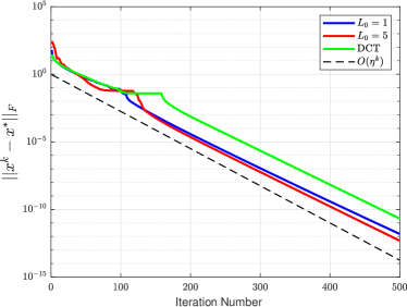
(a) The local linear convergence rate for denoising

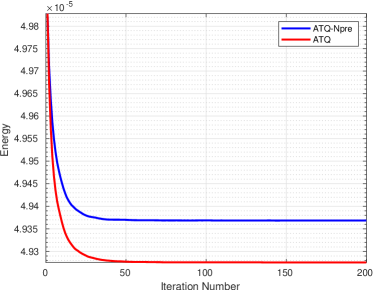
(b) Energy comparison for deblurring

Figure 6: Figure (a): The local linear convergence rate. The computation is by the model (ATQ) for the Monarch image of size $768\times 512$ with parameters $\mu=3,\lambda=0.01$. $L_{0}$ is as in Lemma 2 and DCT represents the case $M=LI$ without preconditoner and solving the corresponding linear equation with DCT solver. The preconditioned DCA for different $L_{0}$ are both with 10 times symmetric Red-Black Gauss-Seidel (SRBGS) iterations. $\eta\in(0,1)$ is a constant. Figure (b): The energy of precondition ATQ is lower that of ATQ without preconditioning (ATQ-Npre) for deblurring the Llama1 image with Motion filter blur and parameters $\mu=0.01,\lambda=10^{-4}$ as in Table 2.

(a) Original Shooter image

(b) ITQ model with $\mu=100,\lambda=0.01$

(c) ATQ model with $\mu=100,\lambda=0.01$

(d) TV model with $\alpha=0.5$

(e) Original Monarch image

(f) ITQ model with $\mu=100,\lambda=0.01$

(g) ATQ model with $\mu=100,\lambda=0.01$

(h) TV model with $\alpha=0.5$

(i) Orignal Flowers color image

(j) ITQ model with $\mu=500,\lambda=0.05$

(k) ATQ model with $\mu=500,\lambda=0.05$

(l) TV model with $\alpha=2$

(m) Original Starfish color image

(n) ITQ model with $\mu=300,\lambda=0.05$

(o) ATQ model with $\mu=300,\lambda=0.05$

(p) TV model with $\alpha=2$

Figure 8: Images (a), (d), (g), (j) show the original gray image Shooter with size $768\times 512$, gray image Monarch with size $768\times 512$, the color image Flowers with size $482\times 321$, the color image Starfish with size $374\times 296$ respectively. The images in the middle column are segmented by (ITQ) while the images in the right column are segmented by (ATQ). Note that the parameters $\mu$ and $\lambda$ can be different for (ITQ) and (ATQ) even for the same image, since we choose the best parameter as we can find.

Table 2: Comparison for anisotropic image deblurring models. The first columns are different degraded images. The Kodim251 and Llama1 are both degraded with Gaussian filter with size $11\times 11$ and Gaussian noise of variance $\sigma=.01$. The Kodim252 and Llama2 are both degraded with motion filter with size $40\times 50$ and Gaussian noise of variance $\sigma=.01$. The corresponding parameters are as follows. We choose $\mu=0.01$ and $\lambda=10^{-4}$ for both ATQ or ATQ-Npre, $\alpha=10^{-3}$ for TV, $\alpha=2000$, $\beta=6000$, $\tau=0.5$ for TR-TV WLW which turns out better than $\beta=600$ as in WLW , $\alpha=400,\beta=500,\tau=0.1$ for TR-$l_{2}$ WLW , $\mu=2,{\lambda=5\times 10^{-3}}$ for Kodim251 and Llama1 cases, and $\mu=5\times 10^{-2}$, $\lambda=5\times 10^{-5}$ for Kodim252 and Llama2 cases. The parameters of Ani-iso-DCA are $\mu=5\times 10^{-2},\lambda=5\times 10^{-5}$ for Gaussian filter and $\mu=2,\lambda=5\times 10^{-3}$ for motion filter. The Kodiam25 image is taken from http://www.cs.albany.edu/~xypan/research/snr/Kodak.html.

	Kodim251		Llama1		Kodim252		Llama2
	PSNR	SSIM	PSNR	SSIM	PSNR	SSIM	PSNR	SSIM
ATQ model	24.211	0.602	27.771	0.750	23.943	0.603	26.820	0.712
TV model	23.655	0.537	26.960	0.704	23.480	0.537	26.081	0.669
TR-TV	23.959	0.571	27.371	0.728	23.936	0.583	26.643	0.700
TR-$l_{2}$	24.112	0.600	27.284	0.707	23.919	0.604	26.450	0.671
ATQ-Npre	24.134	0.599	27.654	0.747	23.835	0.600	26.758	0.710
Ani-iso-DCA	21.832	0.406	24.349	0.562	20.685	0.356	22.962	0.514

4 Discussion and Conclusions

In this paper, we give a thorough study on the proposed preconditioned DCA with extrapolation. We analysis it through the proximal DCA with metric proximal terms. We show that our framework is very efficient to deal with linear systems, while the global convergence and the local convergence rate can also be obtained. Numerical results show that the proposed preconditioned DCA is very efficient for truncated regularization applying to image denoising and image segmentation. We will consider other challenging tasks or applications with our preconditioned DCA framework.

Acknowledgements H. Sun acknowledges the support of NSF of China under grant No.  11701563. The authors also would like to thank all the anonymous referees for their detailed comments that helped us to improve the manuscript.

References

- (1) H. Attouch, J. Bolte, On the convergence of the proximal algorithm for nonsmooth functions involving analytic features, Math. Program., Ser. B, 116, pp. 5–16, 2009, doi:10.1007/s10107-007-0133-5.
- (2) H. Attouch, J. Bolte, P. Redont, A. Soubeyran, Proximal alternating minimization and projection methods for nonconvex problems: an approach based on the Kurdyka-Łojasiewicz inequality, Mathematics of Operations Research, 35(2), pp. 438–457, 2010, doi: 10.1287/moor.1100.0449.
- (3) H. Attouch, J. Bolte, B. F. Svaiter, Convergence of descent methods for semi-algebraic and tame problems: proximal algorithms, forward–backward splitting, and regularized Gauss–Seidel methods, Math. Program., 137, pp. 91–129, 2013, doi:10.1007/s10107-011-0484-9.
- (4) M. Allain, J. Idier, Y. Goussard, On global and local convergence of half-quadratic algorithms, IEEE Trans. Image Process., 15, pp. 1130–1142, 2006.
- (5) G. Aubert, L. Vese, Variational methods in image restoration, SIAM J. Numer. Anal., 34(5), pp. 1948–1979, 1997.
- (6) K. Bredies, H. Sun, Preconditioned Douglas-Rachford splitting methods for convex-concave saddle-point problems, SIAM J. Numer. Anal., 53(1), pp. 421–444, 2015.
- (7) K. Bredies, H. Sun, Preconditioned Douglas–Rachford algorithms for TV- and TGV-regularized variational imaging problems, J. Math. Imaging and Vis., 52(3), pp. 317–344, 2015.
- (8) K. Bredies, H. Sun, A proximal point analysis of the preconditioned alternating direction method of multipliers, Journal of Optimization Theory and Applications, 173(3), pp. 878–907, 2017.
- (9) J. Bolte, S. Sabach, M. Teboulle, Proximal alternating linearized minimization for nonconvex and nonsmooth problems, Math. Program., Ser. A, 146, pp. 459–494, 2014, doi: 10.1007/s10107-013-0701-9.
- (10) Y. Boykov, O. Veksler, R. Zabih, Fast approximate energy minimization via graph cuts, IEEE Trans. Pattern Anal. Mach. Intell., 23, pp. 1222–1239, 2001.
- (11) A. Blake, A. Zisserman, Visual Reconstruction, The MIT Press, 1987.
- (12) A. Chambolle, T. Pock, A first-order primal-dual algorithm for convex problems with applications to imaging, J. Math. Imaging and Vis., 40(1), pp. 120–145, 2011.
- (13) R. Chan, A. Lanza, S. Morigi, F. Sgallari, Convex non-convex image segmentation, Numer. Math., 138, pp. 635–680, 2018.
- (14) A. Chambolle, Image Segmentation by Variational Methods: Mumford and Shah Functional and the Discrete Approximations, SIAM J. Appl. Math., 55(3), pp. 827–863, 1995.
- (15) P. Charbonnier, L. Blanc-Feraud, G. Aubert, M. Barlaud, Two deterministic half-quadratic regularization algorithms for computed imaging, Proceedings of 1st International Conference on Image Processing, Austin, TX, vol.2, pp. 168-172, 1994, doi: 10.1109/ICIP.1994.413553.
- (16) P. Charbonnier, L. Blanc-Feraud, G. Aubert, M. Barlaud, Deterministic edge-preserving regularization in computed imaging, IEEE Trans. Image Process., 6, pp. 298–311, 1997.
- (17) F. H. Clarke, Optimization and Nonsmooth Analysis, Vol. 5, Classics in Applied Mathematics, SIAM, Philadelphia, 1990.
- (18) S. Geman, D. Geman, Stochastic relaxation, Gibbs distributions, and the Bayesian restoration of images, IEEE Trans Pattern Anal Mach Intell., PAMI 6, pp. 721–741, 1984.
- (19) F. R. Hampel, E. M. Ronchetti, P. J. Rousseeuw, W. A. Stahel, Robust Statistics: The Approach Based on Influence Functions, John Wiley & Sons, Inc, 1986.
- (20) D. Geman, C. Yang, Nonlinear image recovery with half-quadratic regularization, IEEE Trans. Image Process., 4(7), pp. 932–946, 1995, doi: 10.1109/83.392335.
- (21) H. A. Le Thi, D. T. Pham, Difference of convex functions algorithms (DCA) for image restoration via a Markov random field model, Optimization and Engineering, 18(4), pp. 873–906, 2017, doi: 10.1007/s11081-017-9359-0.
- (22) H. A. Le Thi, D. T. Pham, Convex analysis approach to D. C. Programming: theory, algorithms and applications, Acta Mthematics Vietnamica, 22(1), pp. 289–355, 1997.
- (23) H. A. Le Thi, D. T. Pham, DC programming and DCA: thirty years of developments, Math. Program., Ser. B, 169, pp. 5-68, 2018, doi: https://doi.org/10.1007/s10107-018-1235-y.
- (24) G. Li, TK Pong, Calculus of the exponent of Kurdyka-Lojasiewicz inequality and its applications to linear convergence of first-order methods, Found. Comput. Math. 18: pp. 1199–1232, 2018, doi: 10.1007/s10208-017-9366-8.
- (25) P. Li, W. Chen, H. Ge, and K. M. Ng, - minimization methods for signal and image reconstruction with impulsive noise removal, Inverse Problems, 36: 055009, 2020.
- (26) Y. Lou, T. Zeng, S. Osher, J. Xin, A weighted difference of anisotropic and isotropic total variation model for image processing, SIAM J. Imag. Sci., 8, pp. 1798-823, 2015.
- (27) X.-D. Luo, Z.-Q. Luo, Extension of Hoffman’s Error Bound to Polynomial Systems, SIAM Journal on Optimization, 4(2), pp. 383–392. 1994, doi:10.1137/0804021.
- (28) B. Mordukhovich, Variational analysis and generalized differentiation I: Basic Theory, Grundlehren der Mathematischen, Wissenschaften, vol. 330, Springer, Heidelberg, 1998.
- (29) D. Mumford, A. Desolneux, Pattern Theory: The Stochastic Analysis of Real-World Signals, A K Peters, Ltd. Natick, Massachusetts, 2010.
- (30) D. Mumford, J. Shah, Boundary detection by minimizing functionals, I, in Proc. IEEE Conf. on Computer Vision and Pattern Recognition, San Francisco, CA, 1985.
- (31) D. Mumford, J. Shah, Optimal approximation by piecewise smooth functions and associated variational problems, Comm. Pure Appl. Math., 42, pp. 577–684, 1989.
- (32) M. Nikolova, Markovian reconstruction using a GNC approach, IEEE Trans. Image Process., 8(9), pp. 1204–1220, 1999.
- (33) M. Nikolova, MK. Ng, Analysis of half-quadratic minimization methods for signal and image recovery, SIAM J. Sci. Comput., 27(3), pp. 937–966, 2005.
- (34) R. T. Rockafellar, Convex Analysis, Princeton University, 1970.
- (35) R. T. Rockafellar, R. Wets, Variational Analysis. Grundlehren der Mathematischen, Wissenschaften, vol. 317, Springer, Heidelberg, 1998.
- (36) Y. Saad, Iterative Methods for Sparse Linear Systems: Second Edition, Society for Industrial and Applied Mathematics, 2003.
- (37) S. Scholtes, Introduction to Piecewise Differentiable Equations, Springer Briefs in Optimization, Springer, New York, 2012.
- (38) E. Strekalovskiy, D. Cremers, Real-time minimization of the piecewise smooth Mumford-Shah functional, In: Fleet D., Pajdla T., Schiele B., Tuytelaars T. (eds) Computer Vision – ECCV 2014, ECCV 2014, Lecture Notes in Computer Science, vol 8690, Springer, Cham.
- (39) B. Wen, X. Chen, TK. Pong, A proximal difference-of-convex algorithm with extrapolation, Comput. Optim. Appl. 69: pp. 297–324, 2018, doi: 10.1007/s10589-017-9954-1.
- (40) G. Winkler, Image Analysis, Random Fields and Markov Chain Monte Carlo Methods : A Mathematical Introduction, Springer-Verlag Berlin Heidelberg, Second Edition, 2003.
- (41) A. L. Yuille, A. Rangarajan, The concave–convex procedure, Neural Comput., 15(4), pp. 915–936, 2003.
- (42) C. Wu, Z. Liu, S. Wen, A general truncated regularization framework for contrast-preserving variational signal and image restoration: Motivation and implementation, Science China Mathematics, 61(9): pp. 1711–1732, 2018.